Approximate Nearest Neighbor Search on High Dimensional Data — Experiments, Analyses, and Improvement (v1.0)

Abstract

Approximate Nearest neighbor search (ANNS) is fundamental and essential operation in applications from many domains, such as databases, machine learning, multimedia, and computer vision. Although many algorithms have been continuously proposed in the literature in the above domains each year, there is no comprehensive evaluation and analysis of their performances.

In this paper, we conduct a comprehensive experimental evaluation of many state-of-the-art methods for approximate nearest neighbor search. Our study (1) is cross-disciplinary (i.e., including 16 algorithms in different domains, and from practitioners) and (2) has evaluated a diverse range of settings, including 20 datasets, several evaluation metrics, and different query workloads. The experimental results are carefully reported and analyzed to understand the performance results. Furthermore, we propose a new method that achieves both high query efficiency and high recall empirically on majority of the datasets under a wide range of settings.

1 INTRODUCTION

Nearest neighbor search finds an object in a reference database which has the smallest distance to a query object. It is a fundamental and essential operation in applications from many domains, including databases, computer vision, multimedia, machine learning and recommendation systems.

Despite much research on this problem, it is commonly believed that it is very costly to find the exact nearest neighbor in high dimensional Euclidean space, due to the curse of dimensionality [26]. Experiments showed that exact methods can rarely outperform the brute-force linear scan method when dimensionality is high [43] (e.g., more than 20). Nevertheless, returning sufficiently nearby objects, referred to as approximate nearest neighbor search (ANNS), can be performed efficiently and are sufficiently useful for many practical problems, thus attracting an enormous number of research efforts. Both exact and approximate NNS problems can also be extended to their top-$k$ versions.

1.1 Motivation

There are hundreds of papers published on algorithms for (approximate) nearest neighbor search, but there has been few systematic and comprehensive comparisons among these algorithms. In this paper, we conduct a comprehensive experimental evaluation on the state-of-the-art approximate nearest neighbor search algorithms in the literature, due to the following needs:

1. Coverage of Competitor Algorithms and Datasets from Different Areas.  As the need for performing ANN search arises naturally in so many diverse domains, researchers have come up with many methods while unaware of alternative methods proposed in another area. In addition, there are practical methods proposed by practitioners and deployed in large-scale projects such as the music recommendation system at spotify.com [7]. As a result, it is not uncommon that important algorithms from different areas are overlooked and not compared with. For example, there is no evaluation among Rank Cover Tree [23] (from Machine Learning), Product Quantization [27, 20] (from Multimedia), SRS [39] (from Databases), and KGraph [15] (from practitioners). Moreover, each domain typically has a small set of commonly used datasets to evaluate ANNS algorithms; there are very few datasets used by all these domains. In contrast, we conduct comprehensive experiments using carefully selected representative or latest algorithms from different domains, and test all of them on 20 datasets including those frequently used in prior studies in different domains. Our study confirms that there are substantial variability of the performances of all the algorithms across these datasets.

2. Overlooked Evaluation Measures/Settings.   An NNS algorithm can be measured from various aspects, including (i) search time complexity, (ii) search quality, (iii) index size, (iv) scalability with respect to the number of objects and the number of dimensions, (v) robustness against datasets, query workloads, and parameter settings, (vi) updatability, and (vii) efforts required in tuning its parameters. Unfortunately, none of the prior studies evaluates these measures completely and thoroughly.

For example, most existing studies use a query workload that is essentially the same as the distribution of the data. Measuring algorithms under different query workloads is an important issue, but little result is known. In this paper, we evaluate the performances of the algorithms under a wide variety of settings and measures, to gain a complete understanding of each algorithm (c.f., Table 6).

3. Discrepancies in Existing Results.   There are discrepancies in the experimental results reported in some of the notable papers on this topic. For example, in the ann-benchmark [8] by practitioners, FLANN was shown to perform better than KGraph, while the study in [15] indicates otherwise. While much of the discrepancies can be explained by the different settings, datasets and tuning methods used, as well as implementation differences, it is always desirable to have a maximally consistent result to reach an up-to-date rule-of-the-thumb recommendation in different scenarios for researchers and practitioners.

In this paper, we try our best to make a fair comparison among all methods evaluated, and test them on all 20 datasets. For example, all search programs are implemented in C++, and all hardware-specific optimizations are disabled (e.g., SIMD-based distance computation). Finally, we will also publish the source codes, datasets, and other documents so that the results can be easily reproduced.

We classify popular $k$NN algorithms into three categories: LSH-based, Space partitioning-based and Neighborhood-based. The key idea of each category of the method will be introduced in Section 3-6.

1.2 Contributions

Our principle contributions are summarized as follows.

• Comprehensive experimental study of state-of-the-art ANNS methods across several different research areas. Our comprehensive experimental study extends beyond past studies by: (i) comparing all the methods without adding any implementation tricks, which makes the comparison more fair; (ii) evaluating all the methods using multiple measures; and (iii) we provide rule-of-the-thumb recommendations about how to select the method under different settings. We believe such a comprehensive experimental evaluation will be beneficial to both the scientific community and practitioners, and similar studies have been performed in other areas (e.g., classification algorithms [12]).

• We group algorithms into several categories (Section 3, 4, 5 and 6), and then perform detailed analysis on both intra- and inter-category evaluations (Sections 8). Our data-based analyses provide confirmation of useful principles to solve the problem, the strength and weakness of some of the best methods, and some initial explanation and understanding of why some datasets are harder than others. The experience and insights we gained throughout the study enable us to engineer a new empirical algorithm, DPG (Section 7), that achieves both high query efficiency and high recall empirically on majority of the datasets under a wide range of settings.

Our paper is organised as follows. Section 2 introduces the problem definition as well as some constraints in this paper. Section 3, 4, 5 and 6 give the descriptions about some state-of-the-art ANNS algorithms that we evaluated. Section 7 presents our improved ANNS approach. The comprehensive experiments and the analyses are reports in Section 8. Section 10 concludes out paper with future work. An evaluation of the parameters of the tested algorithms is reported in Appendix A. Appendix B gives some supplement results of the second round.

2 BACKGROUND

2.1 Problem Definition

In this paper, we focus on the case where data points are $d$-dimensional vectors in $\mathbb{R}^{d}$ and the distance metric is the Euclidean distance. Henceforth, we will use points and vectors interchangeably. Let $\parallel p,q\parallel_{2}$ be the Euclidean distance between two data points $p$ and $q$ and $\mathcal{X}=\{\,x_{1},x_{2},\ldots,x_{n}\,\}$ be a set of reference data points. A $k$NN search for a given query point $q$ is defined as returning $k$ nearest neighbors $kNN(q)\in\mathcal{X}$ with respect to $q$ such that $\left|kNN(q)\right|=k$ and $\forall x\in kNN(q)$, $\forall x^{\prime}\in\mathcal{X}\setminus kNN(q)$, $\parallel x,q\parallel_{2}\leq\parallel x^{\prime},q\parallel_{2}$.

Due to the curse of dimensionality [26], much research efforts focus on the approximate solution for the problem of $k$ nearest neighbor search on high dimensional data. Let the results returned by an algorithm be $X=\{\,x_{i}\mid 1\leq i\leq k\,\}$. A common way to measure the quality of $X$ is its recall, defined as $\frac{\left|X\cap kNN(q)\right|}{k}$, which is also called precision in some papers.

2.2 Scope

The problem of ANNS on high dimensional data has been extensively studied in various literatures such as databases, theory, computer vision, and machine learning. Over hundreds of algorithms have been proposed to solve the problem from different perspectives, and this line of research remains very active in the above domains due to its importance and the huge challenges. To make a comprehensive yet focused comparison of ANNS algorithms, in this paper, we restrict the scope of the study by imposing the following constraints.

Representative and competitive ANNS algorithms.   We consider the state-of-the-art algorithms in several domains, and omit other algorithms that have been dominated by them unless there are strong evidences against the previous findings.

No hardware specific optimizations.   Not all the implementations we obtained or implemented have the same level of sophistication in utilizing the hardware specific features to speed up the query processing. Therefore, we modified several implementations so that no algorithm uses multiple threads, multiple CPUs, SIMD instructions, hardware pre-fetching, or GPUs.

Dense vectors.   We mainly focus on the case where the input data vectors are dense, i.e., non-zero in most of the dimensions.

Support the Euclidian distance.   The Euclidean distance is one of the most widely used measures on high-dimensional datasets. It is also supported by most of the ANNS algorithms.

Exact $k$NN as the ground truth.   In several existing works, each data point has a label (typically in classification or clustering applications) and the labels are regarded as the ground truth when evaluating the recall of approximate NN algorithms. In this paper, we use the exact $k$NN points as the ground truth as this works for all datasets and majority of the applications.

Prior Benchmark Studies

There are two recent NNS benchmark studies:  [34] and ann-benchmark [8]. The former considers a large number of other distance measures in addition to the Euclidean distance, and the latter does not disable general implementation tricks. In both cases, their studies are less comprehensive than ours, e.g., with respect to the number of algorithms and datasets evaluated. More discussions on comparison of benchmarking results are given in Section 9.3.

3 LSH-based methods

These methods are typically based on the idea of locality-sensitive hashing (LSH), which maps a high-dimensional point to a low-dimensional point via a set of appropriately chosen random projection functions. Methods in this category enjoys the sound probabilistic theoretical guarantees on query result quality, efficiency, and index size even in the worst case. On the flip side, it has been observed that the data-independent methods usually are outperformed by data-dependent methods empirically, since the latter cannot exploit the data distribution.

Locality-sensitive hashing (LSH) is first introduced by Indyk and Motwani in [26]. An LSH function family $\mathcal{H}$ for a distance function $f$ is defined as $(r_{1},r_{2},p_{1},p_{2})$-sensitive iff for any two data points $x$ and $y$, there exists two distance thresholds $r_{1}$ and $r_{2}$ and two probability thresholds $p_{1}$ and $p_{2}$ that satisfy: $\small\begin{cases}\Pr_{h\in\mathcal{H}}[h(x)=h(y)]\geq p_{1}&\text{, if }f(x,y)<r_{1}\\ \Pr_{h\in\mathcal{H}}[h(x)=h(y)]\leq p_{2}&\text{, if }f(x,y)>r_{2}\end{cases}$. This means, the chance of mapping two points $x$, $y$ to the same value grows as their distance $f(x,y)$ decreases. The $2$-stable distribution, i.e., the Gaussian/normal distribution, can be used to construct the LSH function family for the Euclidean distance. A data point is mapped to a hash value (e.g., bucket) based on a random projection and discritize method. A certain number of hash functions are used together to ensure the performance guarantee, using different schemes such as the AND-then-OR scheme [14], the OR-then-AND scheme [45], inverted list-based scheme [18, 25], or tree-based scheme [39]. In this category, we evaluate two most recent LSH-based methods with theoretical guarantees: SRS [39] and QALSH [25]. Both of them can work with any $c>1$. Note that we exclude several recent work because either there is no known practical implementation (e.g., [3]) or they do not support the Euclidean distance (e.g., FALCONN [2]). There are also a few empirical LSH-based methods that loses the theoretical guarantees and some of them will be included in other categories.

3.1 SRS

SRS projects the dataset with high dimensionality into a low-dimensional space (no more than 10) to do exact $k$-NN search. We refer the distance between the query $q$ and any point $o$ in original space as $dist(o)$, and the distance in projected space as $\Delta(o)$. The key observation of SRS is for any point $o$, $\frac{\Delta(o)^{2}}{dist(o)^{2}}$ follows the standard $\chi^{2}(m)$ distribution. Hence, The basic method solve a $c$-ANN problem in two steps: (1) obtain an ordered set of candidates by issuing a $k$-NN query with $k=T^{\prime}$ on the $m$-dimensional projections of data points; (2) Examine the distance of these candidates in order and return the points with the smallest distance so far if it satisfies the early-termination test(if there exists a point that is a c-ANN point with probability at least a given threshold) or the algorithm has exhausted the $T^{\prime}$ points. By setting $m=O(1)$, the algorithm guarantees that the returned point is no further away than $c$ times the nearest neighbor distance with constant probability; both the space and time complexities are linear in $n$ and independent of $d$.

3.2 QALSH

Traditionally, LSH functions are constructed in a query-oblivious manner in the sense that buckets are partitioned before any query arrives. However, objects closer to a query may be partitioned into different buckets, which is undesirable. QALSH introduces the concept of query-aware bucket partition and develop novel query-aware LSH functions accordingly. Given a pre-specified bucket width $w$, a hash function $h_{\vec{a},b}(o)=\vec{a}\cdot\vec{o}+b$ is used in previous work, while QALSH uses the function $h_{\vec{a}}(o)=\vec{a}\cdot\vec{o}$ that first projects object $o$ along the random line $\vec{a}$ as before.When a query $q$ arrives, the projection of $q$ (i.e., $h_{\vec{a}}(q)$) is computed and the query projection (or simply the query) is applied as the “anchor” for bucket partition.. This approach of bucket partition is said to be query-aware. In the pre-processing step, the projections of all the data objects along the random line $\vec{a}$ are calculated, and all the data projections are indexed by a $B^{+}$-tree. When a query object $q$ arrives, QALSH computes the query projection and uses the $B^{+}$-tree to locate objects falling in the interval $[h_{\vec{a}}(q)-\frac{w}{2},h_{\vec{a}}(q)+\frac{w}{2}]$. Moverover, QALSH can gradually locate data objects even farther away from the query, just like performing a $B^{+}$-tree range search.

4 Encoding-based Methods

A large body of works have been dedicated to learning hash functions from the data distribution so that the nearest neighbor search result in the hash coding space is as close to the search result in the original space as possible. Please refer to [42, 41] for a comprehensive survey.

Some example methods we evaluated in this category include Neighbor Sensitive Hashing [35], Selective Hashing [19], Anchor Graph Hashing [30], Scalable Graph Hashing [28], Neighborhood APProximation index [34], and Optimal Product Quantization [20].

We exclude a recent work [4] optimizing the performance of product quantization-based method as it is mainly based on utilizing the hardware-specific features.

4.1 Anchor Graph Hashing

The most critical shortcoming of the existing unsupervised hashing methods is the need to specify a global distance measure. On the contrary, in many real-world applications data lives on a low-dimensional manifold, which should be taken into account to capture meaningful nearest neighbors. For these, one can only specify local distance measures, while the global distances are automatically determined by the underlying manifold. AGH is a graph-based hashing method which automatically discovers the neighborhood structure inherent in the data to learn appropriate compact codes in an unsupervised manner.

The first step of the graph-hashing methods is building a neighborhood graph with all the data points. In order to compute the neighborhood graph effectively, AGH builds an approximate neighborhood graph using Anchor Graphs, in which the similarity between a pair of data points is measured with respect to a small number of anchors.The resulting graph is constructed in $O(n)$ time complexity and is sufficiently sparse with performance approaching the true kNN graph as the number of anchors increase.

AGH uses the anchor graph to approximate the neighborhood graph, and accordingly uses the graph Laplacian over the anchor graph to approximate the graph Laplacian of the original graph. Then the eigenvectors can be fastly computed. It also uses a hierarchical hashing to address the boundary issue.

4.2 Scalable Graph hashing

AGH and some representative unsupervised hashing methods directly exploit the similarity (neighborhood structure) to guide the hashing learning procedure, which are considered as a class of graph hashing. Generally, graph hashing methods are expected to achieve better performance than non-graph based hashing methods if the learning algorithms are effective enough. However, graph hashing methods need to compute the pairwise similarities between any two data points. Hence, for large-scale datasets, it is memory-consuming and time-consuming or even intractable to learn from the whole similarity graph. Existing methods have to adopt approximation or sub-sampling methods for graph hashing on large-scale datasets. However, the accuracy of approximation cannot be guaranteed.

SGH adopts a feature transformation method to effectively approximate the whole graph without explicitly computing the similarity graph matrix. Hence, the $O(n^{2})$ computation cost and storage cost are avoided in SGH. The aim of SGH is approximate the similarity matrix $S$ by the learned hashing codes, which resulting in the following objective function:

$$min_{\{b_{l}\}_{l=1}^{n}}\sum_{i,j=1}^{n}(\tilde{S_{ij}}-\frac{1}{c}b_{i}^{T}b_{j})^{2}$$

where $\tilde{S_{ij}}=2S_{ij}-1$. Integrating the idea of kernelized locality-sensitive hashing, the hash function for the $k$-th bit of $b_{i}$ is defined as follow:

$$h_{k}(x_{i})=sgn(\sum_{j=1}^{m}W_{kj}\phi(x_{i},x_{j})+bias_{k})$$

where $W\in R^{c\times m}$ is the weight matrix, $\phi(x_{i},x_{j})$ is a kernel function.

SGH applies a feature transformation method to use all the similarities without explicitly computing $\tilde{S_{ij}}$. The discrete $sgn(.)$ function makes the problem very difficult to solve. SGH uses a sequential learning strategy in a bit-wise manner, where the residual caused by former bits can be complementarily captured in the following bits.

4.3 Neighbor Sensitive Hashing

For hashing-based methods, the accuracy is judged by their effectiveness in preserving the kNN relationships (among the original items) in the Hamming space. That is, the goal of the optimal hash functions is that the relative distance of the original items are ideally linear to relative Hamming distance. To preserve the original distances, existing hashing techniques tend to place the separators uniformly, while those are more effective for rNN searching.

The goal of existing methods is to assign hashcodes such that the Hamming distance between each pair of items is as close to a linear function of their original distance as possible. However, NSH changes the shape of the projection function which impose a larger slope when the original distance between a pair of items is small, and allow the Hamming distance to remain stable beyond a certain distance.

Given a reference point $p$, NSH changes the shape of the projection function which impose a larger slope when the original distance to $p$ is small, and allow the projection distance to remain stable beyond a certain distance. Hence, when using the traditional function under the projection space, it is more likely to be assigned with different hash codes for the points close to $p$. If the distances between the query $q$ and $p$ is smaller than a threshold, the above property also apply to $q$. For handling all possible queries, NSH selects multiple pivots and limits the maximal average distances between a pivot and its closest neighbor pivot to ensure that there will be at least one nearby pivot for any novel query.

4.4 NAPP

permutation methods are dimensionality-reduction approaches, which assess similarity of objects based on their relative distances to some selected reference points, rather than the real distance values directly. An advantage of permutation methods is that they are not relying on metric properties of the original distance and can be successfully applied to non-metric spaces. The underpinning assumption of permutation methods is that most nearest neighbors can be found by retrieving a small fraction of data points whose pivot rankings are similar to the pivot ranking of the query.

A basic version of permutation methods selects $m$ pivots $\Pi_{i}$ randomly from the data points. For each data point $x$, the pivots are arranged in the order of increasing distance from $x$. Such a permutation of pivots is essentially a low-dimensional integer-valued vector whose $i$-th element is the ranking order of the $i$-th pivot in the set of pivots sorted by their distances from $x$. For the pivot closest to the data point, the value of the vector element is one, while for the most distance pivot the value is $m$.

In the searching step, a certain number of candidate points are retrieved whose permutations are sufficiently close to the permutation of the query vector. Afterwards, the search method sorts these candidate data points based on the original distance function.

This basic method can be improved in several ways. For example, one can index permutations rather than searching them sequentially: It is possible to employ a permutation prefix tree, an inverted index, or an index designed for metric spaces, e.g., a VPtree.

Neighborhood APProximation index(NAPP) was implemented by Bilegsaikhan. First, the algorithm selects $m$ pivots and computes the permutations induced by the data points. For each data point, $m_{i}\leq m$ most closest pivots are indexed in a inverted file. At query time, the data points that share at least $t$ nearest neighbor pivots with the query are selected. Then, these candidates points are compared directly against the query based on the real distance.

4.5 Selective Hashing

LSH is designed for finding points within a fixed radius of the query point, i.e., radius search. For a k-NN problem (e.g., the first page results of search engine), the corresponding radii for different query points may vary by orders of magnitude, depending on how densely the region around the query point is populated.

Recently, there has been increasing interest in designing learning-based hashing functions to alleviate the limitations of LSH. If the data distributions only have global density patterns, good choices of hashing functions may be possible. However, it is not possible to construct global hashing functions capturing diverse local patterns. Actually, k-NN distance (i.e., the desired search range) depends on the local density around the query.

Selective Hashing(SH) is especially suitable for k-NN search which works on the top of radius search algorithms such as LSH. The main innovation of SH is to create multiple LSH indices with different granularities (i.e., radii). Then, every data object is only stored in one selected index, with certain granularity that is especially effective for k-NN searches near it.

Traditional LSH-related approaches with multiple indexes include all the data points in every index, while selective hashing builds multiple indices with each object being placed in only one index. Hence, there is almost no extra storage overhead compared with one fixed radius. Data points in dense regions are stored in the index with small granularity, while data points in sparse regions are stored in the index with large granularity. In the querying phase, the algorithm will push down the query and check the cell with suitable granularity.

4.6 Optimal Product Quantization (OPQ)

Vector quantization (VQ) [21] is a popular and successful method for ANN search, which could be used to build inverted index for non-exhaustive search. A vector $x\in\mathbb{R}^{d}$ is mapped to a codeword $\mathbf{c}$ in a codebook $\mathbf{C}=\{\,\mathbf{c}_{j}\,\}$ with $i$ in a finite index set. The mapping, termed as a quantizer, is denoted by: $x\rightarrow\mathbf{c}(i(x))$, where the function $i(\cdot)$ and $\mathbf{c}(\cdot)$ is called encoder and decoder, respectively. The $k$-means approach has been widely used to construct the codebook $\mathbf{C}$ where $i(x)$ is the index of the nearest mean of $x$ and $\mathbf{c}(i(x))$ is corresponding mean. An inverted index can be subsequently built to return all data vectors that are mapped to the same codeword.

A product quantizer [27] is a solution to VQ when a large number of codewords are desired. The key idea is to decompose the original vector space into the Cartesian product of $M$ lower dimensional subspaces and quantize each subspace separately. Suppose $M=2$ and the dimensions are evenly partitioned. Each vector $x$ can be represented as the concatenation of $2$ sub-vectors: $[x^{(1)},x^{(2)}]$, Then we have $\mathbf{C}=\mathbf{C^{(1)}}\times\mathbf{C^{(2)}}$ where $\mathbf{C}^{(1)}$ (resp. $\mathbf{C}^{(2)}$) is constructed by applying the $k$-means algorithm on the subspace consisting of the first (resp. second) half dimensions. As such, there are $k\times k$ codewords, and $x$’s nearest codeword $\mathbf{c}$ in $\mathbf{C}$ is the concatenation of the two nearest sub-codewords $c^{(1)}$ and $c^{(2)}$ based on its sub-vectors $x^{(1)}$ and $x^{(2)}$, respectively. Given a query vector $q=[q^{(1)},q^{(2)}]$, the search algorithm in [6] first retrieves $L$ closest sub-codedwords $\{\,\mathbf{C^{i}_{j}}\,\}_{i\in\{\,1,2\,\},j\in\{\,1,2,\ldots L\,\}}$ in each subspaces based on $q^{(1)}$ and $q^{(2)}$, respectively, and then a multi-sequence algorithm based on a priority queue is applied to traverse the set of pairs $\{\,\mathbf{C^{1}_{j}},\mathbf{C^{2}_{j}}\,\}$ in increasing distance to achieve candidate codeword set $\mathcal{C}$, finally, the distances of points belonging to one of the code word in $\mathcal{C}$ are examined via the inverted index.

Recently, the Optimal Product Quantization (OPQ) method is proposed [20], which optimizes the index by minimizing the quantization distortion with respect to the space decompositions and the quantization codewords.

5 Tree-based Space Partition Methods

Tree-based space partition has been widely used for the problem of exact and approximate NNS. Generally, the space is partitioned in a hierarchically manner and there are two main partitioning schemes: pivoting and compact partitioning schemes. Pivoting methods partition the vector space relying on the distance from the data point to pivots while compact partitioning methods either divide the data points into clusters, approximate Voronoi partitions or random divided space. In this subsection, we introduce two representative compact partitioning methods, Annoy [7] and FLANN [33]. as they are used in a commercial recommendation system and widely used in the Machine Learning and Computer Vision communities. In addition, we also evaluate a classical pivoting partitioning method, Vantage-Point tree [44] (VP-tree), in the experiments.

5.1 FLANN

FLANN is an automatic nearest neighbor algorithm configuration method which select the most suitable algorithm from randomized kd-tree [38], hierarchical k-means tree [17], and linear scan methods for a particular data set. Below, we briefly introduce the two modified tree-based methods and the algorithm selection criteria of FLANN based on [33] and Version 1.8.4 source code.

Randomized kd-trees

The main differences from FLANN’s randomize kd-trees with the traditional kd-tree are: (i) The data points are recursively split into two halves by first choosing a splitting dimension and then use the perpendicular hyperplane centered at the mean of the dimension values of all input data points. (ii) The splitting dimension is chosen at random from top-5 dimensions that have the largest sample variance based on the input data points. (iii) Multiple randomized kd-trees are built as the index.

To answer a query $q$, a depth-first search prioritized by some heuristic scoring function are used to search multiple randomized kd-trees with a shared priority queue and candidate result set. The scoring function always favors the child node that is closer to the query point, and lower bounding distance is maintained across all the randomized trees.

Hierarchical k-means tree  is constructed by partitioning the data points at each level into $K$ regions using K-means clustering. Then the same method is applied recursively to the data points in each region. The recursion is stopped when the number of points in each leaf node is smaller than $K$. The tree is searched by initially traversing the tree from the root to the closest leaf, during which the algorithm always picks up the the inner node closest to the query point, and adding all unexplored branches along the path to a priority queue.

FLANN  carefully chooses one of the three candidate algorithms by minimizing a cost function which is a combination of the search time, index building time and memory overhead to determine the search algorithm. The cost function is defined as follows:

$$c(\theta)=\frac{s(\theta)+\omega_{b}b(\theta)}{min_{\theta\in\Theta}(s(\theta)+\omega_{b}b(\theta))}+\omega_{m}m(\theta)$$

where $s(\theta)$, $b(\theta)$ and $m(\theta)$ represent the search time, tree build time and memory overhead for the trees constructed and queried with parameters $\theta$.

Flann use random sub-sampling cross-validation to generate the data and the query points when we run the optimization. The optimization can be run on the full data set for the most accurate results or using just a fraction of the data set to have a faster auto-tuning process.

5.2 Annoy

Annoy is an empirically engineered algorithm that has been used in the recommendation engine in spotify.com, and has been recognized as one of the best ANN libraries.

Index Construction  .

In earlier versions, Annoy constructs multiple random projection trees [13]. In the latest version (as of March 2016), it instead constructs multiple hierarchical 2-means trees. Each tree is independently constructed by recursively partitioning the data points as follows. At each iteration, two centers are formed by running a simplified clustering algorithm on a subset of samples from the input data points. The two centers defines a partition hyperplane which has equidistant from the centers. Then the data points are partitioned into two sub-trees by the hyperplane, and the algorithm builds the index on each sub-trees recursively.

Search  .

The search process is carried out by traveling tree nodes of the multiple RP trees. Initially, the roots of the RP trees are pushed into a maximum priority queue with key values infinity. For a given tree node $n_{i}$ with parent node $n_{p}$, if the query $q$ falls into the subtree of $n_{i}$, the key of $n_{i}$ is the minimum of its parent node and the distance to the hyperplane; otherwise, the key is the minimum of its parent node and the negative value of the distance to the hyperplane. At each iteration, the node with the maximum key is chosen for exploration.

5.3 VP-tree

VP-tree is a classic space decomposition tree that recursively divides the space with respect to a randomly chosen pivot $\pi$. For each partition, a median value R of the distance from $\pi$ to every other point in the current partition was computed. The pivot-centered ball with the radius $R$ is used to partition the space: the inner points are placed into the left subtree, while the outer points are placed into the right subtree (points that are exactly at distance $R$ from $\pi$ can be placed arbitrarily). Partitioning stops when the number of points falls below the threshold $b$.

In classic VP-tree, the triangle inequality can be used to prune unpromising partitions as follows: imagine that $r$ is a radius of the query and the query point is inside the pivot-centered ball (i.e., in the left subtree). If $R-d(\pi,q)>r$, the right partition cannot have an answer and the right subtree can be safely pruned. The nearest-neighbor search is simulated as a range search with a decreasing radius: Each time we evaluate the distance between $q$ and a data point, we compare this distance with $r$. If the distance is smaller, it becomes a new value of $r$. In [34], a simple polynomial pruner is employed. More specifically, the right partition can be pruned if the query is in the left partition and $(R-d(\pi,q))^{\beta}\alpha_{left}>r$. The left partition can be pruned if the query is in the right partition and $(d(\pi,q)-R)^{\beta}\alpha_{left}>r$.

6 Neighborhood-based Methods

In general, the neighborhood-based methods build the index by retaining the neighborhood information for each individual data point towards other data points or a set of pivot points. Then various greedy heuristics are proposed to navigate the proximity graph for the given query. In this subsection, we introduce the representative neighborhood-based methods, namely Hierarchical Navigable Small World(HNSW [32]) and KGraph [16]. In addition, we also evaluate other two representative methods including Small World (SW [31]), and Rank Cover Tree (RCT [23]) .

6.1 KGraph

KGraph [15] is the representative technique for K-NN graph construction and nearest neighbor searches.

Index Construction  .K-NN graph is a simple directed graph where there are $K$ out-going edges for each node, pointing to its $K$ nearest data points. Since the exact computation of K-NN graph is costly, many heuristics have been proposed in the literature [16, 5]. In [16], the construction of K-NN graph relies on a simple principle: A neighbor’s neighbor is probable also a neighbor. Starting from randomly picked $k$ nodes for each data point, it iteratively improves the approximation by comparing each data point against its current neighbors’ neighbors, including both K-NN and reverse K-NN points, and stop when no improvement can be made. Afterwards, four optimizations are applied (local join, incremental search, sampling and early termination) to reduce the redundant computation and speed up the indexing phrase to stop at an acceptable accuracy.

Search  .A greedy search algorithm is employed in [16] to discover the $k$ nearest neighbor from a query point $q$. Starting from $p$ randomly chosen nodes (i.e.,data points), the search maintains a node list to store the current best $k$ nodes sorted by their distances to the query, and recursively computes the distances from the query $q$ to each neighbor point (by following the graph edges) of first unexplored data point of the node list. The node list is updated by the neighbor points that are closer to the query. This greedy algorithm stops when each data point $x$ at the node list is closer to the query than any of its neighbor.

6.2 Small World

A small world(SW) method is a variant of a navigable small world graph data structure. The small world graph contains an approximation of the Delaunay graph and has long-range links together with the small-world navigation property.SW uses the same searching method with K-NNG. The greatest difference between K-NNG and SW is the connection structure of nodes. K-NNG strives to obtain the local approximate optimal solution for each node, but SW explore the current optimal links for the inserted points by a incremental construction strategy. Besides, SW keeps two-way connection for each edge, but K-NNG only preserve the kNN neighbors of each node.

Index Construction The construction of SW is a bottom-top procedure that insert all the data points consecutively. For every new incoming point,they find the set of its closest neighbors from the graph and the undirected edges are created to connect the set and the point. As more and more elements are inserted into the graph, links that previously served as short-range links now become long-range links making a navigable small world.

Search The nearest neighbor search algorithm is, thus, a greedy search procedure that carries out several sub-searches. A sub-search starts at a random node and proceeds to expanding the set of traversed nodes which are not visited by following neighboring links. The sub-search stops when it cannot find points that are closer than already found $M$ nearest points ($M$ is a search parameter).

6.3 Hierarchical Navigable Small World

The key idea of the Hierarchical Navigable Small World(HNSW) algorithm is to separate the links according to their length scale. In this case, the average connections per element in all of the layers can be limited.

Index Construction HNSW can be seen as a multi-layer and multi-resolution variant of a proximity graph. A ground (zero-level) layer includes all data points and higher layer has fewer points. Similar to SW, HNSW is constructed by incrementially inserting data points, one by one. For each data point, a maximum level $m$ is selected randomly and the new point is added to all the layers starting from layer $m$ down to the layer zero. The insertion process can be divided into two phrases. The first phrase starts from the top layer to $m+1$ by greedily traversing the graph in order to find the closest neighbor in the layer, which is used as the enter point to continue the search in the next layer. The second phrase starts from layer $m$ down to zero. $M$ nearest neighbors are found and connected with the new point. The searching quality is controlled by the parameter $ef$, which is the number of the enter points and plays the similar role with $p$ of KGraph. In first phrase, the number of $ef$ is set as 1.

Search The searching algorithm is roughly equivalent to the insertion algorithm from an item with maximum level $m=0$. The closest neighbors found at the ground layer are returned as the search result.

6.4 Rank Cover Tree

Rank cover tree (RCT)  [23] is a probabilistic data structure for similarity search, which entirely avoids the use of numerical constraints such as triangle inequality. The searching algorithm is based on the ranks of the points with respect to the query, and returns a correct result in time that depends competitively on a measure of the intrinsic dimensionality of the data set.

The structure of RCT blends some of the design features of SASH  [24] and Cover Tree  [9]. It is a hierarchical tree in which each node in the bottom level (level 0) is associated with a data point, and the nodes in level $j$ are randomly selected from the set of level $j-1$ with certain probability. The index construction of RCT is performed by inserting the nodes from high levels to low levels. If one node $x$ in level $j$ appears in the RCT tree, the indexing algorithm will search its nearest neighbor $v$ in level $j+1$, and then link $x$ to $v$. Otherwise, the node links to its copy in level $j+1$.

Searching of RCT starts from the root of the tree, and on each level $j$, only a subset of nodes $V_{j}$ is kept, as the nodes in $V_{j}$ are the most similar to the query. The search algorithm iteratively perform the above procedure until reaching the bottom level.

7 Diversified Proximity Graph

The experience and insights we gained from this study enable us to engineer a new method, Diversified Proximity Graph (DPG), which constructs a different neighborhood graph to achieve better and more robust search performance.

7.1 Motivation

In K-NN graph construction, we only consider the distances of neighbors for each data point. But intuitively we should also consider the coverage of the neighbors. As shown in Figure  1, the two closest neighbors of the point $p$ are $a_{3}$ and $a_{4}$, and hence in the $2$-NN graph $p$ cannot lead the search to the NN of $q$ (i.e., the node $b$) although it is close to $b$. Since $a_{1},\ldots,a_{4}$ are clustered, it is not cost-effective to retain both $a_{3}$ and $a_{4}$ in the K-NN list of $p$. This motivates us to consider the direction diversity (i.e., angular dissimilarity) of the K-NN list of $p$ in addition to the distance, leading to the diversified K-NN graph. Regarding the example, including $a_{3}$ and $b$ is a better choice for the K-NN list of $p$.

[scale = 1.5] [color=black] (4.02,2.3) circle (0pt); [fill=black] (3.92,2.3) circle (1.5pt); [color=black] (3.92,2.3) node (p) ; [color=black] (4.,2.12) node $p$; [fill=black] (3.1,2.82) circle (1.5pt); [fill=black] (3.1,2.82) node (a1) ; [color=black] (3.2,3.0) node $a_{4}$; [fill=black] (2.94,2.36) circle (1.5pt); [fill=black] (2.94,2.36) node (a2) ; [color=black] (2.8,2.25) node $a_{3}$; [fill=black] (2.9,2.8) circle (1.5pt); [color=black] (2.8,2.98) node $a_{1}$; [fill=black] (3.22,1.74) circle (1.5pt); [fill=black] (2.94,2.6) circle (1.5pt); [color=black] (2.8,2.58) node $a_{2}$; [fill=black] (5.2,2.8) circle (1.5pt); [fill=black] (5.2,2.8) node (c) ; [color=black] (5.3,3.0) node $b$;

[color=black] (3.9,3.2) node (s) ;

[color=black] (5.1,2.22)– ++(-1.5pt,-1.5pt) – ++(2.0pt,2.0pt) ++(-2.0pt,0) – ++(2.0pt,-2.0pt); [color=black] (5,2.) node (q) $q$; [-¿,dash pattern=on 3pt off 3pt] (p) – (c); [-¿] (p) – (a1); [-¿,red,snake=zigzag,segment amplitude=3pt,segment length=6pt] (s) – (p); [-¿] (p) – (a2); [fill=black] (2.44,2.84) circle (1.5pt); [fill=black] (1.78,2.44) circle (1.5pt); [fill=black] (2.42,2.36) circle (1.5pt); [fill=black] (2.2,1.92) circle (1.5pt); [fill=black] (5.84,2.44) circle (1.5pt); [fill=black] (5.7,3.) circle (1.5pt); [fill=black] (6.4,2.68) circle (1.5pt); [fill=black] (6.14,2.02) circle (1.5pt);

Figure 1: Toy Example of a $2$-d dataset, $K=2$

Now assume we have replaced edge $(p,a_{4})$ with the edge $(p,b)$ (i.e., the dashed line in Figure 1), but there is still another problem. As we can see that there is no incoming edge for $p$ because it is relatively far from two clusters of points (i.e., $p$ is not $2$-NN of these data points). This implies that $p$ is isolated, and two clusters are disconnected in the example. This is not uncommon in high dimensional data due to the phenomena of “hubness”[36] where a large portion of data points rarely serve as K-NN of other data points, and thus have no or only a few incoming edges in the K-NN graph. This motivates us to also use the reverse edges in the diversified K-NN graph; that is, we keep an bidirected diversified K-NN graph as the index, and we name it Diversified Proximity Graph (DPG).

7.2 Diversified Proximity Graph

The construction of DPG is a diversification of an existing K-NN graph, followed by adding reverse edges.

Given a reference data point $p$, the similarity of two points $x$ and $y$ in $p$’s K-NN list $\mathcal{L}$ is defined as the angle of $\measuredangle xpy$, denoted by $\theta(x,y)$. We aim to choose a subset of $\kappa$ data points, denoted by $\mathcal{S}$, from $\mathcal{L}$ so that the average angle between two points in $\mathcal{S}$ is maximized; or equivalently, $\mathcal{S}=\operatorname*{arg\,min}_{\mathcal{S}\subseteq\mathcal{N},|\mathcal{S}|=\kappa}\sum_{o_{i},o_{j}\in\mathcal{S}}\theta(o_{i},o_{j})$.

The above problem is NP-hard [29]. Hence, we design a simple greedy heuristic. Initially, $\mathcal{S}$ is set to the closest point of $p$ in $\mathcal{L}$. In each of the following $\kappa-1$ iterations, a point is moved from $\mathcal{L}\setminus\mathcal{S}$ to $\mathcal{S}$ so that the average pairwise angular similarity of the points in $\mathcal{S}$ is minimized. Then for each data point $u$ in $\mathcal{S}$, we include both edges $(p,u)$ and $(u,p)$ in the diversified proximity graph. The time complexity of the diversification process is $O(\kappa^{2}Kn)$ where $n$ is the number of data points, and there are totally at most $2\kappa n$ edges in the diversified proximity graph.

It is critical to find a proper $K$ value for a desired $\kappa$ in the diversified proximity graph as we need to find a good trade-off between diversity and proximity. In our empirical study, the DPG algorithm usually achieves the best performance when $K=2\kappa$. Thus, we set $K=2\kappa$ for the diversified proximity graph construction. Although the angular similarity based DPG algorithm can achieve very good search performance, the diversification time of $O(\kappa^{2}Kn)$ is still costly. In our implementation, we use another heuristic to construct the diversified K-NN graph as follows. We keep a counter for each data point in the K-NN list $\mathcal{L}$ of the data point $p$. For each pair of points $u$, $v$ $\in\mathcal{L}$, we increase the counter of $v$ by one if $v$ is closer to $u$ than to $p$; that is, $\parallel v,u\parallel_{2}$ $<\parallel v,p\parallel_{2}$. Then, we simply keep the $\kappa$ data points with lowest count frequencies for $p$ because, intuitively, the count of a data point is high if there are many other points with similar direction. This leads to the time complexity of $O(K^{2}n)$ for diversification. Our empirical study shows that we can achieve similar search performance, while significantly reduce the diversification time. We also demonstrate that both diversification and reverse edges contribute to the improvement of the search performance.

Note that the search process of the DPG is the same as that of KGraph introduced in Section 6.1.

8 EXPERIMENTS

In this section, we present our experimental evaluation.

8.1 Experimental Setting

8.1.1 Algorithms Evaluated

We use $15$ representative existing NNS algorithms from the three categories and our proposed diversified proximity graph (DPG) method. All the source codes are publicly available. Algorithms are implemented in C++ unless otherwise specified. We carefully go through all the implementations and make necessary modifications for fair comparisons. For instance, we re-implement the search process of some algorithms in C++. We also disable the multi-threads, SIMD instructions, fast-math, and hardware pre-fetching technique. All of the modified source codes used in this paper are public available on GitHub [40].

(1) LSH-based Methods.   We evaluate Query-Aware LSH [25] (QALSH, PVLDB’15) and SRS [39] (SRS, PVLDB’14).

(2) Encoding-based Methods.   We evaluate Scalable Graph Hashing [28] (SGH, IJCAI’15), Anchor Graph Hashing [30] (AGH, ICML’11), Neighbor-Sensitive Hashing [35] (NSH, PVLDB’15). We use the hierarchical clustering trees in FLANN to index the resulting binary vectors to support more efficient search for the above algorithms. Due to increased sparsity for the Hamming space with more bits, precision within Hamming radius 2 drops significantly when longer codes are used. Therefore, we check the real distances of at most $N$ data points to achieve the tradeoff between the search quality and search speed.

We also evaluate the Selective Hashing [19] (SH, KDD’15) , Optimal Product Quantization[20] (OPQ, TPAMI’14) and Neighborhood APProximation index [34] (NAPP, PVLDB’15). Note that we use the inverted multi-indexing technique [6] to perform non-exhaustive search for OPQ.

(3) Tree-based Space Partition Methods.   We evaluate FLANN ([33], TPAMI’14), Annoy, and an advanced Vantage-Point tree [10] (VP-tree10, NIPS’13).

(4) Neighborhood-based Methods.   We evaluate Small World Graph [31] (SW10, IS’14), Hierarchical Navigable Small World [32](HNSW10, CoRR’16), Rank Cover Tree [23] (RCT, TPAMI’15), K-NN graph [16, 15] (KGraph, WWW’11), and our diversified proximity graph (DPG14).

Computing Environment.   All C++ source codes are complied by g++ $4.7$, and MATLAB source codes (only for index construction of some algorithms) are compiled by MATLAB $8.4$. All experiments are conducted on a Linux server with Intel Xeon $8$ core CPU at $2.9$GHz, and $32$G memory.

8.1.2 Datasets and Query Workload

We deploy $18$ real datasets used by existing works which cover a wide range of applications including image, audio, video and textual data. We also use two synthetic datasets. Table 1 summarizes the characteristics of the datasets including the number of data points, dimensionality, Relative Contrast (RC [22]), local intrinsic dimensionality (LID [1]), and data type where RC and LID are used to describe the hardness of the datasets.

Relative Contrast evaluates the influence of several crucial data characteristics such as dimensionality, sparsity, and database size simultaneously in arbitrary normed metric spaces.

Suppose $X=\{x_{i},i=1,...,n\}$ and a query $q$ where $x_{i}$, $q\in R^{d}$ are i.i.d samples from an unknown distribution $p(x)$. Let $D_{min}^{q}=\min_{i=1,...,n}{D(x_{i},q)}$ is the distance to the nearest database sample, and $D_{mean}^{q}=E_{x}[D(x,q)]$ is the expected distance of a random database sample from the query $q$. The relative contrast of the dataset X for a query $q$ is defined as $C_{r}^{q}=\frac{D_{mean}^{q}}{D_{min}^{q}}$. The relative contrast for the dataset X is given as $C_{r}=\frac{E_{q}[D_{mean}^{q}]}{E_{q}[D_{min}{q}]}=\frac{D_{mean}}{D_{min}}$.

Intuitively, $C_{r}$ captures the notion of difficulty of NN search in $X$. Smaller the $C_{r}$, more difficult the search. If $C_{r}$ is close to 1, then on average a query $q$ will have almost the same distance to its nearest neighbor as that to a random point in $X$.

We also can define Relative Contrast for $k$-nearest neighbor setting as $C_{r}^{k}=\frac{D_{mean}}{D_{knn}}$, where $D_{knn}$ is the expected distance to the $k$-th nearest neighbor. Smaller RC value implies harder datasets.

Local Intrinsic Dimensionality evaluates the rate at which the number of encountered objects grows as the considered range of distances expands from a reference location. We employ RVE(estimation using regularly varying funtions) to compute the value of LID. It applies an ad hoc estimator for the intrinsic dimensionality based on the characterization of distribution tails as regularly varying functions. The dataset with higher LID value implies harder than others.

We mark the first four datasets in Table 1 with asterisks to indicate that they are “hard” datasets compared with others according to their RC and LID values.

Below, we describe the datasets used in the experiments.

Nusw includes around $2.7$ million web images, each as a $500$-dimensional bag-of-words vector.

Gist is an image dataset which contains about 1 million data points with 960 dimensions.

Random contains $1$M randomly chosen points in a unit hypersphere with dimensionality $100$.

Glove contains 1.2 million 100-d word feature vectors extracted from Tweets.

Cifar is a labeled subset of TinyImage dataset, which consists of 60000 32 $\times$ color images in 10 classes, with each image represented by a 512-d GIST feature vector.

Audio has about 0.05 million 192-d audio feature vectors extracted by Marsyas library from DARPA TIMIT audio speed dataset.

Mnist consists of 70k images of hand-written digits, each as a 784-d vector concatenating all pixels.

Sun397 contains about 0.08 million 512-d GIST features of images.

Enron origins from a collection of emails. yifang et. al. extract bi-grams and form feature vectors of 1369 dimensions.

Trevi consists of 0.4 million $\times$ 1024 bitmap(.bmp) images, each containing a 16 $\times$ 16 array of image patches. Each patch is sampled as 64 $\times$ 64 grayscale, with a canonical scale and orientation. Therefore, Trevi patch dataset consists of around 100,000 4096-d vectors.

Notre contains about 0.3 million 128-d features of a set of Flickr images and a reconstruction.

Youtube_Faces contains 3,425 videos of 1,595 different people. All the videos were downloaded from YouTube. 0.3 million vectors are extracted from the frames , each contains 1770 features.

Msong is a collection of audio features and metadata for a million contemporary popular music tracks with $420$ dimensions.

Sift consists of 1 million 128-d SIFT vectors.

Deep dataset contains deep neural codes of natural images obtained from the activations of a convolutional neural network, which contains about 1 million data points with 256 dimensions.

UKbench contains about 1 million 128-d features of images.

ImageNet is introduced and employed by “The ImageNet Large Scale Visual Recognition Challenge(ILSVRC)”, which contains about 2.4 million data points with 150 dimensions dense SIFT features.

Gauss is generated by randomly choosing $1000$ cluster centers with in space $[0,10]^{512}$, and each cluster follows the a Gaussian distribution with deviation $1$ on each dimension.

UQ_Video is video dataset and the local features based on some keyframes are extracted which include 256 dimensions.

Bann is used to evaluate the scalability of the algorithms, where $1$M, $2$M, $4$M, $6$M, $8$M, and $10$M data points are sampled from $128$-dimensional SIFT descriptors extracted from natural images.

Name	$n$ $(\times 10^{3})$	$d$	RC	LID	Type
Nus*	269	500	1.67	24.5	Image
Gist*	983	960	1.94	18.9	Image
Rand*	1,000	100	3.05	58.7	Synthetic
Glove*	1,192	100	1.82	20.0	Text
Cifa	50	512	1.97	9.0	Image
Audio	53	192	2.97	5.6	Audio
Mnist	69	784	2.38	6.5	Image
Sun	79	512	1.94	9.9	Image
Enron	95	1,369	6.39	11.7	Text
Trevi	100	4,096	2.95	9.2	Image
Notre	333	128	3.22	9.0	Image
Yout	346	1,770	2.29	12.6	Video
Msong	922	420	3.81	9.5	Audio
Sift	994	128	3.50	9.3	Image
Deep	1,000	128	1.96	12.1	Image
Ben	1,098	128	1.96	8.3	Image
Imag	2,340	150	2.54	11.6	Image
Gauss	2,000	512	3.36	19.6	Synthetic
UQ-V	3,038	256	8.39	7.2	Video
BANN	10,000	128	2.60	10.3	Image

Table 1: Dataset Summary

Query Workload. Following the convention, we randomly remove $200$ data points as the query points for each datasets. The average performance of the $k$-NN searches is reported. The $k$ value varies from $1$ to $100$ in the experiments with default value $20$. In this paper, we use Euclidean distance for ANNS.

8.2 Evaluation Metrics

Since exact $k$NN can be found by a brute-force linear scan algorithm (denoted as $\mathit{BF}$), we use its query time as the baseline and define the speedup of Algorithm $A$ as $\frac{t_{\mathit{BF}}}{t_{A}}$, where $t_{x}$ is the average search time of Algorithm $x$.

The search quality of the $k$ returned points is measured by the standard recall against the $k$NN points (See Section 2.1).

All reported measures are averaged over all queries in the query workload. We also evaluate other aspects such as index construction time, index size, and scalability.

Note that the same algorithm can achieve different combination of speedup and recall (typically via using different threshold on the number of points verified, i.e., $N$).

8.3 Parameter Tunning

Below are the default settings of the key parameters of the algorithms in the second round evaluation in Section 8.5.

• SRS. The number of projections ($m$) is set to $8$.

• OPQ. The number of subspaces is $2$, and each subspace can have $2^{10}$ codewords (i.e., cluster centers) by default.

• Annoy. The number of the Annoy trees, $m$, is set to $50$.

• FLANN. We let the algorithm tune its own parameters.

• HNSW. The number of the connections for each point, $M$, is set to $10$.

• KGraph. By default, we use $K=40$ for the K-NN graph index.

• DPG. We use $\kappa=\frac{K}{2}=20$ so that the index size of DPG is the same as that of KGraph in the worst case.

More details about how to tune each algorithm and the comparisons about our counting_based DPG and angular_based DPG were reported in Appendix A.

8.4 Comparison with Each Category

In this subsection, we evaluate the trade-offs between speedup and recall of all the algorithms in each category. Given the large number of algorithms in the space partition-based category, we evaluate them in the encoding-based and tree-based subcategories separately. The goal of this round of evaluation is to select several algorithms from each category as the representatives in the second round evaluation (Section 8.5).

8.4.1 LSH-based Methods

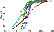
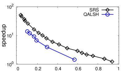
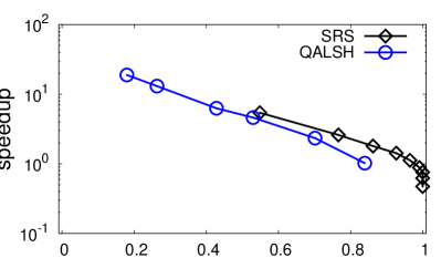
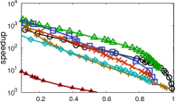
Figure 2 plots the trade-offs between the speedup and recall of two most recent data-independent algorithms SRS and QALSH on Sift and Audio. As both algorithms are originally external memory based approaches, we evaluate the speedup by means of the total number of pages of the dataset divided by the number of pages accessed during the search. It shows that SRS consistently outperforms QALSH. Table  2 shows the construction time and index size of SRS and QALSH, we can see that SRS has smaller index size than QALSH (at least 5 times larger than SRS). Thus, SRS is chosen as the representative in the second round evaluation where a cover-tree based in-memory implementation will be used.

(a) sift

(b) audio

Figure 2: Speedup vs Recall (Data-independent)

Table 2: index size and construction time (Data-independent)

Dataset	SRS		QALSH
	size(MB)	time(s)	size(MB)	time(s)
Audio	2.8	26.5	14.1	27.3
Sift	46.6	980	318	277
Notre	15.5	253.9	98.1	95.2
Sun	4.1	45.1	21.5	67.2

8.4.2 Encoding-based Methods

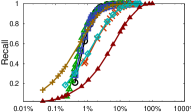
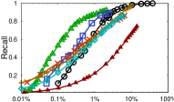
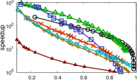
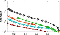
We evaluate six encoding based algorithms including OPQ, NAPP, SGH, AGH, NSH and SH. Figure 3 demonstrates that, of all methods, the search performance of OPQ beats other algorithms by a big margin on most of the datasets.

(a) Sift

(b) Trevi

(c) Mnist

(d) Glove

(e) Notre

(f) Ben

(g) Audio

(h) Cifa

Figure 3: Speedup vs Recall (Encoding)

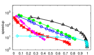
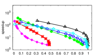
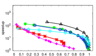
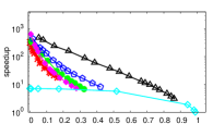
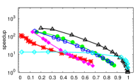
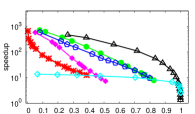
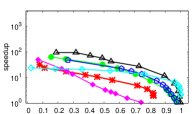
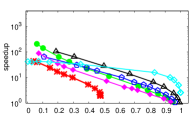
Table 3 reports the construction time (second) and index size (MB) of encoding-based methods. For most of datasets, NSH has the smallest index size, followed by AGH, SGH and OPQ. Selective Hashing has the largest index size because it requires long hash table to reduce the points number in a bucket and multiple hash tables to achieve high recall.

NSH and AGH spend relatively small time to build the index. The index time value of OPQ has a strong association with the length of the sub-codeword and dimension of the data point. Nevertheless, the index construction time of OPQ still turns out to be very competitive compared with other algorithms in the second round evaluation. Therefore, we choose OPQ as the representative of the encoding based methods.

Table 3: index size and construction time (Encoding)

Dataset	SH		OPQ		NAPP		NSH		AGH		SGH
	size	time	size	time	size	time	size	time	size	time	size	time
Sift	729	320	65	788.7	119	122	34.1	35.06	65	28	65.2	221
Trevi	185	132	158	10457	12	262	1.9	242.9	19.4	133	19.4	246
Mnist	165	34.5	11	152.4	8.3	35	2.4	96.4	4.6	26.9	6.9	358
Glove	850	375	43	697.7	143	119	77.3	105.9	78	20.6	41.3	89.4
Notre	325	107.2	17	138.4	40	39	16.5	28.2	11.9	5.3	22.3	206
Ben	792	352.3	68	844.6	131	134	37.7	38	38.2	16.8	71.9	447
Audio	155	18.1	9	45.8	6.4	8.4	1.8	24.8	3	8.1	4.6	360
Cifa	153	21.5	9	92.6	6	18.3	0.8	18.8	3.7	22	1.9	3

8.4.3 Tree-based Space Partition Methods

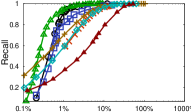
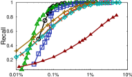
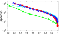
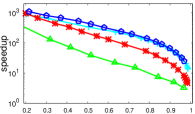
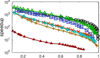
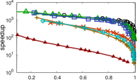
We evaluate three algorithms in this category: FLANN, Annoy and VP-tree. To better illustrate the performance of FLANN, we report the performance of both randomized kd-trees and hierarchical $k$-means tree, namely FLANN-KD and FLANN-HKM, respectively. Note that among $20$ datasets deployed in the experiments, the randomized kd-trees method (FLANN-KD) is chosen by FLANN in five datasets: Enron, Trevi, UQ-V, BANN and Gauss. The linear scan is used in the hardest dataset: Rand, and the hierarchical $k$-means tree (FLANN-HKM) is employed in the remaining $14$ datasets. Figure 4 shows that Annoy, FLANN-HKM and FLANN-KD can obtain the highest performance in different datasets.

(a) sift

(b) deep

(c) Enron

(d) Gist

(e) UQ-V

(f) Sun

(g) Audio

(h) Cifar

Figure 4: Speedup vs Recall (Tree-based)

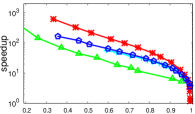
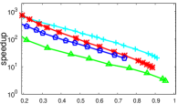
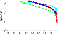
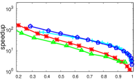
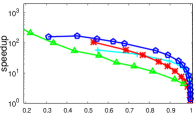
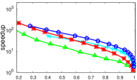
Note that the index size of VP-tree is the memory size used during the indexing. From table 4, we can see VP-Tree almost has the largest index time, which is because VP-tree spend long time to tune the parameters automatically. While the search performance of VP-tree is not competitive compared to FLANN and Annoy under all settings, it is excluded from the next round evaluation.

Table 4: index size and construction time (Tree-based)

Dataset	Annoy		Flann-KD		Flann-HKM		VP-tree
	size(MB)	time(s)	size(MB)	time(s)	size(MB)	time(s)	size(MB)	time(s)
Sift	572	144.6	274.0	45.5	230.0	27.4	573.1	131
Deep	571	224	550.0	148.6	74.0	1748.1	1063	474
Enron	56	51.1	27.0	30.0	74.0	412.9	500.7	954
Gist	563	544.9	540.0	462.9	1222.0	775.5	4177.6	1189
UQ-V	1753	801.8	1670.0	462.0	99.0	3109.2	3195.5	15.9
Sun	46	18.4	44.0	20.6	58.0	43.0	161	124
Audio	31	7.08	15.0	3.0	20.0	10.6	45	151
Cifa	28	10.8	14.0	7.0	9.0	23.7	101	131

8.4.4 Neighborhood-based Methods

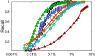
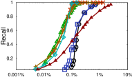
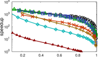
In the category of neighborhood-based methods, we evaluate four existing techniques: KGraph, SW, HNSW and RCT. Figure 5 shows that the search performance of KGraph and HNSW substantially outperforms that of other two algorithms on most of the datasets.

(a) Sift

(b) Nusw

(c) Audio

(d) Gist

(e) Deep

(f) Cifar

(g) Trevi

(h) Ben

Figure 5: Speedup vs Recall (Neighborhood-based)

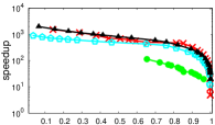
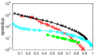
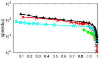
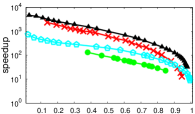
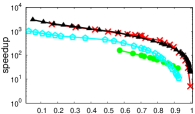
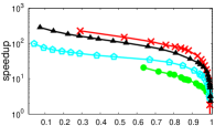
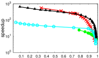
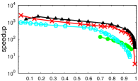
RCT has the smallest index size and the construction time of KGraph and HNSW are relatively large. Due to the outstanding search performance of KGraph and HNSW, we choose them as the representatives of the neighborhood-based methods. Note that we delay the comparison of DPG to the second round evaluation.

Table 5: index size and construction time (Neighborhood-based)

Dataset	HNSW		KGraph		SW		RCT
	size(MB)	time(s)	size(MB)	time(s)	size(MB)	time(s)	size(MB)	time(s)
Sift	589	1290	160	815.9	236	525	50	483
Nusw	541	701	44	913	64	605	22.1	813.9
Audio	45	36.9	9	38.2	13	8.1	2.4	11.8
Gist	3701	5090	158	6761.3	233	2994	50.3	3997
Deep	1081	1800	161	1527	236.5	372.1	51.2	815
Cifar	103	99.8	8	97.5	5.9	25.6	2.3	28
Trevi	1572	1292	16	1800.8	12.2	1003	4.5	649
Ben	651	1062	176	863	260	225	57	482

Figure 6: Speedup with Recall of $0.8$

Figure 7: Recall with Speedup of $50$

(a) Nusw

(b) Gist

(c) Glov

(d) Rand

(e) Msong

(f) Deep

(g) Sift

(h) Gauss

Figure 8: Speedup vs Recall on Different Datasets

(a) Nusw

(b) Gist

(c) Msong

(d) Deep

Figure 9: Recall vs Percentage of Data Points Accessed

Figure 10: The Ratio of Index Size and Data Size (%)

Figure 11: Index Construction Time (seconds)

8.5 Second Round Evaluation

In the second round evaluation, we conduct comprehensive experiments on seven representative algorithms: SRS, OPQ, FLANN, Annoy, HNSW, KGraph, and DPG.

8.5.1 Search Quality and Time

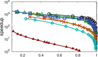
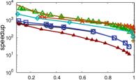
In the first set of experiments, Figure 6 reports the speedup of seven algorithms when they reach the recall around $0.8$ on $20$ datasets. Note that the speedup is set to $1.0$ if an algorithm cannot outperform the linear scan algorithm. Among seven algorithms, DPG and HNSW have the best overall search performance and KGraph follows. It is shown that DPG enhances the performance of KGraph, especially on hard datasets: Nusw, Gist, Glove and Rand. As reported thereafter, the improvement is also more significant on higher recall. For instance, DPG is ranked after KGraph on three datasets under this setting (recall $0.8$), but it eventually surpasses KGraph on higher recall. Overall, DPG and HNSW have the best performance for different datasets.

OPQ can also achieve a decent speedup under all settings. Not surprisingly, SRS is slower than other competitors with a huge margin as it does not exploit the data distribution. Similar observations are reported in Figure 7, which depicts the recalls achieved by the algorithms with speedup around $50$.

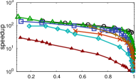
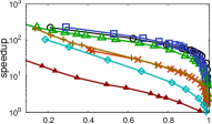
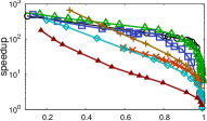
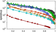
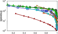
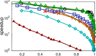
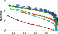
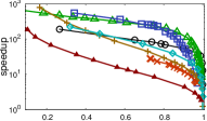
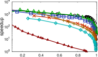
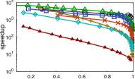
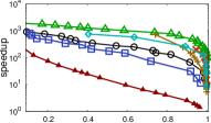
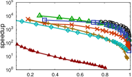
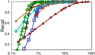
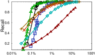
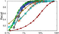
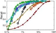
We evaluate the trade-off between search quality (Recall) and search time (Speedup and the percentage of data points accessed). The number of data points to be accessed ($N$) together with other parameters such as the number of trees (Annoy) and the search queue size (HNSW, KGraph and DPG), are tuned to achieve various recalls with different search time (i.e., speedup). Figure 8 illustrates speedup of the algorithms on eight datasets with recall varying from $0$ to $1$. It further demonstrates the superior search performance of DPG on high recall and hard datasets (Figure 8(a)-(d)). The overall performances of HNSW, KGraph and Annoy are also very competitive, followed by FLANN. It is shown that the performance of both DPG and KGraph are ranked lower than that of HNSW, Annoy, FLANN and OPQ in Figure 8(h) where the data points are clustered.

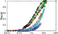
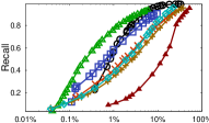
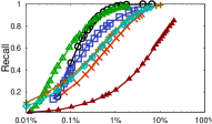
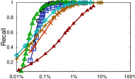
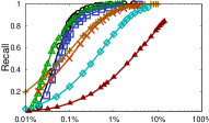
In Figure 9, we evaluate the recalls of the algorithms against the percentage of data points accessed, i.e., whose distances to the query in the data space are calculated. As the search of proximity-based methods starts from random entrance points and then gradually approaches the results while other algorithms initiate their search from the most promising candidates, the search quality of these methods is outperformed by Annoy, FLANN and even OPQ at the beginning stage. Nevertheless, their recall values rise up faster than other algorithms when more data points are accessed. Because of the usage of the hierarchical structure in HNSW, HNSW could approach the results more quickly.

8.5.2 Searching with Different $K$

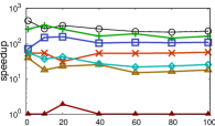
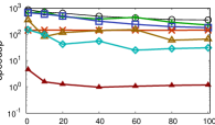
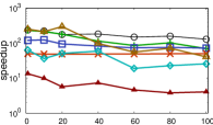
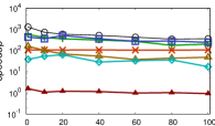
We evaluate the speedup at the recall of $0.8$ with different $K$. As shown in figure 12, DPG and HNSW almost has the best search performance for $K$ between 1 and 100, followed by KGraph and Annoy. The similar ranking could be observed in different $K$.

(a) Gist

(b) Sift

(c) MNIST

(d) Deep

Figure 12: Speedup with recall of 0.8 with Diff $K$

8.5.3 Index Size and Construction Time

In addition to search performance, we also evaluate the index size and construction time of seven algorithms on $20$ datasets. Figure 10 reports ratio of the index size (exclude the data points) and the data size. Except Annoy, the index sizes of all algorithms are smaller than the corresponding data sizes.

The index sizes of DPG, KGraph, HNSW and SRS are irrelevant to the dimensionality because a fixed number of neighbor IDs and projections are kept for each data point by neighborhood-based methods (DPG, KGraph and HNSW) and SRS, respectively. Consequently, they have a relatively small ratio on data with high dimensionality (e.g., Trevi). Overall, OPQ and SRS have the smallest index sizes, less than $5$% among most of the datasets, followed by HNSW, DPG, KGraph and FLANN. It is shown that the rank of the index size of FLANN varies dramatically over $20$ datasets because it may choose three possible index structures. Annoy needs to maintain a considerable number of trees for a good search quality, and hence has the largest index size.

Figure 11 reports the index construction time of the algorithms on $20$ datasets. SRS has the best overall performance due to its simplicity. Then Annoy ranks the second. The construction time of OPQ is related to the dimensionality because of the calculation of the sub-codewords (e.g., Trevi). HNSW, KGraph and DPG have similar construction time. Compared with KGraph, DPG doesn’t spend large extra time for the graph diversification. Nevertheless, they can still build the indexes within one hour for $16$ out of $20$ datasets.

8.5.4 Scalability Evaluation

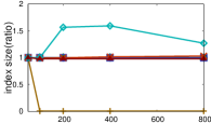
In Figure 13, we investigate the scalability of the algorithms in terms of the search time, index size and index construction time against the growth of the number of data points ($n$) and the dimensionality ($d$). The target recall is set to $0.8$ for evaluation of $n$ and $d$, respectively. Particularly, BANN is deployed with the number of data points growing from $1$M to $10$M. Following the convention, we use random data, Rand, to evaluate the impact of the dimensionality which varies from $50$ to $800$. To better illustrate the scalability of the algorithms, we report the growth ratio of the algorithms against the increase of $n$ and $d$. For instance, the index size growth ratio of DPG with $n=4M$ is obtained by its index size divided by the index size of DPG with $n=1M$.

(a) Vaying $n$, BANN

(b) Vaying $n$, BANN

(c) Vaying $n$, BANN

(d) Varying $d$, Rand

(e) Varying $d$, Rand

(f) Varying $d$, Rand

Figure 13: Scalability vs data size ($n$) and dim ($d$)

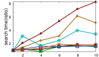
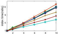
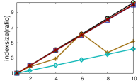
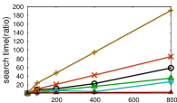
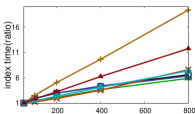
With the increase of the number of data points ($n$), DPG, KGraph, HNSW and Annoy have the best search scalability while SRS ranks the last. On the other hand, OPQ has the best scalability over index size and construction time, followed by FLANN. It is noticed that the performance of FLANN is rather unstable mainly because it chooses FLANN-KD when $n$ is $6$M and $10$M, and FLANN-HKM otherwise.

Regarding the growth of dimensionality, FLANN has the worst overall performance which simply goes for brute-force linear scan when $d\geq 100$. As expected, DPG, KGraph, HNSW and SRS have the best index size scalability since their index sizes are independent of $d$. It is interesting that SRS has the best search scalability, and its speedup even outperforms DPG when $d\geq 2000$. This is probably credited to its theoretical worse performance guarantee. Note that we do not report the performance of KGraph in Figure 13(d) because it is always outperformed by linear scan algorithm. This implies that KGraph is rather vulnerable to the high dimensionality, and hence justifies the importance of DPG, which achieves much better search scalability towards the growth of dimensionality.

8.5.5 Harder Query Workload

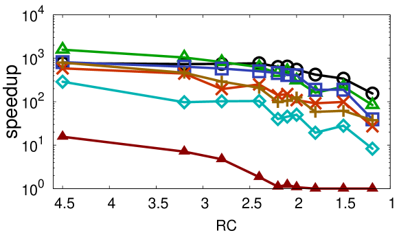
We evaluate the algorithm performances when the distribution of the query workload becomes different from that of the datasets. We control the generation of increasingly different query workloads by perturbing the default queries by a fixed length $\delta$ in a random direction. By increasingly large $\delta$ for the default queries on Sift, we obtain query workloads whose RC values vary from $4.5$ (without perturbation) to $1.2$. Intuitively, queries with smaller RC values are harder as the distance of a random point in the dataset and that of the NN point becomes less distinguishable. Figure 14 shows the speedups of the algorithms with recall at around $0.8$ on the harder query workloads characterized by the RC values. The speedups of all the algorithms decrease with the increase of RC values. HNSW has the best performance on easy queries, followed by DPG, KGraph, Annoy and FLANN. Nevertheless, DPG is the least affected and still achieves more than 100x speedup (with a recall at least 0.8) on the hardest settings. This demonstrates the robustness of DPG against different query workloads.

(a) Speedup with Recall of $0.8$

Figure 14: Queries with Different RC Values (Sift)

8.6 Summary

Table 6 ranks the performances of the seven algorithms from various perspectives including search performance, index size, index construction time, and scalability. We also indicate that SRS is the only one with theoretical guarantee of searching quality, and it is very easy to tune the parameters for search quality and search time. The tuning of Annoy is also simple, simply varying the number of the trees. It is much complicated to tune the parameters of FLANN. Authors therefore developed the auto-configure algorithm to handle this.

Below are some recommendations for users according to our comprehensive evaluations.

• When there are sufficient computing resources (both main memory and CPUs) for the off-line index construction, and sufficient main memory to hold the resulting index, DPG and HNSW are the best choices for ANNS on high dimensional data due to their outstanding search performance in terms of robustness to the datasets, result quality, search time and search scalability.

  We also recommend Annoy, due to its excellent search performance, and robustness to the datasets. Additionally, a nice property of Annoy is that, compared with proximity graph based approaches, it can provide better trade-off between search performance and index size/construction time. This is because, one can reduce the number of trees without hurting the search performance substantially.

  Note that KGraph also provides overall excellent performance except on few datasets (e.g., the four hard datasets and Yout). We recommend Annoy instead of KGraph as DPG is an improved version of KGraph with better performance, and Annoy performs best in the few cases where both DPG and KGraph do not perform as well (e.g., Yout, and Gauss).

• To deal with large scale datasets (e.g., $1$ billion of data points) with moderate computing resources, OPQ and SRS are good candidates due to their small index sizes and construction time. It is worthwhile to mention that, SRS can easily handle the data points updates and have theoretical guarantee, which distinguish itself from other five algorithms.

Category	Search Performance	Index		Index Scalabiliity		Search Scalabiliity		Theoretical Guarantee	Tuning Difficulty
		Size	Time	Datasize	Dim	Datasize	Dim
DPG	1st	4th	7th	=4th	=1st	=1st	5th	No	Medium
HNSW	1st	3rd	5th	=4th	4th	=1st	4th	No	Medium
KGraph	3rd	5th	6th	=4th	=1st	=1st	7th	No	Medium
Annoy	4th	7th	2nd	7th	3rd	6th	=2nd	No	Easy
FLANN	5th	6th	4th	=2nd	7th	=1st	6th	No	Hard
OPQ	6th	2nd	3rd	1st	=5th	5th	=2nd	No	Medium
SRS	7th	1st	1st	=2nd	=5th	7th	1st	Yes	Easy

Table 6: Ranking of the Algorithms Under Different Criteria

9 Further Analyses

In this section, we analyze the most competitive algorithms in our evaluations, grouped by category, in order to understand their strength and weakness.

9.1 Space Partition-based Approach

Our comprehensive experiments show that Annoy, FLANN and OPQ have the best performance among the space partitioning-based methods. Note that FLANN chooses FLANN-HKM in most of the datasets. Therefore, all three algorithms are based on k-means space partitioning.

We identify that a key factor for the effectiveness of k-means-style space partitioning is that the large number of clusters, typically $\Theta(n)$. Note that we cannot directly apply k-means with $k=\Theta(n)$ because (i) the index construction time complexity of k-means is linear to $k$, and (ii) the time complexity to identify the partition where the query is located takes $\Theta(n)$ time. Both OPQ and FLANN-HKM/Annoy achieve this goal indirectly by using the ideas of subspace partitioning and recursion, respectively.

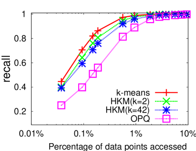
We perform experiments to understand which idea is more effective. We consider the goal of achieving k-means-style space partitioning with approximately the same number of partitions. Specifically, we consider the following choices: (i) Use k-means directly with $k=18,611$. (ii) Use OPQ with $2$ subspaces and each has 256 clusters. The number of effective partitions (i.e., non-empty partitions) is also $18,611$. (iii) Use FLANN-HKM with branching factor $L=2$ and $L=42$, respectively. We also modify the stopping condition so that the resulting trees have $18,000$ and $17,898$ partitions, respectively. Figure 15(a) reports the recalls of the above choices on Audio against the percentage of data points accessed. Partitions are accessed ordered by the distances of their centers to the query. We can see that OPQ-based partition has the worst performance, followed by (modified) FLANN-HKM with $L=42$, and then $L=2$. k-means has the best performance, although the performance differences between the latter three are not significant. Therefore, our analysis suggests that hierarchical k-means-based partitioning is the most promising direction so far.

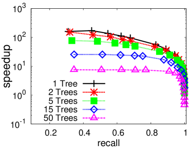
Our second analysis is to investigate whether we can further boost the search performance by using multiple hierarchical k-means trees. Note that Annoy already uses multiple trees and it significantly outperforms a single hierarchical k-means tree in FLANN-HKM on most of the datasets. It is natural to try to enhance the performance of FLANN-HKM in a similar way. We set up an experiment to construct multiple FLANN-HKM trees. In order to build different trees, we perform k-means clustering on a set of random samples of the input data points. Figure 15(b) shows the resulting speedup vs recall where we use up to 50 trees. We can see that it is not cost-effective to apply multiple trees for FLANN-HKM on Audio, mainly because the trees obtained are still similar to each other, and hence the advantage of multiple trees cannot offset the extra indexing and searching overheads. Note that Annoy does not suffer from this problem because $2$-means partition with limited number of samples and iterations naturally provides diverse partitions.

(a) Partition Quality

(b) Multiple HKM Trees

Figure 15: Analyses of Space Partitioning-based Methods

9.2 Neighborhood-based Approach

(a) Min # of hops to any 20-NNs (Yout)

(b) Min # of hops to any 20-NNs (Gist)

Figure 16: minHops Distributions of KGraph and DPG

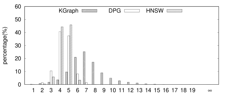
Our first analysis is to understand why KGraph, DPG and HNSW work very well (esp. attaining a very high recall) in most of the datasets. Our preliminary analysis indicates that this is because (i) the $k$NN points of a query are typically closely connected in the neighborhood graph, and (ii) most points are well connected to at least one of the $k$NN points of a query. (ii) means there is a high empirical probability that one of the $p$ entry points selected randomly by the search algorithm can reach one of the $k$NN points, and (i) ensures that most of the $k$NN points can be returned. By well connected, we mean there are many paths from an entry point to one of the $k$NN point, hence there is a large probability that the “hills” on one of the path is low enough so that the search algorithm won’t stuck in the local minima.

We also investigate why KGraph does not work well on some datasets and why DPG and HNSW works much better. KGraph does not work on Yout and Gauss mainly because both datasets have many well-separated clusters. Hence, the index of KGraph has many disconnected components. Thus, unless one of the entrance points used by its search algorithm is located in the same cluster as the query results, there is no or little chance for KGraph to find any near point. On the other hand, mainly due to the diversification step and the use of the reverse edges in DPG, there are edges linking points from different clusters, hence resulting in much improved recalls. Similarly, in HNSW, the edges are also well linked.

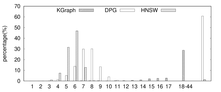
For example, we perform the experiment where we use the NN of the query as the entrance point of the search on Yout. KGraph then achieves 100% recall. In addition, we plot the distribution of the minimum number of hops (minHops) for a data point to reach any of the $k$NN points of a query for the indexes of KGraph and DPG on Yout and Gist in Figure 16. We can observe that

• For KGraph, there are a large percentage of data points that cannot reach any $k$NN points (i.e., those corresponding to $\infty$ hops) on Yout (60.38%), while the percentage is low on Gist (0.04%).

• The percentages of the $\infty$ hops are much lower for DPG (1.28% on Yout and 0.005% on Gist).

• There is no $\infty$ hops for HNSW on both datasets.

• DPG and HNSW have much more points with small minHops than KGraph, which contributes to making it easier to reach one of the $k$NN points. Moreover, on Yout, HNSW has the most points with small minHops over three algorithms, which results in a better performance as shown in Figure 8(g).

9.3 Comparisions with Prior Benchmarks

We have verified that the performance results obtained in our evaluation generally match prior evaluation results, and we can satisfactorily explain most of the few discrepancies.

Comparison with ann-benchmark’s Results.   While the curves in both evaluations have similar shapes, the relative orders of the best performing methods are different. This is mainly due to the fact that we turned off all hardware-specific optimizations in the implementations of the methods. Specifically, we disabled distance computation using SIMD and multi-threading in KGraph, -ffast-math compiler option in Annoy, multi-threading in FLANN, and distance computation using SIMD, multi-threading, prefetching technique and -Ofast compiler option in methods implemented in the NonMetricSpaceLib, i.e., SW, NAPP, VP-tree and HNSW). In addition, we disabled the optimized search implementation used in HNSW. We confirm that the results resemble ann-benchmark’s more when these optimizations are turned on.

Disabling these hardware-specific optimizations allows us to gain more insights into the actual power of the algorithms. In fact, the optimizations can be easily added to the implementations of all the algorithms.

KGraph and SW.   KGraph was ranked very low in the ann-benchmark study [8] possibly due to an error in the test.

Annoy.   We note that the performance of latest version of Annoy (based on randomized hierarchical $2$-means trees) is noticeably better than its earlier versions (based on multiple heuristic RP-trees), and this may affect prior evaluation results.

10 CONCLUSION AND FUTURE WORK

NNS is an fundamental problem with both significant theoretical values and empowering a diverse range of applications. It is widely believed that there is no practically competitive algorithm to answer exact NN queries in sublinear time with linear sized index. A natural question is whether we can have an algorithm that empirically returns most of the $k$NN points in a robust fashion by building an index of size $O(n)$ and by accessing at most $\alpha n$ data points, where $\alpha$ is a small constant (such as 1%).

In this paper, we evaluate many state-of-the-art algorithms proposed in different research areas and by practitioners in a comprehensive manner. We analyze their performances and give practical recommendations.

Due to various constraints, the study in this paper is inevitably limited. In our future work, we will (i) use larger datasets (e.g., $100$M+ points); (ii) consider high dimensional sparse data; (iii) use more complete, including exhaustive method, to tune the algorithms; (iv) consider other distance metrics, as in [34].

Finally, our understanding of high dimensional real data is still vastly inadequate. This is manifested in many heuristics with no reasonable justification, yet working very well in real datasets. We hope that this study opens up more questions that call for innovative solutions by the entire community.

Appendix A Parameter Setting

In this section, we carefully tune all algorithms to achieve a good search performance with reasonable index space and construction time overheads. By default, we use the number of data points verified (i.e., computing the exact distance to the query), denoted by $N$, to achieve the trade-off between the search quality and search speed unless specially mentioned.

A.1 SRS

We test SRS in two versions: External-Memory version and In-Memory version. In this paper, we do not use the early termination test and stop the searching when it has accessed enough points. Meanwhile, the approximation ratio $c$ is set to 4 and the page size for external memory version is $4096$. For the sake of fairness, the success probability of all data-independent methods is set to $1/2-1/e$. Therefore, there are two parameters $T^{\prime}$(the maximum number of data points accessed in the query processing), $m$ (the number of dimension of projected space) for SRS algorithm. We change the number of the accessed data points to tune the trade-off between the search quality and search speed under a certain $m$.

External-Memory Version

Figure 17 plots the changes of the search performance with different projection dimensions. As the increase of the projection dimensionality $m$, SRS could achieve a better performance.

(a) Audio

(b) Sift

Figure 17: IO Speedup vs Recall for Diff $m$ (Ex-Memory SRS)

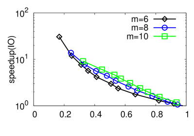
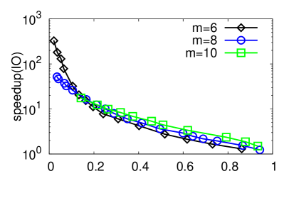
In-Memory version

For In-Memory version, we compare the speedup using the ratio of the brute-force time and the search time. From figure 18, we can see as the increase of the value of $m$, higher speedup could be achieved for high recall while the search speed would be more faster when one requires a relatively moderate value of recall. Considering various aspects, values of $m$ from 8 to 10 provide a good trade-off.

(a) Audio

(b) Sift

(c) Mnist

(d) Gist

Figure 18: Speedup vs Recall for Diff $m$ (In-Memory SRS)

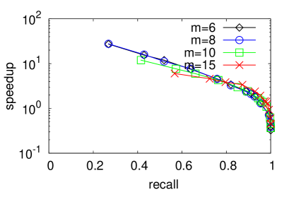
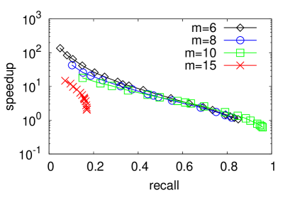
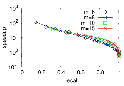
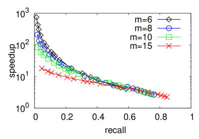
A.2 QALSH

Because QALSH didn’t release the source code of In-Memory version, we only test the performance of External-Memory version. We use the default setting for QALSH and tune the value of $c$(approximation ratio) to obtain different search performance.

(a) Audio

(b) Sift

Figure 19: IO Speedup vs Recall for QALSH

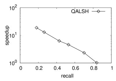
A.3 Scalable Graph Hashing

In SGH, we use the default setting recommended by the author. For kernel feature construction, we use Gaussian kernel and take 300 randomly sampled points as kernel bases. Hence, we compare the search accuracies with different hashcode length $b$. For most of the datasets, $b=8$ always obtains the worst search performance compared with larger hashcodes and the best speedup could be achieved with 128 bits.

(a) Audio

(b) Cifa

(c) Deep

(d) Yout

Figure 20: Speedup vs Recall for Diff $b$ (SGH)

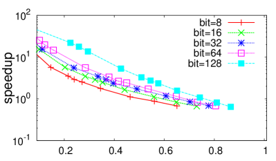
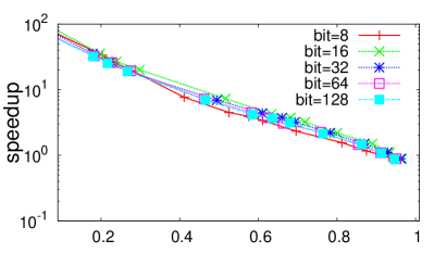
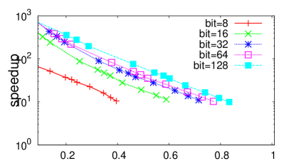
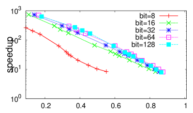
A.4 Anchor Graph Hashing

To run 1-AGH and 2-AGH, we have to fix three parameters: $m$ (the number of anchor), $s$ (number of nearest anchors need to be considered for each point) and hash code length $b$. We focus $m$ to 300 and $s$=5.

Following are the comparisons for 1-AGH and 2-AGH. We first show the search performance for a single-layer AGH and two-layer AGH with different length of hashcode. For most datasets, it seems using longer hashcode could obtain the much higher performance. Hence, we only compare the performance for $b=64$ and $b=128$ on both layer AGH. We can observe that 2-AGH provides superior performance compared to 1-AGH for majority of datasets.

(a) Sift for 1-AGH

(b) Yout for 1-AGH

(c) Sift for 2-AGH

(d) Yout for 2-AGH

Figure 21: Speedup vs Recall for Diff $b$ (AGH)

(a) Sift

(b) Yout

Figure 22: Speedup vs Recall for 1-AGH and 2-AGH

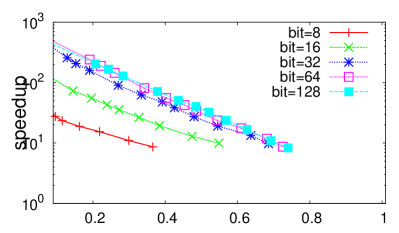
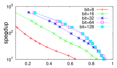
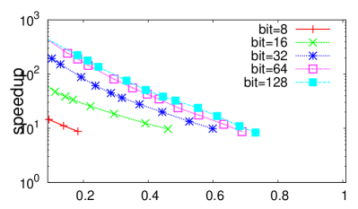
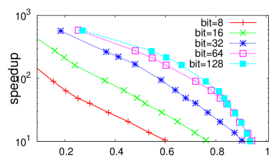
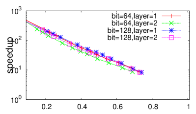
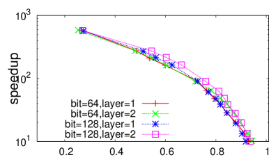
A.5 Neighbor-Sensitive Hashing

we set the number of pivots $m$ to $4b$ where $b$ is the length of hash code and used k-means++ to generate the pivots as described by the authors. The value of $\eta$ was set to 1.9 times of the average distance from a pivot to its closest pivot. We tune the value of $b$ to get the best performance.

(a) Audio

(b) Sift

(c) Sun

(d) Trevi

Figure 23: Speedup vs Recall for Diff $b$ (NSH)

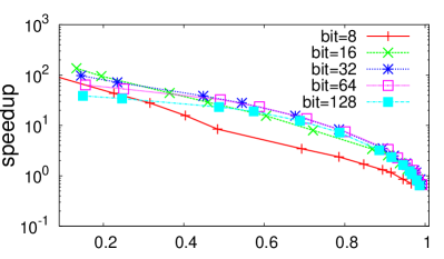
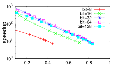
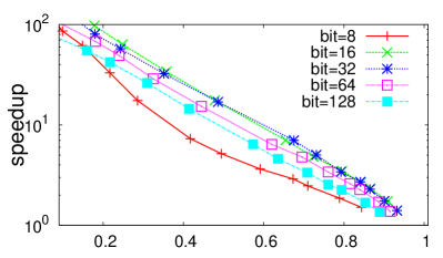
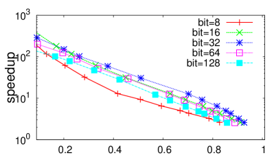
A.6 NAPP

Tunning NAPP involves selection of three parameters: $PP$ (the total number of pivots), $P_{i}$ (the number of indexed pivots) and $P_{s}$(the number of the shared pivots with the query). According to the experiments in [34], the values of $PP$ between 500 and 2000 provide a good trade-off. The large value of $PP$ will take long construction time. We will tune the value of $PP$ from 500 to 2000. The author also recommend the value of $P_{i}$ to be 32. We will change $P_{s}$ to get different search performance.

(a) Audio

(b) Sift

(c) Deep

(d) Glove

Figure 24: Speedup vs Recall for Diff $m$ (NAPP)

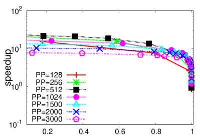
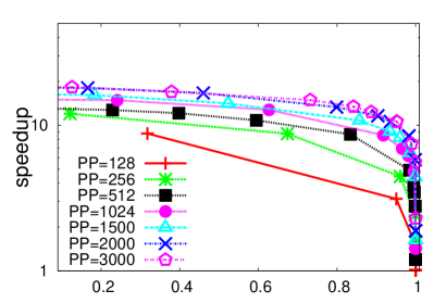
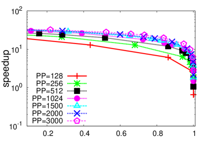
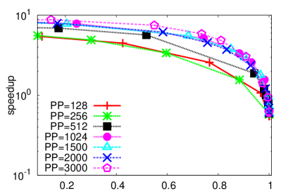
A.7 Selective Hashing

The experimentation was performed with the default parameter settings provided by the authors. The total number of buckets of per table is 9973. The number of radii $\mathcal{G}$ is set to 20. We change the number of the retrieved points $T$ and the approximation ratio $c$ to get different recalls.

(a) Sift

(b) Mnist

Figure 25: Speedup vs Recall for Diff $c$ (SH)

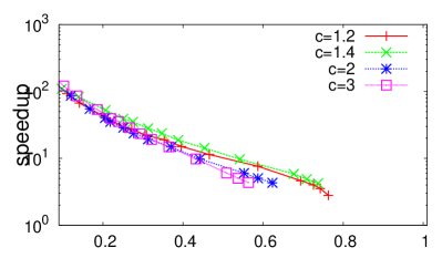
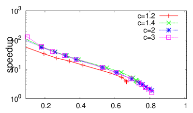
A.8 OPQ

An optimized product quantizer with $M$ subspaces and $k$ sub-codeword in each is used to build inverted multi-index. The product quantizer is optimized using the non-parametric solution initialized by the natural order. The OPQ is generated using $M=2$ and evaluates at most $T$ data points to obtain different search trade-off. For most of the datasets, $k=10$ would achieve a good performance while $k=8$ would be better for the datasets with small data points.

(a) Audio

(b) Sift

(c) Gist

(d) Nusw

Figure 26: Speedup vs Recall for Diff $k$ (OPQ)

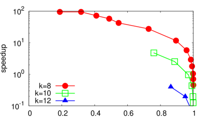
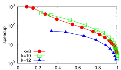
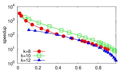
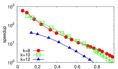
A.9 VP-tree

In NonMetricSpaceLibrary, VP-tree uses a simple polynomial pruner to generate the optimal parameters $\alpha_{left}$ and $\alpha_{right}$. We use auto-tuning procedure to produce different search performance by given the input parameter $target$ (which is the expected recall) and $b$ (the maximum number of points in leaf nodes).

(a) imageNet

(b) Sift

(c) Deep

(d) Glove

Figure 27: Speedup vs Recall for Diff $b$ (VP-tree)

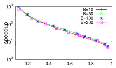
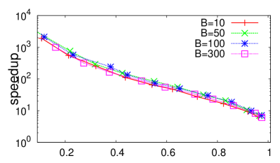
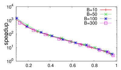
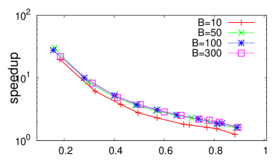
A.10 Annoy

Annoy only involves one parameter: trees number $f$. Table 7 and 8 shows the index sizes and the construction time complexities are linear to $f$. The search performance could be significantly improved by using multiple Annoy trees while the growth rate changes slowly when $f$ is larger than $50$ for most of the datasets.Considering the search performance and index performance comprehensively, we build $50$ trees for all the datasets.

Name	$1$Tree	$10$Trees	$50$Trees	$100$Trees	$200$Trees
Audio	0.04	0.5	2.3	4.5	9.4
Yout	2.3	22.1	112.6	217	442
Sift	1.8	17	85	128	352
Gauss	8.2	77	384	608	1538

Table 7: construction time using different trees

Name	$1$Tree	$10$Trees	$50$Trees	$100$Trees	$200$Trees
Audio	40.5	45.9	70	100	160.1
Yout	2347	2382	2539	2735	3128
Sift	512	612	1058	1615	2730
Gauss	3960	4161	5055	6171	8407

Table 8: index size using different trees

(a) Audio

(b) Sift

(c) Yout

(d) Gauss

Figure 28: Speedup vs Recall for Diff $f$ (Annoy)

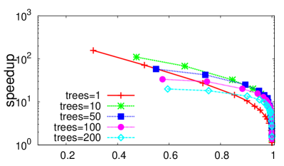
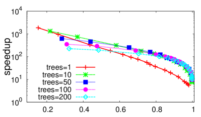
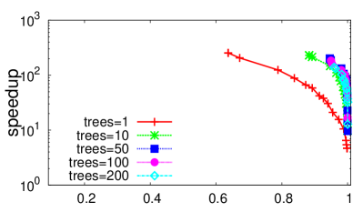
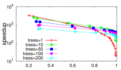
A.11 HKMeans

We randomly select the init centers in the k-means clustering. According to the recommendations from the source code of Flann, we apply different combinations of iteration times $iter$ and branching size $b$ to generate the recall-speedup trade-off.

(a) Sift with branches=64

(b) sift with branches=128

Figure 29: Speedup vs Recall for Diff $iter$ (Flann-HKM)

(a) Sift

(b) UQ_V

Figure 30: Speedup vs Recall for Diff $b$ (Flann-HKM)

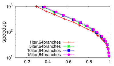
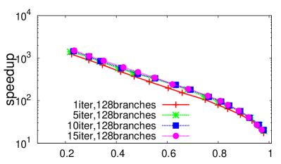
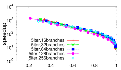
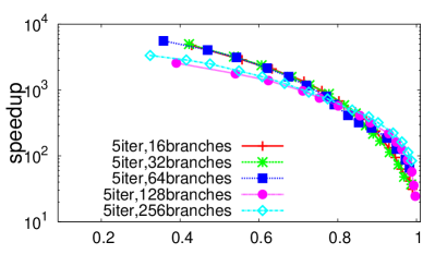
A.12 KDTree

Except the parameter $t$ which is the number of Randomized kdtrees, we use the default setting provided by the source code. The search performance would be improved as the growth of the number of trees. While the speedup doesn’t show considerable increase when $t$ is larger than 8.

(a) Audio

(b) Deep

(c) Sift

(d) Gist

Figure 31: Speedup vs Recall for Diff $t$ (Flann-KD)

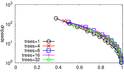
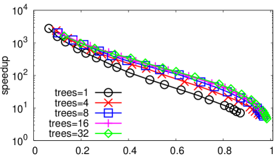
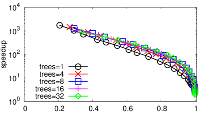
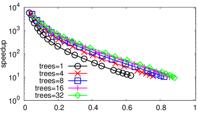
A.13 Flann

Flann defines the cost as a combination of the search time, tree build time and the tree memory overhead.

We used the default search precisions (90 percent) and several combinations of the tradeoff factors $wb$ and $wm$. For the build time weight, $wb$, we used three different possible values: 0 representing the case where we don’t care about the tree build time, 1 for the case where the tree build time and search time have the same importance and 0.01 representing the case where we care mainly about the search time but we also want to avoid a large build time. Similarly, the memory weight was chosen to be 0 for the case where the memory usage is not a concern, 100 representing the case where the memory use is the dominant concern and 1 as a middle ground between the two cases.

When we pay more attention to the size of the memory use, the search speedup is very low and almost declines to that of linear scan. For the datasets who have the medium data size or the system with enough memory, the $wm$ of 0 would provide a good search performance. Due to the large margin between large $wb$ and small $wb$ for the search performance, we select $0.01$ for $wb$ in this paper.

(a) Sift

(b) Mnist

Figure 32: Speedup vs Recall for Diff $wm$ (Flann)

(a) Sift

(b) Mnist

Figure 33: Speedup vs Recall for Diff $wb$ (Flann)

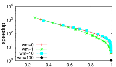
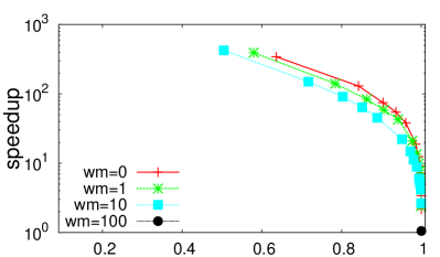
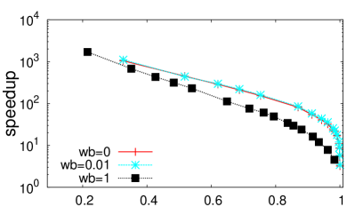
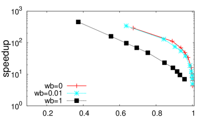
A.14 Small World

Small World involves the parameter NN( NN closest points are found during index constructing period). $S$ (number of entries using in searching procedure) is a searching parameter and we tune the value of $S$ to obtain the trade-off between the search speed and quality. The construction algorithm is computationally expensive and the time is roughly linear to the value of $NN$. Figure 34 shows the speedup with different $NN$. The small value of $NN$ could provide a good search performance for low recall but decrease for high recall. For most of datasets, the algorithm could provide a good search tradeoff when $NN$ is 10 or 20.

(a) Ben

(b) Deep

(c) MSong

(d) Glove

Figure 34: Speedup vs Recall for Diff $NN$(SW)

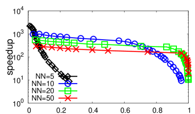
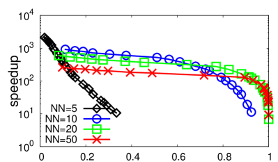
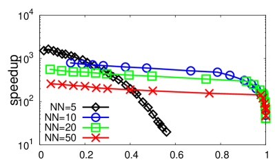
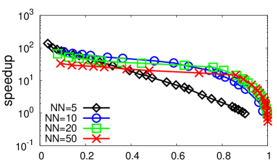
A.15 Hierarchical Navigable Small World

Two main parameters are adopted to get the tradeoff between the index complexity and search performance: $M$ indicates the size of the potential neighbors in some layers for indexing phase, and $efConstruction$ is used to controlled the quality of the neighbors during indexing. We use the default value of $efConstruction$, which is set to 200. $efSearch$ is a parameter similar to $efConstruction$ to control the search quality. We change the value of $efSearch$ to get the tradeoff between the search speed and quality. Figure 35 show the search performance of different $M$. Similar to SW, the small value of $M$ could provide a good search performance for low recall but decrease for high recall. We set $M=10$ as a default value.

(a) Sift

(b) Deep

(c) MNIST

(d) Ben

Figure 35: Speedup vs Recall for Diff $M$(HNSW)

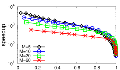
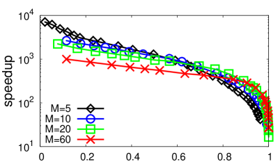
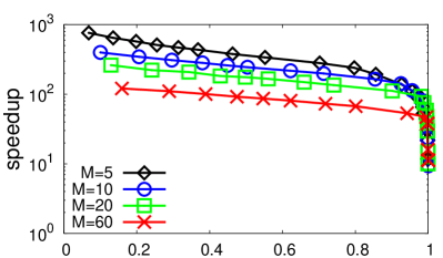
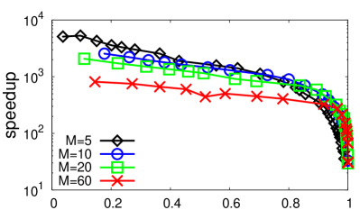
A.16 Rank Cover Tree

In RCT, there are parameters: $\Delta$($1/\Delta$ is the sample rate sampled from the lower level, which could determine the height $h$ of the tree), $p$(the maximum number of parents for each node) and coverage parameter $\omega$.Acording to the the recommendations from the authors, we select $h=4$ to build the rank cover tree.

(a) Sift for Diff $p$

(b) Nusw for Diff $p$

(c) Sift for Diff $\omega$

(d) Nusw for Diff $\omega$

Figure 36: Speedup vs Recall (RCT)

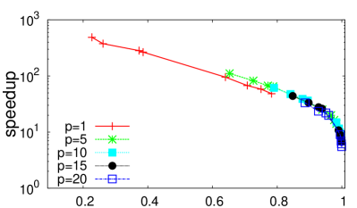
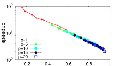
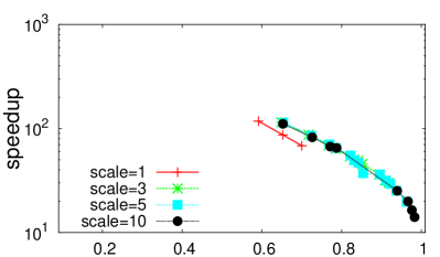
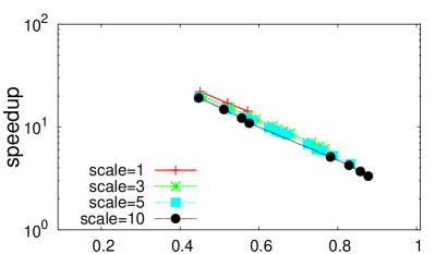
A.17 KGraph

K-NN Graph involves three parameters: $IK$ (the number of most similar objects connected with each vertex), sample rate $\rho$, termination threshold $\zeta$ and $P$ (initial entries count to start the search). The meaning of $\zeta$ is the loss in recall tolerable with early termination. We use a default termination threshold of 0.002. As reported by the author, the recall grows slowly beyond $\rho=0.5$. Here we study the impact of $IK$ and $\rho$ on performance. From figure 37, we see that $K>40$ is need for most of the datasets.

(a) Audio

(b) Sift

(c) Mnist

(d) Notre

Figure 37: Speedup vs Recall for Diff $L$ (KGraph)

A.18 DPG

The parameter tuning of DPG is similar to that of KGraph. In the experiments, DPG has the same setting with KGraph except that we use $\kappa=\frac{K}{2}=20$ so that the index size of DPG is the same as that of KGraph in the worst case.

Figure 38 shows that using count based diversification (i.e., DPG_C ) achieves similar search performance as using angular similarity based diversification (i.e., DPG_O).

(a) Sift

(b) Gist

(c) Imag

(d) Notre

(e) Ben

(f) Nus

Figure 38: Speedup vs Recall between counting-based DPG and angular-based DPG

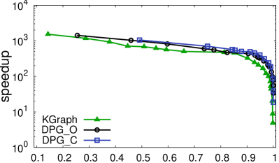
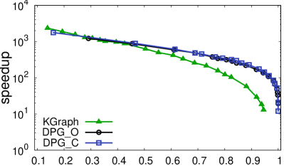
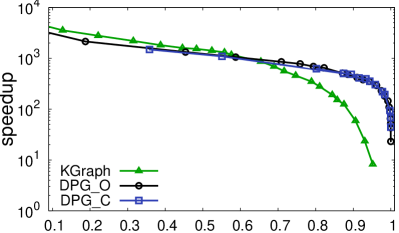
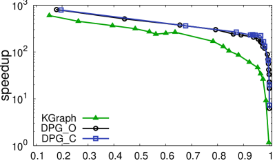
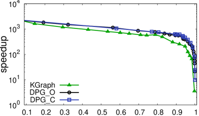
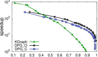
Figure 39 shows the comparisons of the diversification time between counting-based DPG and angular-based DPG. DPG_C spends more less time than DPG_O. The improvements are especially significant for the dataset with large data points.

Figure 39: diversification time between DPG_C and DPG_O

A.19 Default setting

Below are the default settings of the key parameters of the algorithms in the second round evaluation in Section 8.5.

• SRS. The number of projections ($m$) is set to $8$.

• OPQ. The number of subspaces is $2$, and each subspace can have $2^{10}$ codewords (i.e., cluster centers) by default.

• Annoy. The number of the Annoy trees, $m$, is set to $50$.

• FLANN. We let the algorithm tune its own parameters.

• HNSW. The number of the connections for each point, $M$, is set to $10$.

• KGraph. By default, we use $K=40$ for the K-NN graph index.

• DPG. We use $\kappa=\frac{K}{2}=20$ so that the index size of DPG is the same as that of KGraph in the worst case.

Appendix B Supplement for the Second Round Evaluation

Figure 40 and 41 show the trade-off between search quality(Recall) and search time(Speedup and the percentage of data points to be accessed) for the remaining datasets(some have been shown in 8.5).

(a) audio

(b) cifar

(c) enron

(d) imag

(e) Mnist

(f) Notre

(g) Sun

(h) Trevi

(i) Ben

(j) UQ-V

(k) Yout

(l) BANN

Figure 40: Speedup vs Recall

(a) audio

(b) cifar

(c) enron

(d) imag

(e) Glove

(f) Rand

(g) Sift

(h) Gauss

(i) Mnist

(j) Notre

(k) Sun

(l) Trevi

(m) Ben

(n) UQ-V

(o) Yout

(p) BANN

Figure 41: Recall vs Percentage of Data Points Accessed

References

- [1] L. Amsaleg, O. Chelly, T. Furon, S. Girard, M. E. Houle, K. Kawarabayashi, and M. Nett. Estimating local intrinsic dimensionality. In SIGKDD, 2015.
- [2] A. Andoni, P. Indyk, T. Laarhoven, I. P. Razenshteyn, and L. Schmidt. Practical and optimal LSH for angular distance. CoRR, abs/1509.02897, 2015.
- [3] A. Andoni and I. Razenshteyn. Optimal data-dependent hashing for approximate near neighbors. In STOC, 2015.
- [4] F. André, A. Kermarrec, and N. L. Scouarnec. Cache locality is not enough: High-performance nearest neighbor search with product quantization fast scan. PVLDB, 9(4):288–299, 2015.
- [5] K. Aoyama, K. Saito, H. Sawada, and N. Ueda. Fast approximate similarity search based on degree-reduced neighborhood graphs. In SIGKDD, 2011.
- [6] A. Babenko and V. S. Lempitsky. The inverted multi-index. In CVPR, pages 3069–3076, 2012.
- [7] E. Bernhardsson. Annoy at github https://github.com/spotify/annoy, 2015.
- [8] E. Bernhardsson. Benchmarking nearest neighbors https://github.com/erikbern/ann-benchmarks, 2016.
- [9] A. Beygelzimer, S. Kakade, and J. Langford. Cover trees for nearest neighbor. In ICML, pages 97–104, 2006.
- [10] L. Boytsov and B. Naidan. Learning to prune in metric and non-metric spaces. In NIPS, 2013.
- [11] S. Brin. Near neighbor search in large metric spaces. In VLDB, pages 574–584, 1995.
- [12] R. Caruana, N. Karampatziakis, and A. Yessenalina. An empirical evaluation of supervised learning in high dimensions. In ICML, pages 96–103, 2008.
- [13] S. Dasgupta and Y. Freund. Random projection trees and low dimensional manifolds. In STOC, 2008.
- [14] M. Datar, N. Immorlica, P. Indyk, and V. S. Mirrokni. Locality-sensitive hashing scheme based on p-stable distributions. In SoCG, 2004.
- [15] W. Dong. Kgraph. http://www.kgraph.org, 2014.
- [16] W. Dong, M. Charikar, and K. Li. Efficient k-nearest neighbor graph construction for generic similarity measures. In WWW, 2011.
- [17] K. Fukunaga and P. M. Narendra. A branch and bound algorithms for computing k-nearest neighbors. IEEE Trans. Computers, 24(7):750–753, 1975. hierachical k-means tree.
- [18] J. Gan, J. Feng, Q. Fang, and W. Ng. Locality-sensitive hashing scheme based on dynamic collision counting. In SIGMOD, 2012.
- [19] J. Gao, H. V. Jagadish, B. C. Ooi, and S. Wang. Selective hashing: Closing the gap between radius search and k-nn search. In SIGKDD, 2015.
- [20] T. Ge, K. He, Q. Ke, and J. Sun. Optimized product quantization. IEEE Trans. Pattern Anal. Mach. Intell., 36(4):744–755, 2014.
- [21] R. M. Gray and D. L. Neuhoff. Quantization. IEEE Transactions on Information Theory, 44(6):2325–2383, 1998.
- [22] J. He, S. Kumar, and S. Chang. On the difficulty of nearest neighbor search. In ICML, 2012.
- [23] M. E. Houle and M. Nett. Rank-based similarity search: Reducing the dimensional dependence. IEEE TPAMI, 37(1):136–150, 2015.
- [24] M. E. Houle and J. Sakuma. Fast approximate similarity search in extremely high-dimensional data sets. In ICDE, pages 619–630, 2005.
- [25] Q. Huang, J. Feng, Y. Zhang, Q. Fang, and W. Ng. Query-aware locality-sensitive hashing for approximate nearest neighbor search. PVLDB, 9(1):1–12, 2015.
- [26] P. Indyk and R. Motwani. Approximate nearest neighbors: Towards removing the curse of dimensionality. In STOC, 1998.
- [27] H. Jégou, M. Douze, and C. Schmid. Product quantization for nearest neighbor search. IEEE Trans. Pattern Anal. Mach. Intell., 33(1):117–128, 2011.
- [28] Q. Jiang and W. Li. Scalable graph hashing with feature transformation. In IJCAI, pages 2248–2254, 2015.
- [29] C.-C. Kuo, F. Glover, and K. S. Dhir. Analyzing and modeling the maximum diversity problem by zero-one programming*. Decision Sciences, 24(6):1171–1185, 1993.
- [30] W. Liu, J. Wang, S. Kumar, and S. Chang. Hashing with graphs. In ICML, pages 1–8, 2011.
- [31] Y. Malkov, A. Ponomarenko, A. Logvinov, and V. Krylov. Approximate nearest neighbor algorithm based on navigable small world graphs. Inf. Syst., 45:61–68, 2014.
- [32] Y. A. Malkov and D. A. Yashunin. Efficient and robust approximate nearest neighbor search using hierarchical navigable small world graphs. CoRR, 2016.
- [33] M. Muja and D. G. Lowe. Scalable nearest neighbor algorithms for high dimensional data. IEEE Trans. Pattern Anal. Mach. Intell., 36(11):2227–2240, 2014.
- [34] B. Naidan, L. Boytsov, and E. Nyberg. Permutation search methods are efficient, yet faster search is possible. PVLDB, 8(12):1618–1629, 2015.
- [35] Y. Park, M. J. Cafarella, and B. Mozafari. Neighbor-sensitive hashing. PVLDB, 9(3):144–155, 2015.
- [36] M. Radovanovic, A. Nanopoulos, and M. Ivanovic. Hubs in space: Popular nearest neighbors in high-dimensional data. Journal of Machine Learning Research, 11:2487–2531, 2010.
- [37] G. Schindler, M. A. Brown, and R. Szeliski. City-scale location recognition. In CVPR, 2007.
- [38] C. Silpa-Anan and R. I. Hartley. Optimised kd-trees for fast image descriptor matching. In CVPR, 2008.
- [39] Y. Sun, W. Wang, J. Qin, Y. Zhang, and X. Lin. SRS: solving c-approximate nearest neighbor queries in high dimensional euclidean space with a tiny index. PVLDB, 8(1):1–12, 2014.
- [40] Y. Sun, W. Wang, Y. Zhang, and W. Li. Nearest neighbor search benchmark https://github.com/DBWangGroupUNSW/nns_benchmark, 2016.
- [41] J. Wang, W. Liu, S. Kumar, and S. Chang. Learning to hash for indexing big data - A survey. Proceedings of the IEEE, 104(1):34–57, 2016.
- [42] J. Wang, H. T. Shen, J. Song, and J. Ji. Hashing for similarity search: A survey. CoRR, abs/1408.2927, 2014.
- [43] R. Weber, H.-J. Schek, and S. Blott. A quantitative analysis and performance study for similarity-search methods in high-dimensional spaces. In A. Gupta, O. Shmueli, and J. Widom, editors, VLDB, 1998.
- [44] P. N. Yianilos. Data structures and algorithms for nearest neighbor search in general metric spaces. In SODA, pages 311–321, 1993.
- [45] J. Zhai, Y. Lou, and J. Gehrke. Atlas: a probabilistic algorithm for high dimensional similarity search. In SIGMOD, 2011.