Janus Collaboration

A statics-dynamics equivalence through the fluctuation-dissipation ratio provides a window into the spin-glass phase from nonequilibrium measurements

Abstract

The unifying feature of glass formers (such as polymers, supercooled liquids, colloids, granulars, spin glasses, superconductors, …) is a sluggish dynamics at low temperatures. Indeed, their dynamics is so slow that thermal equilibrium is never reached in macroscopic samples: in analogy with living beings, glasses are said to age. Here, we show how to relate experimentally relevant quantities with the experimentally unreachable low-temperature equilibrium phase. We have performed a very accurate computation of the non-equilibrium fluctuation-dissipation ratio for the three-dimensional Edwards-Anderson Ising spin glass, by means of large-scale simulations on the special-purpose computers Janus and Janus II. This ratio (computed for finite times on very large, effectively infinite, systems) is compared with the equilibrium probability distribution of the spin overlap for finite sizes. The resulting quantitative statics-dynamics dictionary, based on observables that can be measured with current experimental methods, could allow the experimental exploration of important features of the spin-glass phase without uncontrollable extrapolations to infinite times or system sizes.

Theory and Experiment follow apparently diverging paths when studying the glass transition. On the one hand, experimental glass formers (spin glasses, fragile molecular glasses, polymers, colloids, …) undergo a dramatic increase of characteristic times when cooled down to their glass temperature, $T_{\mathrm{g}}$ Cavagna (2009). Below $T_{\mathrm{g}}$, the glass is always out of equilibrium and aging appears Vincent et al. (1997). Consider a rapid quench from a high temperature to the working temperature $T$ ($T<T_{\mathrm{g}}$), where the system is left to equilibrate for time $t_{\mathrm{w}}$ and probed at a later time $t+t_{\mathrm{w}}$. Response functions such as the magnetic susceptibility turn out to depend on $t/t_{\mathrm{w}}^{\mu}$, with $\mu\approx 1$ Vincent et al. (1997); Rodriguez et al. (2003); Dupuis et al. (2005). The age of the glass, $t_{\mathrm{w}}$, remains the relevant time scale even for $t_{\mathrm{w}}$ as large as several days. Relating the aging experimental responses to equilibrium properties is an open problem.

A promising way to fill the gap is to establish a statics-dynamics dictionary (SDD) Barrat and Berthier (2001); Belletti et al. (2008a); Baños et al. (2010a, b): non-equilibrium properties at finite times $t$, $t_{\mathrm{w}}$, as obtained on samples of macroscopic size $L\to\infty$, are quantitatively matched to equilibrium quantities computed on systems of finite size $L$ [the SDD is an $L\leftrightarrow(t,t_{\mathrm{w}})$ correspondence]. Clearly, in order for it to be of any value, an SDD cannot strongly depend on the particular pair of aging and equilibrium quantities that are matched.

Some time ago, we proposed one such a SDD Belletti et al. (2008a); Baños et al. (2010a, b). However, this SDD was unsatisfactory in two respects. First, $L$ was matched only to $t_{\mathrm{w}}$ (irrespectively of the probing time $t+t_{\mathrm{w}}$). Second, our SDD matched spatial correlation functions whose experimental study is only incipient Oukris and Israeloff (2010); Komatsu et al. (2011).

One could think Barrat and Berthier (2001) of building an SDD through the Generalized Fluctuation Dissipation relations (GFDR) first introduced in Cugliandolo and Kurchan (1993) (for related developments see Franz and Rieger (1995); Marinari et al. (1998); Franz et al. (1998, 1999); Marinari et al. (2000a); Hérisson and Ocio (2002); Cruz et al. (2003); Hérisson and Ocio (2004)). The GFDR are correct at very large times. However, on time scales that can be investigated in experiments, glassy systems are not fully thermalized since the approach to equilibrium is very slow. Strong corrections pollute GFDR at finite times. Here we show how the SDD can be used in a particular case to compute such corrections (that will be likely present in all glassy systems). We find that the naive implementation of this idea Barrat and Berthier (2001) does not work in general, and we introduce a modified SDD that works for spin glasses (and, hopefully, also for glasses).

GFDR carry crucial information Cugliandolo and Kurchan (1993); Franz et al. (1998, 1999): they provide a promising experimental path towards measuring Parisi’s functional order parameter Parisi (1979). As a consequence GFDR have attracted much attention. One encounters numerical studies for both Ising Marinari et al. (1998, 2000a); Cruz et al. (2003) and Heisenberg Kawamura (2003); Billoni et al. (2005) spin glasses, as well as for structural glasses Parisi (1997); Barrat and Kob (1999); Barrat and Berthier (2000); Berthier (2007); Gnan et al. (2013). On the experimental side, we have studies on atomic spin glasses Hérisson and Ocio (2002, 2004), superspin glasses Komatsu et al. (2011), polymers Grigera and Israeloff (1999); Oukris and Israeloff (2010), colloids Bellon et al. (2001); Maggi et al. (2010, 2012); Gomez-Solano et al. (2009); Jop et al. (2009); Greinert et al. (2006); Bonn and Kegel (2003) or DNA Dieterich et al. (2015).

Here, we perform a detailed simulation of GFDR in the three-dimensional Ising spin glass employing the custom-made supercomputers Janus Belletti et al. (2008b) and Janus II Baity-Jesi et al. (2014). In fact, this has been the launching simulation campaign of the Janus II machine, which was designed with this sort of dynamical studies in mind. Our simulations stand out by the spanned time range (11 orders of magnitude), by our high statistical accuracy and by the range of system sizes, enabling us to control size effects ($L=20,\ 40,\ 80$ and $160$). Thus armed, we assess whether or not an SDD can be built from the GFDR, and compare the SDD proposed in this paper with other proposals. We focus on spin glasses, rather than on other model glasses, for a number of reasons: (i) their sluggish dynamics is known to be due to a thermodynamic phase transition at $T_{\mathrm{c}}=T_{\mathrm{g}}$ Gunnarsson et al. (1991); Palassini and Caracciolo (1999); Ballesteros et al. (2000); (ii) the linear size of the magnetically correlated domains, $\xi(t_{\mathrm{w}})$, is experimentally accessible Joh et al. (1999); Bert et al. (2004) ($\xi\sim 100$ lattice spacings Joh et al. (1999), much larger than comparable measurements for structural glasses Berthier et al. (2005)); (iii) a GFDR-based SDD has been well established in the limit of large sizes and times Cugliandolo and Kurchan (1993); Franz et al. (1998, 1999), see (4) below; (iv) GFDR have been studied experimentally Hérisson and Ocio (2002); (v) well developed, yet mutually contrasting, theoretical scenarios are available for spin glasses in equilibrium Young (1998); (vi) magnetic systems are notably easier to model and to simulate numerically (in fact, special-purpose computers have been built for the simulation of spin glasses Cruz et al. (2001); Ogielski (1985); Belletti et al. (2008b, 2009a); Baity-Jesi et al. (2014)).

GFDR and the SDD

We suddenly cool a three-dimensional spin-glass sample of size $L^{3}$ from high temperature to the working (sub-critical) temperature $T=0.7=0.64T_{\mathrm{c}}$ at the initial time $t_{\mathrm{w}}=0$ (see Methods, below, for more details and definitions). During the non-equilibrium relaxation a coherence length $\xi(t_{\mathrm{w}}$) grows Joh et al. (1999); Belletti et al. (2008a, 2009b), which is representative of the size of the spin-glass domains. Then, from the waiting time $t_{\mathrm{w}}$ on, we place the system under a magnetic field of strength $H$, and consider the response function at a later measuring time $t+t_{\mathrm{w}}$

$$\chi_{L}(t+t_{\mathrm{w}},t_{\mathrm{w}})=\left.\frac{\partial m_{L}(t+t_{\mathrm{w}})}{\partial H}\right|_{H=0},$$ (1)

where $m_{L}(t+t_{\mathrm{w}})$ is the magnetization density in a sample of linear size $L$. This susceptibility is then compared with the spin temporal correlation function $C_{L}(t+t_{\mathrm{w}},t_{\mathrm{w}})$. From now on, we shall take the limits

$$\chi(t+t_{\mathrm{w}},t_{\mathrm{w}}) =\lim_{L\to\infty}\chi_{L}(t+t_{\mathrm{w}},t_{\mathrm{w}})\,,$$ (2)

$$C(t+t_{\mathrm{w}},t_{\mathrm{w}}) =\lim_{L\to\infty}C_{L}(t+t_{\mathrm{w}},t_{\mathrm{w}})\,,$$ (3)

which are easy to control numerically: if $L\gtrsim 7\xi(t+t_{\mathrm{w}})$ size effects are negligible Belletti et al. (2008a) (see also Appendix F).

The Fluctuation Dissipation Theorem (FDT) states that $T\chi(t+t_{\mathrm{w}},t_{\mathrm{w}})=1-C(t+t_{\mathrm{w}},t_{\mathrm{w}})$, with both $\chi$ and $C$ computed at $H=0$. However, for $T<T_{\mathrm{c}}$ the FDT does not hold. In fact, GFDR take the form Cugliandolo and Kurchan (1993); Franz et al. (1998, 1999) (the order of limits is crucial):

$$\lim_{t_{\mathrm{w}}\to\infty}T\chi(t+t_{\mathrm{w}},t_{\mathrm{w}})=\lim_{t_{\mathrm{w}}\to\infty}[\lim_{L\to\infty}S(C_{L}(t+t_{\mathrm{w}},t_{\mathrm{w}}),L)]\,,$$ (4)

where $t$ is scaled as $t_{\mathrm{w}}$ grows, to ensure that the full range $0<C(t+t_{\mathrm{w}},t_{\mathrm{w}})<1$ gets covered, and $S(C,L)$ is given by a double integral of $P(q,L)$, the equilibrium distribution function of the spin overlap, whose explicit definition is provided in the Methods Section.

Here, we mimic an experimental protocol Hérisson and Ocio (2002, 2004) in that we consider the non-equilibrium response on a very large system but at finite times. We try to relate this response with the equilibrium overlap for a system of finite effective size $L_{\mathrm{eff}}$

$$T\chi(t+t_{\mathrm{w}},t_{\mathrm{w}})=S\big{(}C(t+t_{\mathrm{w}},t_{\mathrm{w}}),L_{\mathrm{eff}}(t+t_{\mathrm{w}},t_{\mathrm{w}})\big{)}\,,$$ (5)

where we have assumed that both $\chi$ and $C$ have reached their thermodynamic limit. The same approach was followed for a two-dimensional spin glass by Barrat and Berthier Barrat and Berthier (2001) (note, however, that there is no stable spin-glass phase at $T>0$ in two spatial dimensions).

Eq. (5) provides a statics-dynamics dictionary (SDD) relating both times $t$ and $t_{\mathrm{w}}$ with a single effective equilibrium size $L_{\mathrm{eff}}(t+t_{\mathrm{w}},t_{\mathrm{w}})$. Note that it is not obvious a priori that our program can be carried out. For instance, our SDD does not exist for ferromagnets, as explained in details in Appendix H exploiting data from Refs. Parisi et al. (1999); Ricci-Tersenghi (2003).

SDDs based on the comparison of aging and equilibrium correlation functions (rather than on GFDR) have been studied in some detail Baños et al. (2010a, b); Fernández and Martín-Mayor (2015). It was found that the effective length depends solely on $t_{\mathrm{w}}$. Indeed,

$$L_{\mathrm{eff}}(t+t_{\mathrm{w}},t_{\mathrm{w}})=k\,\xi(t_{\mathrm{w}})\,,$$ (6)

with $k\approx 3.7$, was accurate enough to match the correlation functions Baños et al. (2010a, b). Ref. Barrat and Berthier (2001) also agreed with (6). In fact, (6) also underlies the analysis of Refs.  Manssen et al. (2015); Wittmann and Young (2016). Yet, we shall show below that (6) is oversimplified.

Figure 1: Response function $T\chi(t+t_{\mathrm{w}},t_{\mathrm{w}})$ versus $C(t+t_{\mathrm{w}},t_{\mathrm{w}})$ at $T=0.7$ [for fixed $t_{\mathrm{w}}$, $C(t+t_{\mathrm{w}},t_{\mathrm{w}})$ monotonically decreases from $C=1$ at $t=0$ to $C=0$ at $t=\infty$]. Data for $t_{\mathrm{w}}=2^{11}$ and $t_{\mathrm{w}}=2^{30}$ were obtained on Janus II (the other $t_{\mathrm{w}}$ are from Janus). The five values of $t_{\mathrm{w}}$ correspond to effective equilibrium sizes $L_{\mathrm{eff}}$ that, according to (6), span the size range investigated in Ref. Baños et al. (2010a) (namely, $8\leq L\leq 32$). Inset: growth of the spin-glass coherence length $\xi(t_{\mathrm{w}})$ as a function of time, computed at zero magnetic field and following Refs. Belletti et al. (2008a, 2009b), from simulations of $L=160$ lattices at $T=0.7$ on Janus II. In dashed lines we plot the scaling $\xi(t_{\mathrm{w}})\propto t_{\mathrm{w}}^{1/z(T)}$ with $z(T)=11.64$ from Ref. Belletti et al. (2009a).

Numerical data

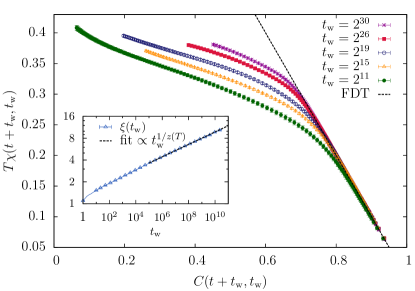
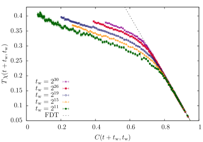
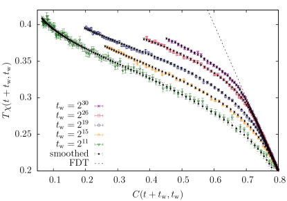
The three basic quantities computed in this work, namely $\chi(t+t_{\mathrm{w}},t_{\mathrm{w}}),C(t+t_{\mathrm{w}},t_{\mathrm{w}})$ and $\xi(t_{\mathrm{w}})$ are displayed in Fig. 1. Full details about this computation are provided in Appendix C.

Let us remark that the Janus II supercomputer allows us to probe unexplored dynamical regimes, either $t/t_{\mathrm{w}}$ as large as $2^{24}\approx 1.4\times 10^{7}$ (i.e., we follow the magnetic response for a very long time, after the field was switched on at $t_{\mathrm{w}}=2^{11}$) or $t_{\text{w}}$ as large as $2^{30}$ (i.e., we study the response of a very old spin glass, but we are limited to $t/t_{\mathrm{w}}\approx 27$ in this case).

It is also remarkable that we are able to compute both the susceptibility $\chi$ and the correlation function $C$ without worrying about finite-size effects. Indeed, size effects become visible when the coherence length reaches the threshold $\xi(t_{\mathrm{w}})\approx L/7$ Belletti et al. (2008a) which in our $L=160$ lattice translates to $\xi\approx 23$ lattice spacings. As Fig. 1–inset shows, we are quite far from this safety threshold.

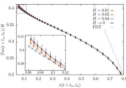
With respect to previous measurements of the GFDR ratio, it is worth stressing that now we are able to take the $h\to 0$ limit in a more controlled way. This is far from trivial, given that the linear response regime shrinks to very small field when $t_{\mathrm{w}}$ increases (see Appendix C).

The data in Fig. 1 also stand out by their statistical accuracy (due to the large number of samples and large system sizes we simulated, but also thanks to the analysis method described in Appendix D As a consequence, a behavior different from the one implied by FDT, $T\chi(t,t_{\mathrm{w}})=1-C(t,t_{\mathrm{w}})$ can be studied in detail. In particular, the reader might be stricken by the linear behavior at $C(t+t_{\mathrm{w}},t_{\mathrm{w}})\approx 0.4$. In fact, following Refs. Cugliandolo and Kurchan (1993); Franz et al. (1998, 1999), this linear behavior could be interpreted as evidence for one step of replica-symmetry breaking (see, for instance, Ref. Mézard et al. (1987)). However, we shall argue below that the effective length in (5) evolves as time $t$ grows, thus producing an upturn in the response which is probably responsible for the linear behavior in Fig. 1.

Let us make a final remark. We know that $S(C,L)$ is upper bounded by $1-\overline{\langle|q|\rangle}_{L=\infty}\geq 1-q_{\mathrm{EA}}^{(L=\infty)}$ (see Methods for definitions; the proof of the inequality is outlined in Appendix G. At $T=0.7$ we know that $1-q_{\mathrm{EA}}^{(L=\infty)}=0.48(3)$ Baños et al. (2010b) (or 0.46(3) Baños et al. (2010a)). Therefore, the dynamic responses $T\chi(t,t_{\mathrm{w}})$ in Fig. 1 are well below $1-q_{\mathrm{EA}}^{(L=\infty)}$ and (5) could be satisfied. The general conditions under which (5) can be used are discussed in the Appendix.

Figure 2: Close-up of Fig. 1 (we only show data for three $t_{\mathrm{w}}$, for the sake of clarity). Lines are $S(C,L_{\mathrm{eff}})$, recall (5), with the effective equilibrium size as in (6): $L_{\mathrm{eff}}(t+t_{\mathrm{w}},t_{\mathrm{w}})=k\xi(t_{\mathrm{w}})$. Dotted lines correspond to $k=3.7$, which is the proportionality constant that was found by matching equilibrium and non-equilibrium correlation functions Belletti et al. (2008a); Baños et al. (2010a, b). The continuous lines were found by choosing the best possible $k$ for each $t_{\mathrm{w}}$. This representation shows that the single-time statics-dynamics dictionary $L_{\text{eff}}\sim\xi(t_{\mathrm{w}})$ breaks down for large $t$, when $\xi(t+t_{\mathrm{w}})$ is much larger than $\xi(t_{\mathrm{w}})$.

Figure 3: For each $t_{\mathrm{w}}$, we show the effective equilibrium size $L_{\mathrm{eff}}(t+t_{\mathrm{w}},t_{\mathrm{w}})$ in units of the coherence length at the measuring time $\xi(t+t_{\mathrm{w}})$ versus the ratio of coherence lengths $\xi(t+t_{\mathrm{w}})/\xi(t_{\mathrm{w}})$ (recall that $t$ is the time elapsed since switching-on the magnetic field). The ratio of coherence lengths is 1 for $t=0$ and goes as $\xi(t+t_{\mathrm{w}})/\xi(t_{\mathrm{w}})\propto(1+t/t_{\mathrm{w}})^{1/z(T)}$ for large time, with $z(T=0.7)=11.64(15)$ Belletti et al. (2009b). Let us stress that there is no extrapolation in this figure, only interpolation (i.e., $L_{\text{eff}}$ falls within the simulated equilibrium sizes, $8\leq L_{\mathrm{eff}}\leq 32$). The solid line is a fit to the scaling function $h(x)$ in (7) and (9). Inset: $L_{\mathrm{eff}}(t+t_{\mathrm{w}},t_{\mathrm{w}})$ data from the main panel in units of the coherence length at the initial time time $\xi(t_{\mathrm{w}})$, as a function of the time ratio $t/t_{\mathrm{w}}$.

The effective equilibrium size

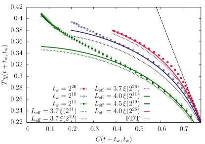
As we show in Fig. 2, our data are too accurate to be quantitatively described by combining (5) with (6). This simple description fails both at short times $t$ (i.e., when $C(t,t_{\mathrm{w}})\approx q_{\mathrm{EA}}^{[L\approx 4\xi(t_{\mathrm{w}})]}$) and also at very long $t$, although one can find a constant $k$ that works well for intermediate $t$.

The discrepancy for long $t$ seems easy to rationalize: since the growth of $\xi(t_{\mathrm{w}})$ is very slow, recall Fig. 1–inset, $\xi(t+t_{\mathrm{w}})$ and $\xi(t_{\mathrm{w}})$ are very similar to each other for small $t$ and, therefore, $L_{\mathrm{eff}}\propto\xi(t_{\mathrm{w}})$ makes sense. However, since $\xi(t_{\mathrm{w}})$ grows without bounds in the spin-glass phase, one should eventually have $\xi(t+t_{\mathrm{w}})\gg\xi(t_{\mathrm{w}})$. Under these circumstances, it is only natural that $L_{\mathrm{eff}}\propto\xi(t+t_{\mathrm{w}})$.

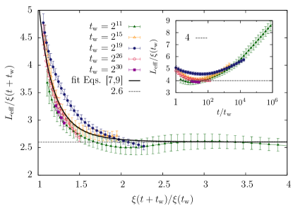
We can test this proposal by computing an exact $L_{\text{eff}}$ for each $(t,t_{\mathrm{w}})$ pair (see Appendix E for details), which we plot in Fig. 3: in the main panel in units of $\xi(t+t_{\mathrm{w}})$ and in the inset in units of $\xi(t_{\mathrm{w}})$.

The first important observation from the main panel in Fig. 3 is that, for long enough times, we find $L_{\mathrm{eff}}\approx 2.6\,\xi(t+t_{\mathrm{w}})$, in agreement with the intuition exposed above. This is definitely different from (6), used until now. The data in the inset of Fig. 3 explain why the previous relation in (6) passed many numerical tests until now: the non-monotonic behavior of $L_{\mathrm{eff}}/\xi(t_{\mathrm{w}})$ for short times $t$ makes this ratio roughly compatible with a constant $k\approx 4$ as long as $t/t_{\mathrm{w}}\lesssim 1000$.

Surprisingly, the ratio $L_{\mathrm{eff}}/\xi(t+t_{\mathrm{w}})$, or equivalently $L_{\mathrm{eff}}/\xi(t_{\mathrm{w}})$, becomes large as well when $t\to 0$, thus explaining the inability of (5) in describing dynamical data at short times $t$ (see Fig. 2). Nonetheless in the limit $t\to 0$, i.e. $\xi(t+t_{\mathrm{w}})/\xi(t_{\mathrm{w}})\to 1$, the effective equilibrium size $L_{\mathrm{eff}}$ seems to reach a finite value; a divergence of $L_{\mathrm{eff}}$ in this limit seems unlikely (see Appendix I).

$L_{\mathrm{eff}}$ and the spin-glass coherence length

Now that it is clear that both $\xi(t_{\mathrm{w}})$ and $\xi(t+t_{\mathrm{w}})$ are relevant for $L_{\mathrm{eff}}$ one may ask about the crossover between the $\xi(t_{\mathrm{w}})$-dominated regime and the $\xi(t+t_{\mathrm{w}})$-dominated regime. Fig. 3 tells us that $L_{\mathrm{eff}}/\xi(t+t_{\mathrm{w}})$ is, to a good approximation, a function of the ratio $\xi(t+t_{\mathrm{w}})/\xi(t_{\mathrm{w}})$. Thus, we attempted to fit the crossover with the functional form

$$L_{\mathrm{eff}}(t+t_{\mathrm{w}},t_{\mathrm{w}})=\xi(t+t_{\mathrm{w}})\,h\big{(}\xi(t+t_{\mathrm{w}})/\xi(t_{\mathrm{w}})\big{)}\,,$$ (7)

where the scaling function is

$$h(x)=k_{1}\ +\ k_{2}\,x^{-c}\,.$$ (8)

Interpolation of data shown in Fig. 3 returns: $k_{1}=2.58(2)$, $k_{2}=2.7(1)$ and $c=5.9(2)$. Noticing that $k_{2}\approx k_{1}$ and $c\approx z(T)/2$, where $z(T)$ is the exponent for the time growth of the coherence length, $z(T=0.7)=11.64(15)$ (see Fig. 1–inset, and Refs. Belletti et al. (2008a, 2009b)), the scaling function $h(x)$ can be also rewritten in a much simpler form as

$$h\big{(}\xi(t+t_{\mathrm{w}})/\xi(t_{\mathrm{w}})\big{)}=k_{1}\left(1+\sqrt{\frac{t_{\mathrm{w}}}{t+t_{\mathrm{w}}}}\right)$$ (9)

Fitting data in Fig. 3 with this simpler scaling function returns $k_{1}=2.59(1)$ (see full curve in Fig. 3). Given that the fit with 3 adjustable parameters in (8) and the one in (9) with just 1 adjustable parameter have practically the same quality-of-fit, we tend to prefer the simpler ansatz, as long as it interpolates the numerical data well enough.

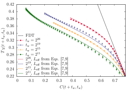
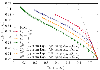
The ultimate check for the success of (7) and (9) in reproducing the aging response is provided by Fig. 4, where the dynamical measurements (data points with errors) are plotted together with the equilibrium function $S(C(t+t_{\mathrm{w}},t_{\mathrm{w}}),L_{\mathrm{eff}}(t+t_{\mathrm{w}},t_{\mathrm{w}}))$. The very good agreement in the whole range gives a strong support in favor of an SDD based on (7) and (9).

Note as well that (7) explains the previous success of the simpler SDD in (6). In fact, at short times $t$, the two coherence lengths $\xi(t+t_{\mathrm{w}})$ and $\xi(t_{\mathrm{w}})$ are very similar to each other, and the amplitude $k$ in (6) is essentially $k=k_{1}+k_{2}\approx 2k_{1}$.

The ansatz of (7) provides as well a simple explanation for the upturn of the aging response at small values of $C$, recall Fig. 1. Indeed, as time $t$ increases, the correlation function decays as $C\propto(t+t_{\mathrm{w}})^{-1/\alpha},\alpha\approx 7$ Belletti et al. (2008a). But, from $\xi(t+t_{\mathrm{w}})\propto(t+t_{\mathrm{w}})^{1/z(T)}$ we conclude that, even at fixed $t_{\mathrm{w}}$, $L_{\mathrm{eff}}$ diverges for large $t$ as $C^{-\alpha/z(T)}$. Now, to a first approximation, one may expect that $S(C,L=\infty)-S(C,L)\propto L^{-\theta\approx-0.38}$ (see the description of the overlap distribution function in the Methods section, below). We thus expect the susceptibility to approach its $C=0$ limit in a singular way, as $C^{\theta/(\alpha z(T))}\approx C^{0.23}$.

Figure 4: As in Fig. 2 but $L_{\mathrm{eff}}$ is taken from the ansatz in (7) and (9), which improves on the single-time statics-dynamics dictionary based on $\xi(t_{\mathrm{w}})$ by considering a crossover to a $\xi(t+t_{\mathrm{w}})$-dominated regime.

Which features of the $P(q)$ can be obtained from dynamic measurements?

One of the major gains of the present analysis would be to obtain Parisi’s functional order parameter $P(q)$ from experimental dynamic data. In an ideal situation, one would have data for $\chi$, $C$ and $\xi$, complemented by the ansatz in (9). Then, one would like to know which features of the underlying $S(C,L)$ can be retrieved from these dynamic measurements.

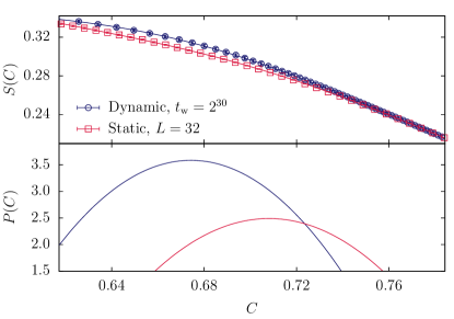
In order to answer this question, we have considered a very simplified $P_{\mathrm{simpl}}(q,L)$, that possesses the main features of the $P(q,L)$ measured in numerical simulations (see Methods):

$$P_{\mathrm{simpl}}(q,L)= \,\big{(}P_{0}+P_{1}q^{2}\big{)}\,\mathbbm{1}\big{[}|q|<q_{\mathrm{EA}}^{(L)}\big{]}+$$

$$w^{(L)}\big{(}\delta(q-q_{\mathrm{EA}}^{(L)})+\delta(q+q_{\mathrm{EA}}^{(L)})\big{)}/2\,,$$ (10)

where $P_{0}$ and $P_{1}$ are constants, $\mathbbm{1}$ is the indicator function and $w^{(L)}$ is a weight enforcing normalization. Integrating $P_{\mathrm{simpl}}(q,L)$ twice we get

$$S_{\mathrm{simpl}}(C,L)=\min\left[S_{0}(L)-P_{0}C^{2}-\frac{P_{1}}{6}C^{4},1-C\right]\,.$$ (11)

We take $S_{0}(L)=S(0,L)$ from the true $P(q,L)$. Recall that $S(0,L)=1-\overline{\langle|q|\rangle}_{L}$, see Appendix G. Instead, the $L$-independent $P_{0}$ and $P_{1}$ are fitted in order to obtain a $S_{\mathrm{simpl}}(C,L)$ as similar as possible to the true $S(C,L)$: we get $P_{0}=0.167(1)$ and $P_{1}=0.46(3)$. In other words, $P_{\mathrm{simpl}}(q)$ shares with the true distribution only four numeric features: normalization, first absolute moment $\overline{\langle|q|\rangle}_{L}$, $P_{0}\simeq P(q=0,L)$ which is essentially $L$-independent, and the second derivative $P_{1}\simeq P^{\prime\prime}(q=0,L)/2$. In particular, note that having $P_{0}>0$ is a crucial feature of the mean-field solution Marinari et al. (2000b). A direct measure for sizes $8\leq L\leq 32$ returns the $L$-independent value $P(q=0,L)=0.167(5)$ Baños et al. (2010a) confirming the validity of our simplified description.

The outcome of this analysis is given in Fig. 5. It turns out that the simplified $S_{\mathrm{simpl}}$ in (11) is almost as effective as the true $S(C,L)$ in representing the non-equilibrium data through the effective size $L_{\mathrm{eff}}$ in (9). The only obvious disagreement is that (11) predicts a non-analytic behavior for the susceptibility $\chi$ at $C=q_{\mathrm{EA}}^{(L_{\mathrm{eff}})}$, which is not found in the non-equilibrium data. In other words, the effective size for times such that $C(t+t_{\mathrm{w}},t_{\mathrm{w}})\approx q_{\mathrm{EA}}^{(L\approx 4\xi(t_{\mathrm{w}}))}$ is large, but certainly $L_{\mathrm{eff}}$ is not infinite as demanded by (10).

Fortunately, even the crude description in (11) could lead to some interesting analysis. For instance, one could select pairs of times $(t,t_{\mathrm{w}})$ such that $L_{\mathrm{eff}}(t+t_{\mathrm{w}},t_{\mathrm{w}})=constant$. Then, $S(0,L_{\mathrm{eff}})$ will be the same for all those points. Now, we note from (9) that $\xi(t+t_{\mathrm{w}})$ can vary by as much as a factor of two, for such points. It follows that $C(t+t_{\mathrm{w}},t_{\mathrm{w}})$ should vary significantly over this set of times with fixed $L_{\mathrm{eff}}(t+t_{\mathrm{w}},t_{\mathrm{w}})$. Hence, the crucial parameters $P_{0}$ and $P_{1}$ could be extracted. For instance, if the susceptibility $\chi(t+t_{\mathrm{w}},t_{\mathrm{w}})$ would turn out not to depend on $C(t+t_{\mathrm{w}},t_{\mathrm{w}})$ (while keeping $L_{\mathrm{eff}}$ fixed), this would mean $P_{0},P_{1}\approx 0$, in contrast with the mean field prediction $P_{0}>0$.

Figure 5: As in Fig. 4 but this time we use the simplified $S_{\mathrm{simpl}}(C,L)$ from (11). Note that dynamic data are well reproduced by (7) and (9), even in this simple approximation.

Discussion

It was discovered some twenty years ago that experimental aging response functions carry information on Parisi’s functional order parameter Cugliandolo and Kurchan (1993); Franz and Rieger (1995); Marinari et al. (1998). We now know that this connection between non-equilibrium and equilibrium physics relies on a very general mathematical property, stochastic stability Franz et al. (1998, 1999), shared by many glass models. However, experimental attempts to explore this connection encountered a major problem Hérisson and Ocio (2002, 2004): an essentially uncontrolled extrapolation to infinite waiting time $t_{\mathrm{w}}$ is required.

Here, we have proposed employing a statics-dynamics dictionary Barrat and Berthier (2001); Belletti et al. (2008a); Baños et al. (2010a, b) to avoid uncontrolled extrapolations. Indeed, we have shown that the aging responses at finite $t_{\mathrm{w}}$ can be connected to the Parisi’s order parameter as computed at equilibrium in a system of finite size.

We have shown that this GFDR-based SDD is essentially consistent with previous proposals Belletti et al. (2008a); Baños et al. (2010a, b) that focused on spatial correlation functions. This is an important consistency test. There is a caveat, though: when the probing time $t+t_{\mathrm{w}}$ is such that one has $\xi(t+t_{\mathrm{w}})\gg\xi(t_{\mathrm{w}})$ for the coherence lengths, the GFDR-based SDD disagrees from previous dictionaries in that the size of the equivalent equilibrium system is $L_{\mathrm{eff}}\sim\xi(t+t_{\mathrm{w}})$ (rather than $L_{\mathrm{eff}}\sim\xi(t_{\mathrm{w}})$). In fact, we have found that the $L_{\mathrm{eff}}$ dependence on both length scales can be simply parameterized, recall (7) and (9).

At this point, the reader may wonder about the relationship between $L_{\mathrm{eff}}(t+t_{\mathrm{w}},t_{\mathrm{w}})$ and the two-time correlation length $\zeta(t+t_{\mathrm{w}},t_{\mathrm{w}})$ obtained from the two-time/two-site correlation function introduced in Ref. Jaubert et al. (2007); Chamon and Cugliandolo (2007). Indeed, we thoroughly studied the two-time/two-site correlation function in Belletti et al. (2009b) because it was a crucial ingredient for our previous SDD proposal Baños et al. (2010a, b). We found (see Fig. 12 in Ref. Belletti et al. (2009b)) that $\zeta(t+t_{\mathrm{w}},t_{\mathrm{w}})$ can grow, at most, as large as $\xi(t_{\mathrm{w}})$. Instead, the $L_{\mathrm{eff}}(t+t_{\mathrm{w}},t_{\mathrm{w}})$ introduced here is asymptotically as large as $\xi(t+t_{\mathrm{w}})$.

On the other hand, the only previous SDD known to us that was based on (5) misses the $L_{\mathrm{eff}}\sim\xi(t+t_{\mathrm{w}})$ behavior Barrat and Berthier (2001). There are a couple of possible reasons for this failure. For one, the time scales in Ref. Barrat and Berthier (2001) do not allow for length-scale separation $\xi(t+t_{\mathrm{w}})\gg\xi(t_{\mathrm{w}})$. Besides, the SDD from Ref. Barrat and Berthier (2001) was obtained for two-dimensional spin glasses (which only have a paramagnetic phase). Therefore, the results of Ref. Barrat and Berthier (2001) are probably a manifestation of finite-time/finite-size scaling Lulli et al. (2016); Fernández and Martín-Mayor (2015).

Let us conclude by stressing that the three basic quantities analyzed in this work, namely the susceptibility $\chi(t+t_{\mathrm{w}},t_{\mathrm{w}})$, the correlation function $C(t+t_{\mathrm{w}},t_{\mathrm{w}})$ and the coherence length $\xi(t+t_{\mathrm{w}})$, have been obtained experimentally in a dynamic setting very similar to simulations (for $\chi$ and $C$, see Refs. Hérisson and Ocio (2002, 2004), for $\xi$ see Refs. Joh et al. (1999); Bert et al. (2004)). We thus think that it should be possible to extract the spin-glass functional order parameter from already existing experimental data. Furthermore, GFDR have been studied as well in superspin glasses Komatsu et al. (2011) and in a variety of soft condensed-matter systems Grigera and Israeloff (1999); Oukris and Israeloff (2010); Bellon et al. (2001); Maggi et al. (2010, 2012); Gomez-Solano et al. (2009); Jop et al. (2009); Greinert et al. (2006); Bonn and Kegel (2003); Dieterich et al. (2015). We therefore expect that our analysis will be of interest beyond the realm of spin glasses.

Appendix A Model and observables

We study the $D\!=\!3$ Edwards-Anderson model, whose Hamiltonian is given by

$${\cal H}=-\sum_{\langle\boldsymbol{x},\boldsymbol{y}\rangle}J_{\boldsymbol{x},\boldsymbol{y}}\sigma_{\boldsymbol{x}}\,\sigma_{\boldsymbol{y}}-H\sum_{\boldsymbol{x}}\sigma_{\boldsymbol{x}}\,.$$ (12)

The spins $s_{\boldsymbol{x}}\!=\!\pm 1$ are placed on the nodes, $\boldsymbol{x}$, of a cubic lattice of linear size $L$ and we set periodic boundary conditions. The couplings $J_{\boldsymbol{x},\boldsymbol{y}}\!=\!\pm 1$, which join nearest neighbors only, are chosen randomly with $50\%$ probability and are quenched variables. For each choice of the couplings (one “sample”), we simulate two independent copies of the system, $\{s_{\boldsymbol{x}}^{(1)}\}$ and $\{s_{\boldsymbol{x}}^{(2)}\}$. We denote by $\langle\cdots\rangle$ the average over the thermal noise and by $\overline{(\cdot\cdot\cdot)}$ the subsequent average over the samples. The model described by (12) undergoes a SG transition at $H=0$ and $T_{\mathrm{c}}=1.102(3)$ Baity-Jesi et al. (2013).

For our dynamical data we have run new non-equilibrium simulations on Memento, Janus and Janus II. We use heat-bath dynamics, in which one Monte Carlo step roughly corresponds to one picosecond of the experimental system Mydosh (1993). See Appendix B for technical details of these simulations. The two main dynamical observables are the magnetization density $m_{L}(t+t_{\mathrm{w}})=\overline{\sum_{\boldsymbol{x}}\,\langle s_{\boldsymbol{x}}(t+t_{\mathrm{w}})\rangle}/V$ and the spin temporal correlation function $C_{L}(t+t_{\mathrm{w}},t_{\mathrm{w}};H)=\overline{\sum_{\boldsymbol{x}}\,\langle s_{\boldsymbol{x}}(t_{\mathrm{w}})s_{\boldsymbol{x}}(t+t_{\mathrm{w}})\rangle}/V$.

Equilibrium results at $T=0.7$ are available for $L\leq 8\leq 32$ Baños et al. (2010a). In this case the main quantity is the probability density function $P(q,L)$ of the spin overlap $q$:

$$q\equiv\frac{1}{V}\sum_{\boldsymbol{x}}s^{(1)}_{\boldsymbol{x}}s^{(2)}_{\boldsymbol{x}}\,,\quad\overline{\langle q^{k}\rangle}_{L}=\int_{-1}^{1}\mathrm{d}q^{\prime}\ (q^{\prime})^{k}P(q^{\prime},L)\,.$$ (13)

In particular, we are interested in the integral

$$S(C,L)=\int_{C}^{1}\mathrm{d}\,C^{\prime}\,x(C^{\prime},L)\,,\ x(C,L)=\int_{0}^{C}\,\mathrm{d}q\,2P(q,L)\,.$$ (14)

The $P(q,L)$ curves are easily described for finite $L$. They are symmetric under $q\leftrightarrow-q$, with two maxima at $\pm q_{\mathrm{EA}}^{(L)}$ and a flat central region. In the thermodynamic limit, the two peaks turn into delta functions at $\pm q_{\text{EA}}^{(\infty)}$, which mark the maximum possible value of $|q|$. The size evolutions, as checked for $L\leq 32$ Baños et al. (2010a), are as follows: $q_{\mathrm{EA}}^{(L)}-q_{\mathrm{EA}}^{(\infty)}\propto L^{-\theta\approx 0.38}$ (at $T=0.7$, $q_{\mathrm{EA}}^{(\infty)}=0.52(3)$ Baños et al. (2010b)), the width of the peaks at $\pm q_{\mathrm{EA}}^{(L)}$ scales as $L^{-B\approx 0.28}$ while $P(q=0,L)$ turns out to be greater than zero and $L$-independent.

Appendix B Our simulations

Using heat-bath dynamics on the Janus, Janus II and Memento supercomputers, we consider the following numerical experiment. Starting from a completely random configuration of the spins at $T=0.7$, we first let the system evolve in absence of a magnetic field, i.e. $H=0$, for a waiting time $t_{\mathrm{w}}$. As this $t_{\mathrm{w}}$ grows, the spins rearrange in amorphous magnetic domains of increasing average size $\xi$, as we show in Fig. 6 ($\xi$ is computed with the $\xi_{12}$ integral estimator described in Refs. Belletti et al. (2008a, 2009b)). After this time $t_{\mathrm{w}}$, we turn on a tiny field $H>0$ and follow the response at a later time $t+t_{\mathrm{w}}$.

Figure 6: Coherence length $\xi(t_{\mathrm{w}})$ versus waiting time $t_{\mathrm{w}}$ at $T=0.7$ for different lattice sizes: $L=80$ (data taken from Belletti et al. (2009b)), $L=160$ (new simulations) and $L=256$ (Metropolis dynamics from Fernández and Martín-Mayor (2015), rescaling the $x$ axis by a factor of 4 to compare with our heat-bath dynamics). The dashed lines aim to point out the different $t_{\mathrm{w}}$ (and their corresponding $\xi$) considered in this work.

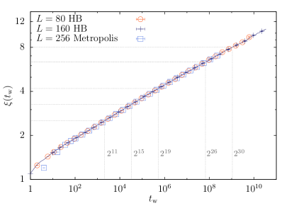
We have considered five different values of $t_{\mathrm{w}}$: $t_{\mathrm{w}}=2^{11}$ and $t_{\mathrm{w}}=2^{30}$ were simulated on Janus II; $t_{\mathrm{w}}=2^{26},2^{19}$ and $2^{15}$ on Janus (smaller systems were simulated on Memento, see below our study of size effects). Times are measured in units of Monte Carlo sweeps. The measuring times $t$ were chosen as the integer part of $2^{i/4}$ for integer $i$ (discarding repetitions). For each $t_{\mathrm{w}}$ we repeat the procedure described above for four values of the magnetic field: $H\in\{0,0.02,0.04,0.08\}$ in the case of Memento and Janus I supercomputers and $H\in\{0,0.01,0.02,0.04\}$ on Janus II. We considered exactly the same set of samples with each $H$ and reused the same sequences of random numbers in an effort to eliminate sources of fluctuations.

Depending on the computer used, we simulated different system sizes, either $L=80$ (on Memento and Janus I) or $L=160$ (on Janus II). We simulated 647 samples for $L=80$ (all $t_{\mathrm{w}}$ and $H$ values). For $L=160$, we used 55 samples for $t_{\mathrm{w}}=2^{11}$ and 335 samples for $t_{\mathrm{w}}=2^{30}$ [we also simulated 336 samples at $H=0$ in order to compute $\xi(t_{\mathrm{w}})$]. Notice that self-averaging means that one needs fewer samples for larger sizes. Previous works at $H=0$ suggested that finite-size effects should be negligible, compared to our typical statistical accuracy, as long as we ensure that $L>7\xi(t+t_{\mathrm{w}})$ Belletti et al. (2008a). As a new test of the validity of this statement, we compare our new results of $\xi(t_{\mathrm{w}})$ obtained with Janus II and $L=160$ with previous works corresponding to $L=80$ Belletti et al. (2009b) and $L=256$ Fernández and Martín-Mayor (2015) (see Fig. 6) finding no significant dependence on $L$ in the studied range of $t_{\mathrm{w}}$.

Appendix C Computation of the linear susceptibility

The discussion on the GFDR requires the computation of the linear susceptibility, that is, of

$$\chi(t+t_{\mathrm{w}},t_{\mathrm{w}})=\left.\frac{\partial m(t+t_{\mathrm{w}})}{\partial H}\right|_{H=0}.$$ (15)

With this aim, we measure $m(t,t_{\mathrm{w}})/H$ at several values of the external field, and use them to extract the $H\to 0$ limit. Indeed, since the Edwards-Anderson Hamiltonian is odd in the field around $H=0$, one can write the magnetization in terms of odd powers of $H$, which allows us to separate the linear response $\chi$ from the non-linear responses

$${m(t+t_{\mathrm{w}},t_{\mathrm{w}};H)}=H\chi(t+t_{\mathrm{w}},t_{\mathrm{w}})-\frac{H^{3}}{3!}\chi_{\mathrm{NL}}(t+t_{\mathrm{w}},t_{\mathrm{w}};H).$$ (16)

In order to make some progress, we Taylor-expand $\chi_{\mathrm{NL}}=\chi_{3}+\frac{H^{2}}{20}\chi_{5}+\mathcal{O}(H^{4})$, thus finding:

$$\begin{split}\frac{m(t+t_{\mathrm{w}},t_{\mathrm{w}})}{H}=&\chi(t+t_{\mathrm{w}},t_{\mathrm{w}})-\frac{H^{2}}{3!}\chi_{3}(t+t_{\mathrm{w}},t_{\mathrm{w}})\\ &\quad-\frac{H^{4}}{5!}\chi_{5}(t+t_{\mathrm{w}},t_{\mathrm{w}})+\mathcal{O}(H^{6}),\end{split}$$ (17)

Therefore, if we measure $m$ for three small fields and neglect higher-order contributions in $H$, we can extract $\chi(t+t_{\mathrm{w}},t_{\mathrm{w}})$ from a set of three equations and three unknowns [by the same token, we obtain $\chi_{3}(t+t_{\mathrm{w}},t_{\mathrm{w}})$ and $\chi_{5}(t+t_{\mathrm{w}},t_{\mathrm{w}})$ as well, but these magnitudes will not be discussed herein]. We show in Fig. 7 $m(t+t_{\mathrm{w}},t_{\mathrm{w}})/H$ and $\chi(t+t_{\mathrm{w}},t_{\mathrm{w}})$ for one of our values of $t_{\mathrm{w}}$.

Figure 7: Extraction of the linear susceptibility as a function of $t$ from the $m(t+t_{\mathrm{w}},t_{\mathrm{w}})/H$ data obtained at $H=0.02,\ 0.04$ and $0.08$. Data shown here corresponds to $t_{\mathrm{w}}=2^{26}$. For the sake of visibility, only one every two measured times have been plotted in points.

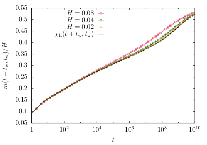
Alternatively, instead of performing simulations at different $H$, one could have obtained $\chi(t+t_{\mathrm{w}},t_{\mathrm{w}})$ directly from simulations at $H=0$ using methods such as those described in Refs. Ricci-Tersenghi (2003); Chatelain (2003). The drawback of this approach is that it would have required a much larger amount of samples in order to get equivalent statistical errors.

Appendix D Smoothing and interpolating the data

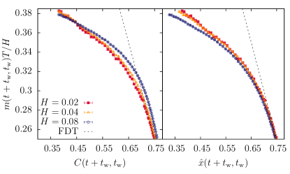
The original data consisted of pairs $\{C(t+t_{\mathrm{w}},t_{\mathrm{w}}),\chi(t+t_{\mathrm{w}},t_{\mathrm{w}})\}$, where $t$ takes some discrete values. However, if we reproduce Fig. 1 in the main text but using the raw measurements (see Fig. 8) we find much noisier curves. Indeed, data for successive times, although very correlated, displays random fluctuations. Besides, the statistical errors for $C(t+t_{\mathrm{w}},t_{\mathrm{w}};H=0)$ and $C(t+t_{\mathrm{w}},t_{\mathrm{w}};H)$ are completely negligible compared to the errors in $Tm(t+t_{\mathrm{w}},t_{\mathrm{w}};H)/H$ (they are indistinguishable in the figure). We used these two facts to our benefit in order to smooth and reduce the statistical errors of these curves. Let us describe our smoothing procedure step by step.

Figure 8: Linear response $T\chi(t,t_{\mathrm{w}})$ versus $C(t+t_{\mathrm{w}},t_{\mathrm{w}})$ at $T=0.7$ and five values of $t_{\mathrm{w}}$ using raw processed data (to be compared with Fig. 1 in the main text, which was obtained only after the smoothing of the simulation data at fixed $H$ and an extrapolation to $H\to 0$).

We fit our data for $Tm(t+t_{\mathrm{w}},t_{\mathrm{w}};H)/H$ to a smooth function of

$$\hat{x}(t+t_{\mathrm{w}},t_{\mathrm{w}})=\frac{C(t+t_{\mathrm{w}},t_{\mathrm{w}})+C(t+t_{\mathrm{w}},t_{\mathrm{w}};H)}{2}\,.$$ (18)

This choice [instead of just $C(t+t_{\mathrm{w}},t_{\mathrm{w}})$], although irrelevant in the $H\to 0$ limit, turns out to reduce the non-linear corrections in $H$ as we show in Fig. 9, and yields easier and more accurate fits.

Figure 9: Non-linear corrections in $H$ to $T\chi(t+t_{\mathrm{w}},t_{\mathrm{w}})$ when plotted versus $C(t+t_{\mathrm{w}},t_{\mathrm{w}})$ (left) or $x(t+t_{\mathrm{w}},t_{\mathrm{w}})=C(t+t_{\mathrm{w}},t_{\mathrm{w}})+C(t+t_{\mathrm{w}},t_{\mathrm{w}};H)/2$ (right). Data corresponds to $t_{\mathrm{w}}=2^{26}$ and $T=0.7$.

Our chosen functional form is as follows. Let the quantity $Tm(t+t_{\mathrm{w}},t_{\mathrm{w}};H)/H$ be approximated by $f(\hat{x})$ ($f$ depends on $H$ and $t_{\mathrm{w}}$, but we will write $f$ nevertheless, to keep the notation as light as possible):

$$f(\hat{x})=f_{\mathrm{L}}(\hat{x})\frac{1+\tanh[Q(\hat{x})]}{2}\,+\,f_{\mathrm{S}}(\hat{x})\frac{1-\tanh[Q(\hat{x})]}{2}\,,$$ (19)

with $Q(\hat{x})=(\hat{x}-\hat{x}^{*})/w$. In other words, there are two functional forms: $f_{\mathrm{S}}$, adequate for small $\hat{x}$ and $f_{\mathrm{L}}$, good for large $\hat{x}$. The crossover between the two functional forms takes place at $\hat{x}^{*}\approx 0.7$ in an interval of half-width $w\approx 0.04$ (although we keep $\hat{x}^{*}$ and $w$ as fitting parameters). The functional form for small $\hat{x}$ are diagonal [$N,N$] Padè approximants,

$$f_{\mathrm{S}}(\hat{x})=\frac{\sum_{k=0}^{N}b_{k}\hat{x}^{k}}{\sum_{k=0}^{N}a_{k}\hat{x}^{k}}\,.$$ (20)

As for the region where deviations from the fluctuation-dissipation theorem are tiny, we chose a polynomial in $1-\hat{x}$

$$f_{\mathrm{L}}(\hat{x})=(1-\hat{x})+\sum_{k=2}^{N^{\prime}}c_{k}(1-\hat{x})^{k}.$$ (21)

We keep ${a_{k},b_{k},c_{k}}$ as fitting variables.

Following Refs. Belletti et al. (2008a, 2009b); Fernández and Martín-Mayor (2015); Lulli et al. (2016), we perform a fit considering only the diagonal part of the covariance matrix (we obtain $\chi^{2}/\mathrm{DOF}$ significantly smaller than one, probably due to data correlation). Errors are computed following a jackknife procedure [we perform an independent fit for each jackknife block, and compute errors from the jackknife fluctuations of the fitted $f(\hat{x})$]. Our fits are reported in Table 1.

Table 1: Information about the fits to Eqs. (19,20,21).

$t_{\mathrm{w}}$	$H$	$N$	$N^{\prime}$	$\chi^{2}/\mathrm{DOF}$
	0.01	2	1	51.6822/127
$2^{11}$	0.02	2	1	43.9926/127
	0.04	2	1	45.6321/127
	0.02	2	1	33.1259/90
$2^{15}$	0.04	2	1	43.3823/90
	0.08	2	2	21.0832/89
	0.02	3	2	27.6364/115
$2^{19}$	0.04	3	2	25.8737/115
	0.08	3	3	31.6819/114
	0.02	2	1	29.5259/118
$2^{26}$	0.04	2	1	36.5544/118
	0.08	2	1	57.3693/118
	0.01	2	1	31.7369/126
$2^{30}$	0.02	3	3	24.7701/122
	0.04	3	2	33.0019/123

Once each curve $Tm(t+t_{\mathrm{w}},t_{\mathrm{w}})/H$ is smoothed at each $H$, we extract the linear susceptibility following the procedure described in the previous Section. We show a comparison between the original and smoothed data in Fig. 10. We found that in most the cases the extrapolated linear response $T\chi(t+t_{\mathrm{w}},t_{\mathrm{w}})$ was compatible within the error with the smaller field considered. However, the extrapolation $H\to 0$ becomes particularly delicate and even changes the shape of the curve at large values of the $t/t_{\mathrm{w}}$ ratio, as we show in Fig. 11.

Figure 10: Comparison between the original (in color and empty dots) and smoothed data (in black full dots) in the Linear response $T\chi(t+t_{\mathrm{w}},t_{\mathrm{w}})$ versus $C(t+t_{\mathrm{w}},t_{\mathrm{w}})$ curves. Data corresponds to $T=0.7$ and five values of $t_{\mathrm{w}}$.

Figure 11: $Tm(t+t_{\mathrm{w}},t_{\mathrm{w}})/H$ versus $\hat{x}(t+t_{\mathrm{w}},t_{\mathrm{w}})$ for several values of $H$ (in color empty dots) and $t_{\mathrm{w}}=2^{11}$, together with the extrapolation $H\to 0$ (in black crosses). The inset is a blow up of the region for large $t/t_{\mathrm{w}}$ in the square box.

Appendix E Fit of $S(C,L)$ and computation of $L_{\mathrm{eff}}$

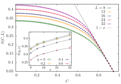
Part of our discussion in the main text seeks to find a relation between the linear response at finite $t_{\mathrm{w}}$ with the overlap distribution $P(q,L)$ in equilibrium at a finite size $L_{\mathrm{eff}}$. That is,

$$T\chi(t+t_{\mathrm{w}},t_{\mathrm{w}})=S\big{(}C(t+t_{\mathrm{w}},t_{\mathrm{w}}),L_{\mathrm{eff}}(t+t_{\mathrm{w}},t_{\mathrm{w}})\big{)}\,,$$ (22)

where

$$S(C,L)=\int_{C}^{1}d\mathrm{C^{\prime}}\,x(C^{\prime},L)\,,\ x(C,L)=\int_{0}^{C}\,\mathrm{d}q\,2P(q,L)\,.$$ (23)

We computed $S(C,L)$ by means of a numerical integration of the $P(q,L)$ discussed in Ref. Baños et al. (2010a) for $L=8,\ 12,\ 16,\ 24$ and $32$. We show $S(C,L)$ in the main panel of Fig. 12. In order to identify $L_{\mathrm{eff}}$ we needed a function $S(q,x)$ that is continuous both in $C$ and in $L$, which we construct by computing a cubic spline of the data along both variables (first in $C$ and only then in $L$). Errors are computed using the jackknife method. We show some interpolation curves along the $x$ variable in the inset of Fig. 12. Once $S(q,x)$ is at hand, $L_{\mathrm{eff}}(t+t_{\mathrm{w}},t_{\mathrm{w}})$ can be extracted by looking for the $x$ value that satisfies (22) at each time $t$, fixing the off-equilibrium data $T\chi(t+t_{\mathrm{w}},t_{\mathrm{w}})$ and $C(t,t_{\mathrm{w}})$.

Figure 12: $S(C,L)$ versus $C$ for different system sizes obtained using (14) and data from Ref. Baños et al. (2010a). (Inset) Orthogonal cuts to the figure in the main panel plotted as function of $L$ in color points together with the interpolating cubic spline curve along this variable.

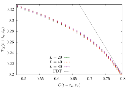
Appendix F Finite-size effects in the response

Up to now, finite-size effects have been investigated only for single-time correlation functions [and the related extraction of $\xi(t_{\mathrm{w}})$]. As far as we know, size effects were not studied previously in the response to a magnetic field $\chi(t+t_{\mathrm{w}},t_{\mathrm{w}})$. In this context, it is somewhat worrying that we have identified a large length scale $L_{\mathrm{eff}}\approx 100$ (discussed below) in the regime where deviations from the FDT are incipient. For this reason, we have explicitly checked that our data does not suffer from finite-size effects in that region (as we show in Fig. 13) by comparing results from three system sizes, $L=20,\ 40$ and $80$, in the case of $t_{\mathrm{w}}=2^{15}$, finding no finite-size dependence. For the smaller system sizes we considered 28000 samples for $L=20$ and 12000 samples for $L=40$.

Figure 13: Absence of finite-size effects in the response function $T\chi(t+t_{\mathrm{w}},t_{\mathrm{w}})$ versus $C(t+t_{\mathrm{w}},t_{\mathrm{w}})$ at $T=0.7$. Data from $L=20,\ 40$ and $80$ are compared in the case of $t_{\mathrm{w}}=2^{15}$. All the points are compatible within the error bars.

Appendix G A simple inequality

In the main text, we have used several times the inequality

$$S(C,L)\leq 1-\overline{\langle|q|\rangle}_{L=\infty}\,.$$ (24)

Our purpose here is to remind the reader of its derivation, for the sake of completeness.

Let us first recall the notations used in the main text:

$$S(C,L) = \int_{C}^{1}d\mathrm{C^{\prime}}\,x(C^{\prime},L)\,,$$ (25)

$$x(C,L) = \int_{0}^{C}\,\mathrm{d}q\,2P(q,L)\,.$$ (26)

We start by noticing

$$S(C,L)\leq S(C=0,L)\,,$$ (27)

due to the inequality $x(C,L)\geq 0$ for the cumulative distribution. Next, we integrate by parts to find [recall that $P(q,L)=P(-q,L)$]

$$S(C=0,L)=1-\overline{\langle|q|\rangle}_{L}\,,\quad\overline{\langle|q|\rangle}_{L}\equiv\int_{-1}^{1}\,\mathrm{d}q|q|P(q,L)\,.$$ (28)

Finally, to obtain the upper bound in (24), we remark that $\overline{\langle|q|\rangle}_{L}$ is monotonically decreasing in $L$ for a system with periodic boundary conditions.

Appendix H The ferromagnetic case and conditions for validity of Eq. (5) of main text

Figure 14: Upper lines with points are data for $T\chi(t+t_{\mathrm{w}},t_{\mathrm{w}})$ versus $C(t+t_{\mathrm{w}},t_{\mathrm{w}})$ measured in the $D=2$ ferromagnetic Ising model at $T=2\approx 0.88T_{c}$ (data from Ref. Ricci-Tersenghi (2003)). Lower lines are the equilibrium $S(C,L)$ for the same model and their thermodynamic limit $S(C,L=\infty)$. For this model Eq. (5) of main text can not be satisfied and the SDD does not exist.

Our SDD is based on Eq. (5) in the main text that we repeat here for readers convenience

$$T\chi(t+t_{\mathrm{w}},t_{\mathrm{w}})=S\big{(}C(t+t_{\mathrm{w}},t_{\mathrm{w}}),L_{\mathrm{eff}}(t+t_{\mathrm{w}},t_{\mathrm{w}})\big{)}\,.$$ (29)

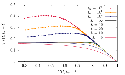
Although for the $D=3$ Edwards-Anderson (EA) model the above equation can be satisfied for all our data, it is not obvious that this is the case for other models. In particular we show in Fig. 14 a simple case where (29) can not be satisfied.

In Fig. 14 we show both equilibrium and non-equilibrium data for the $D=2$ ferromagnetic Ising model gathered at temperature $T=2\approx 0.88T_{c}$. For the non-equilibrium data we reproduce correlation and responses already published in Ref. Ricci-Tersenghi (2003), while the equilibrium data have been obtained by running the Wolff algorithm Wolff (1989). The black line is the thermodynamical limit for the equilibrium data

$$S(C,\infty)=\min(1-m(T)^{2},1-C)$$

where $m(T)$ is the remanent magnetization.

It is clear from data in Fig. 14 that there is no $L_{\mathrm{eff}}$ size such that the non-equilibrium data can be matched with the equilibrium ones. This is a direct consequence of the fact that finite size effects in this model are such that $S(C,L)\leq S(C,\infty)$, while the dynamical curves show an excess of response, bringing them above $S(C,\infty)$.

In general the condition for the applicability of (29) is that the dynamical curves must lie in the region of the $(T\chi,C)$ plane covered by the equilibrium functions $S(C,L)$. In the present case such a region is very narrow (as shown in Fig. 14 for $L\geq 5$) and the dynamical curves miss it. Luckily enough the analogous region for the $D=3$ EA model is very wide, and (29) can be always satisfied on the timescales we have probed.

The very different behaviour between the above two models can be explained by noticing that there are at least two major sources of finite times effects:

• the first is the one discussed thoroughly in the main text. Its application to the ferromagnetic Ising model should give a really tiny effect, because the $S(C,L)$ converges very fast to its thermodynamical limit;

• the second correction comes from the convergence of one-time quantities (e.g. the energy density) to their large time limit. This is the dominating one for the ferromagnetic Ising model, where the energy density decays as $E(t)-E(\infty)\propto\xi(t)^{-b}$, with $b=1$. We expect this contribution to be much less important in the EA model, since the exponent is $b\simeq 2.6$ Belletti et al. (2009b). The ferromagnetic Ising model is very peculiar; in the general case, using the hand-waiving argument that the exponent $b$ equals the lower critical dimension, we expect $b>1$ (e.g. $b=2$ in models with continuous variables) and this correction to be much less relevant.

Appendix I Extrapolating the effective size

We have shown in the main text that, for every $t_{\mathrm{w}}$ and small enough $t$, $L_{\mathrm{eff}}(t+t_{\mathrm{w}},t_{\mathrm{w}})$ can be very large. This short-time but large-size effect arises when $C(t+t_{\mathrm{w}},t\mathrm{w})\approx q_{\mathrm{EA}}^{L=4\xi(t_{\mathrm{w}})}$. In fact, for $t_{\mathrm{w}}=2^{30}$ (our largest) we can compute $L_{\mathrm{eff}}$ without extrapolations only for the largest $t$.

The above observation begs the question: how large can $L_{\mathrm{eff}}$ be in this small-$t$ regime? We provide here a crude extrapolation for our $t_{\mathrm{w}}=2^{30}$ data, mostly based on the scaling laws found in Baños et al. (2010a).

We start by noticing that one could be tempted to extract the spin-overlap probability directly from the aging response. One can define the dynamic overlap probability density function:

$$P_{\mathrm{dyn}}(q;t_{\mathrm{w}})=-\frac{1}{2}\left.\frac{\partial^{2}T\chi(C,t_{\mathrm{w}})}{\partial C^{2}}\right|_{C=q}\,.$$ (30)

Then, one could compare $P_{\mathrm{dyn}}$ with the equilibrium $P(q,L)$ at $q=C(t+t_{\mathrm{w}},t_{\mathrm{w}})$. The weak point in this approach is that taking two derivatives of the curve $T\chi(C,t_{\mathrm{w}})$, which is subject to random errors, is very difficult.

Our way out will be to recall that the area under the peak of the $P(q,L)$ is approximately $L$-independent Baños et al. (2010a). Therefore, we shall estimate the peak height (rather than the peak width).

Our efforts to locate the maximum (let alone the full curve) for $P_{\mathrm{dyn}}(q;t_{\mathrm{w}}=2^{30})$ are documented in Fig. 15 (but the reader is warned to take the results cum grano salis). We note from Fig. 15 that the ratio of the height of the maxima for $t_{\mathrm{w}}=2^{30}$ and $L=32$ is $\sim 3.6/2.5$. Therefore, from the scaling of the peak width, $\propto L^{-B\approx 0.28}$, we extrapolate

$$L_{\mathrm{eff}}\sim 32\times(3.6/2.5)^{\frac{1}{B}}\approx 118\,,$$ (31)

which is certainly larger than our maximum equilibrium size, $L=32$.

Figure 15: Numerical attempt to locate the maximum of $P_{\mathrm{dyn}}(q,t_{\mathrm{w}}=2^{30})$. In the top panel, we compare the dynamic response $T\chi(C,t_{\mathrm{w}}=2^{30})$ with the equilibrium curve $S(C,L=32)$. The range of $C$ covers the peak width of $P(q,L=32)$ Baños et al. (2010a). Since the curvature is clearly larger for $T\chi$ than for $S(C,L=32)$, (30) tells us that that the maximum of $P_{\mathrm{dyn}}(q;t_{\mathrm{w}}=2^{30})$ is higher than the maximum of $P(q,L=32)$. The lines correspond to diagonal fits to fourth order polynomials in $C$ (we increased the order of the polynomial until the figure of merit diagonal-$\chi^{2}$ for the fit of the dynamic response no longer decreased). The bottom panel shows the second derivative of the interpolating polynomials of the top panel, multiplied by $-1/2$. According to  (30), these derivatives should give us $P_{\mathrm{dyn}}(q,t_{\mathrm{w}})$ and $P(q,L)$. Indeed, the peak position and height in $P(q,L=32)$ is very reasonably reproduced by this approach, see Ref. Baños et al. (2010a).

Appendix J The simplified $S(C,L)$

In the main text, we wondered about the consequences of having at our disposal only a simplified approximation for $S(C,L)$:

$$S_{\mathrm{simpl}}(C,L)=\min\left[S_{0}(L)-P_{0}C^{2}-\frac{P_{1}}{6}C^{4},1-C\right]\,.$$ (32)

In the above equation, $P_{0}$ and $P_{1}$ are $L$-independent constants. All the depedence on the system size is in $S_{0}(L)$. In fact, $S_{0}(L)$ was obtained by fitting the actual data $S(C=0,L=8,12,16,24,32)$ to a quadratic polynomial in $L^{-\theta}$. We took $\theta=0.38$ from Ref. Baños et al. (2010a) [recall that the maximum of the spin-overlap probability, $P(q,L)$ scales with $L$ as $q_{\mathrm{EA}}^{(L)}-q_{\mathrm{EA}}^{(\infty)}\propto L^{-\theta}$]. Once $S_{0}(L)$ was known, we determined the constants $P_{0}$ and $P_{1}$ from a least-squares minimization of the difference between $S_{\mathrm{simpl}}(C,L)$ and the actual data.

References

- Cavagna (2009) A. Cavagna, Physics Reports 476, 51 (2009), arXiv:0903.4264 .
- Vincent et al. (1997) E. Vincent, J. Hammann, M. Ocio, J.-P. Bouchaud, and L. F. Cugliandolo, in Complex Behavior of Glassy Systems, Lecture Notes in Physics No. 492, edited by M. Rubí and C. Pérez-Vicente (Springer, 1997).
- Rodriguez et al. (2003) G. F. Rodriguez, G. G. Kenning, and R. Orbach, Phys. Rev. Lett. 91, 037203 (2003).
- Dupuis et al. (2005) V. Dupuis, F. Bert, J.-P. Bouchaud, J. Hammann, F. Ladieu, D. Parker, and E. Vincent, Pramana J. of Phys. 64, 1109 (2005).
- Barrat and Berthier (2001) A. Barrat and L. Berthier, Phys. Rev. Lett. 87, 087204 (2001).
- Belletti et al. (2008a) F. Belletti, M. Cotallo, A. Cruz, L. A. Fernandez, A. Gordillo-Guerrero, M. Guidetti, A. Maiorano, F. Mantovani, E. Marinari, V. Martín-Mayor, A. M. Sudupe, D. Navarro, G. Parisi, S. Perez-Gaviro, J. J. Ruiz-Lorenzo, S. F. Schifano, D. Sciretti, A. Tarancon, R. Tripiccione, J. L. Velasco, and D. Yllanes (Janus Collaboration), Phys. Rev. Lett. 101, 157201 (2008a), arXiv:0804.1471 .
- Baños et al. (2010a) R. A. Baños, A. Cruz, L. A. Fernandez, J. M. Gil-Narvion, A. Gordillo-Guerrero, M. Guidetti, A. Maiorano, F. Mantovani, E. Marinari, V. Martín-Mayor, J. Monforte-Garcia, A. Muñoz Sudupe, D. Navarro, G. Parisi, S. Perez-Gaviro, J. J. Ruiz-Lorenzo, S. F. Schifano, B. Seoane, A. Tarancon, R. Tripiccione, and D. Yllanes (Janus Collaboration), J. Stat. Mech. 2010, P06026 (2010a), arXiv:1003.2569 .
- Baños et al. (2010b) R. A. Baños, A. Cruz, L. A. Fernandez, J. M. Gil-Narvion, A. Gordillo-Guerrero, M. Guidetti, A. Maiorano, F. Mantovani, E. Marinari, V. Martín-Mayor, J. Monforte-Garcia, A. Muñoz Sudupe, D. Navarro, G. Parisi, S. Perez-Gaviro, J. J. Ruiz-Lorenzo, S. F. Schifano, B. Seoane, A. Tarancon, R. Tripiccione, and D. Yllanes (Janus Collaboration), Phys. Rev. Lett. 105, 177202 (2010b), arXiv:1003.2943 .
- Oukris and Israeloff (2010) H. Oukris and N. E. Israeloff, Nature Physics 06, 135 (2010).
- Komatsu et al. (2011) K. Komatsu, D. L’Hôte, S. Nakamae, V. Mosser, M. Konczykowski, E. Dubois, V. Dupuis, and R. Perzynski, Phys. Rev. Lett. 106, 150603 (2011), arXiv:1010.4012 .
- Cugliandolo and Kurchan (1993) L. F. Cugliandolo and J. Kurchan, Phys. Rev. Lett. 71, 173 (1993).
- Franz and Rieger (1995) S. Franz and H. Rieger, Journal of Statistical Physics 79, 749 (1995).
- Marinari et al. (1998) E. Marinari, G. Parisi, F. Ricci-Tersenghi, and J. J. Ruiz-Lorenzo, Journal of Physics A: Mathematical and General 31, 2611 (1998).
- Franz et al. (1998) S. Franz, M. Mézard, G. Parisi, and L. Peliti, Phys. Rev. Lett. 81, 1758 (1998).
- Franz et al. (1999) S. Franz, M. Mézard, G. Parisi, and L. Peliti, Journal of Statistical Physics 97, 459 (1999).
- Marinari et al. (2000a) E. Marinari, G. Parisi, F. Ricci-Tersenghi, and J. J. Ruiz-Lorenzo, J. Phys. A 33, 2373 (2000a).
- Hérisson and Ocio (2002) D. Hérisson and M. Ocio, Phys. Rev. Lett. 88, 257202 (2002), arXiv:cond-mat/0112378 .
- Cruz et al. (2003) A. Cruz, L. A. Fernández, S. Jiménez, J. J. Ruiz-Lorenzo, and A. Tarancón, Phys. Rev. B 67, 214425 (2003).
- Hérisson and Ocio (2004) D. Hérisson and M. Ocio, Eur. Phys. J. B 40, 283 (2004), arXiv:cond-mat/0403112 .
- Parisi (1979) G. Parisi, Phys. Rev. Lett. 43, 1754 (1979).
- Kawamura (2003) H. Kawamura, Phys. Rev. Lett. 90, 237201 (2003).
- Billoni et al. (2005) O. V. Billoni, S. A. Cannas, and F. A. Tamarit, Phys. Rev. B 72, 104407 (2005).
- Parisi (1997) G. Parisi, Phys. Rev. Lett. 79, 3660 (1997).
- Barrat and Kob (1999) J.-L. Barrat and W. Kob, EPL (Europhysics Letters) 46, 637 (1999).
- Barrat and Berthier (2000) J.-L. Barrat and L. Berthier, Phys. Rev. E 63, 012503 (2000).
- Berthier (2007) L. Berthier, Phys. Rev. Lett. 98, 220601 (2007).
- Gnan et al. (2013) N. Gnan, C. Maggi, G. Parisi, and F. Sciortino, Phys. Rev. Lett. 110, 035701 (2013).
- Grigera and Israeloff (1999) T. S. Grigera and N. E. Israeloff, Phys. Rev. Lett. 83, 5038 (1999).
- Bellon et al. (2001) L. Bellon, S. Ciliberto, and C. Laroche, EPL (Europhysics Letters) 53, 511 (2001).
- Maggi et al. (2010) C. Maggi, R. Di Leonardo, J. C. Dyre, and G. Ruocco, Phys. Rev. B 81, 104201 (2010).
- Maggi et al. (2012) C. Maggi, R. Di Leonardo, G. Ruocco, and J. C. Dyre, Phys. Rev. Lett. 109, 097401 (2012).
- Gomez-Solano et al. (2009) J. R. Gomez-Solano, A. Petrosyan, S. Ciliberto, R. Chetrite, and K. Gawędzki, Phys. Rev. Lett. 103, 040601 (2009).
- Jop et al. (2009) P. Jop, J. R. Gomez-Solano, A. Petrosyan, and S. Ciliberto, Journal of Statistical Mechanics: Theory and Experiment 2009, P04012 (2009).
- Greinert et al. (2006) N. Greinert, T. Wood, and P. Bartlett, Phys. Rev. Lett. 97, 265702 (2006).
- Bonn and Kegel (2003) D. Bonn and W. K. Kegel, The Journal of Chemical Physics 118, 2005 (2003).
- Dieterich et al. (2015) E. Dieterich, J. Camunas-Soler, M. Ribezzi-Crivellari, U. Seifert, and F. Ritort, Nat Phys 11, 971 (2015).
- Belletti et al. (2008b) F. Belletti, M. Cotallo, A. Cruz, L. A. Fernandez, A. Gordillo, A. Maiorano, F. Mantovani, E. Marinari, V. Martín-Mayor, A. Muñoz Sudupe, D. Navarro, S. Perez-Gaviro, J. J. Ruiz-Lorenzo, S. F. Schifano, D. Sciretti, A. Tarancon, R. Tripiccione, and J. L. Velasco (Janus Collaboration), Comp. Phys. Comm. 178, 208 (2008b), arXiv:0704.3573 .
- Baity-Jesi et al. (2014) M. Baity-Jesi, R. A. Baños, A. Cruz, L. A. Fernandez, J. M. Gil-Narvion, A. Gordillo-Guerrero, D. Iniguez, A. Maiorano, F. Mantovani, E. Marinari, V. Martín-Mayor, J. Monforte-Garcia, A. Muñoz Sudupe, D. Navarro, G. Parisi, S. Perez-Gaviro, M. Pivanti, F. Ricci-Tersenghi, J. J. Ruiz-Lorenzo, S. F. Schifano, B. Seoane, A. Tarancon, R. Tripiccione, and D. Yllanes (Janus Collaboration), Comp. Phys. Comm 185, 550 (2014), arXiv:1310.1032 .
- Gunnarsson et al. (1991) K. Gunnarsson, P. Svedlindh, P. Nordblad, L. Lundgren, H. Aruga, and A. Ito, Phys. Rev. B 43, 8199 (1991).
- Palassini and Caracciolo (1999) M. Palassini and S. Caracciolo, Phys. Rev. Lett. 82, 5128 (1999), arXiv:cond-mat/9904246 .
- Ballesteros et al. (2000) H. G. Ballesteros, A. Cruz, L. A. Fernandez, V. Martín-Mayor, J. Pech, J. J. Ruiz-Lorenzo, A. Tarancon, P. Tellez, C. L. Ullod, and C. Ungil, Phys. Rev. B 62, 14237 (2000), arXiv:cond-mat/0006211 .
- Joh et al. (1999) Y. G. Joh, R. Orbach, G. G. Wood, J. Hammann, and E. Vincent, Phys. Rev. Lett. 82, 438 (1999).
- Bert et al. (2004) F. Bert, V. Dupuis, E. Vincent, J. Hammann, and J.-P. Bouchaud, Phys. Rev. Lett. 92, 167203 (2004).
- Berthier et al. (2005) L. Berthier, G. Biroli, J.-P. Bouchaud, L. Cipelletti, D. El Masri, D. L’Hôte, F. Ladieu, and M. Pierno, Science 310, 1797 (2005).
- Young (1998) A. P. Young, Spin Glasses and Random Fields (World Scientific, Singapore, 1998).
- Cruz et al. (2001) A. Cruz, J. Pech, A. Tarancon, P. Tellez, C. L. Ullod, and C. Ungil, Comp. Phys. Comm 133, 165 (2001), arXiv:cond-mat/0004080 .
- Ogielski (1985) A. T. Ogielski, Phys. Rev. B 32, 7384 (1985).
- Belletti et al. (2009a) F. Belletti, M. Guidetti, A. Maiorano, F. Mantovani, S. F. Schifano, R. Tripiccione, M. Cotallo, S. Perez-Gaviro, D. Sciretti, J. L. Velasco, A. Cruz, D. Navarro, A. Tarancon, L. A. Fernandez, V. Martín-Mayor, A. Muñoz-Sudupe, D. Yllanes, A. Gordillo-Guerrero, J. J. Ruiz-Lorenzo, E. Marinari, G. Parisi, M. Rossi, and G. Zanier (Janus Collaboration), Computing in Science and Engineering 11, 48 (2009a).
- Belletti et al. (2009b) F. Belletti, A. Cruz, L. A. Fernandez, A. Gordillo-Guerrero, M. Guidetti, A. Maiorano, F. Mantovani, E. Marinari, V. Martín-Mayor, J. Monforte, A. Muñoz Sudupe, D. Navarro, G. Parisi, S. Perez-Gaviro, J. J. Ruiz-Lorenzo, S. F. Schifano, D. Sciretti, A. Tarancon, R. Tripiccione, and D. Yllanes (Janus Collaboration), J. Stat. Phys. 135, 1121 (2009b), arXiv:0811.2864 .
- Note (1) In fact, the correlation functions decay exponentially with distance. Therefore, with periodic boundary conditions, size effects should decay exponentially with . Indeed, an explicit computation shows that, to our accuracy level, size corrections are completely negligible when Belletti et al. (2008a).
- Parisi et al. (1999) G. Parisi, F. Ricci-Tersenghi, and J. J. Ruiz-Lorenzo, Eur. Phys. J. 11, 317 (1999), arXiv:cond-mat/9811374 .
- Ricci-Tersenghi (2003) F. Ricci-Tersenghi, Phys. Rev. E 68, 065104 (2003).
- Fernández and Martín-Mayor (2015) L. A. Fernández and V. Martín-Mayor, Phys. Rev. B 91, 174202 (2015).
- Manssen et al. (2015) M. Manssen, A. K. Hartmann, and A. P. Young, Phys. Rev. B 91, 104430 (2015), arXiv:1501.06760 .
- Wittmann and Young (2016) M. Wittmann and A. P. Young, Journal of Statistical Mechanics: Theory and Experiment 2016, 013301 (2016).
- Mézard et al. (1987) M. Mézard, G. Parisi, and M. Virasoro, Spin-Glass Theory and Beyond (World Scientific, Singapore, 1987).
- Note (2) The reader will note that data for are slightly off, in Fig. 3. We attribute the effect to a strong statistical fluctuation, enhanced by the fact that all data points with the same are extremely correlated.
- Note (3) Note that the delta peak in (10\@@italiccorr) is a reasonable expectation only for an infinite system (see Methods).
- Marinari et al. (2000b) E. Marinari, G. Parisi, F. Ricci-Tersenghi, J. J. Ruiz-Lorenzo, and F. Zuliani, J. Stat. Phys. 98, 973 (2000b), arXiv:cond-mat/9906076 .
- Note (4) See Ref. Joh et al. (1996) for an experimental attempt to measure Parisi’s functional order parameter, unrelated to GFDR.
- Jaubert et al. (2007) L. C. Jaubert, C. Chamon, L. F. Cugliandolo, and M. Picco, J. Stat. Mech. 2007, P05001 (2007).
- Chamon and Cugliandolo (2007) C. Chamon and L. F. Cugliandolo, J. Stat. Mech. 2007, P07022 (2007).
- Lulli et al. (2016) M. Lulli, G. Parisi, and A. Pelissetto, Phys. Rev. E 93, 032126 (2016).
- Baity-Jesi et al. (2013) M. Baity-Jesi, R. A. Baños, A. Cruz, L. A. Fernandez, J. M. Gil-Narvion, A. Gordillo-Guerrero, D. Iniguez, A. Maiorano, F. Mantovani, E. Marinari, V. Martín-Mayor, J. Monforte-Garcia, A. Muñoz Sudupe, D. Navarro, G. Parisi, S. Perez-Gaviro, M. Pivanti, F. Ricci-Tersenghi, J. J. Ruiz-Lorenzo, S. F. Schifano, B. Seoane, A. Tarancon, R. Tripiccione, and D. Yllanes (Janus Collaboration), Phys. Rev. B 88, 224416 (2013), arXiv:1310.2910 .
- Mydosh (1993) J. A. Mydosh, Spin Glasses: an Experimental Introduction (Taylor and Francis, London, 1993).
- Chatelain (2003) C. Chatelain, Journal of Physics A: Mathematical and General 36, 10739 (2003).
- Note (5) We do not used the so-called “natural” cubic spline. Instead, we fixed the first and last derivative of the interpolating function from three points of a parabolic fit.
- Wolff (1989) U. Wolff, Phys. Rev. Lett. 62, 361 (1989).
- Joh et al. (1996) Y. G. Joh, R. Orbach, and J. Hammann, Phys. Rev. Lett. 77, 4648 (1996).