Convex Histogram-Based Joint Image Segmentation
with Regularized Optimal Transport Cost

Abstract

We investigate in this work a versatile convex framework for multiple image segmentation, relying on the regularized optimal mass transport theory. In this setting, several transport cost functions are considered and used to match statistical distributions of features. In practice, global multidimensional histograms are estimated from the segmented image regions, and are compared to referring models that are either fixed histograms given a priori, or directly inferred in the non-supervised case. The different convex problems studied are solved efficiently using primal-dual algorithms. The proposed approach is generic and enables multi-phase segmentation as well as co-segmentation of multiple images.

1 Introduction

Optimal transport in imaging

Optimal transport theory has received a lot of attention during the last decade as it provides a powerful framework to address problems which embed statistical constraints. In contrast to most distances from information theory (e.g. the Kullback-Leibler divergence), optimal transport takes into account the spatial location of the density mode and define robust distances between empirical distributions. The geometric nature of optimal transport, as well as the ability to compute optimal displacements between densities through the corresponding transport map, make this theory progressively mainstream in several applicative fields. In image processing, the warping provided by the optimal transport has been used for video restoration (Delon-midway, ), color transfer (Pitie07, ), texture synthesis (Jungpeyre_wassestein11, ), optical nanoscopy (brune20104d, ) and medical imaging registration (AHT04, ). It has also been applied to interpolation in computer graphics (Bonneel-displacement, ; 2015-solomon-siggraph, ) and surface reconstruction in computational geometry (digne-reconstruction, ).

The optimal transport distance has also been successfully used in various image processing and machine learning tasks, image retrieval (Rubner2000, ; Pele-ICCV, ), image segmentation (bresson_wasserstein09, ), image decomposition (TV_Kantorovich_SIAM14, ) or texture synthesis (Rabin_mixing_SSVM11, ).

Some limitations have been also shown and partially addressed, such as time complexity (Cuturi13, ; Bonneel_radon15, ; Schmitzer_jmiv16, ), regularization and relaxation of the transport map (Ferradans_siims14, ) for imaging purposes.

Image segmentation

Image segmentation has been the subject of active research for more than 20 years (see e.g. (Aubert_Kornprobst02, ; Cremers07, ) and references therein). For instance, we can refer to the seminal work of Mumford and Shah (Mumford_Shah89, ), or to its very popular approximation with level sets developed by Chan and Vese in (Chan_Vese01, ). This last work provides a very flexible algorithm to segment an image into two homogeneous regions, each one being characterized by its mean gray level value.

In the case of textured images, a lot of extensions of (Chan_Vese01, ) have been proposed to enhance the mean value image segmentation model by considering other kind of local information. For instance, local histograms are used in (Zhu95, ; bresson_wasserstein09, ), Gabor filters in (Chan_Vese02, ), wavelet packets in (Aujol03, ) and textures are characterized thanks to the structure tensor in (Brox03, ; Rousson03, ).

Advanced statistical based image segmentation models using first parametric models (such as the mean and variance), and then empirical distributions combined with adapted statistical distances such as the Kullback-Leibler divergence, have been thoroughly studied in the literature. One can for instance refer to the works in (Aubert02, ; Kim05, ; Brox06, ; Herbulot06, ) that consider the global histograms of the regions to segment and are also based on the Chan and Vese model (Chan_Vese01, ). It is important to notice that this class of approaches involves complex shape gradient computations for the level set evolution equation. Moreover, as these methods all rely on the evolution of a level set function (Osher88, ), it leads to non-convex methods that are sensitive to the initialization choice and only a local minimizer of the associated energy is computed.

Recently, convexification methods have been proposed to tackle this problem, as in (Chambolle042, ; Nikolova06, ; CD08, ; Berkels09, ; Pock10, ; Chambolle11, ; Brown11, ; Yildi12, ). The original Chan and Vese model (Chan_Vese01, ) can indeed be convexified, and a global solution can be efficiently computed, for instance with a primal-dual algorithm. By means of the coarea formula, a simple thresholding of this global solution provides a global minimizer of the original non-convex problem. The multiphase segmentation model based on level sets (Chan_Vese02, ) can also be treated with convexification methods. However, the thresholding of the estimated global minima does not anymore ensure to recover a global optimal multiphase segmentation (Pock09, ). Notice that such approaches have not been developed yet for global histogram segmentation with length boundary regularization.

Other models as in (rother2006, ; vicente2009joint, ; ayed2010graph, ; gorelick2012segmentation, ; Yuan12, ) use graph-based methods and max-flow formulations (punithakumar2012convex, ) in order to obtain good minima without level-set representation. Nevertheless, these approaches are restricted to bin-to-bin distances (for instance $\ell_{1}$ (rother2006, ), Bhattacharyya (Yuan12, ), $\ell_{2}$ (TVL2_segmentation, ) or $\chi^{2}$ (object_cosegmentation, )) between features’ histograms that are not robust enough to deal with non-uniform quantification or data outliers.

Optimal Transport and image segmentation

The use of Optimal Transport for image segmentation has been first investigated in (bresson_wasserstein09, ) for comparing local $1D$ histograms. In (PeyreWassersteinSeg12, ; mendoza, ), active contours approaches using the Wasserstein distance for comparing global multi-dimensional histograms of the region of interest have been proposed. Again, these non-convex active contours methods are sensitive to the initial contour. Moreover, their computational cost is very large, even if they include some approximations of the Wasserstein distance as in (PeyreWassersteinSeg12, ).

In order to deal with global distance between histograms while being independent of any initialization choice, convex formulations have been designed (papa_aujol, ; Swoboda13, ). In (papa_aujol, ), a $\ell_{1}$ norm between cumulative histograms is considered and gives rise to a fast algorithm. This is related to optimal transport only for 1D histograms of grayscale images. The authors of (Swoboda13, ) proposed to rely on the Wasserstein distance. In order to be able to optimize the corresponding functional, it requires to make use of sub-iterations to compute the proximity operator of the Wasserstein distance, which use is restricted to low dimensional histograms. Hence, we considered in (Rabin_ssvm15, ) a fast and convex approach involving regularization of the optimal transport distance through the entropic regularization of (Cuturi13, ). In this paper we investigate in detail this regularized model and look at its extension to multi-phase segmentation.

Co-segmentation

As already proposed in (Swoboda13, ), the studied convex framework can be extended to deal with the unsupervised co-segmentation of two images. The problem of co-segmentation (Vicente_co-seg_eccv10, ) consists in segmenting simultaneously multiple images that contain the same object of interest without any prior information. When the proportion between the size of the object and the size of the image is the same in all images, the model of (Swoboda13, ) can be applied. It aims at finding regions in different images having similar color distributions. However, this model is not suited for cases where the scale of the object vary. In the literature, state-of-the art approaches rely on graph representation. They are able to deal with small scale changes (Rubio, ) or large ones by considering global information on image subregions (Hochbaum, ) pre-computed with dedicated algorithms. Notice that convex optimization algorithms involving partial duality of the objective functional have been used for co-segmentation based on local features (Joulin, ). Such approach is able to deal with scale change of objects but it relies on high dimensional problems scale with $O(N^{2})$, where $N$ is the total number of pixels.

The use of robust optimal transport distances within a low dimensional formulation for the global co-segmentation of objects of different scales is thus an open problem that is addressed in this paper.

Contributions

The global segmentation models presented in this paper are based on the convex formulation for two-phase image segmentation of (papa_aujol, ) involving $\ell_{1}$ distances between histograms. Following (Swoboda13, ; Rabin_ssvm15, ), we consider the use of Wasserstein distance for global segmentation purposes. As in (Rabin_ssvm15, ), we rely on the entropic regularization (Cuturi13, ; CuturiDoucet14, ) of optimal transport distances in order to deal with accurate discretizations of histograms. Hence, this paper shares some common features with the recent work of (CuturiPeyre_smoothdualwasserstein, ) in which the authors investigate the use of the Legendre-Fenchel transform of regularized transport cost for imaging problems.

With respect to the preliminary version of this work presented in a conference (Rabin_ssvm15, ), the contributions of this paper are the following:

• we give detailed proofs of the computation of the functions and operators involved by the entropic regularization of optimal transport between non-normalized histograms.

• we generalize the framework to the case of multi-phase segmentation in order to find a partition of the images with respect to several priors;

• we provide numerous experiments exhibiting the properties of our framework;

• we extend our model to the co-segmentation of multiple images. Two convex models are proposed. The first one is able to co-segment an object with constant size in two images for general ground costs. The second one can deal with different scales of a common object contained in different images for a specific ground cost.

This paper is also closely related to the framework proposed in (Swoboda13, ). With respect to this method, our contributions are:

• the use of regularized optimal transport distances for dealing with high dimensional histograms;

• the generalization of the framework to multi-phase segmentation;

• the definition of co-segmentation model for more than $2$ images dealing with scale changes of objects.

2 Convex histogram-based image segmentation

2.1 Notation and definitions

We consider here vector spaces equipped with the Euclidean inner product $\langle.\,,\,.\rangle$ and the $\ell_{2}$ norm $\lVert.\rVert=\sqrt{\langle.\,,\,.\rangle}$. The conjugate linear operator of $A$ is denoted by $A^{*}$ and satisfies $\langle A.,.\rangle=\langle.,A^{*}.\rangle$. We denote as $\mathbf{1}_{n}\text{ and }\mathbf{0}_{n}\in\mathbb{R}^{n}$ the $n$-dimensional vectors filled with ones and zeros respectively, $x^{\mathsf{T}}$ the transpose of $x$, while Id stands for the identity operator. The concatenation of the vectors $x$ and $y$ into a vector is denoted $(x;y)$. Operations and functions on vectors and matrices are meant component-wise, such as inequalities:

$$X\leq Y\quad\Leftrightarrow\quad X_{ij}\leq Y_{ij}\quad\forall\,i,j$$

or exponential and logarithm functions:

$$\left(\exp X\right)({i,j})=\exp X_{i,j}\qquad\log X=\left(\log X_{i,j}\right)_{i,j}.$$

We refer to $\ell_{p}$ norm as ${\lVert x\rVert}_{p}=\left(\sum_{i}{\lvert x_{i}\rvert}^{p}\right)^{\frac{1}{p}}$. The norm of a linear operator $A$ is ${\lVert A\rVert}=\sup_{\lVert x\rVert=1}{\lVert Ax\rVert}$.

The operator $\operatorname{diag}(x)$ defines a square matrix whose diagonal is the vector $x$. The identity matrix is $\mathrm{Id}_{n}=\operatorname{diag}(\mathbf{1}_{n})$. The functions $\mathbbm{1}_{S}$ and $\chi_{S}$ are respectively the indicator and characteristic functions of a set $S$

$$\begin{split}\mathbbm{1}_{S}(x)=\begin{cases}1&\text{ if }x\in S\\ 0&\text{ otherwise }\end{cases}\!\!,\;\chi_{S}(x)=\begin{cases}0&\text{ if }x\in S\\ \infty&\text{ otherwise }\end{cases}.\end{split}$$

The Kronecker $\delta$ symbol is $\delta_{i,j}=1$ if $i=j$, and $\delta_{i,j}=0$ otherwise.

A histogram with $n$ bins is a vector $h\in\mathbb{R}^{n}_{+}$ with non-negative entries. The set

$${\cal S}_{m,n}:=\{x\in\mathbb{R}^{n}_{+},\langle x,\,\mathbf{1}_{n}\rangle=m\}$$ (1)

is the simplex of histogram vectors of total mass $m$ (${\cal S}_{1,n}$ being the $n$-dimensional probability simplex).

The operators $\operatorname{Prox}$ and Proj stand respectively for the Euclidean proximity and projection operators:

$$\begin{split}\operatorname{Prox}_{f}(x)&=\operatorname{argmin}_{y}\tfrac{1}{2}|\!|y-x|\!|^{2}+f(x)\\ {\text{Proj}}_{S}(x)&=\operatorname{argmin}_{y\in S}|\!|y-x|\!|=\operatorname{Prox}_{\;\chi_{S}}(x)\;.\end{split}$$

Functions $f$ for which the proximity operator is known in closed form, or at least that can be evaluated at a given point explicitly, are usually referred to as simple.

The Legendre-Fenchel conjugate $f^{*}$ of a lower semicontinuous convex function $f$ writes $f^{*}(y)=\sup_{x}\langle x,\,y\rangle-f(x)$, and satisfies the equality: $f^{**}=f$.

2.2 General formulation of distribution-based image segmentation

For sake of simplicity, we first describe the binary segmentation problem. The following framework can be extended to multi-phase segmentation, as lately shown in Section 2.4.

Let $I:x\in\Omega\mapsto I(x)\in\mathbb{R}^{d}$ be a multi-dimensional image, defined over the $N$-pixel domain $\Omega$ ($N=\lvert\Omega\rvert$), and ${\cal F}$ a feature-transform into $n$-dimensional descriptors: ${\cal F}I(x)\in\mathbb{R}^{n}$. The border of the domain is denoted $\partial\Omega$. We would like to define a binary segmentation $u:\Omega\mapsto\{0,1\}$ of the whole image domain, using two fixed probability distributions of features $a$ and $b$. Following the variational model introduced in (papa_aujol, ), we consider the energy

$$E(u)=\rho\mathop{{TV}}(u)+{S}(a,h(u))+{S}(b,h(\mathbf{1}-u))$$ (2)

where $\rho\geq 0$ is the regularization parameter, and

• the fidelity terms are defined using ${{S}}(.,.)$, a dissimilarity measure between distributions of features;

• $h(u)$ is the empirical discrete probability distribution of features ${\cal F}I$ using the binary map $u$, which is written as a sum of Dirac masses

  $$\!\!h(u):y\in\mathbb{R}^{n}\mapsto\frac{1}{\sum_{x\in\Omega}u(x)}\sum_{x\in\Omega}u(x)\delta_{{\cal F}I(x)}(y)\,;$$ (3)

• $\mathop{{TV}}(u)$ is the total variation norm of the binary image $u$, which is related to the perimeter of the region $R_{1}(u):=\{x\in\Omega\,|\,u(x)=1\}$ by the co-area formula.

Observe that this energy is highly non-convex, $h$ being a non linear operator, and that we would like to find a minimum $u^{\star}\in\{0,1\}^{N}$ over a non-convex set.

2.3 Convex relaxation of histogram-based segmentation energy

The authors of (papa_aujol, ) propose some relaxations and a reformulation in order to handle the minimization of energy (2) using convex optimization tools.

2.3.1 Probability map

First, it consists in considering solutions from the convex enveloppe of the binary set, i.e. using a segmentation variable $u:\Omega\mapsto[0,1]$ which can be interpreted as a weight function (probability map). A threshold is therefore required to obtain a binary segmentation of the image into the region corresponding to the prior distribution $a$

$$R_{t}(u):=\{x\in\Omega\,|\,u(x)\geq t\},$$ (4)

its complement $R_{t}(u)^{c}$ corresponding to prior distribution $b$. Other post-processing partition techniques may be considered and are discussed later.

It is worth mentioning that for the specific $\mathop{{TV}}$-$\ell_{1}$ approach of (Nikolova06, ), where the dissimilarity measure ${S}(u,u_{0})=|\!|u-u_{0}|\!|_{1}$ is the $\ell_{1}$ distance between the segmentation variable $u$ and a given prior binary segmentation variable $u_{0}$, such a relaxation still guaranties to find a global solution for the non-convex problem. However, there is no such a property in our general setting.

2.3.2 Feature histogram

Considering the continuous domain of the feature space, as done for instance in (PeyreWassersteinSeg12, ), may become numerically intractable for high dimensional descriptors. We consider instead histograms, as already proposed in (bresson_wasserstein09, ; papa_aujol, ).

The feature histogram of the probability map is denoted $H_{\cal X}(u)$ and defined as the quantized, non-normalized, and weighted histogram of the feature image ${\cal F}I$ using the relaxed variable $u:\Omega\mapsto[0,1]$ and a feature set ${\cal X}=\{X_{i}\in\mathbb{R}^{n}\}_{1\leq i\leq M_{X}}$ composed of $M_{X}$ bins indexed by $i\in\{1,\ldots M_{X}\}$

$$\left(H_{\cal X}(u)\right)_{i}=\sum_{x\in\Omega}u(x)\mathbbm{1}_{{\cal C}_{\cal X}(i)}({\cal F}I(x)),$$ (5)

where $X_{i}$ is the centroid of the corresponding bin $i$, and ${\cal C}_{\cal X}(i)\subset\mathbb{R}^{n}$ is the corresponding set of features (e.g. the Voronoï cell obtained from nearest-neighbor assignment). We can write $H_{\cal X}$ as a linear operator

$$H_{\cal X}:u\in\mathbb{R}^{N}\mapsto H_{\cal X}\cdot u\in\mathbb{R}^{M_{X}},$$ (6)

with matrix notation $H(i,x):=1$ if ${\cal F}I(x)\in{\cal C}_{\cal X}(i)$ and $0$ otherwise. Note that $H_{\cal X}\in\mathbb{R}^{M_{X}\times N}$ is a fixed hard assignment matrix that indicates which pixels of ${\cal F}I$ contribute to each bin of the histogram. As a consequence, we have the property

$$\langle H_{\cal X}\,u,\,\mathbf{1}_{N}\rangle=\sum_{x\in\Omega}u(x)=\langle u,\,\mathbf{1}_{N}\rangle,$$ (7)

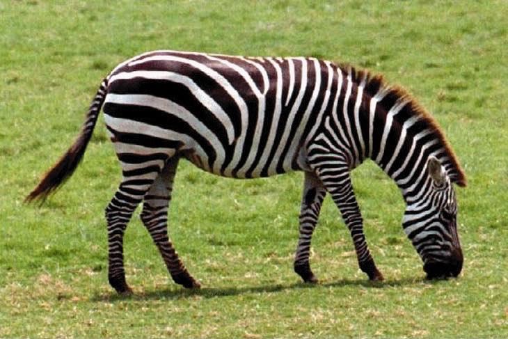
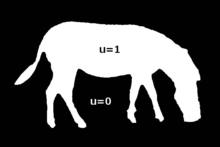
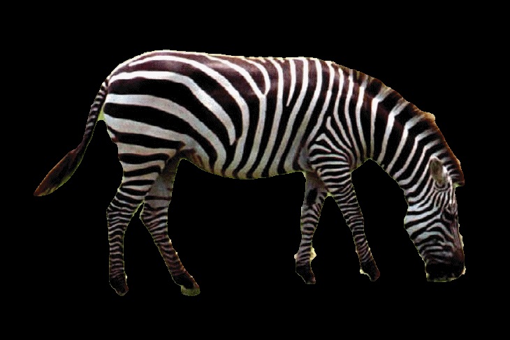
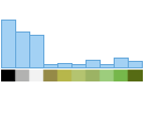
so that $H_{\cal X}(u)\in{\cal S}_{\langle u,\,\mathbf{1}\rangle,M_{X}}$. This linear operator computing the histogram of a particular region of the image is illustrated in Figure 1 for RGB color feature.

(a) Image $I$	(b) Segmentation $u$	(c) Region $I\odot u$

$\underbrace{\begin{bmatrix}1&0&0&1&\cdots&0\\ 0&1&0&0&\cdots&1\\ &&&\vdots\\ 0&0&0&0&\cdots&0\\ 0&0&1&0&\cdots&0\end{bmatrix}}_{H_{\cal X}}\times\underbrace{\begin{bmatrix}{0}\\ {1}\\ \vdots\\ {1}\\ {0}\end{bmatrix}}_{{u}}=\underbrace{\begin{bmatrix}n_{1}\\ n_{2}\\ \vdots\\ n_{M-1}\\ n_{M}\end{bmatrix}}_{H_{\cal X}\,u}=$

Figure 1: Illustration of the color histogram computed from a binary region. (a) Image $I$. (b) Binary segmentation map $u$. (c) Corresponding region $I\odot u(x)=I(x).u(x)$. The hard assignment linear operator $H_{\cal X}$ encodes the position of each pixel in the clustered color space. The histogram value $n_{i}$ represents here the number of pixels $I(x)$ of the region characterized by $u(x)=1$ that belongs to the feature cluster $C_{\cal X}(i)$.

2.3.3 Exemplar histograms

The segmentation is driven by two fixed histograms $a\in{\cal S}_{1,M_{a}}$ and $b\in{\cal S}_{1,M_{b}}$, which are normalized (i.e. sum to $1$), have respective dimension $M_{a}$ and $M_{b}$, and are obtained using the respective sets of features ${\cal A}$ and ${\cal B}$. In order to measure the similarity between the non-normalized histogram $H_{\cal A}(u)$ and the normalized histogram $a$, while obtaining a convex formulation, we follow (papa_aujol, ) and consider ${{S}}\left({a\langle u,\,\mathbf{1}_{N}\rangle,H_{\cal A}(u)}\right)$ as fidelity term, where the constant vector $a$ has been scaled to $H_{\cal A}(u)\in{\cal S}_{\langle u,\,\mathbf{1}\rangle,M_{a}}$.

Note that this approach, based on the comparison of unnormalized histogram pairs as a data fidelity term, is also used in (coseg_hist_matching, ; coseg_hist_matching_L2, ) for co-segmentation. We will further discuss the consequence of such a choice for this problem in the dedicated Section 6.

2.3.4 Segmentation energy

Using the previous modifications to formulation (2), the convex segmentation problem can now be written as finding the minimum of the following energy

$$\begin{split}J(u)&=\rho\mathop{{TV}}(u)+\tfrac{1}{\gamma}\,S\left({a\langle u,\,\mathbf{1}_{N}\rangle,H_{\cal A}u}\right)\\ &\hskip 34.1433pt+\tfrac{1}{N-\gamma}\,S\left({b\langle\mathbf{1}_{N}-u,\,\mathbf{1}_{N}\rangle,H_{\cal B}(\mathbf{1}_{N}-u)}\right).\end{split}$$

The constant $\gamma\in(0,N)$ is meant to compensate for the fact that the binary regions $R_{t}(u)$ and $R_{t}(u)^{c}$ may have different size. This model now compares the histograms of the regions with the rescaled reference histograms, instead of normalized distributions defined in Eq. (3).

As we are interested in a discrete probability segmentation map, we consider the following constrained problem:

$$\min_{u\in[0,1]^{N}}J(u)=\min_{u\in\mathbb{R}^{N}}J(u)+\chi_{[0,1]^{N}}(u).$$ (8)

2.3.5 Simplification of the setting

From now on, and without loss of generality, we will assume that all histograms are computed using the same set of features, namely ${\cal A}={\cal B}$. We will also omit unnecessary subscripts and consider $M_{a}=M_{b}=M$ in order to simplify the notation. Moreover, we also omit the parameter $\gamma$ since its value seems not to be critical in practice, as demonstrated in (papa_aujol, ).

We introduce the linear operators

$$A:=a\,\mathbf{1}_{N}^{\mathsf{T}}\in\mathbb{R}^{M\cdot N}\quad\text{ and }\quad B:=b\,\mathbf{1}_{N}^{\mathsf{T}}\in\mathbb{R}^{M\cdot N}$$ (9)

such that $Au=(a\mathbf{1}^{\mathsf{T}})u=a\langle u,\mathbf{1}\rangle$, and ${D}:\mathbb{R}^{N}\mapsto\mathbb{R}^{2N}$, the finite difference operator on the bi-dimensional cartesian grid $\Omega$. The gradient at a pixel coordinate $x=(i,j)\in\Omega$ is ${{D}}u(x)=v(x)=(v_{1}(x);v_{2}(x))$ where one has $\forall\,x\in\Omega\backslash\partial\Omega$ (i.e. excluding of the domain’s border):

$$v_{1}(i,j)=u(i,j)-u(i-1,j),\;v_{2}(i,j)=u(i,j)-u(i,j-1).$$

On $\partial\Omega$, we use homogeneous Dirichlet conditions:

$$v_{1}(0,j)=u(0,j),\;\;v_{2}(i,0)=u(i,0),\quad\forall i,j$$

meaning that a pixel $x$ outside $\Omega$ is considered as background ($u(x)=0$).

The usual discrete definition of the isotropic total variation used in the problems (2) and (8) is

$$\mathop{{TV}}(u):={\lVert{{D}u}\rVert}_{1,2}=\sum_{x\in\Omega}{\lVert{D}u(x)\rVert}_{2}\;,$$ (10)

where the $\ell_{1,2}$ norm for a gradient field $v=(v_{1};v_{2})$ corresponds to

$${|\!|v|\!|}_{1,2}:=\sum_{x\in\Omega}\sqrt{v_{1}^{k}(x)^{2}+v_{2}^{k}(x)^{2}}.\vspace*{-2mm}$$

We finally have the following minimization problem:

$$\begin{split}\min_{u\in[0,1]^{N}}&\hskip 5.69054pt\rho\;{\lVert{D}u\rVert}_{1,2}+{S}(Au,Hu)\\ &\hskip 48.36967pt+{S}(B(\mathbf{1}-u),H(\mathbf{1}-u))\end{split}.$$ (11)

Notice that the matrix $H\in\mathbb{R}^{M\cdot N}$ is sparse (with only $N$ non-zero values) and $A$ and $B$ are of rank $1$, so that storing or manipulating these matrices is not an issue.

In (papa_aujol, ), the distance function ${{S}}$ was defined as the $\ell_{1}$ norm. In the sections 3 and 4, we investigate the use of similarity measures based on optimal transport cost, which is known to be more robust and relevant for histogram comparison (rabin_JMIV, ). In the next paragraphs, we first investigate some extensions of the previous framework and then we describe the optimization method used to solve the proposed variational problems.

2.4 Convex multi-phase formulation

Let $a_{1},\ldots a_{K}$ be $K\geq 2$ input histograms. The previous framework can be extended to estimate a partition of the domain $\Omega$ of an input image with respect to these histograms.

Multiple probability map

A simple way to extend the binary model defined in Formula (2) is to describe the partition of the image into $K$ regions for each pixel $x\in\Omega$ by a binary variable $u(x)\in\{0,1\}^{K}$:

$$u(x)=(u_{1}(x);\ldots u_{K}(x))\in\{0,1\}^{K},\text{ s.t. }\langle u(x),\,\mathbf{1}_{K}\rangle=1$$

where $u_{k}(x)$ states whether the pixel at $x$ belongs to the region indexed by $k$ or not.

The extension of the convex optimization problem (11) is then obtained by the relaxation of $u$ into a probability vector map, as done for instance in (Zach_multilabel_08, ; PYAC13, ): $u(x)\in{\cal S}_{1,K}$ so that $u_{k}(x)$ defines the probability the pixel at $x$ belongs to the region indexed by $k$

$$\min_{\begin{subarray}{c}u=(u_{k}\in\mathbb{R}^{N})_{1\leq k\leq K}\\ \text{s.t. }u(x)\in{\cal S}_{1,K}\end{subarray}}\;\sum_{k=1}^{K}{\lVert{D}u_{k}\rVert}_{1,2}+{S}(A_{k}u_{k},H_{k}u_{k})\;,$$ (12)

where $H_{k}=H$ for all $k$ in the simplified setting, and where $A_{k}$ indicates the linear operator that multiplies histogram $a_{k}$ by the total sum of the entries of $u_{k}$, as previously defined in Eq. (9).

Notice that other convex relaxations for multi-phase segmentation with non-ordered labels and total variation regularization have been proposed in the literature (Lellmann2009, ; Pock09, ). The one proposed in (Lellmann2009, ) is nevertheless less tight than (Zach_multilabel_08, ). On the other hand, the convexification of (Pock09, ) is even tighter but harder to optimize, while giving very close results, even on pathological cases after thresholding (see (Pock09, ) for a detailed comparison).

2.5 Other model variations

In addition to the multiple labelling extension, some other variations of the previous framework are discussed in this section.

Soft assignment histogram

For simplicity, we have assumed previously that each operator $H_{k}$ is an hard assignment operators (see definition (6)). In the proposed framework, these histogram operators could be instead defined from soft assignment, which might reduce quantization noise. However, the property (7) would not hold any longer for non binary variables $u$, so that the definition of operators $A_{k}$ should also change accordingly: $A_{k}\,u_{k}=\langle Hu_{k},\,\mathbf{1}\rangle\,a$. Observe also that special care should also be taken regarding the conditioning of the matrix $H$, as some rows of $H$ could be arbitrarily close to zero.

Supervised soft labelling

In our framework, prior histograms $\{a_{k}\}_{K}$ may be given a priori but can also be defined from scribbles drawn on the input image by the user. In the experiments, we will consider binary scribbles $s_{k}:\Omega\mapsto\{0,1\}$ so that prior histograms are defined as (assuming that condition (7) is fullfilled)

$$a_{k}=\frac{H_{k}\,s_{k}}{\langle s_{k},\,\mathbf{1}\rangle}\;.$$

This approach makes it possible for the model (12) to correct potentially user mislabelling, as the segmentation variables $u_{k}$ are not subject to verify the user labelling. Considering such hard labelling constraints would not increase the model complexity.

Multi-image segmentation

The framework enables to segment multiple images with the same prior histograms that can be defined by scribbles from different images. Without adding interaction terms to measure the similarity between the segmentation variables of each image, the corresponding optimization problems can be solved separately for each image.

2.6 Optimization

Every convex segmentation problems studied in this work are addressed using primal-dual forward-backward optimization schemes. Depending on the properties of the convex function ${{S}}$ chosen to measure similarity between histograms, several algorithms can be considered.

In particular, when ${{S}}$ is a Lipschitz-differentiable function (using for instance quadratic $\ell_{2}$, Huber loss or $\chi^{2}$ distance), even simpler forward-backward algorithm can be used. However, such a choice of function is known to be not very well suited for histogram comparison (see for instance (rabin_JMIV, )) and more robust distances are therefore preferred, such as the $\ell_{1}$ norm in (Yildi12, ).

As a consequence, and without loss of generality, we do not address this specific case in the following and consider the most general setting, without any assumptions on ${{S}}$ (or ${{S}}^{*}$, its Legendre-Fenchel transform) aside from being convex and lower semi-continuous.

Two-phase segmentation model

In order to reformulate (11) as a primal-dual optimization problem, we resort to variable splitting, using the Legendre-Fenchel transforms of the discrete $\mathop{{TV}}$ norm and the function ${{S}}$ to obtain

$$\begin{split}\min_{u}\max_{\begin{subarray}{c}v\\ p_{A},\,p_{B}\\ q_{B},\,q_{A}\end{subarray}}\hskip 7.11317pt&\langle{D}u,\,v\rangle+\langle Au,\,q_{A}\rangle+\langle B(\mathbf{1}-u),\,q_{B}\rangle\\[-8.53581pt] &+\langle Hu,\,p_{A}\rangle+\langle H(\mathbf{1}-u),\,p_{B}\rangle\\ &-{{S}}^{*}(p_{A},q_{A})-{{S}}^{*}(p_{B},q_{B})\\ &+\chi_{[0,1]^{N}}(u)-\chi_{{|\!|.|\!|}_{\infty,2}\leq\rho}(v)\\ \end{split}$$ (13)

where the primal variable is $u={\left(u(x)\right)}_{x\in\Omega}\in\mathbb{R}^{N}$ (corresponding to the segmentation map), and dual variables are $v={\left(v(x)\right)}_{x\in\Omega}\in\mathbb{R}^{2N}$ (related to the gradient field) and $p_{A},p_{B},q_{A},q_{B}\in\mathbb{R}^{M}$ (related to the histograms). Notice that ${{S}}^{*}$ is the convex conjugate of the function ${{S}}$. In this new problem formulation, $\chi_{{\lVert.\rVert}_{\infty,2}\leq\rho}$ is the characteristic function of the convex $\ell_{\infty,2}$ ball of radius $\rho$, as we have for the discrete isotropic $\mathop{{TV}}$ norm

$$\begin{split}\mathop{{TV}}(u)&=\sum_{x\in\Omega}\sup_{|\!|v(x)|\!|\leq 1}\langle v(x),\,{D}u(x)\rangle\\ &=\sup_{v}\;\langle v,\,{D}u\rangle-\sum_{x\in\Omega}\chi_{|\!|.|\!|\leq 1}(v(x))\\ &=\sup_{v}\;\langle v,\,{D}u\rangle-\chi_{{|\!|.|\!|}_{\infty,2}\leq 1}(v).\end{split}$$

In order to accommodate the different models studied in this paper, we assume here that ${{S}}^{*}$ is a sum of two convex functions ${{S}}^{*}={{S}}_{1}^{*}+{{S}}_{2}^{*}$, where ${{S}}_{1}^{*}$ is non-smooth and ${{S}}_{2}^{*}$ is differentiable with Lipschitz continuous gradient.

We recover a general primal-dual problem of the form

$$\begin{split}\min_{u}\;\max_{p}\;&\langle Ku,\,p\rangle+R(u)+T(u)\\ &\quad-F^{*}(p)-G^{*}(p)\end{split}$$ (14)

with primal variable $u\in\mathbb{R}^{N}$ and dual variable $p=\left(p_{A};q_{A};p_{B};q_{B};v\right)\in\mathbb{R}^{4M+2N}$, where

• $K=[H^{\mathsf{T}},A^{\mathsf{T}},-H^{\mathsf{T}},-B^{\mathsf{T}},{D}^{\mathsf{T}}]^{\mathsf{T}}\in\mathbb{R}^{(4M+2N)\times N}$ is a sparse linear matrix;

• $T$ is convex and smooth, with Lipschitz continuous gradient $\nabla T$ with constant $L_{T}$. For now, we have $T(u)=0$ and $L_{T}=0$ in the setting of problem (13).

• $R$ is convex and non-smooth. In problem (13), we have $R=\chi_{\cal C}$ the indicator function of the convex domain ${\cal C}=[0,1]^{N}$ ;

• $F^{*}(p)={{S}}_{1}^{*}(p_{A},q_{A})+{{S}}_{1}^{*}(p_{B},q_{B})+\chi_{\lVert.\rVert_{\infty,2}\leq\rho}(v)$ is convex and non-smooth;

• $G^{*}(p)={{S}}_{2}^{*}(p_{A},q_{A})+{{S}}_{2}^{*}(p_{B},q_{B})-\langle H\mathbf{1}_{N},\,p_{B}\rangle-\langle B\mathbf{1}_{N},\,q_{B}\rangle$ is convex and differentiable, with Lipschitz continuous gradient with constant $L_{G^{*}}$. From definition of $H$ and $B$, one have $B\mathbf{1}_{N}=Nb$ and $H\mathbf{1}_{N}=Nh_{I}$ where $h_{I}$ is the normalized histogram of feature of the image $I$.

To solve this problem, we consider the primal dual algorithm of (VuPrimalDual, ; CP14, )

$$\!\left\{\begin{array}[]{ll}u^{(t+1)}&=\operatorname{Prox}_{\,\tau R}\!\left(u^{(t)}-\tau(K^{\mathsf{T}}p^{(t)}+\nabla T(u^{(t)}))\right)\\[8.53581pt] p^{(t+1)}&=\operatorname{Prox}_{\,\sigma F^{*}}\left(p^{(t)}+\sigma K(2u^{(t+1)}-u^{(t)})\right.\\[5.69054pt] &\hskip 71.13188pt\left.-\sigma\nabla G^{*}(p^{(t)})\right)\end{array}\right.$$ (15)

where the notation $u^{(t)}$ indicates the variable at discrete time indexed by $t$. For problem (13), one have $\operatorname{Prox}_{\,\tau R}={\text{Proj}}_{\,[0,1]^{N}}$. The application $\operatorname{Prox}_{\,\sigma F^{*}}$ depends on the non-smooth part of similarity function $S$ and writes due to separability

$$\begin{split}&\operatorname{Prox}_{\,\sigma F^{*}}(p)=\\ &\;\left(\operatorname{Prox}_{\,\sigma S_{1}^{*}}(p_{A},q_{A});\,\operatorname{Prox}_{\,\sigma S_{1}^{*}}(p_{B},q_{B});\,{\text{Proj}}_{{|\!|.|\!|}_{\infty,2}\leq\rho}(v)\right),\end{split}$$

where

$${\text{Proj}}_{{|\!|.|\!|}_{\infty,2}\leq\rho}(v)(x)=\frac{v(x)}{\max\left\{{|\!|v(x)|\!|}/{\rho},1\right\}}.$$ (16)

The algorithm (15) is guaranteed to converge from any initialization of $(u^{(0)},p^{(0)})$ to a saddle point of (14) as soon as the step parameters $\sigma$ and $\tau$ satisfy (see for instance (CP14, )[Eq. 20])

$$\left(\tfrac{1}{\tau}-{L_{T}}\right)\left(\tfrac{1}{\sigma}-L_{G^{*}}\right)\geq\lVert K\rVert^{2}.$$ (17)

The worst case estimate for this norm is

$$|\!|K|\!|=4\sqrt{N}+\sqrt{8}.$$

Proof.

See appendix A.1. ∎

Preconditioning

As a consequence of the large value of $|\!|K|\!|^{2}$ scaling with the primal variable dimension, the gradient step parameters $(\tau,\sigma)$ may be very small to satisfy Eq. (17), which results in a slow convergence.

Fortunately, this algorithm can benefit from the recent framework proposed in (Condat_icip14, ; Lorenz_Pock_inertial_FB_JMIV2015, ), using preconditioning. The idea is to change the metric by using –fixed or variable– matrices $\mathbf{T}$ and $\mathbf{\Sigma}$ in lieu of scalar parameters $\tau$ and $\sigma$ in (15).

Following the guideline proposed in (Lorenz_Pock_inertial_FB_JMIV2015, ) to design diagonal and constant conditioning matrices, we define

$$\begin{split}\mathbf{T}:=&\operatorname{diag}\left(\boldsymbol{\tau}\right)\quad\text{ and }\quad\\ \mathbf{\Sigma}:=&\operatorname{diag}\left(\boldsymbol{\sigma}\right)=\operatorname{diag}\left(\boldsymbol{\sigma}_{H},\boldsymbol{\sigma}_{a},\boldsymbol{\sigma}_{H},\boldsymbol{\sigma}_{b},\boldsymbol{\sigma}_{D}\right)\\ \end{split}$$

where

$$\begin{split}\frac{1}{\boldsymbol{\tau}(x)}&=\frac{L_{T}}{\gamma}+r\sum_{i=1}^{4M+2N}|K_{i,x}|\;,\\ \frac{1}{\boldsymbol{\sigma}(i)}&=\frac{L_{G^{*}}}{\delta}+\frac{1}{r}\sum_{x=1}^{N}|K_{i,x}|\;.\\ \end{split}$$ (18)

For the setting of problem (13), considering an hard assignment matrix $H$ and writing the operator $D$ in matrix form, we have

$$\begin{split}\frac{1}{\boldsymbol{\tau}(x)}&=4r+r\sum_{y=1}^{2N}|D_{y,x}|\leq 8r\;\text{}\\ \frac{1}{\boldsymbol{\sigma}_{H}}&=\frac{L_{G^{*}}}{\delta}\mathbf{1}_{M}+\frac{N}{r}{h_{I}}\quad\text{with }h_{I}=\tfrac{1}{N}H\mathbf{1}_{N}\\ \frac{1}{\boldsymbol{\sigma}_{h}}&=\frac{L_{G^{*}}}{\delta}\mathbf{1}_{M}+\frac{N}{r}h\quad\text{for histogram }h=a\text{ and }b\\ \frac{1}{\boldsymbol{\sigma}_{D}(y)}&=\frac{1}{r}\sum_{x=1}^{N}|D_{y,x}|\leq\frac{2}{r}.\end{split}$$

The scaling parameters $r>0$ and $\delta\in(0,2)$ enable to balance the update between the primal and the dual variables. We observed that the preconditioning allows for the use of very unbalanced histograms (that is far from being uniform) that otherwise could make the convergence arbitrarily slow.

Other acceleration methods, such as variable metric (Condat_icip14, ) and inertial update (Lorenz_Pock_inertial_FB_JMIV2015, ), may be considered.

Multiphase optimisation

The algorithm used to minimize problem (12) is the same as in (15). The only two differences are the size of the variables and the convex constraint set ${\cal C}$. First, we consider now multi-dimensional primal and dual variables, i.e. respectively $u:x\in\Omega\mapsto(u_{k}(x))_{k=1}^{K}$ and $p=\left(p_{k}\right)_{k=1}^{K}$ with $p_{k}=(p_{A}^{k};q_{A}^{k};p_{B}^{k};q_{B}^{k};v^{k}).$ Furthermore, the constraint set ${\cal C}$ for the primal variable $u$ is defined for each pixel $u(x)$ as the simplex ${\cal S}_{1,K}$ (defined in Eq. (1)), so that:

$$R(u)=\sum_{x\in\Omega}\chi_{{\cal S}_{1,K}}(u(x))\;.$$

In this setting, the definition of the diagonal preconditionners for each phase $k$ is the same as in (18).

Eventually, the primal variable $u^{\star}=u^{(\infty)}$ provided by the algorithm (15) only solves the relaxed segmentation problem and has to be post-processed to obtain a partition of the image, as discussed in the next paragraph.

2.7 Binarization of the relaxed solution

The solution $u^{\star}$ of the relaxed segmentation problems studied before is a probability map, i.e. $u^{\star}(x)\in[0,1]$. Although in practice we have observed (see the experimental section 5), as already reported in (Nikolova06, ; Zach_multilabel_08, ) for other models, that the solution is often close to be binary, i.e. $u^{\star}(x)\approx 0$ or $1$, some thresholding is still required to obtain a proper labelling of the image.

Following for instance (Zach_multilabel_08, ), we simply select for every pixel $x$ the most likely label based on probability maps solutions $\{u_{k}^{\star}\}_{1\leq k\leq K}$, that is

$$x\mapsto\operatorname{argmin}_{k}\;\{u^{\star}_{k}(x)\}_{1\leq k\leq K}\;.$$ (19)

Recall that in general, there is no correspondence between this thresholded solution and the global minimizer of the non-relaxed problem over binary variables.

In the specific case of the $K=2$ phase segmentation problem, the previous processing boils down to using a threshold $t=\tfrac{1}{2}$ to define $u_{t}(x)=\mathbbm{1}_{\{u^{\star}(x)>t\}}$. A better strategy would be to optimize the global threshold $t$ such that the objective functional $J(u_{t})$ is minimized. However, due to the complexity of the measures ${{S}}$ considered in this work, this method is not considered here.

3 Monge-Kantorovitch distance for image segmentation

We investigate in this section the use of optimal transport costs as a distance function ${S}$ in the previous framework.

3.1 Optimal Mass Transportation problem and the Wasserstein Distance

Optimal Transport problem

Following (Rabin_ssvm15, ), we consider in this work the discrete formulation of the Monge-Kantorovitch optimal mass transportation problem (see e.g. (Villani03, )) between a pair of normalized histograms $a$ and $b$. Given a fixed assignment cost matrix $C_{{\cal A},{\cal B}}\in\mathbb{R}^{M\times M}$ between the corresponding histogram centroids ${\cal A}=\{A_{i}\}_{1\leq i\leq M}$ and ${\cal B}=\{B_{j}\}_{1\leq j\leq M}$, an optimal transport plan minimizes the global transport cost, defined as a weighted sum of assignments $\forall\,(a,b)\in{\Delta}$:

$$\textbf{MK}(a,b):=\min_{P\in{\mathcal{P}}(a,b)}\left\{\langle P,\,C\rangle=\textstyle\sum_{i,j=1}^{M}P_{i,j}C_{i,j}\right\}.$$ (20)

The set of admissible histograms is

$${\Delta}:=\{a,b\in\mathbb{R}^{M}_{+}\,,\;\langle a,\,\mathbf{1}_{M}\rangle=\langle b,\,\mathbf{1}_{M}\rangle\},$$ (21)

and the polytope of admissible transport matrices reads

$${\mathcal{P}}(a,b):=\{P\in\mathbb{R}_{+}^{M\times M}\!,P\mathbf{1}_{M}\!=\!a\text{ and }P^{\mathsf{T}}\mathbf{1}_{M}\!=\!b\}.$$ (22)

Observe that the norm of histograms is not prescribed in ${\Delta}$, and that we only consider histograms with positive entries since null entries do not play any role.

Wasserstein distance

When using $C_{i,j}={\lVert A_{i}-B_{j}\rVert}^{p}$, then we recover the Wasserstein distance

$$\textbf{W}_{p}(a,b)=\textbf{MK}(a,b)^{1/p},$$ (23)

which is a metric between normalized histograms. In the general case where $C$ does not verify such a condition, by a slight abuse of terminology we refer to the MK transport cost function as the Monge-Kantorovich distance.

$\ell_{1}$ distance

As previously mentioned, the $\ell_{1}$ norm is a popular metric in statistics and signal processing, in particular for image segmentation. When penalized by a factor $\tfrac{1}{2}$, it is also known as the total variational distance or the statistical distance between discrete probability distributions. As a matter of fact, such a distance can also be seen as a special instance of optimal transport when considering the cost function $C_{i,j}=2(1-\delta_{ij})$ and the same set of features ${\cal A}={\cal B}$. See Appendix A.2 for more details.

This relation illustrates the versatility and the advantages of optimal transport for histogram comparison as it allows to adapt the distance between histogram features and to use different features for each histogram, contrarily to usual metric.

Monge-Kantorovich distance

In the following, due to the use of duality, it is more convenient to introduce the following reformulation for general cost matrix $C$ and $\forall\,a,b\in\mathbb{R}^{M}$

$$\textbf{MK}(a,b)=\min_{P\in{\mathcal{P}}(a,b)}\langle P,\,C\rangle+\chi_{{\Delta}}(a,b).$$ (24)

Notice that the optimal transport matrix $P$ is not necessarily unique.

Linear Programming formulation

We can rewrite the optimal transport problem as a linear program with vector variables. The associated primal and dual problems write respectively

$$\begin{split}\textbf{MK}(\alpha)&=\min_{\begin{subarray}{c}p\in\mathbb{R}^{M^{2}}\text{ s.t. }p\geq\mathbf{0},\;L^{\mathsf{T}}p=\alpha\end{subarray}}\langle c,\,p\rangle+\chi_{{\Delta}}(\alpha)\;\\ &=\max_{\begin{subarray}{c}\beta\in\mathbb{R}^{2M}\text{ s.t. }L\beta\leq c\end{subarray}}\;\langle\alpha,\,\beta\rangle,\end{split}$$ (25)

where $\alpha=(a;b)\in\mathbb{R}^{2M}$ is the concatenation of the two histograms and the unknown vector $p\in\mathbb{R}^{M^{2}}$ corresponds to the bi-stochastic matrix $P$ being read column-wise (i.e. $P_{i,j}=p_{k}$ with 1D index $k(i,j)=i+M(j-1)$). The $2M$ linear marginal constraints on $p$ are defined by the matrix $L^{\mathsf{T}}\in\mathbb{R}^{2M\times M^{2}}$ through equation $L^{\mathsf{T}}p=\alpha$, where

$$\footnotesize L^{\mathsf{T}}=\begin{bmatrix}e_{1}\mathbf{1}_{M}^{\mathsf{T}}&e_{2}\mathbf{1}_{M}^{\mathsf{T}}&\cdots&e_{M}\mathbf{1}_{M}^{\mathsf{T}}\\ \text{Id}_{M}&\text{Id}_{M}&\cdots&\text{Id}_{M}\\ \end{bmatrix}=\begin{bmatrix}\mathbf{1}_{M}^{\mathsf{T}}&\otimes&\mathrm{Id}_{M}\\ \mathrm{Id}_{M}&\otimes&\mathbf{1}_{M}^{\mathsf{T}}\end{bmatrix}$$

with $e_{i}(j)=\delta_{ij}\;\;\forall\;j\leq M$. As a consequence,

$$(L\alpha)_{k(i,j)}=\left(L\small{\begin{bmatrix}a\\ b\end{bmatrix}}\right)_{k(i,j)}={\left(a\mathbf{1}^{\mathsf{T}}+\mathbf{1}b^{\mathsf{T}}\right)}_{i,j}=a_{i}+b_{j}.$$

From the dual formulation (25) that contains a linear objective with inequality constraints, one can observe that the function $\textbf{MK}(\alpha)$ is not strictly convex in $\alpha$ and not differentiable everywhere. We also draw the reader’s attention to the fact that the indicator of set ${\Delta}$ is not required anymore with the dual formulation, which will later come in handy.

Conjugate Monge-Kantorovich distance

From Eq. (25), we have that the Legendre–Fenchel conjugate of MK writes simply as the characteristic function of the set $\{\beta\in\mathbb{R}^{2M}\,,\,L\beta-c\leq\mathbf{0}\}$

$$\textbf{MK}^{*}{\left(\beta\right)}=\chi_{L\beta\leq c}(\beta)\qquad\forall\,\beta\in\mathbb{R}^{2M},$$ (26)

where $c$ denotes the vector representation of the cost matrix $C$ (i.e. $C_{i,j}=c_{i+M(j-1)}$).

3.2 Integration in the segmentation framework

We propose to substitute in problem (11) the similarity function ${S}$ by the convex Monge-Kantorovich optimal transport cost (24).

3.2.1 Proximity operator

In order to apply the minimization scheme described in (15), as $\textbf{MK}^{*}$ is not differentiable, we should be able to compute the proximity operator of $\textbf{MK}^{*}$. Following (26) it boils down to the projection onto the convex set $\{\beta\,,\,L\beta\leq c\}$. However, because the linear operator $L$ is not invertible, this projector cannot be computed in a closed form and the corresponding optimization problem should be solved at each iteration of the process (15).

A similar strategy is employed in (Swoboda13, ) with the quadratic Wasserstein distance (defined in (23), using $p=2$), where the proximity operator of $\operatorname{Prox}_{{\mathbf{W}_{2}^{2}}(.,a)}(Hu)$ with respect to the primal variable $u$ is computed using quadratic programming algorithm. To reduce the resulting time complexity, a reformulation is proposed which does not depends on the size $N$ of the pixel grid, but rather on the number of bins $M$, as in our framework with the computation of $\operatorname{Prox}_{\textbf{MK}^{*}}$.

3.2.2 Biconjugaison

To circumvent this problem, we resort to biconjugaison to rewrite the MK transport cost as a primal-dual problem itself. First, we can write $\textbf{MK}^{*}(\beta)=f^{*}(L\beta)$ with $f^{*}=\chi_{.\leq c}$, so that $f(r)=\langle r,\,c\rangle+\chi_{.\geq\mathbf{0}}(r)$. Then, using variable splitting

$$\begin{split}\textbf{MK}^{*}(\beta)&=f^{*}(L\beta)=\max_{r}\;\langle r,\,L\beta\rangle-f(r)\\ &=\max_{r}\;\langle r,\,L\beta-c\rangle-\chi_{\cdot\geq\mathbf{0}}(r)\\ \end{split}$$ (27)

and

$$\begin{split}\textbf{MK}(\alpha)&=\max_{\beta}\;\langle\alpha,\,\beta\rangle-f^{*}(L\beta)\\ &=\min_{r}\;\max_{\beta}\;\langle r,\,c\rangle+\chi_{\cdot\geq\mathbf{0}}(r)+\langle\alpha-L^{\mathsf{T}}r,\,\beta\rangle\\ \end{split}$$

where $\min$ and $\max$ are swapped in virtue of the minimax theorem (the characteristic function being lower semi-continuous for variable $r$). With this augmented representation of the transportation problem, it is no longer necessary to compute the proximity operator of $\textbf{MK}^{*}$.

3.2.3 Segmentation problem

Plugging the previous expression into Eq. (13) enables us to solve it using algorithm (15). Indeed, introducing new primal variables $r_{A},r_{B}\in\mathbb{R}^{M^{2}}$ related to transport mappings for the binary segmentation problem, we recover the following primal dual formulation (extension for multi-phase segmentation is straightforward using Section 2.6)

$$\begin{split}\min_{\begin{subarray}{c}u\\ r_{A},r_{B}\end{subarray}}\;\max_{\begin{subarray}{c}v\\ p_{A},q_{A}\\ p_{B},q_{B}\end{subarray}}\;&\quad\langle{D}u,\,v\rangle-\chi_{\lVert.\rVert_{\infty,2}\leq\rho}(v)\\[-14.22636pt] &+\langle Au,\,q_{A}\rangle+\langle B(\mathbf{1}-u),\,q_{B}\rangle\\ &+\langle Hu,\,p_{A}\rangle+\langle H(\mathbf{1}-u),\,p_{B}\rangle\\ &+\langle r_{A},\,c-L{\small\begin{bmatrix}p_{A}\\ q_{A}\end{bmatrix}}\rangle+\langle r_{B},\,c-L{\small\begin{bmatrix}p_{B}\\ q_{B}\end{bmatrix}}\rangle\\ &+\chi_{[0,1]^{N}}(u)+\chi_{\cdot\geq\mathbf{0}}(r_{A})+\chi_{\cdot\geq\mathbf{0}}(r_{B}).\end{split}$$ (28)

Using the canonic formulation (14), we consider now

$$\small K=\left[\begin{array}[]{r ccc cc}H&&\lx@intercol\hfil\hbox{\multirowsetup$-L^{\mathsf{T}}$}\hfil\lx@intercol&\lx@intercol\hfil\hbox{\multirowsetup$\mathbf{0}$}\hfil\lx@intercol\\ A&&&\\ -H&&\lx@intercol\hfil\hbox{\multirowsetup$\mathbf{0}$}\hfil\lx@intercol&\lx@intercol\hfil\hbox{\multirowsetup$-L^{\mathsf{T}}$}\hfil\lx@intercol\\ -B&&\\ D&&\lx@intercol\hfil\mathbf{0}\hfil\lx@intercol&\lx@intercol\hfil\mathbf{0}\hfil\lx@intercol\\ \end{array}\right].$$ (29)

In addition, observe that there is now an additional linear term $T(u,r_{A},r_{B})=\langle r_{A}+r_{B},\,c\rangle$ whose gradient $\nabla T=\left(\mathbf{0}_{N};\,c;\,c\right)$ has a Lipschitz constant $L_{T}=0$. As in problem (13), we still have $R=\chi_{\cal C}$ which writes here

$$\chi_{\cal C}(u,r_{A},r_{B})=\chi_{[0,1]^{N}}(u)+\chi_{\cdot\geq\mathbf{0}}(r_{A})+\chi_{\cdot\geq\mathbf{0}}(r_{B})\;.$$

The proximity operator of the characteristic function $\chi_{\cdot\geq\mathbf{0}}$ boils down to the projection onto the nonnegative orthant $\mathbb{R}^{M^{2}}_{+}$:

$${\text{Proj}}_{{\cdot\geq\mathbf{0}}}(r)=\max\{\mathbf{0},r\}.$$ (30)

The preconditioners for the problem (28) are computed using the definition (18) for the operator $K$ defined in Formula (29).

3.2.4 Advantages and drawback

The main advantage of this segmentation framework is that it makes use of optimal transport to compare histograms of features, without sub-iterative routines such as solving optimal transport problems to compute sub-gradients or proximity operators (see for instance (Cuturi13, ; Swoboda13, )), or without making use of approximation (such as the Sliced-Wasserstein distance (PeyreWassersteinSeg12, ), generalized cumulative histograms (Papadakis_ip11, ) or entropy-based regularization (CuturiDoucet14, )). Last, the proposed framework is not restricted to Wasserstein distances, since it enables the use of any cost matrix, and does not depend on features dimensionality.

However, a major drawback of this method is that it requires two additional primal variables $r_{A}$ and $r_{B}$ whose dimension is $M^{2}$ in our simplified setting, $M$ being the dimension of histograms involved in the model. As soon as $M^{2}\gg N$, the number of pixels, the proposed method could be significantly slower than when using $\ell_{1}$ as in (papa_aujol, ) due to time complexity and memory limitation. This is more likely to happen when considering high dimensional features, such as patches or computer vision descriptors, as $M$ increases with feature dimension $n$.

4 Regularized MK distance for image segmentation

As mentioned in the last section, the previous approach based on optimal transport may be very slow for large histograms. In such a case, we propose to use instead the entropy smoothing of optimal transport recently proposed and investigated in (Cuturi13, ; CuturiDoucet14, ; CuturiPeyre_smoothdualwasserstein, ). This strategy is also used by the Soft-Assign Algorithm (SoftAssign, ) to solve linear and quadratic assignment problems.

While offering good properties for optimization, it is also reported (Cuturi13, ) to give a good approximation of optimal transportation and increased robustness to outliers. While it has been initially studied for a pair of vectors on the probability simplex ${\cal S}_{1,M}$, we follow our preliminary work (Rabin_ssvm15, ) and investigate in details its use for our framework with unnormalized histograms on ${\Delta}$.

4.1 Sinkhorn distances $\textbf{MK}_{\lambda}$

The entropy-regularized optimal transport problem (24) on the set ${\Delta}$ (see Eq. (21)) is

$$\begin{split}\textbf{MK}_{\lambda}(a,b)&=\min_{P\in{\mathcal{P}}(a,b)}\langle P,\,C\rangle-\tfrac{1}{\lambda}h(P)+{\chi_{{\Delta}}(a,b)}\end{split}$$ (31)

where the entropy of the matrix $P$ is defined as $h(P):=-\langle P,\,\log P\rangle$ (with the convention that $h(\mathbf{0})=0$). Thanks to the strictly convex negative entropy term, the regularized optimal transport problem has a unique minimizer, denoted $P_{\lambda}^{\star}$. It can be recovered using a fixed point algorithm as demonstrated by Sinkhorn (see e.g. (Sinkhorn67, ; SoftAssign, )). The regularized transport cost $\textbf{MK}_{\lambda}(a,b)$ is thus referred to as the Sinkhorn distance.

4.1.1 Interpretation

Another way to express the negative entropic term is:

$$-h(p):p\in\mathbb{R}^{M^{2}}_{+}\mapsto\textbf{KL}(p\|\mathbf{1}_{M^{2}})\in\mathbb{R},$$

that is the Kullback-Leibler divergence between transport map $p$ and the uniform mapping. This shows that, as $\lambda$ decreases, the model encourages smooth, uniform transport so that the mass is spread everywhere. This also explains why this distance shows better robustness to outliers, as reported in (Cuturi13, ).

Hence, one would like to consider large values of $\lambda$ to be close to the original Monge-Kantorovich distance, but low enough to deal with feature intrinsic variability and noise. As detailed after, the estimation of this regularized distance involves terms of the form $exp(-\lambda C)$. For numerical reasons, the process is limited to low values of $\lambda$ in practice, so that the Sinkhorn distances are rough approximations of the Monge-Kantorovich distances.

4.1.2 Structure of the solution

First, using the same vectorial notation as in Eq. (25), the Sinkhorn distance (31) reads as

$$\begin{split}\textbf{MK}_{\lambda}(\alpha)&:=\min_{\begin{subarray}{c}p\in\mathbb{R}^{M^{2}}\\ \text{s.t. }p\geq\mathbf{0},\;L^{\mathsf{T}}p=\alpha\end{subarray}}\langle p,\,c+\tfrac{1}{\lambda}\log p\rangle+{\chi_{{\Delta}}(\alpha)}.\end{split}$$ (32)

As demonstrated in (Cuturi13, ), when writing the Lagrangian of this problem with a multiplier $\beta$ to take into account the constraint $L^{\mathsf{T}}p=\alpha$, we can show that the respective solutions $P_{\lambda}^{\star}$ and $p_{\lambda}^{\star}$ of problem (31) and (32) write

$$\begin{split}&\log p_{\lambda}^{\star}=\lambda(L\beta-c)-\mathbf{1}\text{ with }\beta=\begin{bmatrix}x\\ y\end{bmatrix}\\ \Leftrightarrow&(\log P_{\lambda}^{\star})_{i,j}=\lambda(x_{i}+y_{j}-C_{i,j})-1.\end{split}$$

The constant $-1$ is due to the fact that we use the unnormalized KL divergence $\textbf{KL}(p\|\mathbf{1}_{k})$, instead of $\textbf{KL}(p\|\frac{1}{k}\mathbf{1}_{k})$ for instance.

4.1.3 Sinkhorn algorithm

Sinkhorn showed (Sinkhorn67, ) that the alternate normalization of rows and columns of any positive matrix $M$ converges to a unique bistochastic matrix

$$P=\operatorname{diag}(x)M\operatorname{diag}(y)$$

with the desired marginals. The corresponding fixed-point iteration algorithm can be used to find the solution $P_{\lambda}^{\star}$: setting $M_{\lambda}=e^{-\lambda C}$, one has

$$P_{\lambda}^{\star}=\operatorname{diag}(x^{(\infty)})M_{\lambda}\operatorname{diag}(y^{(\infty)})$$

$$\text{with }x^{(t+1)}=\frac{a}{M_{\lambda}\,y^{(t)}}\;\text{ and }\;y^{(t+1)}=\frac{b}{M_{\lambda}^{\mathsf{T}}\,x^{(t)}},$$

where $a$ and $b$ are the desired marginals of the matrix. With this result, one can design a fast algorithm to compute the regularized optimal transport plan, the Sinkhorn distance or its derivative, as shown in (Cuturi13, ; CuturiDoucet14, ).

4.2 Conjugate Sinkhorn distance $\textbf{MK}_{\lambda}^{*}$

Now, in order to use the Sinkhorn distance in algorithm (15), we need to compute its Legendre-Fenchel transform, which expression has been studied in (CuturiDoucet14, ).

Proposition 1 (Cuturi-Doucet).

The convex conjugate of $\textbf{MK}_{\lambda}(\alpha)$ defined in (32) reads

$$\textbf{MK}^{*}_{\lambda}(\beta)=\tfrac{1}{\lambda}\left\langle q_{\lambda}(\beta),\mathbf{1}\right\rangle$$ (33)

$$\text{with }\;q_{\lambda}(\beta):=e^{\lambda(L\beta-c)-\mathbf{1}}.$$

With matrix notations, writing $\beta=(\beta_{1};\beta_{2})$, we have equivalently $\textbf{MK}^{*}_{\lambda}(\beta)=\tfrac{1}{\lambda}\langle Q_{\lambda}(\beta),\,\mathbf{1}\rangle$

$$\text{with }\;Q_{\lambda}(\beta_{1},\beta_{2}):=e^{\lambda(\beta_{1}\mathbf{1}^{\top}+\mathbf{1}\beta_{2}^{\top}-C)-\mathbf{1}}.$$ (34)

This simple expression of the Legendre-Fenchel transform is $C^{\infty}$, but unfortunately, its gradient is not Lipschitz continuous. We propose two solutions in order to recover the setting of the general primal dual problem (14) and be able to minimize the segmentation energy involving Sinkhorn distances. We either define a new normalized Sinkhorn distance $\textbf{MK}_{\lambda,\leq N}$ (§ 4.3), whose gradient is Lipschitz continuous (§ 4.4), or we rely on the use of proximity operator of $\textbf{MK}_{\lambda}$ (§ 4.6). A discussion follows to compare the two approaches.

4.3 Normalized Sinkhorn distance $\textbf{MK}_{\lambda,\leq N}$

As the set ${\Delta}$ of admissible histograms does not prescribe the sum of histograms, we consider here a different setting in which the histograms’ total mass are bounded above by $N$, the number of pixels of the image domain $\Omega$

$${\Delta}_{\leq N}:=\left\{a,b\in\mathbb{R}^{M}_{+}\,\Big{|}\,\langle a,\,\mathbf{1}_{M}\rangle=\langle b,\,\mathbf{1}_{M}\rangle\leq N\right\}.$$ (35)

As an admissible transport matrices $P_{\lambda}^{\star}$ from $a$ to $b$ is not normalized anymore (i.e. $\langle P_{\lambda}^{\star},\,\mathbf{1}\rangle\leq N$), we use a slight variant of the entropic regularization:

$$\begin{split}\tilde{h}(p)&:=Nh\left(\tfrac{p}{N}\right)=-N\,\textbf{KL}\left(\tfrac{p}{N}\|\mathbf{1}\right)\\ &=-\langle p,\,\log p\rangle+\langle p,\,\mathbf{1}\rangle\log N\;{\color[rgb]{0,0,0}\definecolor[named]{pgfstrokecolor}{rgb}{0,0,0}\pgfsys@color@gray@stroke{0}\pgfsys@color@gray@fill{0}\geq 0}.\end{split}$$ (36)

Corollary 1.

The convex conjugate of the normalized Sinkhorn distance

$$\begin{split}&\textbf{MK}_{\lambda,\leq N}(\alpha):=\\ &\min_{\begin{subarray}{c}p\in\mathbb{R}^{M^{2}}\\ \text{s.t. }p\geq\mathbf{0},\;L^{\mathsf{T}}p=\alpha\end{subarray}}\langle p,\,c+\tfrac{1}{\lambda}\log p-\tfrac{1}{\lambda}\log N\;\mathbf{1}\rangle+{\chi_{{\Delta}_{\leq N}}(\alpha)}\end{split}$$ (37)

reads

$$\small\textbf{MK}^{*}_{\lambda,\leq N}(\beta)=\left\{\begin{array}[]{ll}\frac{N}{\lambda}\langle q_{\lambda}(\beta),\mathbf{1}\rangle&\,\text{ if }\langle q_{\lambda}(\beta),\mathbf{1}\rangle\leq 1,\\[8.53581pt] \frac{N}{\lambda}\log\langle q_{\lambda}(\beta),\mathbf{1}\rangle+\frac{N}{\lambda}&\,\text{ if }\langle q_{\lambda}(\beta),\mathbf{1}\rangle\geq 1,\\ \end{array}\right.$$ (38)

using the vector-valued function $q_{\lambda}(.)\mapsto e^{\lambda(L.-c)-\mathbf{1}}$ defined in (33).

Proof.

See appendix A.3. ∎

Observe that the dual function $\textbf{MK}^{*}_{\lambda,\leq N}(\beta)$ is continuous at values $\langle q_{\lambda}(\beta^{\star}),\,\mathbf{1}\rangle=1$. Note also that the optimal transport matrix now is written $P^{\star}_{\lambda}=NQ_{\lambda}(\beta)$ if $\langle Q_{\lambda}(\beta),\,\mathbf{1}\rangle\leq 1$, and $P^{\star}_{\lambda}=N\tfrac{Q_{\lambda}(\beta)}{\langle Q_{\lambda}(\beta),\,\mathbf{1}\rangle}$ otherwise.

4.4 Gradient of $\textbf{MK}_{\lambda,\leq N}^{*}$

From Corollary 1, we can express the gradient of $\textbf{MK}_{\lambda,\leq N}^{*}$ which is continuous (writing $Q$ from Eq. (34) in place of $Q_{\lambda}(\beta)$ to simplify expression)

$$\nabla\textbf{MK}^{*}_{\lambda,\leq N}(\beta)=\left\{\begin{array}[]{cll}N&\left(Q\,\mathbf{1};Q^{\top}\mathbf{1}\right)&\,\text{ if }\langle Q,\mathbf{1}\rangle\leq 1,\\[5.69054pt] \dfrac{N}{\langle Q,\mathbf{1}\rangle}&\left(Q\,\mathbf{1};Q^{\top}\mathbf{1}\right)&\,\text{ if }\langle Q,\mathbf{1}\rangle\geq 1.\\ \end{array}\right.$$ (39)

In vectorial notation, we have a simpler expression using matrix $L$:

$$\nabla\textbf{MK}^{*}_{\lambda,\leq N}(\beta)=\begin{cases}N\hskip 2.84526ptL^{\top}q_{\lambda}(\beta)&\text{if }\langle q_{\lambda}(\beta),\mathbf{1}\rangle\!\leq\!1,\\[8.53581pt] N\dfrac{L^{\top}q_{\lambda}(\beta)}{\langle q_{\lambda}(\beta),\mathbf{1}\rangle}&\text{if }\langle q_{\lambda}(\beta),\mathbf{1}\rangle\!\geq\!1.\\ \end{cases}$$ (40)

We emphasis here that, when restricting the Sinkhorn distance to histograms on the probability simplex ${\cal S}_{1,M}$ (i.e. the special case where $N=1$ and $\langle Q,\mathbf{1}\rangle=1$), or more generally on ${\Delta}_{\leq 1}$, we retrieve a similar expression than the one originatively demonstrated in (CuturiPeyre_smoothdualwasserstein, ).

Finally, the normalized Sinkhorn transport cost can be used in the generic optimization scheme due to the following property.

Proposition 2.

The gradient $\nabla\textbf{MK}^{*}_{\lambda,\leq N}$ is a Lipschitz continuous function with constant $L_{\textbf{MK}^{*}}$ bounded by $2\lambda N$.

Proof.

See appendix A.4. ∎

4.5 Optimization using $\nabla\textbf{MK}^{*}_{\lambda,\leq N}$

The binary-segmentation problem (11) with normalized Sinkhorn transport cost can be expressed as:

$$\begin{split}\min_{u}\hskip 14.22636pt&\chi_{[0,1]^{N}}(u)+\rho\mathop{{TV}}(u)+\textbf{MK}_{\lambda,\leq N}{\left(Hu,Au\right)}\\ &+\textbf{MK}_{\lambda,\leq N}{\left(H(\mathbf{1}-u),B(\mathbf{1}-u)\right)}.\end{split}$$ (41)

Using the Fenchel transform, the problem (41) can be reformulated as:

$$\begin{split}\min_{u}\max_{\begin{subarray}{c}v\\ p_{A},q_{A}\\ p_{B},q_{B}\end{subarray}}&\quad\langle{D}u,v\rangle+\chi_{[0,1]^{N}}(u)-\chi_{\lVert.\rVert_{\infty,2}\leq\rho}(v)\\[-14.22636pt] &\;+\langle Hu,p_{A}\rangle+\langle H(\mathbf{1}-u),p_{B}\rangle\\ &\;+\langle Au,q_{A}\rangle+\langle B(\mathbf{1}-u),q_{B}\rangle\\ &\;-\textbf{MK}^{*}_{\lambda,\leq N}(p_{A},q_{A})-\textbf{MK}^{*}_{\lambda,\leq N}(p_{B},q_{B}),\end{split}$$

and can be optimized with the algorithm (15), setting $S_{1}^{*}=0$ and $S_{2}^{*}=\textbf{MK}^{*}_{\lambda,\leq N}$. Using proposition 2, $\nabla G^{*}$ is a Lipschitz continuous function with constant $L_{G^{*}}=2L_{\textbf{MK}^{*}}$. The definition of the diagonal preconditionners in the same as in problem (13), using Formula (18). The extension to multiphase segmentation is also analogue to problem (13) (see the last paragraph of Section 2.6).

Advantages and drawback

It has been shown in (CuturiPeyre_smoothdualwasserstein, ) that, aside from an increased robustness to outliers, the smoothing of the optimal transport cost offers significant numerical stability. However, the optimization scheme may be slow due to the use of unnormalized simplex ${\Delta}_{\leq N}$. In practice, the Lipschitz constant $L_{G^{*}}$ will be large for high resolution images (i.e. large values of $N$) and for tight approximations of the MK cost (i.e. $\lambda\gg 1$). It will lead to low values of time steps parameters in (18) and involve a slow explicit gradient ascent in the dual update (15). In such a case, we can resort to the alternative scheme proposed hereafter.

4.6 Primal-dual formulation of $\textbf{MK}_{\lambda}$

An alternative optimization of (41) consists in using the proximity map of $G^{*}$. Since we cannot compute such an operator for $\textbf{MK}_{\lambda}^{*}$ in a closed form, or in an effective way, we resort instead to a biconjugaison, as previously done in § 3.2.2.

Biconjugaison

For consistency with the previous section, we consider again the normalized entropy (36) to define the regularized cost function $\textbf{MK}_{\lambda,N}$ on the set ${\Delta}$ in order to exhibit the factor $N$:

$$\begin{split}\textbf{MK}_{\lambda,N}(\alpha)&:=\min_{\begin{subarray}{c}p\in\mathbb{R}^{M^{2}}\\ \text{s.t. }p\geq\mathbf{0},\;L^{\mathsf{T}}p=\alpha\end{subarray}}\langle p,\,c+\tfrac{1}{\lambda}\log(p/N)\rangle+{\chi_{{\Delta}}(\alpha)}.\end{split}$$ (42)

Simple calculations show that the dual conjugate in Eq. (33) becomes

$$\textbf{MK}_{\lambda,N}^{*}(\beta)=\tfrac{N}{\lambda}\langle q_{\lambda}(\beta),\mathbf{1}_{N}\rangle.$$

Introducing the dual conjugate function

$$g_{\lambda}^{*}(q):=\tfrac{N}{\lambda}\langle e^{\lambda(q-c)-\mathbf{1}},\,\mathbf{1}\rangle$$ (43)

that is convex and continuous, we have

$$\begin{split}\textbf{MK}_{\lambda,N}^{*}(\beta)&=g_{\lambda}^{*}(L\beta)=\max_{r}\;\langle r,\,L\beta\rangle-g_{\lambda}(r)\\ \end{split}$$ (44)

and

$$\begin{split}\textbf{MK}_{\lambda,N}(\alpha)&=\max_{\beta}\;\langle\alpha,\,\beta\rangle-g_{\lambda}^{*}(L\beta)\\ &=\min_{r}\;\max_{\beta}\;\langle\alpha-L^{\mathsf{T}}r,\,\beta\rangle+g_{\lambda}(r).\\ \end{split}$$

This reformulation, combined with the following expression of the proximity function of $g_{\lambda}$, enables to solve efficiently the segmentation problem with $\textbf{MK}_{\lambda,N}$.

Proposition 3.

The proximity operator of the function $g_{\lambda}$, the conjugate of $g_{\lambda}^{*}$ defined in Eq. (43), is

$$\begin{split}\text{prox}_{\;\tau g_{\lambda}}(r)&=\frac{\tau}{\lambda}W\left(\tfrac{\lambda}{\tau}Ne^{\lambda(\frac{r}{\tau}-c)-\mathbf{1}}\right)\end{split}$$ (45)

where $W$ is the Lambert function, such that $w=W(z)$ is solution of $we^{w}=z$. The solution is unique as $z\geq 0$.

Proof.

See appendix A.5. ∎

Note that the Lambert function can be evaluated very fast, using an efficient parallel algorithm that requires a few iterations (Lambert, ).

Segmentation problem

Using Formula (43) into Eq. (13) provides the following primal dual problem

$$\begin{split}\min_{\begin{subarray}{c}u\\ r_{A},r_{B}\end{subarray}}\;\max_{\begin{subarray}{c}v\\ p_{A},q_{A}\\ p_{B},q_{B}\end{subarray}}\;&\quad\langle{D}u,\,v\rangle-\chi_{\lVert.\rVert_{\infty,2}\leq\rho}(v)\\[-14.22636pt] &+\langle Au,\,q_{A}\rangle+\langle B(\mathbf{1}-u),\,q_{B}\rangle\\ &+\langle Hu,\,p_{A}\rangle+\langle H(\mathbf{1}-u),\,p_{B}\rangle\\ &-\langle r_{A},\,L{\small\begin{bmatrix}p_{A}\\ q_{A}\end{bmatrix}}\rangle-\langle r_{B},\,L{\small\begin{bmatrix}p_{B}\\ q_{B}\end{bmatrix}}\rangle\\ &+\chi_{[0,1]^{N}}(u)+g_{\lambda}(r_{A})+g_{\lambda}(r_{B})\end{split}$$ (46)

Again, we can use a variant of the algorithm described in (15), augmented by primal variables $r_{A}$ and $r_{B}$. The operator $K$ is the same than in Formula (29). The proximity function $\operatorname{Prox}_{\tau R}$ corresponds to

$$\begin{split}&\operatorname{Prox}_{\,\chi_{[0,1]^{N}}(u)+\tau g_{\lambda}(r_{A})+\tau g_{\lambda}(r_{B})}(u,r_{A},r_{B})\\ &\quad=\left({\text{Proj}}_{[0,1]^{N}}(u);\operatorname{Prox}_{\tau g_{\lambda}}(r_{A});\operatorname{Prox}_{\tau g_{\lambda}}(r_{B})\right).\end{split}$$

4.7 Comparison of the two approches

In the previous sections, two variants of the entropic regularized transportation problem have been introduced: $\textbf{MK}_{\lambda,\leq N}$ in (37) and $\textbf{MK}_{\lambda,N}$ in (42). We underline the fact that, while having different definitions, these two metrics provide the same numerical result for any of the segmentation problems investigated in this paper, as the corresponding primal-dual optimal solutions verify the same property (i.e. the mass of histograms in $\Delta$ cannot exceed the total number of pixels $N$) for which the metrics behave identically.

5 Segmentation Experiments

Experimental setting

Input	$\lambda=\infty$	$\lambda=100$	$\lambda=10$

Figure 2: Comparison of segmentations obtained from the proposed models with $\textbf{MK}_{\lambda}$ cost function. The input images are partially labelled by the user, and the corresponding areas are used to compute the reference color distributions $a$ and $b$. The segmented regions, obtained from the thresholded solution, are contoured in red. Different values of the regularization parameter $\lambda$ of the transport cost are used, $\lambda=\infty$ corresponding to the non-regularized model.  

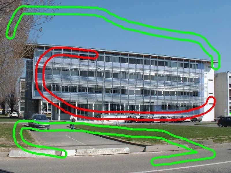
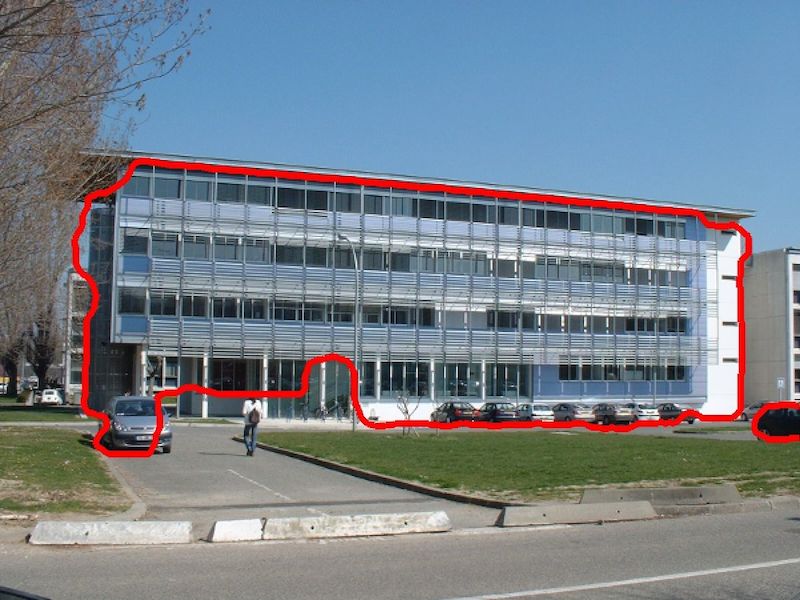
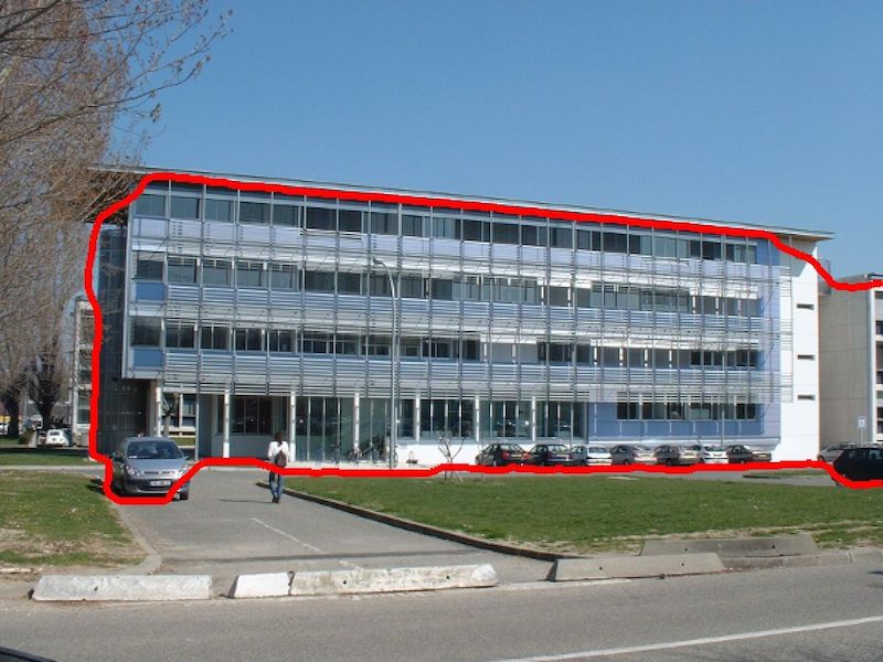
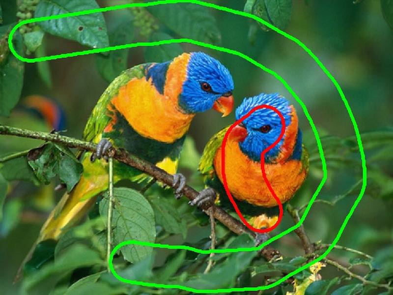
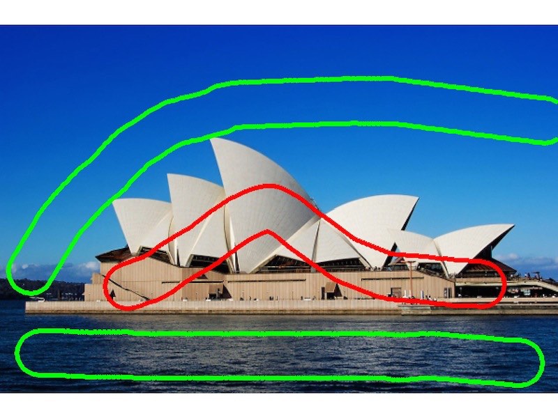
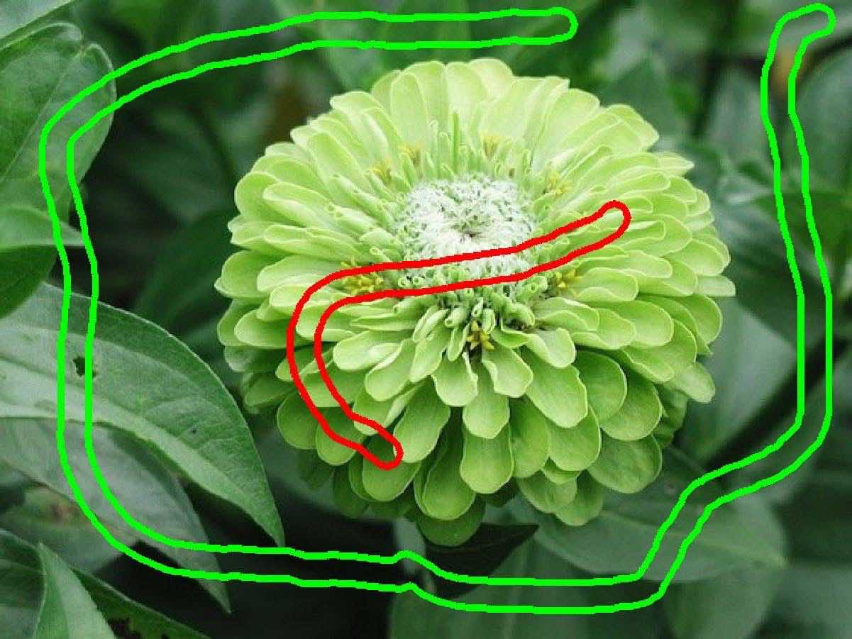
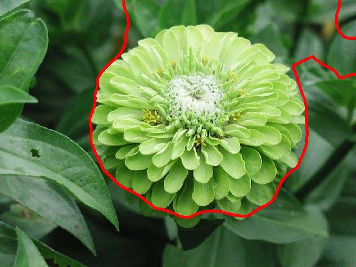
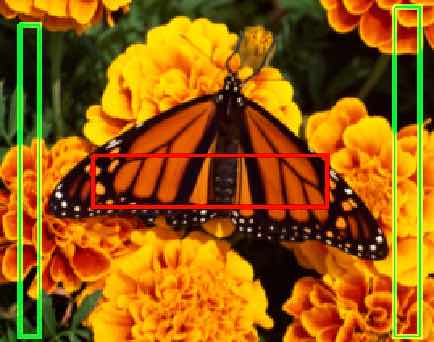
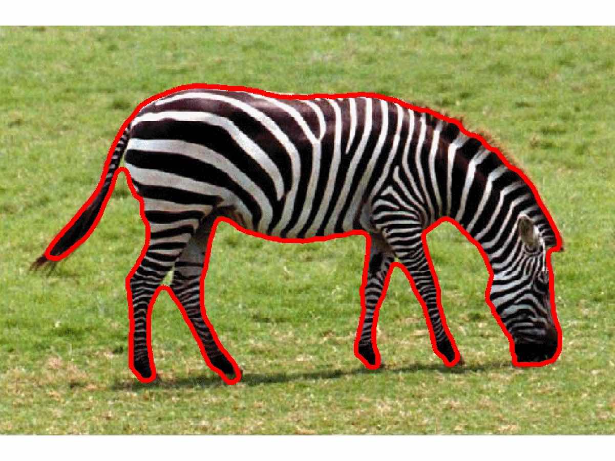
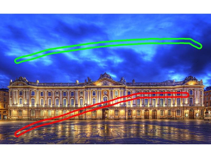
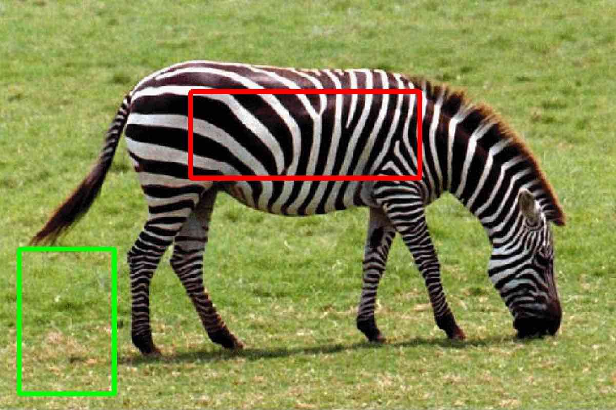
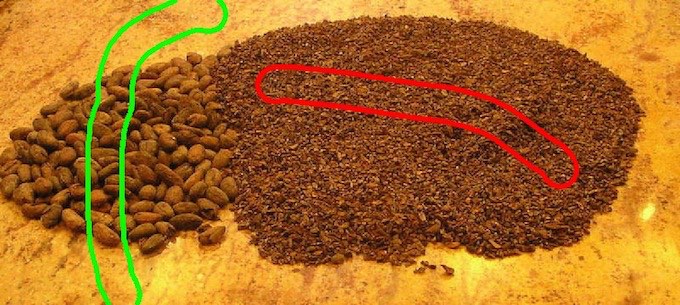
In this experimental section, exemplar regions are defined by the user with scribbles (see for instance Fig. 3) or bounding boxes (Fig. 8). These regions are only used to built prior histograms, so erroneous labelling is tolerated. The histograms $a$ and $b$ are built using hard-assignment on $M=8^{n}$ clusters, which are obtained with the K-means algorithm.

We use either RGB color features (${\cal F}=\mathrm{Id}$ and $n=d=3$) or the gradient norm of color features (${\cal F}=\lVert{D}.\rVert$ computed on each color channel, so that $n=3$). The cost matrix is defined from the Euclidean metric $\lVert\cdot\rVert$ in $\mathbb{R}^{n}$ space, combined with the concave function $1-e^{-\gamma{\lVert\cdot\rVert}{}}$, which is known to be more robust to outliers (Rubner2000, ). Approximately $1$ minute is required to run $500$ iterations and segment a 1 Megapixel color image.

To account for the case where a region boundary coincide with the image border $\partial\Omega$, we enlarge the size of the domain $\Omega$ by 1 pixel and we force variable $u$ to be null on the border. That way, the model does not favor regions that lie across the boundary.

Throughout the experiments, the diagonal preconditioning is defined using Formula (18) with $r=\delta=1$. We have observed an impressive convergence acceleration (approximately 3 orders of magnitude) due to preconditioning.

Projection onto the simplex

The projector onto the discrete probability set ${\cal S}_{1,K}$ can be computed in linear time complexity, see for instance (Condat_Simplex, ).

Thresholding

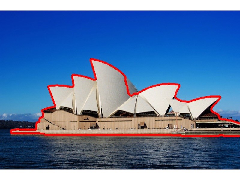
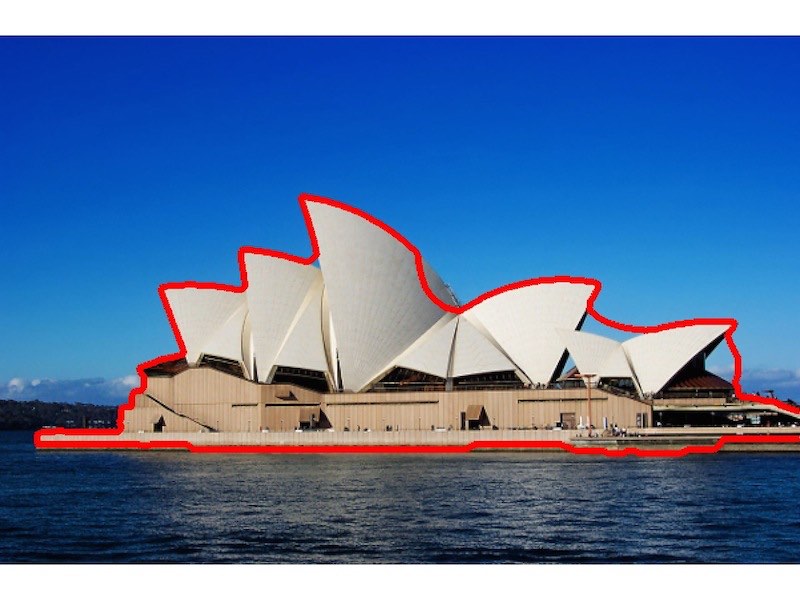
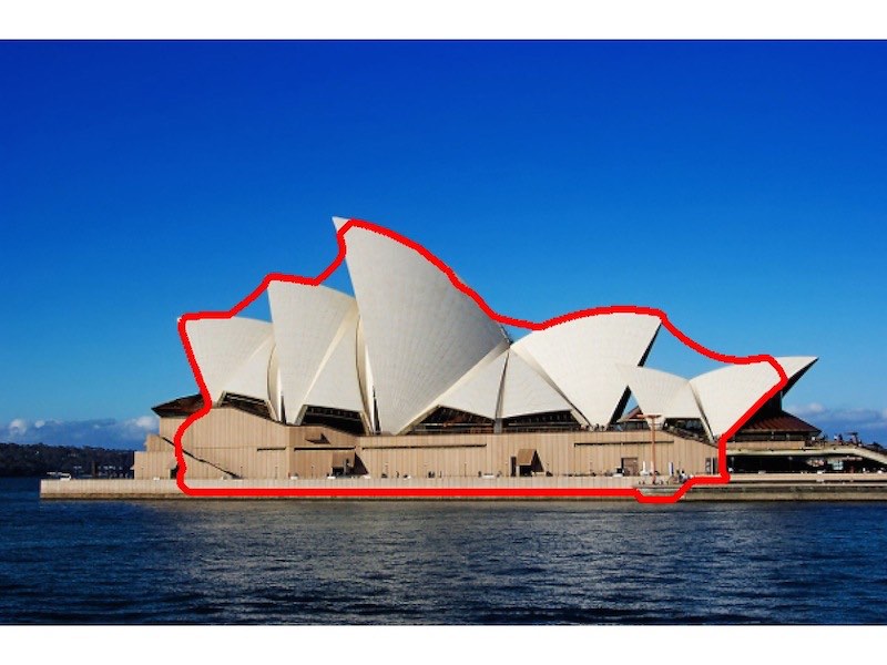
As previously stated, the segmentation map $u^{*}$ obtained by minimizing the functional (8) is not binary in general. The final segmentation is obtained by thresholding the global minima $u^{\star}$ with $t=\tfrac{1}{2}$ (see Section 2.7). This leads to the best compromise in our experiments, as illustrated in Figure 3 that shows the influence of the threshold $t$ used to get a binary segmentation.

Input	$u$	$t=0.5$
$t=0.1$	$t=0.2$	$t=0.9$

Figure 3: Illustration of the image segmentation method with MK transport cost and the influence of the final threshold parameter $t$ on the segmentation result. The user defines scribbles which indicates the object to be segmented (here in red) and the background to be discarded (in green). The output image $u$ is a regularized weight map that gives the probability of a pixel to belong to the object. This probability map $u$ is finally thresholded with a parameter $t$ to segment the input image into a region $R_{t}(u)$, which contour is displayed in red.  

5.1 Regularized vs non-regularized MK distances

As previously discussed in Section 4.7, the solutions when using the gradient of $\textbf{MK}_{\lambda,\leq N}$ or the proximity operator based on $\textbf{MK}_{\lambda,N}$ are the same when $N=|\Omega|$, even if the respective optimization schemes are different. As a consequence, we simply denote by $\textbf{MK}_{\lambda}$ when referring to these methods. We also indicates MK or $\lambda=\infty$ when not using any regularization.

We first illustrate the influence of the $\lambda$ parameter in the regularized distance $\textbf{MK}_{\lambda}$. Figure 2 gives a comparison between the non-regularized model, quite fast but using high dimensional representation (28), with the regularized model, using either a smooth low dimensional formulation (41) or a smooth high dimensional representation (46). One can see that setting a large value of $\lambda$ gives interesting results. On the other hand, using a very small value of $\lambda$ always yields poor segmentation results. In practice, if not specified otherwise, we consider $\lambda=100$ in our experiments, as higher values may lead to numerical issues (floating point precision).

5.2 Comparisons with other segmentation models including Wasserstein distance

We first exhibit the advantage of considering global data terms over histograms, such as in Eq. (2). We present a comparison with the convex model proposed in (bresson_wasserstein09, ) that includes a local data term over color distributions:

$$\begin{split}\tilde{E}(u)=\rho\mathop{{TV}}(u)+\sum_{x\in\Omega}&\;\;\textbf{MK}(a,h_{V(x)})u(x)\\ +&\;\;\textbf{MK}(b,h_{V(x)})(1-u(x))\end{split}$$

where $h_{V(x)}$ is the color distribution over the neighborhood $V(x)$ of pixel $x$. This model, that can be optimized globally (Yildi12, ), measures the local color distribution of the image with respect to the reference foreground and background distributions $a$ and $b$. As illustrated in Figure 4, such local model is not able to perform a global segmentation. Here the orange colors are more probable in the region related to the butterfly, so in small neighborhoods the flowers are classified as the butterfly, and the darker regions are segmented as being in the background. This example illustrates the importance of considering global histogram comparisons to get a global segmentation of an image. Indeed, the global distance between histograms (c) is able to recover the butterfly, whereas the local approach (b) completely fails. Local approaches are therefore only relevant when the local histograms correctly approximate the global ones.

(a) $I$, $\color[rgb]{1,0,0}\definecolor[named]{pgfstrokecolor}{rgb}{1,0,0}a$, $\color[rgb]{0,1,0}\definecolor[named]{pgfstrokecolor}{rgb}{0,1,0}b$	(b) Local (bresson_wasserstein09, )	(c) Global

Figure 4: Comparison with a local model. (a) Input image and regions where reference distributions $a$ and $b$ are estimated. The segmentation fails for the local histogram model (b) as it classifies the orange areas in the first class and the darker ones in the second class. The global histograms on the segmented zones are not close to the given ones, contrary to the global model (c).  

Inputs	$\ell_{1}$	$\lambda=\infty$	$\lambda=1000$

Figure 5: Comparison of the segmentation results obtained from the proposed segmentation models (using $\textbf{MK}_{\lambda}$ distances) together with the $\ell_{1}$ distance used in (papa_aujol, ), for different initialization. The same regularization parameter $\rho$ is used for every segmentations. Note that the optimal transport similarity measure is a more robust statistical metric between histograms than $\ell_{1}$.  

(a) Initialization	(b) Result

Figure 6: Comparison with a non convex model. The Wasserstein active contours method (PeyreWassersteinSeg12, ), initialized in two different ways in (a), provides the corresponding segmentations presented in (b), illustrating the non-convexity of the model. When carefully parameterized, it leads to a segmentation close to the one obtained with our global approach (see Figure 4(c)).  

Next, we illustrate the advantage of having a convex model that does not depend on the initialization. We compare our results with the ones obtained with the Wasserstein Active Contour method proposed in (PeyreWassersteinSeg12, ). Such approach consists in deforming a level set function in order to minimize globally the Wasserstein distance between the reference histograms and the one induced by the segmentation. To make the level set evolve, this formulation requires complex shape gradients computations. As illustrated in Figure 6, even if this model can give good segmentations that are close to the ones we obtained in Figure 4 (c), its initialization may be a critical step as really different segmentations are obtained with very similar initializations.

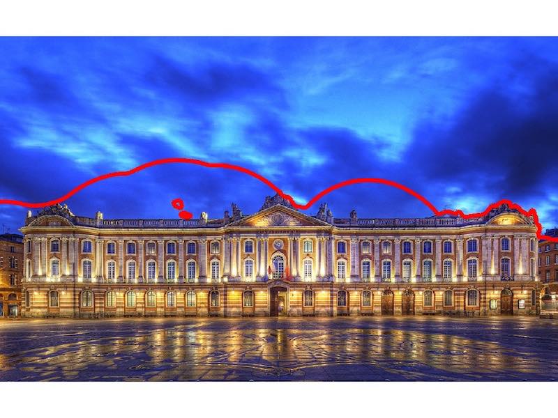
We finally show comparisons with the global model of (papa_aujol, ) that includes $\ell_{1}$ distances between histograms. Figure 5 first illustrates the robustness of optimal transport distance with respect to bin-to-bin $\ell_{1}$ distance. A small variation of the reference histograms may involve a large change in the final segmentation wit $\ell_{1}$ distance, whereas segmentations obtained with MK or regularized $\textbf{MK}_{\lambda}$ are stable.

Input
$\ell_{1}$	MK

Figure 7: Robustness of MK with respect to $\ell_{1}$. The blue colors that are not in the reference histograms are considered correctly as background with MK distance, but as foreground with the $\ell_{1}$ model where no color comparison is performed.  

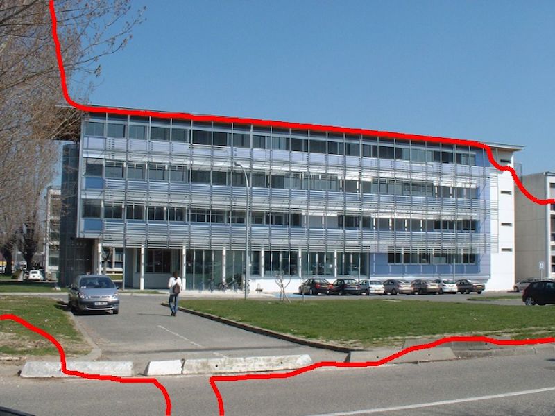
Contrary to optimal transport, when a color is not present in the reference histograms, the $\ell_{1}$ distance does not take into account the color similarity between different bins, which can lead to incorrect segmentation. This is illustrated with the blue colors in Figure 7 where the $\ell_{1}$ distance leads to an incorrect segmentation by associating some blue tones to the building area.

5.3 General results

The robustness of optimal transport distances is further illustrated in Figure 8. It is indeed possible to use a prior histogram from a different image, even with a different clustering of the feature space. This is not possible with a bin-to-bin metric, such as $\ell_{1}$, which requires the same clustering.

Input histograms	Segmentation $1$
Segmentation $2$	Segmentation $3$

Figure 8: Illustration of the interest of optimal transport cost for the comparison of histograms. Its robustness makes it possible to use prior histograms from different images (in this exemple, histograms are estimated from image $1$ and used to segment all images).  

Other examples on texture segmentation are presented in Figure 9 where the proposed method is perfectly able to recover the textured areas. We considered here the joint histogram of gradient norms on the $3$ color channels. The complexity of the algorithm is the same as for color features, as long as we use the same number of clusters to quantize the feature space.

Input	MK

Figure 9: Texture segmentation using joint histograms of color gradient norms. In this exemple, only gradient information is taken into account, illustrating the versatility of the optimal transport framework.  

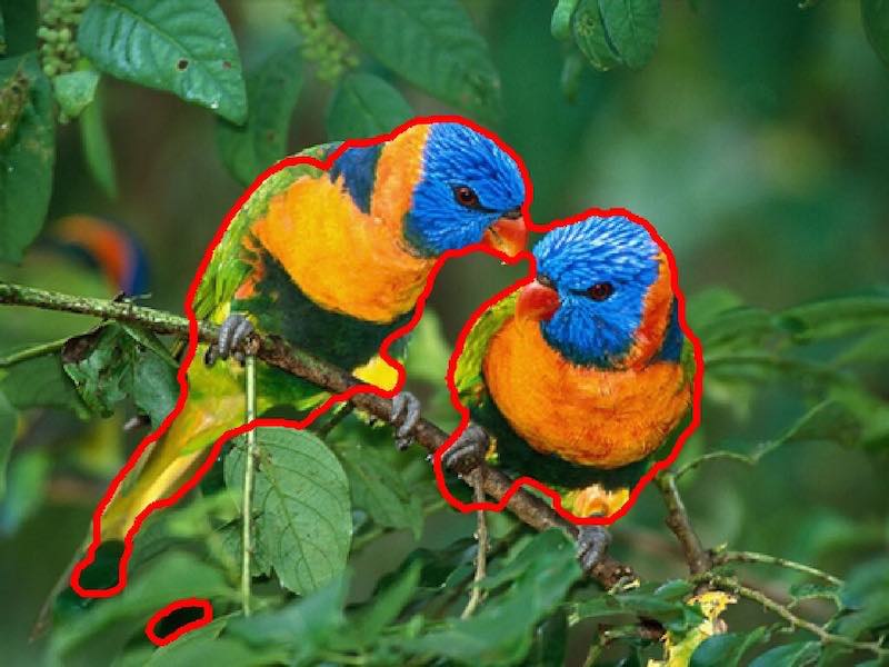
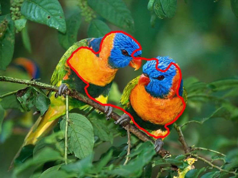
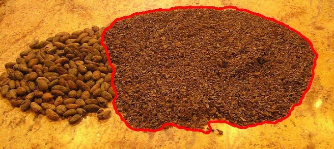
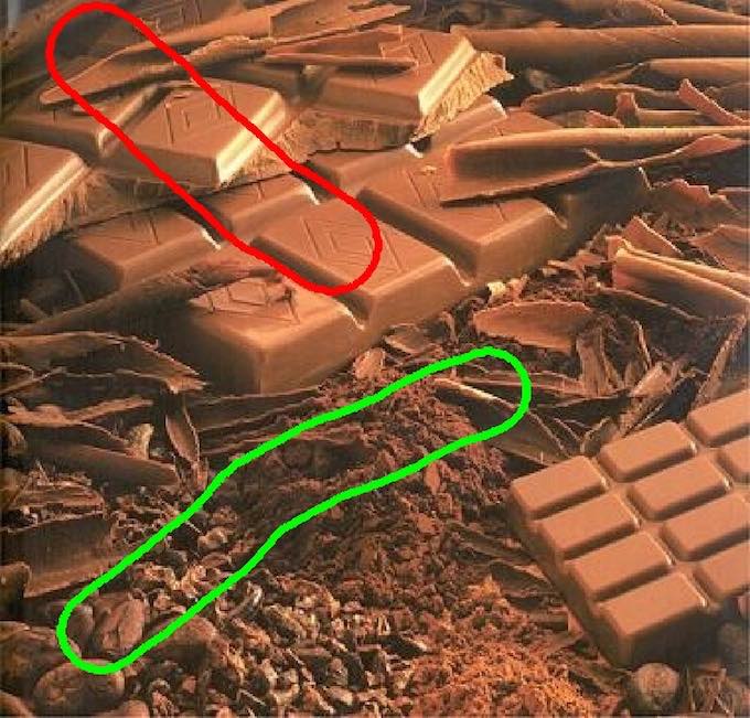
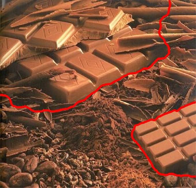
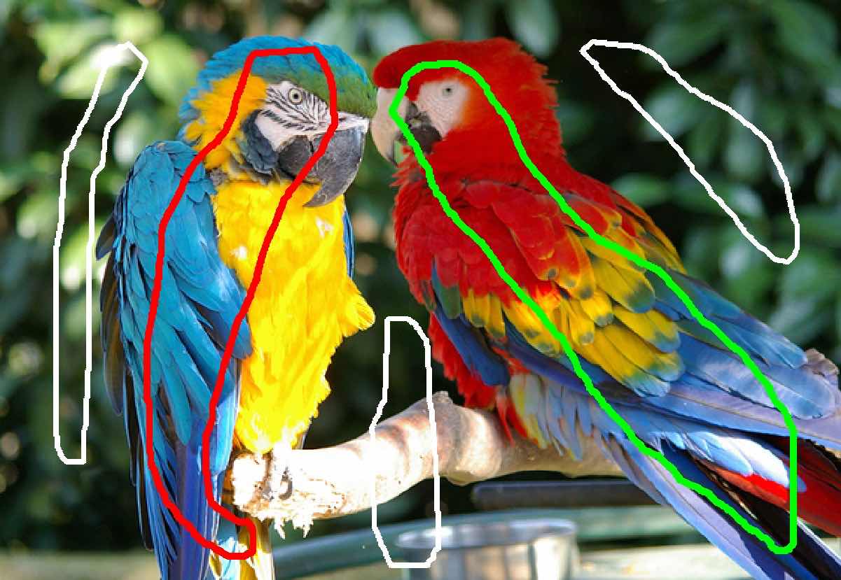
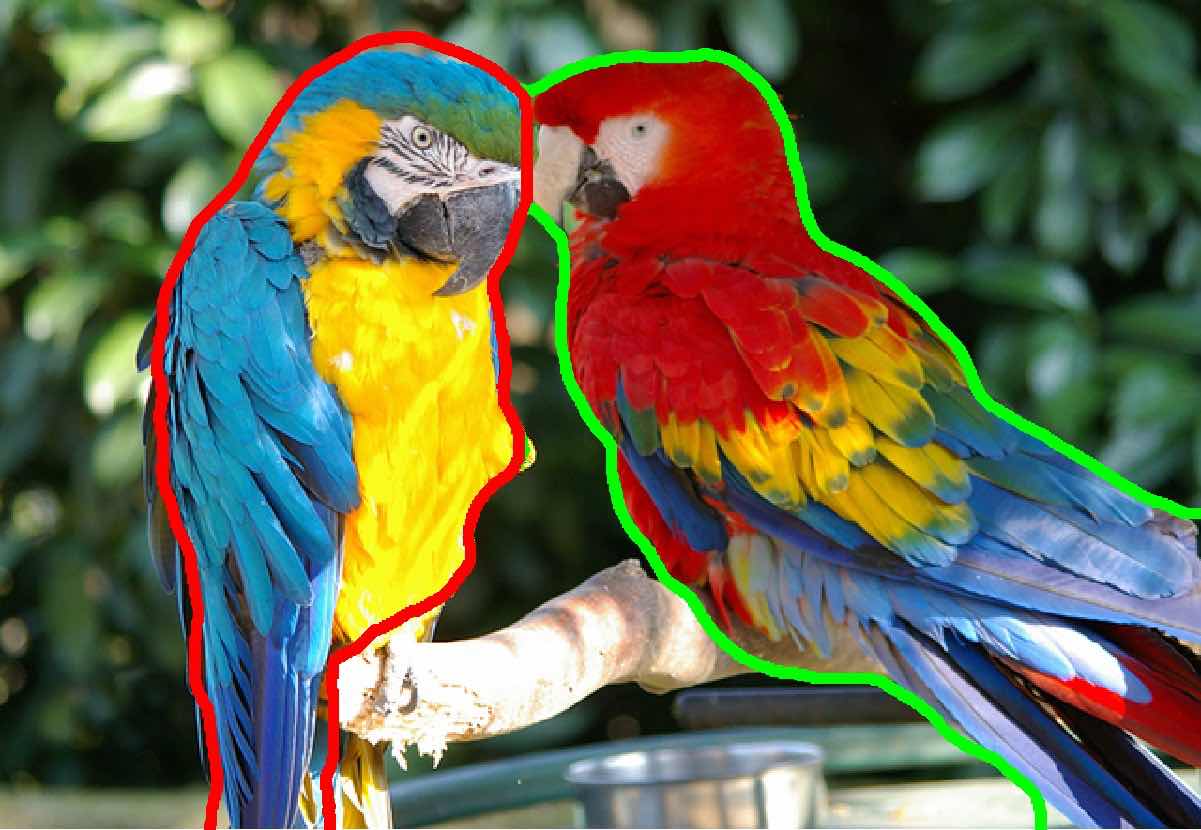
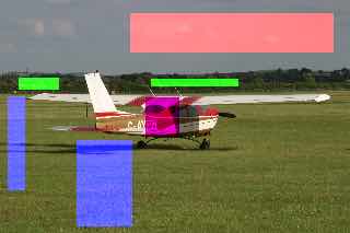
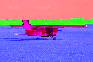
We finally present experiments involving more than two partitions in Figure 10. In the first line, three regions are considered for the background and the two parrots. Even if the two parrots share similar colors, the model is able to find a global segmentation of the image in three regions. In the second line of Figure 10, we considered $4$ regions for the sky, the grass, the forest and the plane. The approach is able to deal with the color variations inside each class in order to perform a correct segmentation.

Input	Segmentation

Figure 10: Multi-phase segmentation with $3$ regions (first line) and $4$ regions (second line).  

6 Unsupervised Co-segmentation

In this section, we extend our framework to the unsupervised co-segmentation of multiple images. We invite the reader to see the following reference (Vicente_co-seg_eccv10, ) for a complete review.

6.1 Co-segmentation of $2$ images

We first consider two images $I^{1}$ and $I^{2}$ the domain of which is respectively $\Omega_{1}$ and $\Omega_{2}$ composed of $N_{1}$ and $N_{2}$ pixels. Assuming that the images contain a common object, the goal is now to jointly segment them without any additional prior.

Model for two images

To that end, following the model used in (Vicente_co-seg_eccv10, ; Swoboda13, ), we aim at finding the largest regions that have similar feature distributions. To define the segmentation maps $u^{1}$ and $u^{2}$ related to each image, we consider the following model first investigated in (coseg_hist_matching, ; coseg_hist_matching_L2, ), denoting $u=(u^{1};u^{2})$:

$$J^{\prime}(u):={S}\left(H_{1}u^{1},H_{2}u^{2}\right)+\sum_{k=1}^{2}\rho\mathop{{TV}}(u^{k})-\delta{|\!|u^{k}|\!|}_{1}$$ (47)

where, for a non-negative variable $u^{k}$ we have a total mass ${|\!|u^{k}|\!|}_{1}=\langle u^{k},\,\mathbf{1}_{N_{k}}\rangle$. When $u^{k}\in\{0,1\}^{N_{k}}$, this term corresponds to the area of the region segmented in image $I^{k}$. Such a ballooning term encourages the segmentation of large regions. Without this term, a global optimum would be given by $u^{k}=\mathbf{0}$.

Following definition (5), the operator $H_{k}(i,x)$ is $1$ if pixel $I^{k}(x)$ belongs to the cluster ${\cal C}_{{\cal X}_{k}}(i)$ and $0$ otherwise. As before, the value of the segmentation variables $u^{k}$ are relaxed into the convex intervals $[0,1]^{N_{k}}$.

In (Vicente_co-seg_eccv10, ), several cost functions ${S}$ are benchmarked for the model defined in Eq. (47), such as $\ell_{1}$ and $\ell_{2}$. It is demonstrated that $\ell_{1}$ performs the best. In (Swoboda13, ), Wasserstein distance is used again to measure the similarity of the two histograms. In the following, we investigate the use of these two metrics in our setting.

Property of the segmented regions

To begin with, note that when considering optimal transport cost to define ${S}$, one has to constraint the histograms to have the same mass, i.e. $(H_{1}u^{1},H_{2}u^{2})\in{\Delta}$. When using assignment operators such as in (5), this boils down to constraint the segmentation variables to have the same mass, i.e. $\langle u^{1},\,\mathbf{1}_{N_{1}}\rangle=\langle u^{2},\,\mathbf{1}_{N_{2}}\rangle$.

When looking for a binary solution, this condition implies that the two regions corresponding to the segmentation of each image have the exact same number of pixels. This means that the model is not robust to small scale change in appearance with optimal cost transport, while is it the case when using the $\ell_{1}$ metric, as demonstrated in (Vicente_co-seg_eccv10, ). In practice, while this property does not necessarily hold for solutions of the relaxed problem that are binarized by thresholding (see Eq. (4)), this limitation has been also observed.

One simple way to remove such restriction from the model is to use the same formulation introduced in Section 2.3.3 for segmentation. Unfortunately this boils down to define the similarity measure with

$$S(H_{1}u_{1}\langle u_{2},\,\mathbf{1}\rangle,H_{2}u_{2}\langle u_{1},\,\mathbf{1}\rangle)$$

which is obviously non-convex and does not fit the optimization framework used in this paper.

It is not the first time that the conservation of mass in the optimal transport framework is reported to limit its practical interest in imaging problem, and several variations have been proposed to circumvent it. Without entering into details, a common idea is to discard the conservation of mass when the two histograms are unbalanced and to define alternative transport maps that may create or annihilate mass. As an exemple, a solution might be to transport the minimum amount of mass between the unnormalized histograms and penalize the remaining, as done by the distance introduced in (Pele-ICCV, ) and similarly in (gramfort_2015, ). Other models has been recently investigated, such as in (lombardi_maitre_2013, ), and (Vialard15b, ; Frogner, ). However, the application of such metric for our setting is far from being straightforward and need careful analysis that is left for future work.

Optimization

To solve the relaxed problem

$$\min_{u\in[0,1]^{N_{1}+N_{2}}}J^{\prime}(u)$$

using either $\ell_{1}$, MK or $\textbf{MK}_{\lambda}$ as a cost function ${S}$, we rely again on the primal-dual formulation (14) of the problem and the algorithm (15). Notice that the minor difference with previous segmentation problems is the presence of the linear ballooning term and that there is only one dissimilarity term.

Experiments

We now illustrate the behavior of this model. Again, we underline that the convex cosegmentation model (47) is not new, as our approach only differ algorithmically from (Vicente_co-seg_eccv10, ; Swoboda13, ) when using $\ell_{1}$ or MK as a cost function. Therefore, we only focus on results obtained using optimal transport with entropic regularization (setting $\lambda=100$).

In the synthetic experiment of Figure 11 containing exactly the same object with different backgrounds, we compare our approach with the one of (Swoboda13, ), that does not include entropic regularization. Both methods gives similar co-segmentations.

Figure 11: Co-segmentation and optimal transport with or without entropic regularization. The results obtained with the model (47) with the entropic regularization (in red), that approximate the method of (Swoboda13, ) (in yellow, image courtesy of (Swoboda13, )). The estimated segmentation maps ${u^{k}}$ are binary almost everywhere. The threshold $t=\frac{1}{2}$ is used to obtain the final co-segmentation regions.  

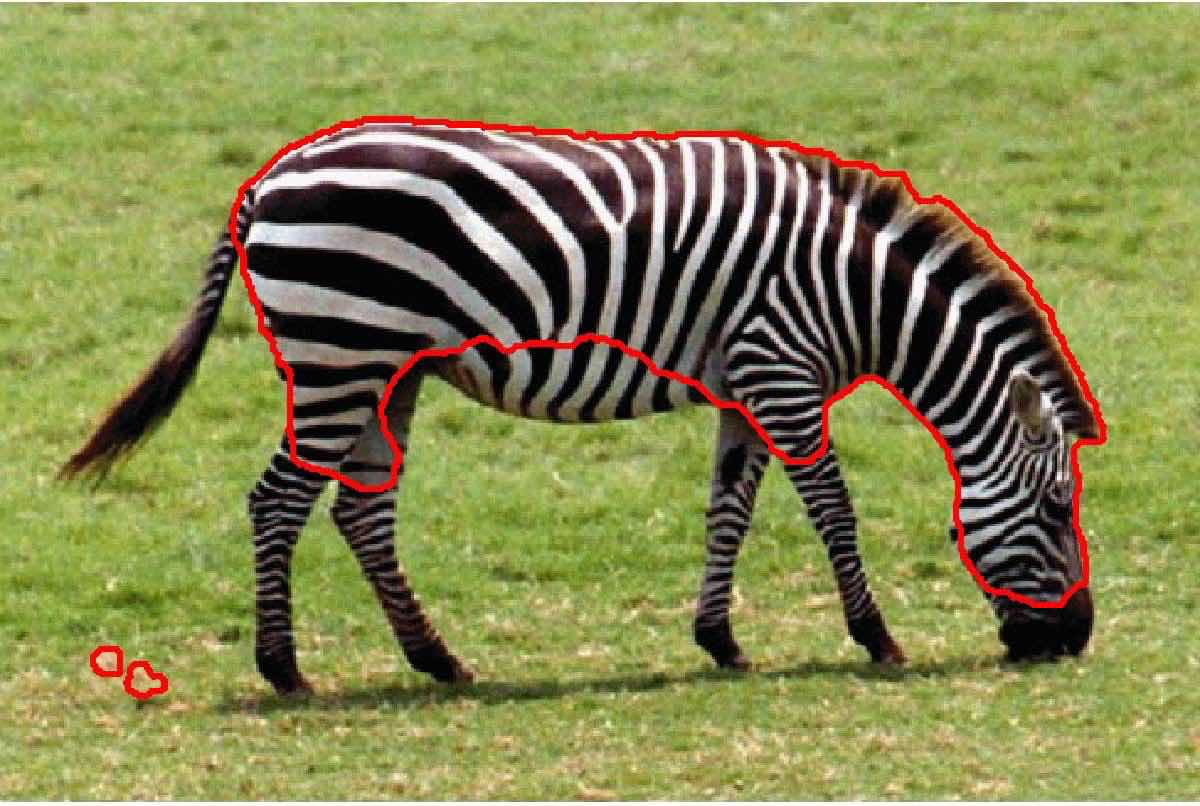
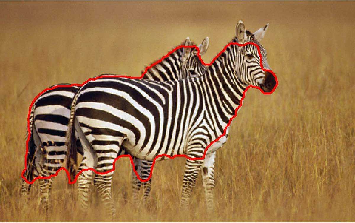
When considering images where the common object has a similar scale in both images, Figure 12 shows that the condition $|\!|u^{1}|\!|_{1}=|\!|u^{2}|\!|_{1}$ is not restrictive and our method still gives acceptable co-segmentations.

$u^{1}$	$u^{2}$

Figure 12: Co-segmentation of two zebras with the model (47). The convex constraint $|\!|u^{1}|\!|_{1}=|\!|u^{2}|\!|_{1}$ enforces the segmented regions to have the same area. As the obtained result is not binary, the areas may be different after the thresholding.  

Nevertheless, in a more general setting, we cannot expect the common objects to have the same scale in all images. We leave the study of alternative optimal transport based distance such as (Vialard15b, ; Frogner, ) for future work.

6.2 Co-segmentation of $P$ images

We consider now the generalization of the previous co-segmentation model to an arbitrary number of $P\geq 2$ images.

Complexity

A natural extension of (47) for more than two images would be to penalize the average dissimilarity between all image pairs, writing for instance

$$\begin{split}J^{\prime\prime}(u)&=\sum_{k=1}^{P-1}\left(\sum_{l=k+1}^{P}S(H_{k}u^{k},H_{l}u^{l})\right)+\rho\mathop{{TV}}(u^{k})\\ &\quad-\delta{|\!|u^{k}|\!|}_{1}+\chi_{[0,1]^{N_{k}}}(u^{k})\end{split}$$ (48)

which would require to compute $\tiny\begin{pmatrix}P\\ 2\end{pmatrix}$ similarity terms $S(H_{k}u^{k},H_{l}u^{l})$. However, the complexity of such a model scales quadratically with the number of images $P$ which is not desirable.

To that end, we consider instead the following barycentric formulation which scales linearly with $P$

$$\begin{split}J^{\prime\prime\prime}(u,b)&=\sum_{k=1}^{P}S(H_{k}u^{k},b)+\rho\mathop{{TV}}(u^{k})\\ &\quad-\delta{|\!|u^{k}|\!|}_{1}+\chi_{[0,1]^{N_{k}}}(u^{k})+\chi_{\geq\mathbf{0}}(b)\end{split}$$ (49)

where $b$ is the estimated barycentric distribution between the histograms of the segmented regions in all images. Note that in the unsupervised case studied in this section, the barycenter $b$ has to be estimated jointly with segmentation variables.

Model properties with optimal transport costs

Combining the $O(P^{2})$ model (48) or the linear barycentric formulation (49) with optimal transport based cost functions MK and $\textbf{MK}_{\lambda}$ results in the scaling problem previously reported with model (47), as definitions of MK (24) and $\textbf{MK}_{\lambda}$ (31) constraint each pair of histograms to have the same mass. Non-convex formulation or unbalanced transport costs (Frogner, ; Vialard15b, ) should again be considered as a solution, but do not fit in the proposed optimization framework.

Model properties with $\ell_{1}$

In order to circumvent this issue, we consider the $\ell_{1}$ case instead, i.e. using

$$S(H_{k}u^{k},b)={|\!|H_{k}u^{k}-b|\!|}_{1}.$$

As stated before in paragraph 3.1, the $\ell_{1}$ distance between normalized histograms can be seen as the total variation distance, a specific instance of the MK distance that naturally extend to unnormalized histograms. In this setting, recall that histograms must have the same number of bins $M$ and the exact same feature clusters ${\cal C}_{\cal X}$ (see Section 2.3.2).

Optimization

The minimization of the functional (49) for fixed histograms $H_{k}u^{k}$ boils down to the smooth Wasserstein barycenter problem studied in (CuturiPeyre_smoothdualwasserstein, ). The authors investigate the dual formulation this primal problem and show that it can be solved by a projected gradient descent on the dual problem. They resort to a splitting strategy, defining $P$ primal histogram variables $(b_{k}\in\mathbb{R}^{M})_{k=1..P}$ with the linear constraint $b_{1}=\ldots=b_{P}.$ Using a similar approach, one obtain the following primal-dual formulation

$$\begin{split}\min_{\begin{subarray}{c}u\\[2.84526pt] b\end{subarray}}\;\max_{\begin{subarray}{c}h\\[1.42262pt] v\end{subarray}}\;&\sum_{k=1}^{P}\langle H_{k}u^{k}-b,\,h_{k}\rangle-\delta\langle u^{k},\,\mathbf{1}_{N_{k}}\rangle+\langle D_{k}u^{k},\,v_{k}\rangle\\ &\qquad-\chi_{|\!|h_{k}|\!|_{\infty}\leq 1}-\chi_{|\!|v_{k}|\!|_{\infty,2}\leq\rho}\\ &\qquad+\chi_{u^{k}\in[0;1]^{N_{k}}}+\chi_{b\geq\mathbf{0}}\end{split}$$

which fits the canonic form of Problem (14). In the above equation, $D_{k}$ refers to the finite difference operator in the grid $\Omega_{k}$ of image $I^{k}$.

The algorithm (15) requires to compute the Euclidean projector onto the nonnegative orthant (30) and on the $\ell_{\infty}$ unit ball (similarly to Eq. (16))

$${\text{Proj}}_{|\!|.|\!|_{\infty}\leq 1}(h)(i)=\frac{h(i)}{\max\{|h(i)|,1\}}.$$

Experiments

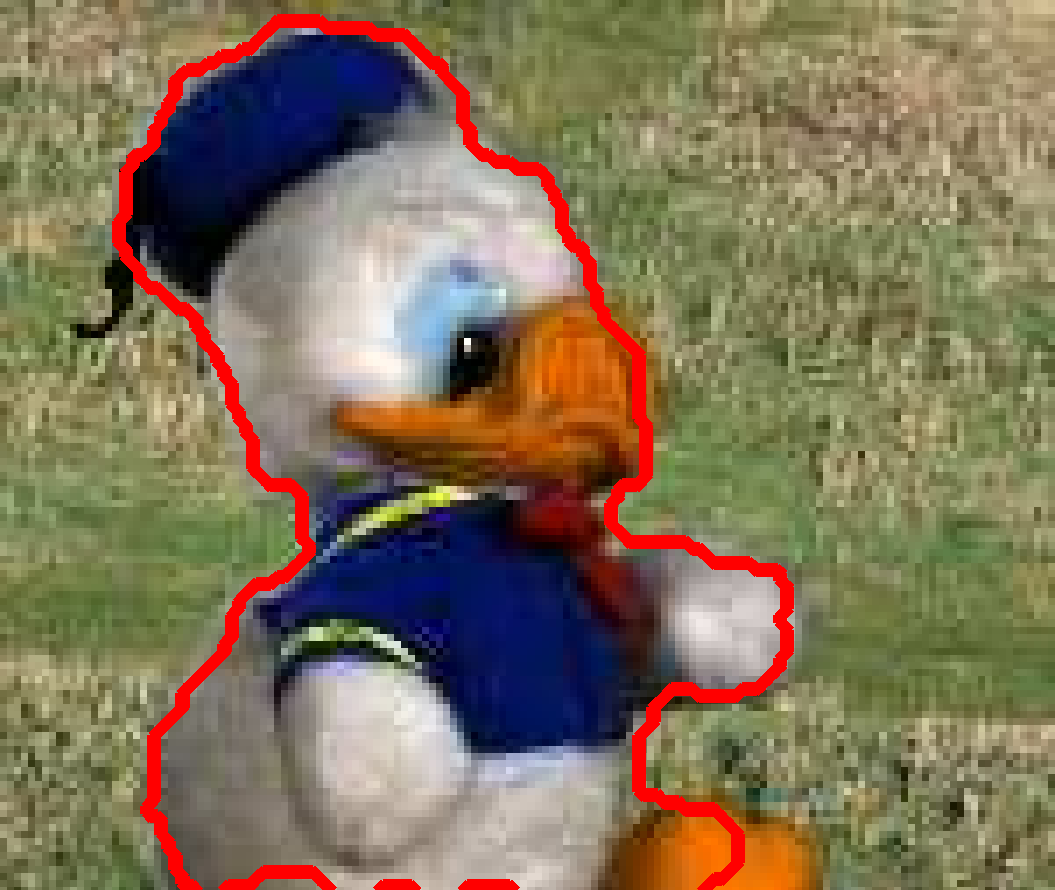
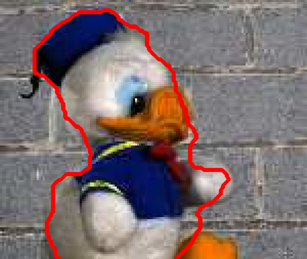
To illustrate the validity of the proposed model, we repeat the toy experiment of Figure 11 in Figure 13, where the same object is shown in two images with different backgrounds. While there is no more constraint on the size of the objects to segment as in Eq. (47), the model (49) is still able to get a good co-segmentation of the data.

Figure 13: Examples of co-segmentation of $P=2$ images with model (49). The objects to segment have the same scale. Comparing with the first line with Figure 11, results similar to the model (47) and the method (Swoboda13, ) (in yellow), whereas no constraint is considered here on the size of the regions. 

Figure 14: Co-segmentation of $P=5$ images with model (49).  

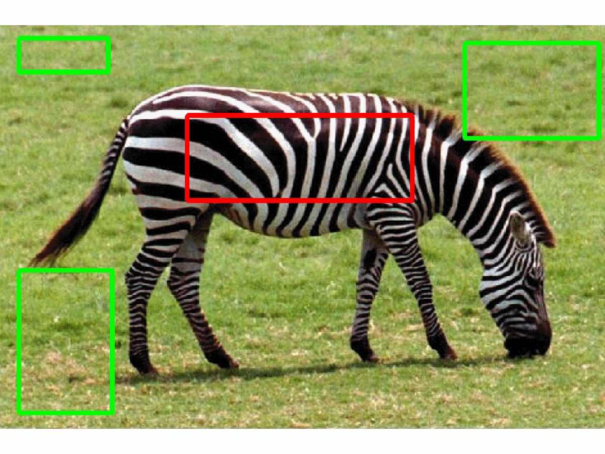
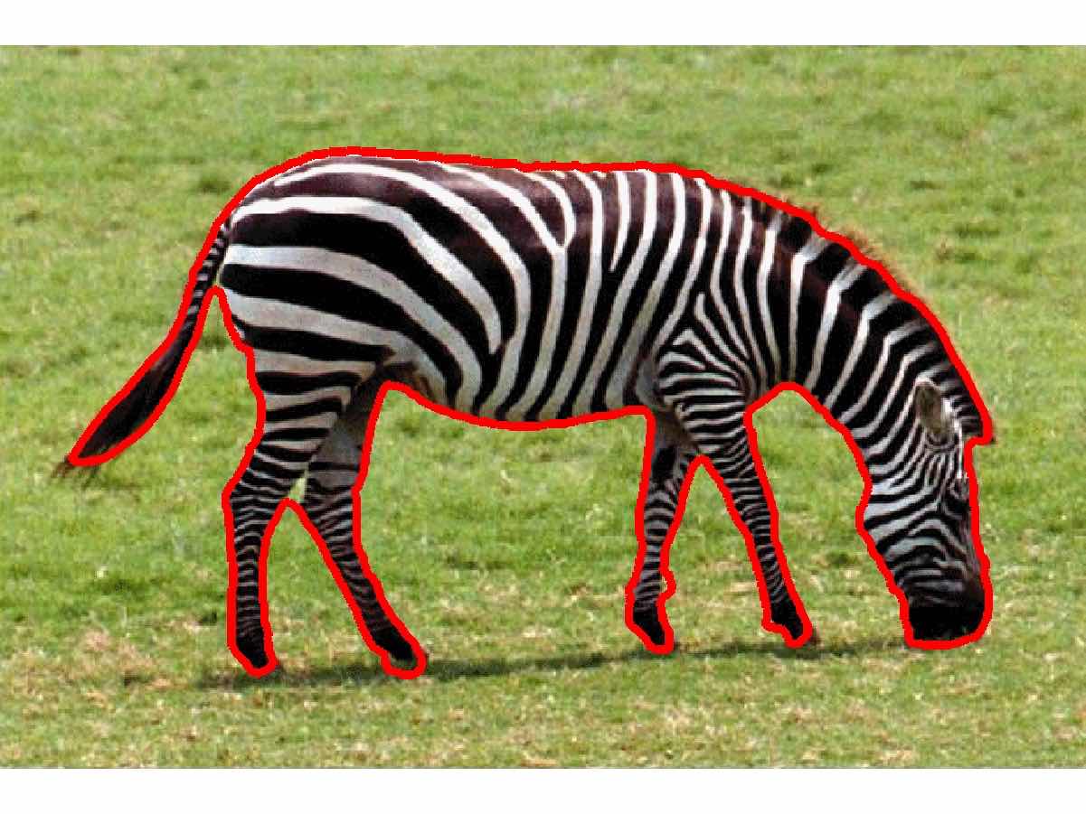
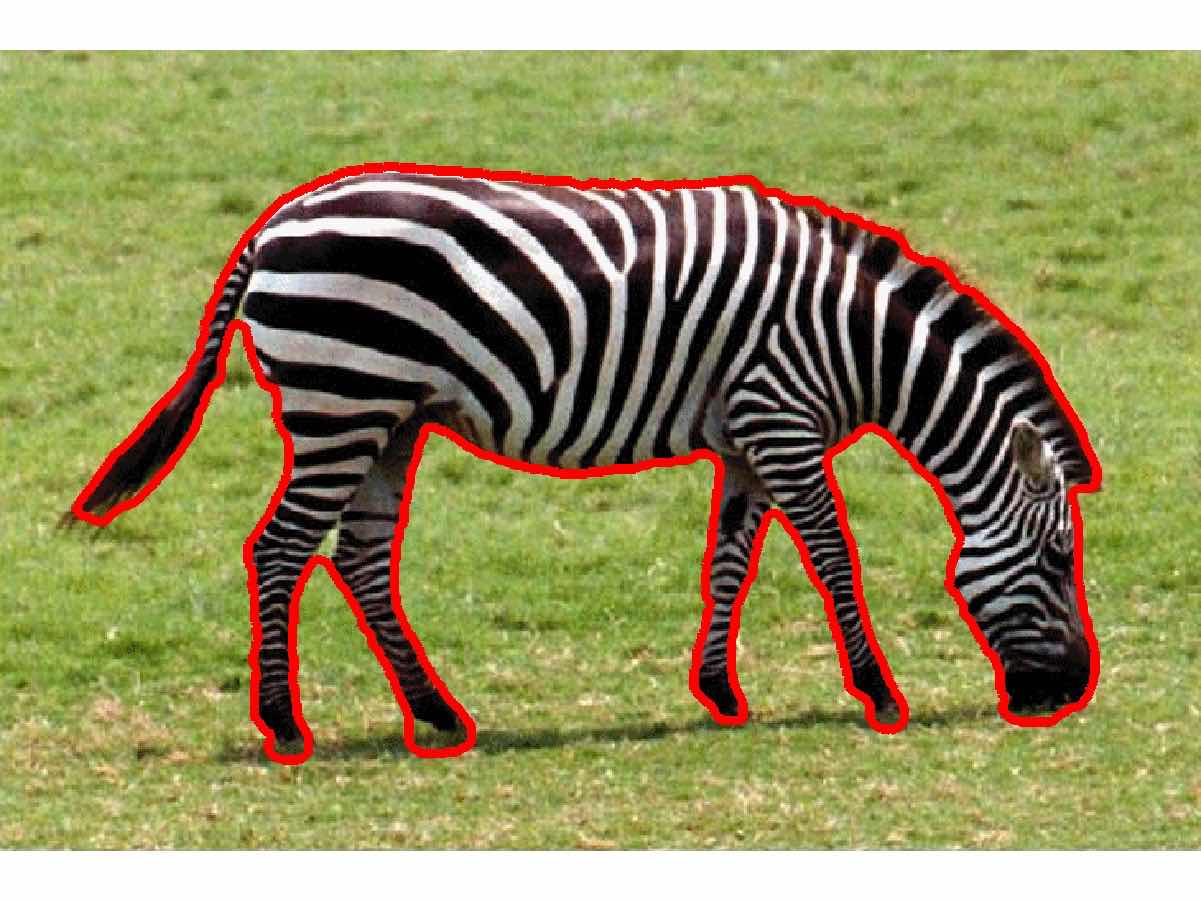
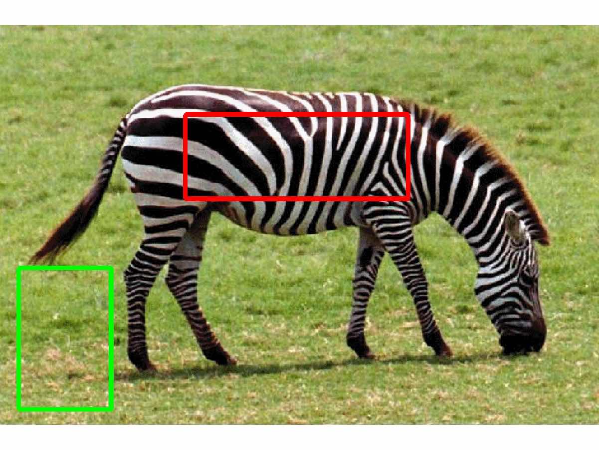
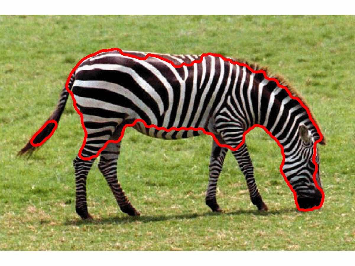
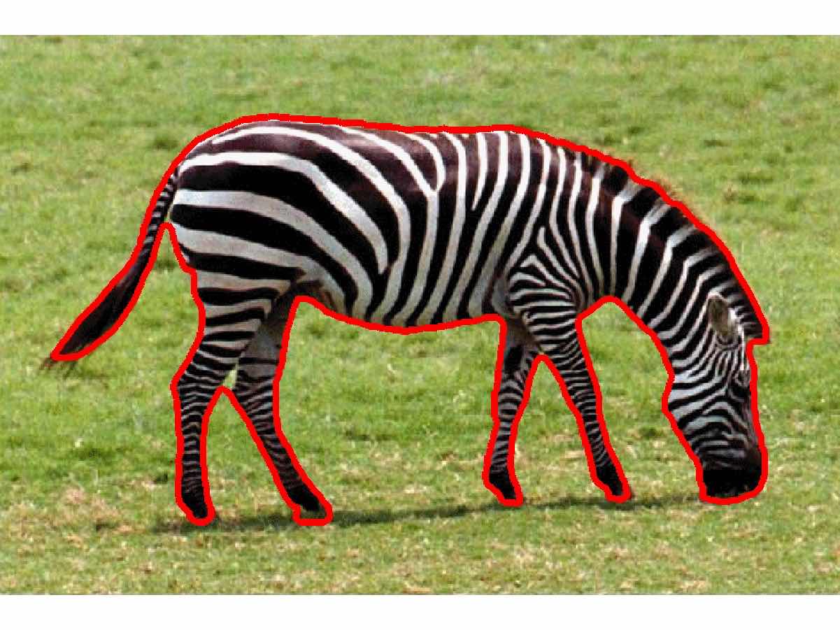
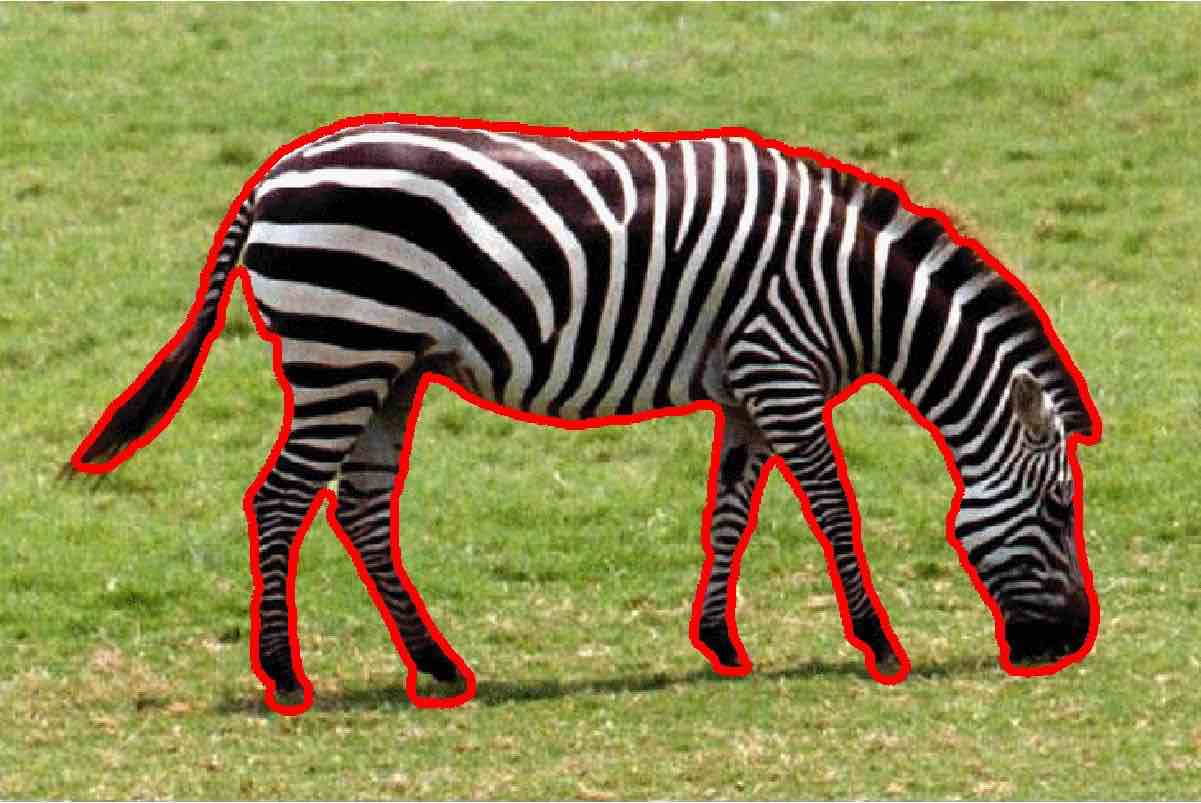
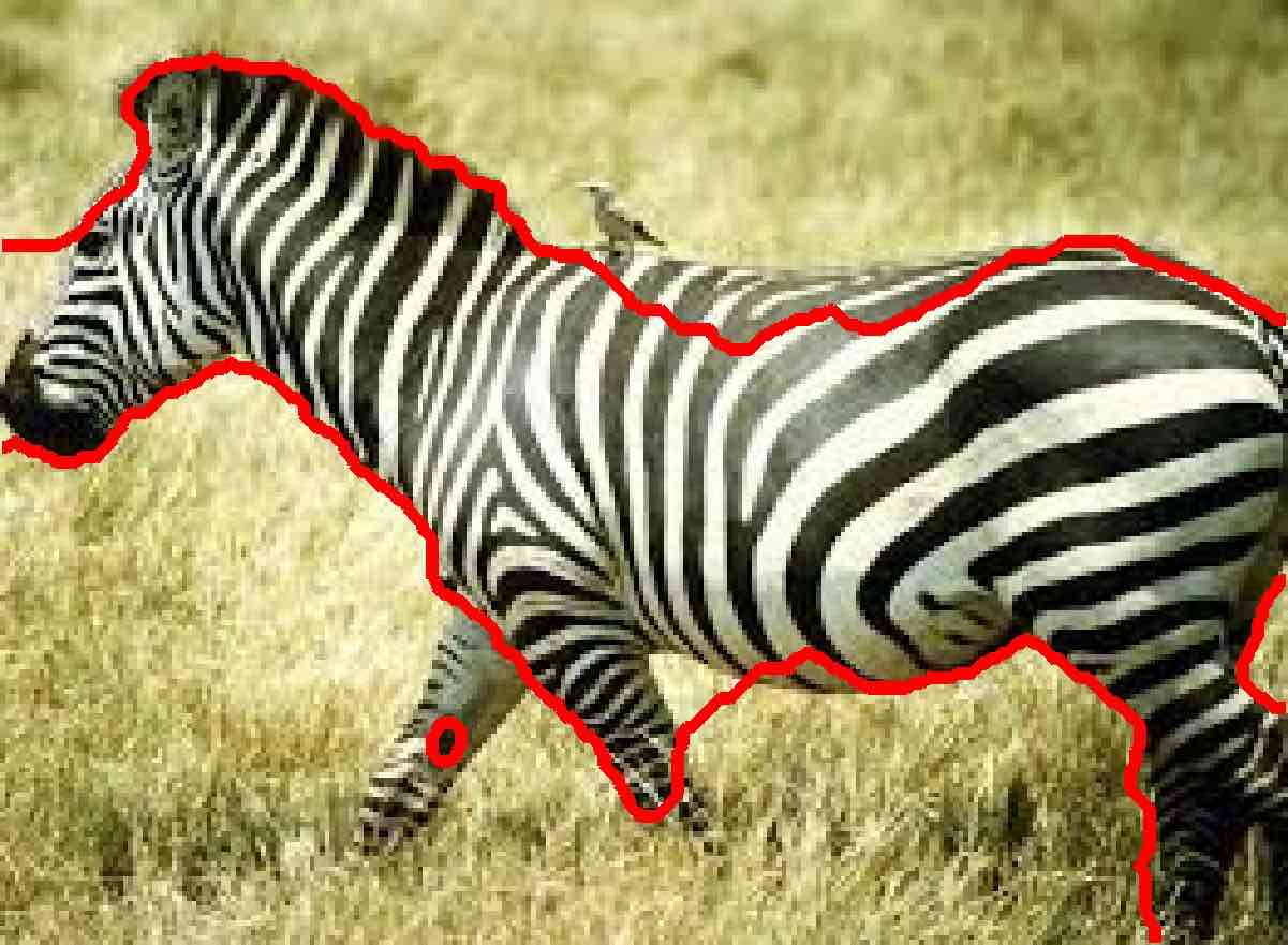
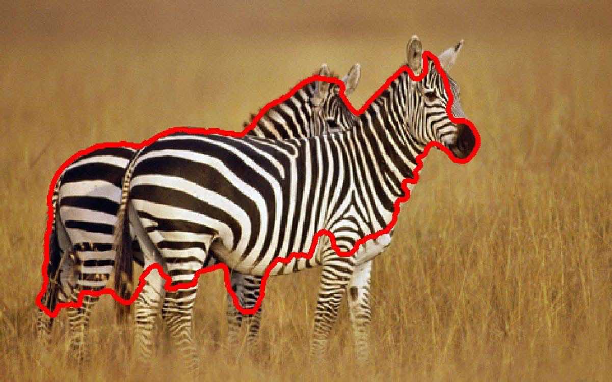
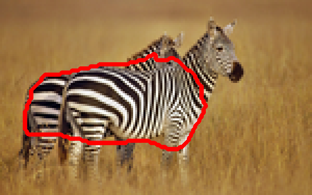
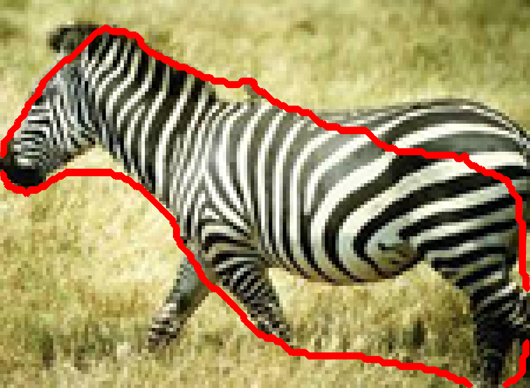
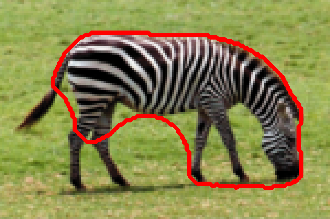
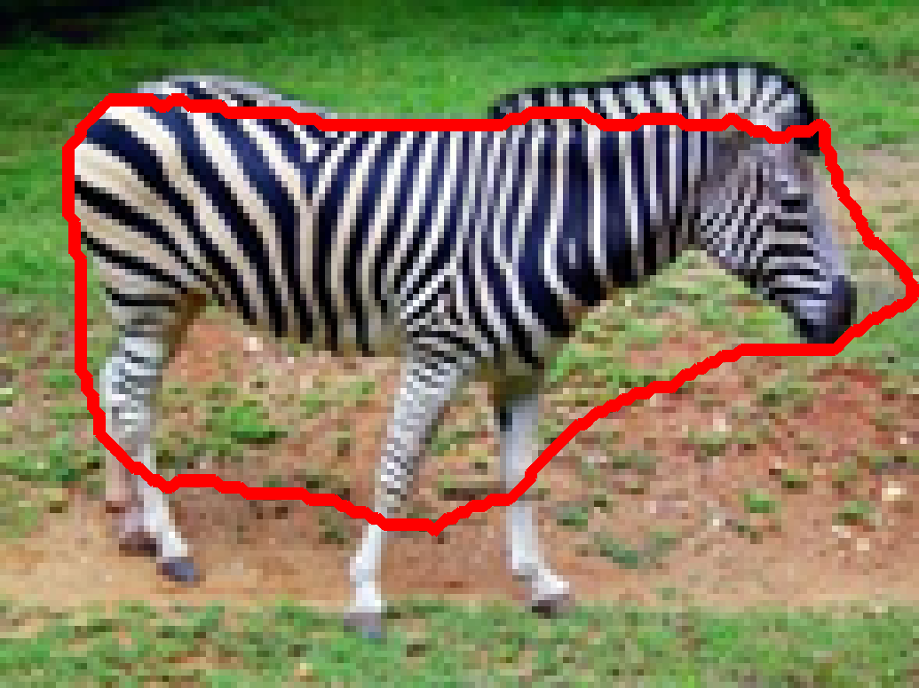
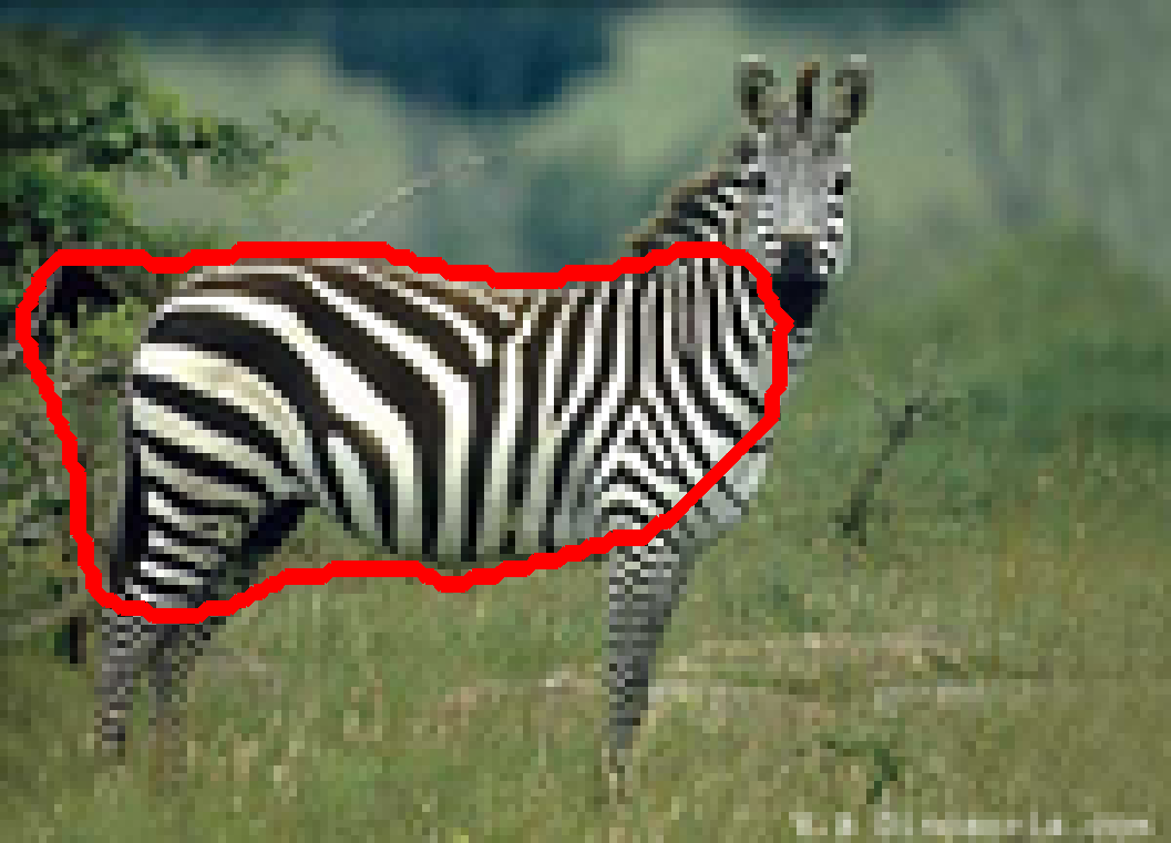
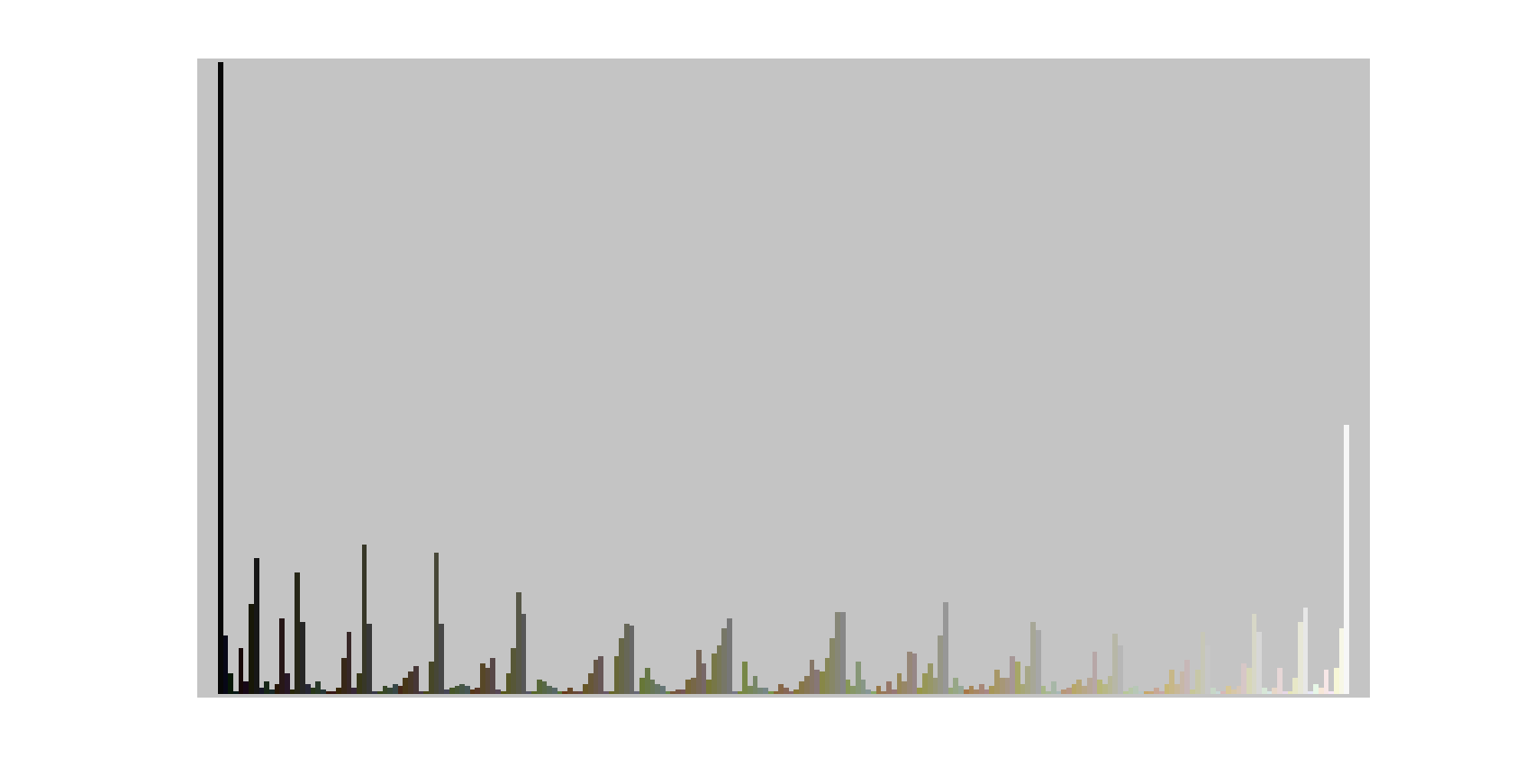
In Figure 14, we illustrate how this new model is able to segment objects of different scales in $P=5$ images. The area of the zebra can be very different in each image. Note that for simplicity the same regularization parameter $\rho$ and ballooning parameter $\delta$ are used for all images in the model (49), whereas one should tune separately these parameters according to each image in order to obtain more accurate co-segmentations. The histogram $b$ recovered from the model is shown in Figure 15.

Figure 15: Learnt barycenter histogram for Figure 14. It mainly contains black and white colors corresponding to the zebras.  

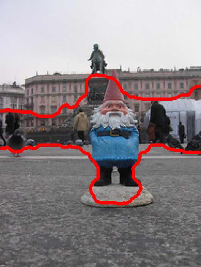
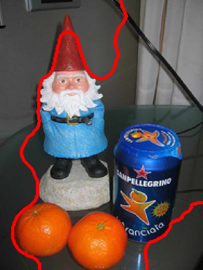
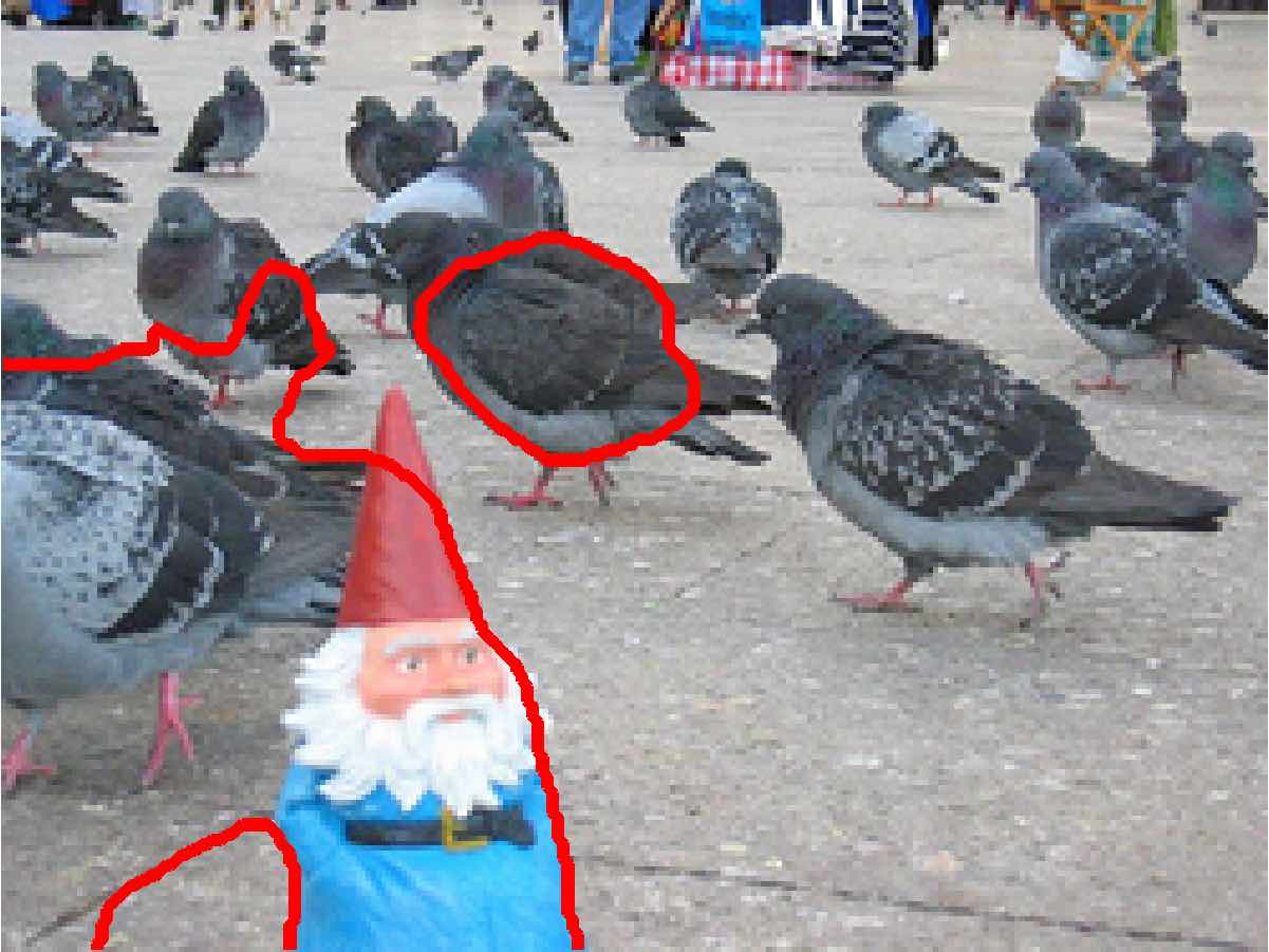
Moreover, it seems necessary to add information on the background for improving these results. In the previous examples of Figures 13 and 14, the backgrounds were enough different in the different images to be discarded by the model. As soon as the backgrounds of the co-segmented images contain very similar informations (for instance grey regions outside the gnome in images of Figure 16), the ballooning term in Eq. (49) forces the model to include these areas in the co-segmentations.

Figure 16: Incorrect co-segmentation result in case of similar backgrounds in the two images.  

7 Conclusion and future work

In this work, several formulations have been proposed to incorporate transport-based cost functions in convex variational models for supervised segmentation and unsupervised co-segmentation. The proposed framework includes entropic regularization of the optimal-transport distance, and deals with multiple objets as well as collection of images.

As already demonstrated for the image segmentation problem, optimal transport yields significative advantages when comparing feature distribution from segmented regions (robustness with respect to histogram quantization, the possibility to incorporate prior information about feature into the transport cost, definition of a metric between different types of feature, etc). When considering entropic regularization, the algorithmic scheme is yet very similar to the one obtained for the $\ell_{1}$ norm, at the only expense of requiring more memory. We observed, as acknowledged in (CuturiPeyre_smoothdualwasserstein, ), that such regularization offers practical acceleration for small histograms but also improves robustness to outliers (such as noise or rare features). However, we also emphasized that large regularization degrade significatively the performance.

The main limitation highlighted and discussed in this work is the lack of scale invariance property for the unsupervised co-segmentation problem due to the convex formulation. In comparison, non-convex formulations of optimal transport with probability distribution such as (PeyreWassersteinSeg12, ) yields such invariance, while usual cost functions such as $\ell_{1}$ offer some robustness (Vicente_co-seg_eccv10, ). A promising perspective to overcome this restriction it the use of the unbalanced optimal transport framework recently studied in (Vialard15b, ; Frogner, ).

In the future, other potential improvements of the model will be investigated, such as the optimization of the final thresholding operation, some variable metrics during optimization, the use of capacity transport constraint relaxation (Ferradans_siims14, ), the incorporation of other statistical features and the integration of additional priors such as the shape of the objects (Schmitzer_jmiv13, ; Schmitzer_jmiv15, ).

Acknowledgements

The authors acknowledge support from the CNRS in the context of the “Défi Imag’In” project CAVALIERI (CAlcul des VAriations pour L’Imagerie, l’Edition et la Recherche d’Images). This study has been carried out with financial support from the French State, managed by the French National Research Agency (ANR) in the frame of the Investments for the future Programme IdEx Bordeaux (ANR- 10-IDEX-03-02). The authors would like to thanks Gabriel Peyré and Marco Cuturi for sharing their preliminary work and Jalal Fadili for fruitful discussions on convex optimization.

Appendix A Appendices

A.1 Norm of $K$

Proof.

We recall that $K=[H^{\mathsf{T}},A^{\mathsf{T}},-H^{\mathsf{T}},-B^{\mathsf{T}},{D}^{\mathsf{T}}]^{\mathsf{T}}$ so that

$$|\!|K|\!|\leq 2|\!|H|\!|+|\!|A|\!|+|\!|B|\!|+|\!|{D}|\!|.$$

For rank one operator $A$ and $B$ we can write

$$|\!|B|\!|=\max_{|\!|x|\!|=1}|\!|Bx|\!|=\max_{|\!|x|\!|=1}|\langle x,\,\mathbf{1}_{N}\rangle||\!|b|\!|=|\!|\mathbf{1}_{N}|\!||\!|b|\!|=\sqrt{N}|\!|b|\!|$$

and for histogram $b$ subject to $b\geq 0$ and $\langle b,\,\mathbf{1}\rangle=1$, we have $|\!|b|\!|_{2}\leq|\!|b|\!|_{1}=1$ and the same for histogram $a$. For the hard assignment operator

$$|\!|H|\!|\leq|\!|H|\!|_{F}=\sqrt{\sum_{x\in\Omega}\sum_{i=1}^{M}H_{i,x}^{2}}=\sqrt{N}$$

where the equality holds when assignment matrix is $H=\mathbf{1}^{\mathsf{T}}_{N}$. The finite difference operator ${D}$ verifies (see for instance (Chambolle2004, ))

$$|\!|{D}|\!|\leq\sqrt{8}.$$

Finally, we obtain

$$|\!|K|\!|\leq 4\sqrt{N}+\sqrt{8}.$$

∎

A.2 Proof of the special $\ell_{1}$ case

Proof.

We consider here that two histograms $(a,b)\in{\Delta}$ and the cost matrix $C$ such that $C_{i,j}=2(1-\delta_{ij})$. This cost is only null when not moving mass (that is $j=i$) and constant otherwise, so that an optimal matrix $P\in{\mathcal{P}}(a,b)$ must verifies $P_{i,i}=\min{(a_{i},b_{i})}$ to minimize the transport cost $\langle P,\,C\rangle$. Therefore, we have that

$$\begin{split}\textbf{MK}(a,b)&=2\sum_{i}\sum_{j\not=i}P_{i,j}=2\sum_{i}(a_{i}-\min{(a_{i},b_{i})})\\ &=2\sum_{i}(a_{i}-b_{i})\mathbbm{1}_{a_{i}>b_{j}}\\ &=2\sum_{j}(b_{j}-a_{j})\mathbbm{1}_{a_{i}<b_{j}}.\end{split}$$

The last equality is obtained by symmetry. Then, adding the two last equalities, we obtain the desired result

$$\textbf{MK}(a,b)=|\!|a-b|\!|_{1}.$$

∎∎

A.3 Proof of Corollary 1

Proof.

For sake of simplicity, the notation $\mathbf{1}$ without subindex refers to either the vector $\mathbf{1}_{M}$ or a matrix $\mathbf{1}_{M\times M}$ depending on the context. Let us consider the problem (37) using Lagrangian multipliers:

$$\begin{split}&\textbf{MK}_{\lambda,\leqslant N}(a,b)\\ =&\min_{P\in{\mathcal{P}}(a,b)}\langle P,C\rangle+\tfrac{{1}}{\lambda}\langle P,\log(P/N)\rangle+{\chi_{\Delta_{\leq N}}(a,b)}\\ =&\min_{P\geq\mathbf{0}}\max_{\begin{subarray}{c}u,v\\ w\leqslant 0\end{subarray}}\left\{\begin{array}[]{l}\langle P,\tfrac{1}{\lambda}{\log P/N}+C\rangle+\langle u,a-P\mathbf{1}\rangle\\ +\langle v,b-P^{\mathsf{T}}\mathbf{1}\rangle+w(N-\mathbf{1}^{\mathsf{T}}P\mathbf{1})\end{array}\right\}\\ =&\max_{\begin{subarray}{c}u,v\\ w\leqslant 0\end{subarray}}\left\{\begin{array}[]{l}\langle u,a\rangle+\langle v,b\rangle+Nw\\ +\min_{P\geq\mathbf{0}}\langle P,\frac{1}{\lambda}{\log P/N}+C-u\mathbf{1}^{\mathsf{T}}-\mathbf{1}v^{\mathsf{T}}-w\,\mathbf{1}\rangle\end{array}\right\}\\ \end{split}$$

using the fact that the (normalized) negative-entropy is continuous and convex. The corresponding Lagrangian is

$$\begin{split}{\cal L}(P,u,v,w)&=\langle u,a\rangle+\langle v,b\rangle+Nw\\ &\frac{1}{\lambda}\langle P,\log P-\log N+\lambda(C-u\mathbf{1}^{\mathsf{T}}-\mathbf{1}v^{\mathsf{T}}-w\mathbf{1})\rangle.\end{split}$$

The first order optimality condition $\partial_{P}{\cal L}(P^{\star},u,v,w)=\mathbf{0}$ gives:

$$\begin{split}\log P^{\star}-\log N+\lambda(C-u\mathbf{1}^{\mathsf{T}}-\mathbf{1}v^{\mathsf{T}}-w\mathbf{1})+\mathbf{1}=\mathbf{0},\end{split}$$

that is

$$P_{i,j}^{\star}=Ne^{-1+\lambda w}\;e^{-\lambda(C_{i,j}-u_{i}-v_{j})}\geq 0.$$ (50)

Using this expression in ${\cal L}(P^{\star},u,v,w)$

$$\textbf{MK}_{\lambda,\leqslant N}(a,b)$$

$$= \max_{u,v,w\leqslant 0}\,\langle u,a\rangle+\langle v,b\rangle+Nw-\frac{1}{\lambda}\langle P^{\star},\mathbf{1}\rangle$$ (51)

$$= \max_{u,v}\left\{\begin{array}[]{l}\langle u,a\rangle+\langle v,b\rangle\\ +\max_{w\leqslant 0}Nw-\frac{N}{\lambda}e^{-1+\lambda w}\sum_{i,j}e^{-\lambda(C_{i,j}-u_{i}-v_{j})}\end{array}\right\}$$ (54)

Observe that the expression of $P^{\star}(u,v,w)$ in (50), that becomes $P^{\star}=Ne^{\lambda w}Q_{\lambda}(u,v)$ using definition (34), is scaled by the Lagrangian variable $w$ which corresponds to the constraint $\langle P^{\star},\,\mathbf{1}\rangle\leq N$. We consider now whether or not this equality holds.

Case 1: $\langle P^{\star},\,\mathbf{1}\rangle=N$. Let us first consider the case where the constraint is saturated, that is when $w<0$ due to the complementary slackness property. The maximum of function $f(w)=Nw-\frac{N}{\lambda}e^{\lambda w}\langle Q_{\lambda},\,\mathbf{1}\rangle$ which is concave ($\partial_{w}^{2}f(w)<0$), is obtained for $w^{\star}$ subject to

$$e^{\lambda w^{\star}}=\frac{1}{\langle Q_{\lambda},\,\mathbf{1}\rangle}={\left(\sum_{i,j}e^{-\lambda(C_{i,j}-u_{i}-v_{j})-1}\right)}^{-1}\leq 1.$$

One can check that the equality $\sum_{i,j}P_{i,j}^{\star}=N$ is indeed satisfied. In addition, the maximum of $f$ verifies

$$\begin{split}f(w^{\star})&=Nw^{\star}-\frac{N}{\lambda}=\frac{N}{\lambda}(\lambda w^{\star}-1)=\frac{N}{\lambda}\log e^{\lambda w^{\star}-1}\\ &=-\frac{N}{\lambda}\log\langle Q_{\lambda},\,\mathbf{1}\rangle-\frac{N}{\lambda}\end{split}.$$

The problem (A.3) becomes

$$\begin{split}&\textbf{MK}_{\lambda,\leqslant N}(a,b)\\ &\quad=\max_{u,v}\;\;\langle u,a\rangle+\langle v,b\rangle-\frac{N}{\lambda}{\log}\sum_{i,j}e^{-\lambda(C_{i,j}-u_{i}-v_{j})}.\end{split}$$ (55)

From the definition of the Legendre-Fenchel transformation, this implies that

$$\textbf{MK}_{\lambda,\leqslant N}(u,v)=\left(\frac{N}{\lambda}{\log}\left(\sum_{i,j}e^{-\lambda(C_{i,j}-u_{i}-v_{j})}\right)\right)^{*}.$$

As these functions are convex, proper and lower semi-continuous, we have that $\textbf{MK}^{**}_{\lambda,N}=\textbf{MK}_{\lambda,N}$ which concludes the proof for the case $\langle Q_{\lambda}(u,v),\,\mathbf{1}\rangle\geq 1$.

Case 2: $\langle P^{\star},\,\mathbf{1}\rangle<N$. Now we consider the case where the constraint is not saturated, i.e. $w=0$. The expression of $P^{\star}(u,v,w)$ in (50) becomes $P^{\star}=NQ_{\lambda}(u,v)$. Going back to relation (A.3), we have directly

$$\textbf{MK}_{\lambda,\leqslant N}(u,v)=\max_{u,v}\;\;\langle u,a\rangle+\langle v,b\rangle-\frac{N}{\lambda}\langle Q_{\lambda}(u,v),\,\mathbf{1}\rangle$$

which concludes the proof for the case $\langle Q_{\lambda}(u,v),\,\mathbf{1}\rangle\leq 1$.

∎

A.4 Proof of proposition 2

Proof.

The derivative $\nabla\textbf{MK}^{*}_{\lambda,\leq N}(X)$ with $X=(u;v)$ is lipschitz continuous iff there exists $L_{\textbf{MK}^{*}}>0$ such that

$$\lVert\nabla\textbf{MK}^{*}_{\lambda,\leq N}(X)-\nabla\textbf{MK}^{*}_{\lambda,\leq N}(X^{\prime})\rVert\leqslant L_{\textbf{MK}^{*}}\lVert X-X^{\prime}\rVert.$$

We denote as ${\cal U}$ the set of vectors $X=(u;v)\in\mathbb{R}^{2M}$ such that $\langle Q_{\lambda}(u,v),\,\mathbf{1}\rangle>1$ (where $Q_{\lambda}$ is defined in Eq. (34)). We denote ${\cal V=U}^{c}$ the complement of $\cal U$ in $\mathbb{R}^{2M}$. Observe that the set $\cal V$ is convex, as it corresponds to a sublevel set of the convex function $\textbf{MK}^{*}_{\lambda,\leq N}$.

Due to the expression of the gradient in (39) that is different on sets $\cal U$ and $\cal V$, we will consider the following three cases.

Case 1. Let $X,X^{\prime}\in\cal U$. As $\nabla\textbf{MK}^{*}_{\lambda,\leq N}$ is derivable in the set $\cal U$, it is a lipschitz function iff the norm of the Hessian matrix ${\cal H}$ of $\textbf{MK}^{*}_{\lambda,\leq N}$ is bounded. Denoting $\{\mu_{i}\}_{i=1}^{2M}$ the eigenvalues of ${\cal H}$, its $\ell_{2}$ norm is defined as $\lVert{\cal H}\rVert=\max_{i}|\mu_{i}|$. Moreover, as $\textbf{MK}^{*}_{\lambda,\leq N}$ is convex, all eigenvalues are non negative. Thus, we have that the norm of ${\cal H}$ is bounded by its trace: $\lVert{\cal H}\rVert\leqslant\operatorname{Tr}({\cal H})=\sum_{i}\mu_{i}=\sum_{i}{\cal H}_{ii}$.

The Hessian matrix ${\cal H}$ of $\textbf{MK}^{*}_{\lambda,\leq N}$ is defined as:

$${\cal H}=\begin{bmatrix}{\cal H}^{11}&{\cal H}^{12}\\ {\cal H}^{21}&{\cal H}^{22}\end{bmatrix},\quad\text{with }\quad{\cal H}^{mn}=\nabla_{m}\nabla_{n}^{\mathsf{T}}\textbf{MK}^{*}_{\lambda,\leq N}.$$

Combining Equations (39) and (34), we have

$$\begin{split}&(\nabla_{1}\textbf{MK}^{*}_{\lambda,\leq N}(u,v))_{i}=\partial_{u_{i}}\textbf{MK}^{*}_{\lambda,\leq N}(u,v)\\ &\quad={N}\left(\frac{Q_{\lambda}(u,v)\mathbf{1}}{\langle Q_{\lambda}(u,v),\,\mathbf{1}\rangle}\right)_{i}={N}\frac{\sum_{l}e^{-\lambda(C_{i,l}-u_{i}-v_{l})}}{\sum_{k,l}e^{-\lambda(C_{k,l}-u_{k}-v_{l})}}.\end{split}$$

Hence the diagonal elements of the matrix read

$$\begin{split}{\cal H}^{11}_{ii}&=\partial^{2}_{u_{i}}\textbf{MK}^{*}_{\lambda,\leq N}(u,v)\\ &=\lambda{N}\frac{\sum_{l}e^{-\lambda(C_{i,l}-u_{i}-v_{l})}{\sum_{k\neq i,l}e^{-\lambda(C_{k,l}-u_{k}-v_{l})}}}{{\left(\sum_{k,l}e^{-\lambda(C_{k,l}-u_{k}-v_{l})}\right)}^{2}},\\ {\cal H}^{22}_{jj}&=\partial^{2}_{v_{j}}\textbf{MK}^{*}_{\lambda,\leq N}(u,v)\\ &=\lambda{N}\frac{\sum_{k}e^{-\lambda(C_{k,j}-u_{k}-v_{j})}{\sum_{k,l\neq j}e^{-\lambda(C_{k,l}-u_{k}-v_{l})}}}{{\left(\sum_{k,l}e^{-\lambda(C_{k,l}-u_{k}-v_{l})}\right)}^{2}}.\end{split}$$

Computing the trace of the matrix ${\cal H}$, we obtain

$$\lVert{\cal H}\rVert\leqslant\operatorname{Tr}({\cal H})=\sum_{i}{\cal H}^{11}_{ii}+\sum_{j}{\cal H}^{22}_{jj}\leqslant 2\lambda N.$$

Case 2. We now consider $X,X^{\prime}\in\cal V$. In this case, we have for $X=(u,v)$:

$$\textbf{MK}^{*}_{\lambda,\leq N}(u,v)=N\langle Q_{\lambda}(u,v),\,\mathbf{1}\rangle=\frac{N}{\lambda}\sum_{i,j}e^{-1-\lambda(C_{i,j}-u_{i}-v_{j})}.$$

As the second partial derivative with respect to $u_{i}$ reads $\partial_{u_{i}}^{2}\textbf{MK}^{*}_{\lambda,\leq N}(u,v)=N\lambda\sum_{j}e^{-1-\lambda(C_{i,j}-u_{i}-v_{j})}$, the trace of the Hessian matrix is:

$$\begin{split}\operatorname{Tr}({\cal H})&=N\lambda\left(\sum_{i,j}e^{-1-\lambda(C_{i,j}-u_{i}-v_{j})}+\sum_{j,i}e^{-1-\lambda(C_{i,j}-u_{i}-v_{j})}\right)\\ &=2\lambda N\langle Q_{\lambda}(u,v),\,\mathbf{1}\rangle\leqslant 2\lambda N,\end{split}$$

since $(u,v)\in\cal V$.

Case 3. We consider $X\in\cal U$ and $X^{\prime}\in\cal V$. As $\cal V$ is a convex set and $U$ its complement, we denote as $Y$ the vector that lies in the segment $[X;X^{\prime}]$ and belongs to $\partial V$, the boundary of $\cal V$, that is satisfying $\langle Q_{\lambda}(Y),\,\mathbf{1}\rangle=1$. We thus have $\lVert X-Y\rVert+\lVert X^{\prime}-Y\rVert=\lVert X-X^{\prime}\rVert$ so that

$$\begin{split}&|\!|\nabla\textbf{MK}^{*}_{\lambda,\leq N}(X)-\nabla\textbf{MK}^{*}_{\lambda,\leq N}(X^{\prime})|\!|\\ &\quad\leqslant|\!|\nabla\textbf{MK}^{*}_{\lambda,\leq N}(X)-\nabla\textbf{MK}^{*}_{\lambda,\leq N}(Y)|\!|\\ &\qquad+|\!|\nabla\textbf{MK}^{*}_{\lambda,\leq N}(X^{\prime})-\nabla\textbf{MK}^{*}_{\lambda,\leq N}(Y)|\!|\\ &\quad\leqslant 2\lambda N(|\!|X-Y|\!|+|\!|X^{\prime}-Y|\!|)=2\lambda N|\!|X-X^{\prime}|\!|\end{split}$$ (56)

which concludes the proof.

∎

A.5 Proof of proposition 3

Proof.

We are interested in the proximity operator of $g$, which convex conjugate is $g^{*}(q)=\frac{N}{\lambda}\langle e^{\lambda(q-c)-\mathbf{1}},\,\mathbf{1}\rangle$. First, notice that the proximity operator of $g$ can be computed easily from the proximity operator of $g^{*}$ through Moreau’s identity:

$$\operatorname{Prox}_{\tau g}(p)+\tau\operatorname{Prox}_{g^{*}/\tau}(p/\tau)=p\quad\;\forall\,\tau>0,\forall\,p.$$

We now recall that the Lambert function $W$ is defined as:

$$z=we^{w}\Leftrightarrow w=W(z)$$

where $w$ can take two real values for $z\in]-\frac{1}{e},0]$, and only one on $]0,\infty[$, as illustrated in Figure 17. As $z$ will always be positive in the following, we do not consider complex values.

Figure 17: Graph of the Lambert function $W(z)$. 

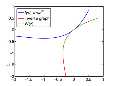
The proximity operator of $g^{*}$ at point $p$ reads (as $g^{*}$ is convex, the $\operatorname{Prox}$ operator is univalued):

$$\begin{split}\operatorname{Prox}_{\tau g^{*}}(p)&=q^{\star}\in\underset{q}{\operatorname{argmin}}\;\tfrac{1}{2\tau}|\!|q-p|\!|^{2}+g^{*}(q)\\ &=\underset{q}{\operatorname{argmin}}\;\sum_{k}\tfrac{1}{2\tau}{(q_{k}-p_{k})}^{2}+\tfrac{N}{\lambda}e^{\lambda(q_{k}-c_{k})-1}.\end{split}$$

This problem is separable and can be solved independently $\forall\,k$. Deriving the previous relation with respect to $q_{k}$, the first order optimality condition gives:

$$\begin{split}&q^{\star}_{k}-p_{k}+\tau Ne^{\lambda(q^{\star}_{k}-c_{k})-1}=0\\ \Leftrightarrow&(p_{k}-q_{k}^{*})e^{-\lambda q^{\star}_{k}}=\tau Ne^{-\lambda c_{k}-1}\\ \Leftrightarrow&\lambda(p_{k}-q_{k}^{*})e^{\lambda(p_{k}-q_{k}^{*})}=\lambda\tau Ne^{\lambda(p_{k}-c_{k})-1}.\end{split}$$

Using Lambert function, we get:

$$\begin{split}&\lambda(p_{k}-q^{\star}_{k})=W(\lambda\tau Ne^{\lambda(p_{k}-c_{k})-1})\\ \Leftrightarrow&q_{k}^{*}=p_{k}-\frac{1}{\lambda}W(\lambda\tau Ne^{\lambda(p_{k}-c_{k})-1}).\end{split}$$

The proximity operator of $g^{*}/\tau$ thus reads

$$\text{prox}_{g^{*}/\tau}(p)=p-\frac{1}{\lambda}W\left(\tfrac{\lambda}{\tau}Ne^{\lambda(p-c)-1}\right),$$

hence

$$\text{prox}_{\tau g}(p)=\frac{\tau}{\lambda}W\left(\tfrac{\lambda}{\tau}Ne^{\lambda(\tfrac{p}{\tau}-c)-1}\right).$$

∎

References

- [1] G. Aubert, M. Barlaud, O. Faugeras, and S. Jehan-Besson. Image segmentation using active contours: Calculus of variations or shape gradients? SIAM Applied Mathematics, 63(6):2128–2154, 2003.
- [2] G. Aubert and P. Kornprobst. Mathematical Problems in Image Processing, volume 147 of Applied Mathematical Sciences. Springer US, 2002.
- [3] J.-F. Aujol, G. Aubert, and L. Blanc-Féraud. Wavelet-based level set evolution for classification of textured images. IEEE Transactions on Image Processing, 12(12):1634–1641, 2003.
- [4] I. Ayed, H. Chen, K. Punithakumar, I. Ross, and S. Li. Graph cut segmentation with a global constraint: Recovering region distribution via a bound of the bhattacharyya measure. In IEEE International Conference on Computer Vision and Pattern Recognition (CVPR’10), pages 3288–3295, 2010.
- [5] B. Berkels. An unconstrained multiphase thresholding approach for image segmentation. In Scale Space and Variational Methods in Computer Vision (SSVM’09), volume 5567, pages 26–37, 2009.
- [6] N. Bonneel, J. Rabin, G. Peyré, and H. Pfister. Sliced and radon wasserstein barycenters of measures. Journal of Mathematical Imaging and Vision, 51(1):22–45, Jan. 2015.
- [7] N. Bonneel, M. van de Panne, S. Paris, and W. Heidrich. Displacement interpolation using Lagrangian mass transport. ACM Transactions on Graphics (SIGGRAPH Asia’11), 30(6), 2011.
- [8] E. Brown, T. F. Chan, and X. Bresson. Completely convex formulation of the Chan-Vese image segmentation model. International Journal of Computer Vision, 98(1):103–121, 2012.
- [9] T. Brox, M. Rousson, R. Deriche, and J. Weickert. Unsupervised segmentation incorporating colour, texture, and motion. In Computer Analysis of Images and Patterns, volume 2756, pages 353–360, 2003.
- [10] T. Brox and J. Weickert. Level set segmentation with multiple regions. IEEE Transactions on Image Processing, 15(10):3213–3218, 2006.
- [11] C. Brune. 4D imaging in tomography and optical nanoscopy. PhD thesis, University of Münster, Germany, 2010.
- [12] A. Chambolle. An algorithm for mean curvature motion. Interfaces and Free Boundaries. Mathematical Modelling, Analysis and Computation, 6(2):195–218, 2004.
- [13] A. Chambolle. An algorithm for total variation minimization and applications. Journal of Mathematical Imaging and Vision, 20(1):89–97, 2004.
- [14] A. Chambolle and J. Darbon. On total variation minimization and surface evolution using parametric maximum flows. International Journal of Computer Vision, 84(3):288–307, 2009.
- [15] A. Chambolle and T. Pock. A first-order primal-dual algorithm for convex problems with applications to imaging. Journal of Mathematical Imaging and Vision, 40:120–145, 2011.
- [16] A. Chambolle and T. Pock. On the ergodic convergence rates of a first-order primal–dual algorithm. Mathematical Programming, pages 1–35, 2015.
- [17] T. F. Chan and L. A. Vese. Active contours without edges. IEEE Transactions on Image Processing, 10(2):266–277, 2001.
- [18] L. Chizat, B. Schmitzer, G. Peyré, and F.-X. Vialard. Unbalanced Optimal Transport: Geometry and Kantorovich Formulation. Preprint arXiv: 1508.05216, 2015.
- [19] P. Combettes, L. Condat, J.-C. Pesquet, and B. Vu. A forward-backward view of some primal-dual optimization methods in image recovery. In IEEE International Conference on Image Processing (ICIP’14), pages 4141–4145, Oct 2014.
- [20] L. Condat. Fast projection onto the simplex and the l1 ball. Mathematical Programming, 158(1):575–585, 2016.
- [21] R. Corless, G. Gonnet, D. Hare, D. Jeffrey, and D. Knuth. On the lambert W function. Advances in Computational Mathematics, 5(1):329–359, 1996.
- [22] D. Cremers, M. Rousson, and R. Deriche. A review of statistical approaches to level set segmentation: Integrating color, texture, motion and shape. International Journal of Computer Vision, 72(2):215, 2007.
- [23] M. Cuturi. Sinkhorn distances: Lightspeed computation of optimal transport. In Neural Information Processing Systems (NIPS’13), pages 2292–2300, 2013.
- [24] M. Cuturi and A. Doucet. Fast computation of wasserstein barycenters. In International Conference on Machine Learning (ICML’14), pages 685–693, 2014.
- [25] M. Cuturi and G. Peyré. A smoothed dual approach for variational wasserstein problems. SIAM Journal on Imaging Sciences, 9(1):320–343, 2016.
- [26] J. Delon. Movie and video scale-time equalization application to flicker reduction. IEEE Transactions on Image Processing, 15(1):241–248, 2006.
- [27] J. Digne, D. Cohen-Steiner, P. Alliez, F. de Goes, and M. Desbrun. Feature-preserving surface reconstruction and simplification from defect-laden point sets. Journal of Mathematical Imaging and Vision, 48(2):369–382, 2014.
- [28] S. Ferradans, N. Papadakis, G. Peyré, and J.-F. Aujol. Regularized discrete optimal transport. SIAM Journal on Imaging Sciences, 7(3):1853–1882, 2014.
- [29] C. Frogner, C. Zhang, H. Mobahi, M. Araya-Polo, and T. Poggio. Learning with a wasserstein loss. Preprint arXiv: 1506.05439, 2015.
- [30] L. Gorelick, F. R. Schmidt, Y. Boykov, A. Delong, and A. Ward. Segmentation with non-linear regional constraints via line-search cuts. In European Conference on Computer Vision (ECCV’12), pages 583–597, 2012.
- [31] A. Gramfort, G. Peyré, and M. Cuturi. Fast Optimal Transport Averaging of Neuroimaging Data. In Information Processing in Medical Imaging (IPMI’15), 2015.
- [32] S. Haker, L. Zhu, A. Tannenbaum, and S. Angenent. Optimal mass transport for registration and warping. International Journal of Computer Vision, 60(3):225–240, 2004.
- [33] A. Herbulot, S. Jehan-Besson, S. Duffner, M. Barlaud, and G. Aubert. Segmentation of vectorial image features using shape gradients and information measures. Journal of Mathematical Imaging and Vision, 25(3):365–386, 2006.
- [34] D. Hochbaum and V. Singh. An efficient algorithm for co-segmentation. In International Conference on Computer Vision (ICCV’09), pages 269–276, 2009.
- [35] A. Joulin, F. Bach, and J. Ponce. Discriminative clustering for image co-segmentation. In IEEE International Conference on Computer Vision and Pattern Recognition (CVPR’10), pages 1943–1950, 2010.
- [36] M. Jung, G. Peyré, and L. D. Cohen. Texture segmentation via non-local non-parametric active contours. In Energy Minimization Methods in Computer Vision and Pattern Recognition (EMMCVPR’11), pages 74–88, 2011.
- [37] J. Kim, J. W. Fisher, A. Yezzi, M. Cetin, and A. S. Willsky. A nonparametric statistical method for image segmentation using information theory and curve evolution. IEEE Transactions on Image Processing, 14(10):1486–1502, 2005.
- [38] J. Lellmann, J. Kappes, J. Yuan, F. Becker, and C. Schnörr. Convex multi-class image labeling by simplex-constrained total variation. In Scale Space and Variational Methods in Computer Vision (SSVM’09), pages 150–162, 2009.
- [39] J. Lellmann, D. A. Lorenz, C. Schönlieb, and T. Valkonen. Imaging with kantorovich–rubinstein discrepancy. SIAM Journal on Imaging Sciences, 7(4):2833–2859, 2014.
- [40] D. Lombardi and E. Maitre. Eulerian models and algorithms for unbalanced optimal transport. ESAIM: Mathematical Modelling and Numerical Analysis, 49(3):1717 – 1744, 2015.
- [41] D. Lorenz and T. Pock. An inertial forward-backward algorithm for monotone inclusions. Journal of Mathematical Imaging and Vision, 51(2):311–325, 2015.
- [42] C. Mendoza, J.-A. Perez-Carrasco, A. Saez, B. Acha, and C. Serrano. Linearized multidimensional earth-mover’s-distance gradient flows. IEEE Transactions on Image Processing, 22(12):5322–5335, 2013.
- [43] L. Mukherjee, V. Singh, and C. R. Dyer. Half-integrality based algorithms for cosegmentation of images. In IEEE International Conference on Computer Vision and Pattern Recognition (CVPR’09), pages 2028–2035, June 2009.
- [44] D. Mumford and J. Shah. Optimal approximation by piecewise smooth functions and associated variational problems. Communications on Pure and Applied Mathematics, 42:577–685, 1989.
- [45] K. Ni, X. Bresson, T. Chan, and S. Esedoglu. Local histogram based segmentation using the wasserstein distance. International Journal of Computer Vision, 84(1):97–111, 2009.
- [46] M. Nikolova, S. Esedoglu, and T. F. Chan. Algorithms for finding global minimizers of image segmentation and denoising models. SIAM Journal on Applied Mathematics, 66(5):1632–1648, 2006.
- [47] S. Osher and J. A. Sethian. Fronts propagating with curvature-dependent speed: Algorithms based on hamilton-jacobi formulations. Journal of Computational Physics, 79(1):12–49, 1988.
- [48] N. Papadakis, E. Provenzi, and V. Caselles. A variational model for histogram transfer of color images. IEEE Transactions on Image Processing, 20(6):1682–1695, 2011.
- [49] N. Papadakis, R. Yıldızoglu, J.-F. Aujol, and V. Caselles. High-dimension multi-label problems: convex or non convex relaxation? SIAM Journal on Imaging Sciences, 6(4):2603–2639, 2013.
- [50] O. Pele and M. Werman. Fast and robust earth mover’s distances. In IEEE International Conference on Computer Vision (ICCV’09), pages 460–467, 2009.
- [51] G. Peyré, J. Fadili, and J. Rabin. Wasserstein active contours. In IEEE International Conference on Image Processing (ICIP’12), 2012.
- [52] F. Pitié, A. C. Kokaram, and R. Dahyot. Automated colour grading using colour distribution transfer. Computer Vision and Image Understanding, 107:123–137, 2007.
- [53] T. Pock, A. Chambolle, D. Cremers, and H. Bischof. A convex relaxation approach for computing minimal partitions. In IEEE Conference on Computer Vision and Pattern Recognition (CVPR’09), pages 810 –817, 2009.
- [54] T. Pock, D. Cremers, H. Bischof, and A. Chambolle. Global solutions of variational models with convex regularization. SIAM Journal of Imaging Sciences, 3(4):1122–1145, 2010.
- [55] K. Punithakumar, J. Yuan, I. Ben Ayed, S. Li, and Y. Boykov. A convex max-flow approach to distribution-based figure-ground separation. SIAM Journal on Imaging Sciences, 5(4):1333–1354, 2012.
- [56] J. Rabin, J. Delon, and Y. Gousseau. Transportation distances on the circle. Journal of Mathematical Imaging and Vision, 41(1-2):147–167, 2011.
- [57] J. Rabin and N. Papadakis. Convex color image segmentation with optimal transport distances. In Scale Space and Variational Methods in Computer Vision (SSVM’15), pages 241–252, 2015.
- [58] J. Rabin, G. Peyré, J. Delon, and M. Bernot. Wasserstein barycenter and its application to texture mixing. In Scale Space and Variational Methods in Computer Vision (SSVM’11), pages 435–446, 2012.
- [59] F. Ranchin, A. Chambolle, and F. Dibos. Total variation minimization and graph cuts for moving objects segmentation. In Scale Space and Variational Methods in Computer Vision (SSVM’07), pages 743–753, 2007.
- [60] A. Rangarajan, A. Yuille, and E. Mjolsness. Convergence properties of the softassign quadratic assignment algorithm. Neural Computation, 11(6):1455–1474, Aug. 1999.
- [61] C. Rother, T. Minka, A. Blake, and V. Kolmogorov. Cosegmentation of image pairs by histogram matching - incorporating a global constraint into mrfs. In IEEE International Conference on Computer Vision and Pattern Recognition (CVPR’06), volume 1, pages 993–1000, June 2006.
- [62] C. Rother, T. Minka, A. Blake, and V. Kolmogorov. Cosegmentation of image pairs by histogram matching-incorporating a global constraint into MRFs. In IEEE International Conference on Computer Vision and Pattern Recognition (CVPR’06), pages 993–1000, 2006.
- [63] M. Rousson, T. Brox, and R. Deriche. Active unsupervised texture segmentation on a diffusion based feature space. In IEEE International Conference on Computer Vision and Pattern Recognition (CVPR’03), pages 699–704, 2003.
- [64] J. Rubio, J. Serrat, A. Lopez, and N. Paragios. Unsupervised co-segmentation through region matching. In IEEE International Conference on Computer Vision and Pattern Recognition (CVPR’12), pages 749–756, 2012.
- [65] Y. Rubner, C. Tomasi, and L. J. Guibas. The earth mover’s distance as a metric for image retrieval. International Journal of Computer Vision, 40(2):99–121, 2000.
- [66] B. Schmitzer. A sparse multiscale algorithm for dense optimal transport. Journal of Mathematical Imaging and Vision, pages 1–22, 2016.
- [67] B. Schmitzer and C. Schnörr. Modelling convex shape priors and matching based on the gromov-wasserstein distance. Journal of Mathematical Imaging and Vision, 46(1):143–159, 2013.
- [68] B. Schmitzer and C. Schnörr. Globally optimal joint image segmentation and shape matching based on wasserstein modes. Journal of Mathematical Imaging and Vision, 52(3):436–458, 2015.
- [69] R. Sinkhorn and P. Knopp. Concerning nonnegative matrices and doubly stochastic matrices. Pacific Journal of Mathematics, 21(2):343–348, 1967.
- [70] J. Solomon, F. de Goes, G. Peyré, M. Cuturi, A. Butscher, A. Nguyen, T. Du, and L. Guibas. Convolutional wasserstein distances: Efficient optimal transportation on geometric domains. In ACM Transactions on Graphics (SIGGRAPH’15), 2015.
- [71] P. Swoboda and C. Schnörr. Variational image segmentation and cosegmentation with the wasserstein distance. In Energy Minimization Methods in Computer Vision and Pattern Recognition (EMMCVPR’13), pages 321–334, 2013.
- [72] L. A. Vese and T. F. Chan. A multiphase level set framework for image segmentation using the mumford and shah model. International Journal of Computer Vision, 50(3):271–293, 2002.
- [73] S. Vicente, V. Kolmogorov, and C. Rother. Joint optimization of segmentation and appearance models. In IEEE International Conference on Computer Vision (ICCV’09), pages 755–762, 2009.
- [74] S. Vicente, V. Kolmogorov, and C. Rother. Cosegmentation revisited: Models and optimization. In European Conference on Computer Visio (ECCV’10), pages 465–479, 2010.
- [75] S. Vicente, C. Rother, and V. Kolmogorov. Object cosegmentation. In IEEE International Conference on Computer Vision and Pattern Recognition (CVPR’11), pages 2217–2224, June 2011.
- [76] C. Villani. Topics in Optimal Transportation. AMS, 2003.
- [77] B. C. Vu. A splitting algorithm for dual monotone inclusions involving cocoercive operators. Advances in Computational Mathematics, 38(3):667–681, 2013.
- [78] R. Yıldızoğlu, J.-F. Aujol, and N. Papadakis. Active contours without level sets. In IEEE International Conference on Image Processing (ICIP’12), pages 2549–2552, 2012.
- [79] R. Yıldızoglu, J.-F. Aujol, and N. Papadakis. A convex formulation for global histogram based binary segmentation. In Energy Minimization Methods in Computer Vision and Pattern Recognition (EMMCVPR’13), pages 335–349, 2013.
- [80] Y. Yuan, E. Ukwatta, X. Tai, A. Fenster, and C. Schnörr. A fast global optimization-based approach to evolving contours with generic shape prior. UCLA Tech. Report CAM, 12-38, 2012.
- [81] C. Zach, D. Gallup, J. Frahm, and M. Niethammer. Fast global labeling for real-time stereo using multiple plane sweeps. In International Workshop on Vision, Modeling, and Visualization (VMV’08), pages 243–252, 2008.
- [82] S. Zhu, T. Lee, and A. Yuille. Region competition: unifying snakes, region growing, energy/bayes/mdl for multi-band image segmentation. In IEEE International Conference on Computer Vision (ICCV’95), pages 416 –423, 1995.