On the numerical study of percolation and epidemic critical properties in networks

Abstract

The static properties of the fundamental model for epidemics of diseases allowing immunity (susceptible-infected-removed model) are known to be derivable by an exact mapping to bond percolation. Yet when performing numerical simulations of these dynamics in a network a number of subtleties must be taken into account in order to correctly estimate the transition point and the associated critical properties. We expose these subtleties and identify the different quantities which play the role of criticality detector in the two dynamics.

1 Introduction

Epidemic processes on complex heterogeneous topologies, such as those representing social contact networks Jackson2010 , can exhibit surprising features when compared with regular or fully mixed substrates Pastor-Satorras:2014aa . Particular among those hallmarks is a vanishing epidemic threshold pv01a ; Castellano2010 , which makes heterogeneous networks exceedingly prone to the spreading of an infection, even in the case of a very small infective power. A cornerstone model for the understanding of diseases that confer immunity is the susceptible-infected-removed (SIR) model Diekmann_Heesterbeek_Britton_boek2012 . In this model, the nodes in the network (individuals) can be in three different states: susceptible ($S$), i.e. able to contract the disease; infected ($I$), i.e. able to propagate the disease to a nearest neighbor contact; and removed ($R$), immune to the disease. The dynamics of the model is as follows: each infected node connected to a susceptible node can propagate the disease to the latter with a rate (probability per unit time) $\lambda$; on the other hand, each infected individual recovers and becomes removed with a rate $\mu$ (which, without loss of generality, we fix to $\mu=1$). Notice that the total rate of infection of neighbours of a node is proportional to the number of susceptible ones. The behavior of the SIR model is characterized in terms of the statistical properties of the epidemic outbreaks it generates, measured by the average number of removed individuals $N_{R}$ at the end of an outbreak. In this sense, it is important to discern the existence of an epidemic threshold $\lambda_{c}$, separating a phase $\lambda\leq\lambda_{c}$ in which the total number of affected individuals is sublinear with the network size $N$, with $N_{R}/N\to 0$ for $N\to\infty$, from a phase $\lambda>\lambda_{c}$ in which the disease affects a finite fraction of the population, $N_{R}/N\to\mathrm{const.}>0$ for $N\to\infty$.

The properties of the SIR model have been analytically studied applying different approaches Pastor-Satorras:2014aa . In particular the so-called heterogeneous mean-field theory (HMF) refId0 ; lloyd01 ; marianproc focuses on the dynamic properties of nodes grouped in classes with the same degree and assumes an annealed network approximation dorogovtsev07:_critic_phenom , neglecting the actual network structure and considering only an ensemble of random networks, all sharing some statistical properties (degree distribution, degree correlations) Boguna09 . An alternative, more accurate, approach is based on a mapping of SIR outbreaks to a bond percolation process in the network, with a percolation probability depending on the rate of infection and recovery of the SIR process newman02 ; Pastor-Satorras:2014aa . Both approaches predict the presence of an epidemic threshold that, in degree uncorrelated networks Dorogovtsev:2002 , is a function of the first $\left\langle{k}\right\rangle$ and second $\left\langle{k^{2}}\right\rangle$ moment of the network’s degree distribution.

Despite the strength of these theoretical predictions the use of numerical techniques is still important, for both percolation and SIR on networks, since the theoretical approaches are based on the omission of topological and dynamical correlations Dorogovtsev:2002 . Most computational efforts devoted to determine the position of the critical point in either SIR or percolation Lagorio2009755 ; Colomer-de-Simon2014 ; PhysRevE.91.010801 ; Shu15 rely on some form of numerical “susceptibility”, defined in terms of moments of the cluster or outbreak sizes. These susceptibilities are designed to behave as “criticality detectors”, in the sense that they should exhibit a peak in the vicinity of the critical point, and decrease sensibly away from it. The variation of the position and height of the peak as a function of the network size is then used to determine the position of the critical point in the thermodynamic (infinite network) limit, as well as the associated critical exponents, by applying finite-size scaling (FSS) theory cardy88 . While the susceptibilities used so far in the literature usually work numerically, there has not been, to the best of our knowledge, any effort to put them on a sound theoretical footing, in particular, in what refers to the differences in the susceptibilities used for percolation and the SIR model, and in the relation with the mapping from one process to the other.

The purpose of this paper is to undertake this effort, by examining critically the different numerical methods applied so far to determine the critical properties of the bond percolation and the SIR transitions. We find that, despite the exact mapping existing between the two models, different quantities must be considered in the numerical study of the two cases. Moreover, particular care must be used in the evaluation of the critical properties of SIR and its comparison with theoretical predictions.

The paper is structured as follows. In Sec. 2 we briefly summarize the results for percolation and SIR that will be needed in the rest of the paper. In Sec. 3 we define different quantities that may be detectors of criticality for percolation processes on networks, we determine analytically and verify numerically which one is the most suitable. We then adapt the same framework to the SIR model, highlighting the differences between the two cases, which result in different quantities being optimal detectors of criticality. A discussion of the implications of our findings and a reinterpretation of previous literature, followed by conclusions is presented in Sec. 4.

2 Background on percolation and the SIR model

In this section we briefly summarize standard results on percolation and the SIR model that will be needed in the rest of the paper.

2.1 Percolation in lattices

In bond percolation, edges are removed with probability $1-p$ and kept with probability $p$. In regular Euclidean lattices stauffer94 , a critical value $p_{c}$ separates a subcritical phase at $p\leq p_{c}$ in which only small clusters of connected sites exist, from a supercritical phase at $p>p_{c}$, where there is an infinite, spanning cluster. In finite Euclidean systems, the spanning cluster is defined as any cluster that touches two opposite boundaries along a given coordinate axis. The order parameter is thus defined as the probability $\mathcal{P}$ (the percolation strength) that a randomly selected site belongs to the spanning cluster. In an infinite system, above the transition

$$\mathcal{P}\sim(p-p_{c})^{\beta},$$ (1)

defining the critical exponent $\beta$. The principal quantity in percolation, from which all others can be derived, is the normalized cluster number, $n_{s}(p)$, defined as the number of finite clusters of size $s$ per lattice site. A consequence of this definition is that $sn_{s}(p)/\sum_{s^{\prime}}s^{\prime}n_{s^{\prime}}(p)$ is the probability that a randomly chosen site belongs to a finite cluster of size $s$ stauffer94 . In order to determine numerically both the critical point and the associated critical exponents, one usually studies the so-called mean cluster size (or susceptibility) stauffer94 ,

$$\chi=\sum_{s}s\frac{sn_{s}(p)}{\sum_{s^{\prime}}s^{\prime}n_{s^{\prime}}(p)}.$$ (2)

The susceptibility $\chi$ assumes, in an infinite lattice, a finite value for any $p$ except at the critical point, $p_{c}$, where it diverges as

$$\chi\sim|p-p_{c}|^{-\gamma}$$ (3)

This divergence is related to the scaling form of the normalized cluster number, which, close to the critical point, obeys

$$n_{s}(p)\simeq s^{-\tau}{\cal F}(s\Delta^{1/\sigma}),$$ (4)

with $\Delta=|p-p_{c}|$, $\cal{F}$ is a scaling function, while $\tau$ and $\sigma$ are other critical exponents, related to $\beta$ and $\gamma$ through the relations stauffer94

$$\sigma=\frac{1}{\beta+\gamma},\quad\tau=3-\frac{\gamma}{\beta+\gamma}.$$ (5)

Right at the critical point, we can apply FSS theory stauffer94 ; cardy88 to see how quantities depend on system size in finite systems. The basic FSS hypothesis states that the system size dependence enters in the system by the ratio $\xi/L$, where $L$ is the longitudinal length and $\xi\sim\Delta^{-\nu}$ the correlation length stauffer94 . Thus, assuming that the order parameter follows, close to criticality, the scaling form

$$\mathcal{P}(p,L)=L^{-\beta/\nu}F(\Delta^{\nu}L)$$ (6)

we are led to susceptibility scaling at the critical point as

$$\chi(p_{c})\simeq L^{\gamma/\nu},$$ (7)

while the order parameter scales as

$$\mathcal{P}(p_{c})\simeq L^{-\beta/\nu}.$$ (8)

Notice that these last expressions can be simply obtained by replacing $\Delta\sim L^{-1/\nu}$ in Eqs. (1) and (3).

2.2 Percolation in networks

In networks all definitions presented above can be used, with only one caveat: Since there is no network boundary, it is not possible to define a spanning cluster, and hence one has to use alternative definitions of the order parameter $\mathcal{P}$. The natural modification involves the consideration of the largest component of the network, which has size $S$. In the limit of infinite network, below the critical point the size of the largest component is subextensive: $S/N\to 0$; above the critical point, on the other hand, the largest component is the giant connected component of the network Newman10 , with a size $S\equiv G\sim N$, proportional to the network size. In this way, we can define the percolation strength as $\mathcal{P}=G/N$, which is finite above the critical point.

For random uncorrelated networks the condition for the existence of the giant component is Callaway2000

$$p>p_{c}=\frac{\left\langle{k}\right\rangle}{\left\langle{k^{2}}\right\rangle-\left\langle{k}\right\rangle}.$$ (9)

The behavior of the order parameter close to criticality is ${\cal P}\sim(p-p_{c})^{\beta}$, where the critical exponent $\beta$ depends on the form of the degree distribution. For scale-free networks with a degree distribution $P(k)\sim k^{-\gamma_{d}}$, one finds Cohen02

$$\beta=\left\{\begin{array}[]{ccc}1/(3-\gamma_{d})&\mathrm{for}&2<\gamma_{d}<3\\ 1/(\gamma_{d}-3)&\mathrm{for}&3<\gamma_{d}<4\\ 1&\mathrm{for}&\gamma_{d}>4\end{array}\right..$$ (10)

Applying the FSS theory, and assuming a scaling of the order parameter, following Eq. (6), in the form

$$\mathcal{P}(p,N)=N^{-\beta/\nu}F(\Delta^{\nu}N),$$ (11)

one finds Radicchi15 ; Wu07

$$\nu=\left\{\begin{array}[]{ccc}2/(3-\gamma_{d})&\mathrm{for}&2<\gamma_{d}<3\\ (\gamma_{d}-1)/(\gamma_{d}-3)&\mathrm{for}&3<\gamma_{d}<4\\ 3&\mathrm{for}&\gamma_{d}>4\end{array}\right..$$ (12)

Notice that $\nu$ describes the scaling with respect to the network size and, for the case $2<\gamma_{d}<3$, one assumes a maximum degree in the network scaling as $k_{\mathrm{max}}\sim N^{1/2}$ mariancutofss . For any $\gamma_{d}>3$ Cohen02 , it holds

$$\gamma=1,$$ (13)

while for $2<\gamma_{d}<3$ the exponent $\gamma$ is effectively 0 Radicchi15 .

2.3 Mapping SIR to percolation

The possibility of studying the SIR model by mapping it to a percolation process was observed as early as in Refs. Ludwig1975 ; Grassberger1983 . In networks, the mapping is worked out as follows newman02 . Let us consider a modified SIR model, in which infected nodes remain in this state for a fixed time $\tau$ after infection. Consider now an infected node and an edge joining it to a susceptible node. During the infection time $\tau$, since the transmission of the disease along the edge follows a Poisson process with rate $\lambda$, the probability that the infection will be transmitted along the edge is given by the transmissibility $T_{\tau}$, which takes the value renewal

$$T_{\tau}=1-e^{-\lambda\tau}.$$ (14)

As this transmissibility is the same for all infected nodes and edges, it is clear that the set of removed nodes generated by a SIR outbreak starting from a single infected node will be equal to the connected cluster the initial infected node belongs to in a bond percolation process with occupation probability $p=T_{\tau}$. From this mapping, the presence of a critical occupation probability $p_{c}$ implies the existence of a critical transmissibility $T_{\tau,c}$, which translates into a critical spreading rate $\lambda_{c}$. For uncorrelated networks, Eq. (9) for $p_{c}$ implies, using Eq. (14),

$$\lambda_{c}=\frac{1}{\tau}\ln\frac{\left\langle{k^{2}}\right\rangle-\left\langle{k}\right\rangle}{\left\langle{k^{2}}\right\rangle-2\left\langle{k}\right\rangle}.$$ (15)

The previous expression was derived assuming a constant infection time $\tau$. In general, the original definition of the SIR model, in terms of a constant recovery rate $\mu$, implies that recovery is a Poisson process, with a distribution of recovery times $P_{\mathrm{rec}}(\tau)=\mu e^{-\tau\mu}$ renewal . One possibility to deal with this fact is to consider the average transmissibility

$$\left\langle{T}\right\rangle=\int_{0}^{\infty}T_{\tau}P_{\mathrm{rec}}(\tau)\;d\tau=\frac{\lambda}{1+\lambda},$$ (16)

where we have set $\mu=1$ newman02 . The averaging performed in Eq. (16) is in principle an approximation, which nevertheless leads to exact results for the threshold Kenah2007 ; Pastor-Satorras:2014aa . In the case of uncorrelated networks, using Eq. (9), the exact threshold is

$$\lambda_{c}=\frac{\left\langle{k}\right\rangle}{\left\langle{k^{2}}\right\rangle-2\left\langle{k}\right\rangle}.$$ (17)

3 Numerical analysis of percolation and the SIR model on networks

3.1 Percolation

From a numerical point of view, the identification of the percolation critical point in regular lattices can be performed by applying the FSS hypothesis to the susceptibility $\chi$. Thus, assuming the analogous scaling form stauffer94

$$\chi(p,L)\simeq L^{\gamma/\nu}F(\Delta^{\nu}L)$$ (18)

we are led in finite systems to the presence of a peak in $\chi(p,L)$, located at $p_{c}(L)$ shifted from the infinite size critical point as

$$|p_{c}(L)-p_{c}|\sim L^{-1/\nu}.$$ (19)

The value of the susceptibility at this peak scales as

$$\chi(p_{c}(L))\sim L^{\gamma/\nu},$$ (20)

while the order parameter scales as

$$\mathcal{P}(p_{c}(L))\simeq L^{-\beta/\nu}.$$ (21)

In the case of networks, the application of this procedure is hindered by the impossibility of defining a cluster to be spanning, and thus distinguishing between percolating and finite clusters. A different approach is thus often followed Colomer-de-Simon2014 based on the fluctuations of the order parameter. We analyze here this approach, which can be applied to study also the SIR model, [while the one based on $\chi$ (Eq. (2)) obviously cannot, because for SIR only one cluster per run is generated]. Let us define the order parameter

$$\phi=\frac{S}{N}$$ (22)

where $S$ is the size of the largest cluster. In the limit $N\to\infty$, for $p\leq p_{c}$, there is no giant component and $S$ is the size of a finite component, so that $\phi\to 0$. For $p>p_{c}$ instead, $S=G$, and thus $\phi=\mathcal{P}$ is finite.

From this quantity and its moments, different definitions of susceptibility, aiming at determining the critical point and associated critical exponents, can be considered:

• Standard susceptibility in non-equilibrium phase transitions Marrobook

  $$\chi_{1}=N[\left\langle{\phi^{2}}\right\rangle-\left\langle{\phi}\right\rangle^{2}]=\frac{\left\langle{S^{2}}\right\rangle-\left\langle{S}\right\rangle^{2}}{N}$$ (23)

• Susceptibility proposed for epidemic processes in networks Ferreira12 ; Colomer-de-Simon2014 ; PhysRevE.91.010801

  $$\chi_{2}=N\frac{\left\langle{\phi^{2}}\right\rangle-\left\langle{\phi}\right\rangle^{2}}{\left\langle{\phi}\right\rangle}=\frac{\left\langle{S^{2}}\right\rangle-\left\langle{S}\right\rangle^{2}}{\left\langle{S}\right\rangle}$$ (24)

• Epidemic variability Crapey2006 ; Shu15

  $$\chi_{3}^{\prime}=\frac{\sqrt{\left\langle{\phi^{2}}\right\rangle-\left\langle{\phi}\right\rangle^{2}}}{\left\langle{\phi}\right\rangle}=\sqrt{\frac{\left\langle{S^{2}}\right\rangle}{\left\langle{S}\right\rangle^{2}}-1}$$ (25)

  Inspired by this definition, we will consider here the simplified form

  $$\chi_{3}=\frac{\left\langle{\phi^{2}}\right\rangle}{\left\langle{\phi}\right\rangle^{2}}=\frac{\left\langle{S^{2}}\right\rangle}{\left\langle{S}\right\rangle^{2}}.$$ (26)

In all previous definitions brackets $\langle\cdot\rangle$ indicate averaging over different realizations of the percolation process. We now analyze the suitability of each of these quantities as detectors of criticality, by checking whether they fulfill the requirement that they show a maximum close to the critical point, whose position tends to $p_{c}$ while the height diverges as the system size $N$ grows.

All three susceptibilities defined above ($\chi_{1},\chi_{2},\chi_{3}$) tend to a finite value for all values of $p>p_{c}$ as the system size diverges, because $\left\langle{S}\right\rangle\sim N$, $\left\langle{S^{2}}\right\rangle\sim N^{2}$ and the fluctuations are Gaussian $\left\langle{S^{2}}\right\rangle-\left\langle{S}\right\rangle^{2}\sim N$. In the opposite limit $p\to 0$, considering $p$ of the order of $N^{-1}$, we have that all moments $\left\langle{S^{k}}\right\rangle$ are independent of $N$ (since essentially the number of edges added does not depend on $N$), so that $\chi_{2}$ and $\chi_{3}$ go to a constant for $p\to 0$, while $\chi_{1}$ goes to zero.

Let us now analyze the behavior at the critical point for large $N$. At criticality, the largest component in Euclidean lattices coincides with the incipient spanning cluster $G_{i}$ stauffer94 , that is, the spanning cluster observed at the percolation threshold, whose size scales as a power of the system size, $\left\langle{G_{i}}\right\rangle\sim L^{d-\beta/\nu}$. In Ref. Coniglio1980 , it is proven that, in a regular $d$-dimensional lattice of size $L$ ($N=L^{d}$) one has

$$\frac{\left\langle{G_{i}^{2}}\right\rangle-\left\langle{G_{i}}\right\rangle^{2}}{N}\sim\frac{\left\langle{G_{i}^{2}}\right\rangle}{N}\sim\frac{\left\langle{G_{i}}\right\rangle^{2}}{N}\sim L^{\gamma/\nu},\;\frac{\left\langle{G_{i}}\right\rangle}{N}\sim L^{-\beta/\nu}.$$ (27)

Assuming that the same scaling laws can be extended to the behavior of the largest cluster size $S_{c}$ at the percolation threshold in networks, with the system size $L$ replaced by the network size $N$, we have

$$\frac{\left\langle{S_{c}^{2}}\right\rangle-\left\langle{S_{c}}\right\rangle^{2}}{N}\sim\frac{\left\langle{S_{c}^{2}}\right\rangle}{N}\sim\frac{\left\langle{S_{c}}\right\rangle^{2}}{N}\sim N^{\gamma/\nu},\quad\frac{\left\langle{S_{c}}\right\rangle}{N}\sim N^{-\beta/\nu},$$ (28)

with the corresponding change in the definition of the exponent $\nu$. As we will see below, the previous scaling forms are confirmed by percolation simulations in random networks. The scaling relations in Eq. (28) can be also obtained by assuming the so-called first scaling law 1742-6596-297-1-012005 for the probability distribution of the order parameter at criticality

$$P(S_{c})=\frac{1}{\left\langle{S_{c}}\right\rangle}F(S_{c}/\left\langle{S_{c}}\right\rangle),$$ (29)

which implies

$$\left\langle{S_{c}^{k}}\right\rangle\sim\left\langle{S_{c}}\right\rangle^{k}.$$ (30)

This leads to the results in Eq. (28), assuming $\left\langle{S_{c}}\right\rangle/N\simeq N^{-\beta/\nu}$ and the hyperscaling relation

$$\frac{2\beta}{\nu}+\frac{\gamma}{\nu}=1.$$ (31)

Inserting Eqs. (28) into the definitions of the susceptibilities we obtain the behavior at criticality

$$\chi_{1}(p_{c})\sim N^{\gamma/\nu},\quad\chi_{2}(p_{c})\sim N^{(\gamma+\beta)/\nu},\quad\chi_{3}(p_{c})\sim\mathrm{const}.$$ (32)

The previous relationships show that $\chi_{1}$ and $\chi_{2}$ are suitable criticality detectors: They diverge at the critical point, while tending to a constant value away from criticality. In this respect, $\chi_{2}$ should be numerically preferred, as it diverges with a larger exponent. The susceptibility $\chi_{3}$ instead does not depend on $N$ at criticality. This makes it rather unsuitable as criticality detector in the usual sense of a susceptibility with a diverging peak; however $\chi_{3}$ might play in this case a role analogue to Binder’s cumulant for Ising-like equilibrium transitions Binder81 ; Binderbook ; Dickman98 : a function of the control parameter $p$ changing with the system size $N$ for all values of $p$ except $p_{c}$, so that the latter is the estimated as the value where curves of $\chi_{3}(p)$, computed for different of $N$, intersect each other.

We have checked the performance of these three different criticality detectors by performing bond percolation experiments using the Newman-Ziff algorithm Newman2000 ; NewmanZiff2001 on two examples of networks for which exact values of the percolation point and critical exponents are available: Random regular networks and scale-free networks generated with the uncorrelated configuration model (UCM) Catanzaro05 . In random regular networks (RRN) all nodes have the same degree $K$, with edges randomly distributed among them, preventing self-connections and multiple connections. The critical point is, according to Eq. (9),

$$p_{c}=\frac{1}{K-1},$$ (33)

while the values of the associated critical exponents are, from Eqs. (10), (12), and (13), $\beta_{\mathrm{th}}=\gamma_{\mathrm{th}}=1$, and $\nu_{\mathrm{th}}=3$. In our simulations, we fix $K=5$, leading to the theoretical critical point $p_{c}^{\mathrm{RRN,th}}=0.25$. For scale-free networks, we consider a degree exponent $\gamma_{d}=3.5$, with a minimum degree $k_{\mathrm{min}}=3$ and a maximum degree $k_{\mathrm{max}}=N^{1/{(\gamma_{d}-1)}}$, equal to the so-called natural cut-off mariancutofss . In this case, the percolation threshold takes the form of Eq. (9). Considering a pure discrete power-law form $P(k)=k^{-\gamma}/\sum_{q=k_{\mathrm{min}}}^{\infty}q^{-\gamma}$, we obtain $p_{c}^{\mathrm{UCM,th}}=0.15054$. For this degree exponent, from Eqs. (10), (12), and (13), we have $\beta_{\mathrm{th}}=2$, $\gamma_{\mathrm{th}}=1$, and $\nu_{\mathrm{th}}=5$. In our simulations, the moments of the largest cluster $\left\langle{S^{k}}\right\rangle$ are computed averaging over $10000$ bond percolation realizations on fixed networks of different size.

In the first place, we proceed to verify that the scaling relations in Eqs. (28) are observed numerically for percolation on RRN networks. Thus, in Fig. 1 we plot different moments of the distribution of the largest cluster size, computed at the theoretical critical point $p_{c}^{\mathrm{RRN,th}}=0.25$.

Figure 1: Numerical check of the scaling relations in Eq. (28) on RRN with fixed degree $K=5$.

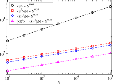
As we can see, the scaling relations assumed in Eq. (28) are perfectly satisfied, within the numerical accuracy of our simulations.

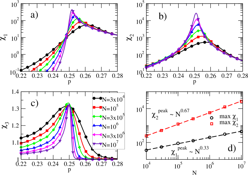
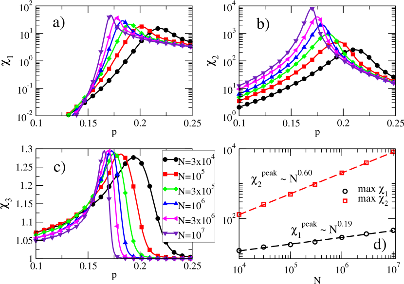
We next plot the different susceptibilites as a function of $p$ for different network sizes in the case of RRN, Fig. 2, and UCM networks, Fig. 3. As we can see, in both cases $\chi_{1}$ and $\chi_{2}$ show peaks of height increasing with $N$, located at positions $p_{c}(N)$ that change with network size, moving with increasing $N$ towards smaller $p$ values.

Figure 2: Panels (a,b,c): Different susceptibilities for bond percolation in RRN networks with degree $K=5$. Panel (d): Scaling of the height of peaks of the susceptibilities $\chi_{1}$ and $\chi_{2}$ as a function of the network size.

Figure 3: Panels (a,b,c): Different susceptibilities for bond percolation in UCM networks with degree exponent $\gamma_{d}=3.5$. Panel (d): Scaling of the height of peaks of the susceptibilities $\chi_{1}$ and $\chi_{2}$ as a function of the network size.

From the divergence of the height of the peaks of the susceptibilities we can obtain the values of exponent ratios involving $\gamma$. Indeed, assuming that the susceptibilities $\chi_{1}$ and $\chi_{2}$ obey the FSS form (see Eq. (18))

$$N^{-\alpha_{i}/\nu}\chi_{i}(p,N)=F_{i}[(p-p_{c})N^{1/\nu}],$$ (34)

where $\alpha_{1}=\gamma$ and $\alpha_{2}=\gamma+\beta$, we obtain that the height of the susceptibilities at their peak, $\chi_{i}^{\mathrm{peak}}=\chi_{i}(p_{c}(N))$, must satisfy

$$\chi_{1}^{\mathrm{peak}}\sim N^{\gamma/\nu},\quad\chi_{2}^{\mathrm{peak}}\sim N^{(\gamma+\beta)/\nu}.$$ (35)

From a linear regression in logarithmic scale of the peak height as a function of $N$, we obtain for RRN (Fig. 2(d)) the exponent ratios $\gamma/\nu=0.33(1)$, $(\beta+\gamma)/\nu=0.67(1)$, which compare very well with the theoretical values $\gamma_{\mathrm{th}}/\nu_{\mathrm{th}}=1/3$ and $(\gamma_{\mathrm{th}}+\beta_{\mathrm{th}})/\nu_{\mathrm{th}}=2/3$. For UCM networks (Fig. 3(d)) we find $\gamma/\nu=0.19(1)$, $(\gamma+\beta)/\nu=0.60(1)$, in excellent agreement with the theoretical expectations $\gamma_{\mathrm{th}}/\nu_{\mathrm{th}}=0.2$ and $(\gamma_{\mathrm{th}}+\beta_{\mathrm{th}})/\nu_{\mathrm{th}}=0.6$.

From the positions of the peaks $p_{c}(N)$ as a function of $N$ we can obtain information on the asymptotic critical point (in the infinite network size limit) and the exponent $\nu$, assuming the validity of Eq. (19). In this case, we can write

$$p_{c}(N)=p_{c}-aN^{-1/\nu},$$ (36)

where $a$ is some constant prefactor. By means of a non-linear fitting of data to Eq. (36), the values of $p_{c}$ and $\nu$ can be estimated. From such a non-linear fitting, we obtain for RRN the value $\nu=3.1(2)$ for $\chi_{1}$ and $\nu=3.2(2)$ for $\chi_{2}$, with a critical point $p_{c}=0.2498(1)$ coincident for both susceptibilities, see Fig. 4.

Figure 4: Plot of the peak position as a function of $N$ for bond percolation on RRN (a) and UCM networks with $\gamma_{d}=3.5$ (b). The linear behavior is in agreement with Eq. (36).

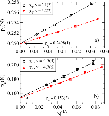
In the case of RRN networks, a single network sample is sufficient, due to the fact that the position of the peaks $p_{c}(N)$ fluctuates very slightly from sample to sample. These fluctuations are stronger in UCM networks, so we proceed to estimate the peak in 10 different samples of networks of given size $N$, and compute from them the average position $p_{c}(N)$ and associated error, see Fig. 4. Applying to this data a non-linear fitting to the form of Eq. (36), we obtain $\nu=4.5(4)$ for $\chi_{1}$ and $\nu=4.7(6)$ for $\chi_{2}$, with a common critical point $p_{c}=0.153(2)$. The values thus obtained show a very good match with the theoretical expectations for the RRN, $p_{c}^{\mathrm{RRN,th}}=0.25$ and $\nu_{\mathrm{th}}=3$, and provide a quite reasonable approximation in the case of UCM networks, $p_{c}^{\mathrm{RRN,th}}=0.15054$ and $\nu_{\mathrm{th}}=5$.

In order to check the accuracy of the different susceptibilities with respect to the known exact values of the critical point and critical exponents, we perform a data collapse analysis. The validity of FSS hypothesis above implies that plotting the values of the susceptibilities rescaled according to Eq. (34) curves for different values of $N$ will collapse onto the same universal function $F_{i}(x)$ for $x=(p-p_{c})N^{1/\nu}$, when the correct values of the critical points and critical exponents are used.

Figure 5: Data collapse analysis of the susceptibilities $\chi_{1}$ (top) and $\chi_{2}$ (bottom) for bond percolation on RRN of degree $K=5$. We have used the exact theoretical values $p_{c}^{\mathrm{RRN,th}}=0.25$, $\nu_{\mathrm{th}}=3$, $\gamma_{\mathrm{th}}/\nu_{\mathrm{th}}=1/3$, $(\beta_{\mathrm{th}}+\gamma_{\mathrm{th}})/\nu_{\mathrm{th}}=2/3$.

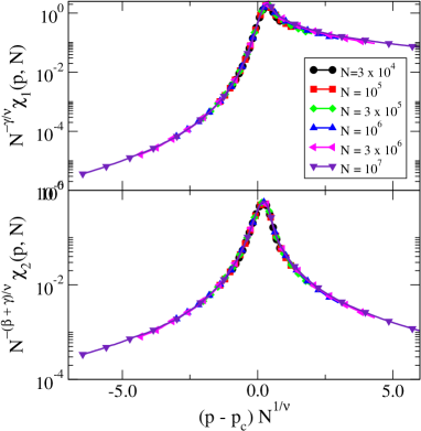
In Fig. 5 we show the data collapse analysis for the RRN. In this case, a perfect data collapse is obtained with the exact theoretical results $p_{c}^{\mathrm{RRN,th}}=0.25$, $\nu_{\mathrm{th}}=3$, $\gamma_{\mathrm{th}}/\nu_{\mathrm{th}}=1/3$, $(\beta_{\mathrm{th}}+\gamma_{\mathrm{th}})/\nu_{\mathrm{th}}=2/3$.

Figure 6: Data collapse analysis of the susceptibilities $\chi_{1}$ (top) and $\chi_{2}$ (bottom) for bond percolation on UCM of degree exponent $\gamma_{d}=3.5$. We have used the numerical critical point $p_{c}^{\mathrm{UCM}}=0.153$, and the exponents $\nu=4.7$, $\gamma/\nu=0.19$ and $(\gamma+\beta)/\nu=0.60$.

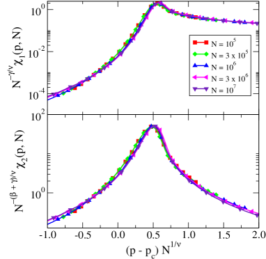
Concerning the scale-free UCM networks, a very good data collapse is obtained using the numerical parameters previously estimated from the analysis of the peak height and peak position of the susceptibilities, namely $p_{c}^{\mathrm{UCM}}=0.153$, $\gamma/\nu=0.19$, $(\gamma+\beta)/\nu=0.60$, and $\nu=4.7$.

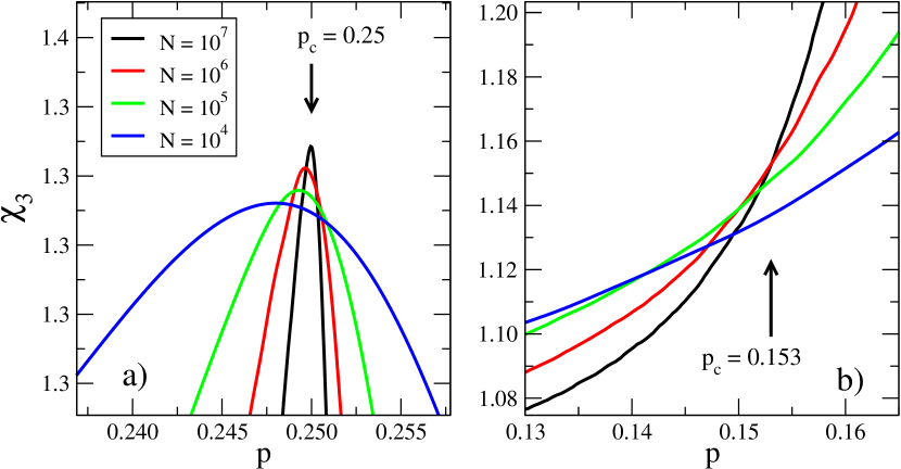
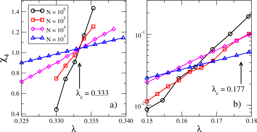
As we have pointed out above, one could think on using the constant value of the susceptibility $\chi_{3}$ as a method to determine the critical point in the sense of the Binder cumulant: Since $\chi_{3}(p_{c})$ does not depend on network size, curves of $\chi_{3}(p)$ for different values of $N$ should cross exactly at $p_{c}$, allowing thus to identify $p_{c}$. The usefulness of this method, however, is hindered by the fact that, at odds with the originally defined Binder cumulant, $\chi_{3}(p)$ has in general an asymptotic form that is not a step function Binder81 : The limits for large and small values of $p$ are very similar, and the function exhibits a peak close to $p_{c}$. In the case of RRN, see a close up in the vicinity of the critical point in Fig. 7(a), the peaks are so close to the critical point that in general two intersection points can be observed for every pair of curves, rendering them unsuitable for the determination of $p_{c}$. In the case of UCM networks with $\gamma_{d}=3.5$, Fig. 3(b), the crossing is sufficiently away from the peak to allow an estimate of the crossing point which is in reasonable agreement with the estimated numerical one, $p_{c}^{\mathrm{UCM}}\simeq 0.153$, for the largest network sizes considered, see the corresponding close up in Fig. 7(b).

Figure 7: Close up of the susceptibility $\chi_{3}$ in the vicinity of the critical point for RRN networks (a) and UCM networks with $\gamma_{d}=3.5$ (b). In this last case, we consider the average over $10$ different network samples.

3.2 SIR model

The SIR process is mapped exactly to bond percolation. However, when the two processes are simulated numerically, there is a crucial difference: In a percolation experiment, we have information on the whole cluster structure for each percolation configuration, and we can pick the largest cluster to perform statistics. On the other hand, in the SIR process, we obtain only one outbreak, corresponding to a particular percolation cluster, in every run. Therefore, averages over different outbreak sizes are the only available information. Moreover, since the seed of SIR outbreaks is chosen randomly among all vertices, epidemic outbreaks are bond percolation clusters sampled with a probability proportional to their size. In other words, when an outbreak occurs above the critical point, this corresponds to the giant component, of size $G$, with probability $P_{G}=G/N$, and to a finite cluster with probability $P_{F}=1-P_{G}$. On the other hand, when the system is below the critical point, all outbreaks correspond to finite clusters. Thus, if we define the order parameter as the relative outbreak size, $\phi=N_{R}/N$, when computing its moments in SIR simulations we are performing, in the general case, an implicit double average:

1. For a fixed percolation configuration, we are selecting the giant component with probability $P_{G}$, and finite clusters with probability $1-P_{G}$. In the latter case, a finite cluster of size $s$ is selected with probability $\sim sn_{s}$. Importantly, this first average is made at constant $G$ (the size of the giant component of the fixed percolation configuration).

   For the fixed percolation configuration, the $n$-th moment of the order parameter $\phi$ is thus

   $$\overline{\phi^{n}} = \left(\frac{G}{N}\right)^{n}P_{G}+\sum_{s<G}\left(\frac{s}{N}\right)^{n}\frac{sn_{s}}{\sum_{s^{\prime}<G}s^{\prime}n_{s^{\prime}}}P_{F}$$ (37)

   $$= \left(\frac{G}{N}\right)^{n+1}+\mu\sum_{s<G}\left(\frac{s}{N}\right)^{n}sn_{s}\left(1-\frac{G}{N}\right)$$

   where $\mu^{-1}=\sum_{s^{\prime}<G}s^{\prime}n_{s^{\prime}}$ is a normalization factor that tends to a constant in the limit of large $N$.

2. After this average, an average over different percolation configurations, described by the distribution of giant component sizes $g(G)$, must be performed. Thus we have

   $$\left\langle{\overline{\phi^{n}}}\right\rangle = \left\langle{\left(\frac{G}{N}\right)^{n+1}}\right\rangle_{g}+\mu\sum_{s<G}\left(\frac{1}{N}\right)^{n}\left\langle{s^{n+1}n_{s}\left(1-\frac{G}{N}\right)}\right\rangle_{g}$$

   $$\equiv \sum_{S}\left(\frac{G}{N}\right)^{n+1}g(G)+\mu\sum_{s<G}\left(\frac{1}{N}\right)^{n}\left\langle{s^{n+1}n_{s}\left(1-\frac{G}{N}\right)}\right\rangle_{g}$$

Assuming that the largest cluster and the finite clusters are uncorrelated ($\langle s^{n+1}G\rangle=\langle s^{n+1}\rangle\langle G\rangle$) we have

$$\left\langle{\overline{\phi^{n}}}\right\rangle=\frac{\left\langle{G^{n+1}}\right\rangle}{N^{n+1}}+\mu\frac{\left\langle{s^{n+1}}\right\rangle}{N^{n}}\left(1-\frac{\left\langle{G}\right\rangle}{N}\right)$$ (38)

where the averages $\left\langle{s^{k}}\right\rangle$ of finite clusters are performed with the probability $n_{s}(p)$.

Let us analyze the scaling of the three candidate susceptibilities at the critical point. Considering first the approach to criticality from below. Since there is no giant component, we have

$$\left\langle{\overline{\phi^{n}}}\right\rangle=\frac{\left\langle{s^{n+1}}\right\rangle}{N^{n}}.$$ (39)

Below the critical point, the moments $\left\langle{s^{k}}\right\rangle$ can be computed from the scaling ansatz for the normalized cluster number $n_{s}(p)$, see Eqs. (4) and (5), leading to

$$\left\langle{s^{2}}\right\rangle\simeq\Delta^{-\gamma},\quad\left\langle{s^{3}}\right\rangle\simeq\Delta^{-(4-\tau)/\sigma}\simeq\Delta^{-(\beta+2\gamma)}.$$ (40)

Applying the FSS hypothesis, substituting $\Delta\sim N^{-1/\nu}$, we have, at criticality,

$$\left\langle{s^{2}}\right\rangle_{c}\simeq N^{\gamma/\nu},\quad\left\langle{s^{3}}\right\rangle_{c}\simeq N^{(\beta+2\gamma)/\nu},$$ (41)

and from here

$$\left\langle{\overline{\phi}}\right\rangle_{c}\simeq N^{\gamma/\nu-1},\quad\left\langle{\overline{\phi^{2}}}\right\rangle_{c}\simeq N^{(\beta+2\gamma)/\nu-2}.$$ (42)

Therefore, we have

$$\chi_{1}(\lambda_{c})=N[\left\langle{\overline{\phi^{2}}}\right\rangle_{c}-\left\langle{\overline{\phi}}\right\rangle^{2}_{c}]\simeq N^{(\beta+2\gamma)/\nu-1}\simeq N^{(\gamma-\beta)/\nu},$$ (43)

where the hyperscaling relation Eq. (31) has been used. For $\chi_{2}(\lambda_{c})$, in the limit of large $N$, we have

$$\chi_{2}(\lambda_{c})=\frac{\chi_{1}(\lambda_{c})}{\left\langle{\overline{\phi}}\right\rangle_{c}}\simeq N^{1-\beta/\nu},$$ (44)

and, finally, for $\chi_{3}$

$$\chi_{3}(\lambda_{c})=\frac{\left\langle{\overline{\phi^{2}}}\right\rangle_{c}}{\left\langle{\overline{\phi}^{2}}\right\rangle)c}\simeq N^{\beta/\nu}.$$ (45)

Results for the same quantities can be derived when approaching criticality from above. In this case, $\left\langle{G^{k}}\right\rangle$ has the leading behavior and terms $\left\langle{s^{k}}\right\rangle$ can be disregarded. The definitions of the candidate susceptibilities become therefore

$$\chi_{1}=N[\left\langle{\overline{\phi^{2}}}\right\rangle-\left\langle{\overline{\phi}}\right\rangle^{2}]=\frac{\left\langle{G^{3}}\right\rangle-\left\langle{G^{2}}\right\rangle^{2}/N}{N^{2}}$$ (46)

$$\chi_{2}=N\frac{\left\langle{\overline{\phi^{2}}}\right\rangle-\left\langle{\overline{\phi}}\right\rangle^{2}}{\left\langle{\overline{\phi}}\right\rangle}=\frac{\left\langle{G^{3}}\right\rangle-\left\langle{G^{2}}\right\rangle^{2}/N}{\left\langle{G^{2}}\right\rangle}$$ (47)

$$\chi_{3}=\frac{\left\langle{\overline{\phi^{2}}}\right\rangle}{\left\langle{\overline{\phi}}\right\rangle^{2}}=\frac{N\left\langle{G^{3}}\right\rangle}{\left\langle{G^{2}}\right\rangle^{2}}$$ (48)

For fixed $\lambda>\lambda_{c}$ and large $N$, the numerator of $\chi_{1}$ and $\chi_{2}$ increases as $N^{3}$ so that both $\chi_{1}$ and $\chi_{2}$ grow linearly with $N$. This is already enough to declare the two quantities unsuitable as detectors of criticality. Instead it is trivial to see that $\chi_{3}$ goes to a finite limit as $N\to\infty$. Let us also check the behavior at criticality. Right at the critical point we assume that the size of the largest component obeys $\left\langle{S_{c}^{3}}\right\rangle\sim\left\langle{S_{c}^{2}}\right\rangle\left\langle{S_{c}}\right\rangle$, which follows from the scaling relation Eq. (29). Hence, from Eq. (28), $\left\langle{S_{c}^{3}}\right\rangle\sim N^{2+(\gamma-\beta)/\nu}$ so that

$$\chi_{1}(\lambda_{c})\simeq\frac{\left\langle{S_{c}^{3}}\right\rangle}{N^{2}}\sim N^{(\gamma-\beta)/\nu}$$ (49)

We conclude that this function is in general not a good detector of criticality, since in general $\gamma\leq\beta$, and therefore $\chi_{1}(\lambda_{c})$ decreases with network size. It may however be of use in the case $\gamma=\beta$ (as in MF), because in this case all curves for different $N$ cross each other at the critical point, thus allowing its identification.

With regard to $\chi_{2}$, making the same assumptions about the scaling of $\left\langle{S_{c}^{3}}\right\rangle$ and the irrelevance of $\left\langle{S_{c}^{2}}\right\rangle^{2}/N$ we find now

$$\chi_{2}(\lambda_{c})\simeq\left\langle{S_{c}}\right\rangle\sim N^{1-\beta/\nu}.$$ (50)

Hence the value of $\chi_{2}(\lambda_{c})$ grows at the critical point but, since it grows even more strongly above the critical point, $\chi_{2}$ has no maximum at $\lambda_{c}$ (see Fig. 8). It is hence unsuitable as detector of criticality.

Under the same assumptions about the behavior at criticality, we also obtain

$$\chi_{3}(\lambda_{c})\simeq\frac{N\left\langle{S_{c}}\right\rangle}{\left\langle{S_{c}^{2}}\right\rangle}\sim N^{\beta/\nu}.$$ (51)

It is therefore a good detector of criticality.

We have tested these predictions for the SIR model on RRN with fixed degree $K=5$ and UCM scale-free networks with degree exponent $\gamma_{d}=3.5$. For RRN networks, the mean-field theoretical prediction for the epidemic threshold is $\lambda_{c}^{\mathrm{RRN,th}}=1/(K-2)=1/3$; in the case of UCM networks, Eq. (17), with a discrete power-law distribution $P(k)=k^{-\gamma}/\sum_{q=k_{\mathrm{min}}}^{\infty}q^{-\gamma}$, leads to the threshold $\lambda_{c}^{\mathrm{UCM,th}}=0.1772$. In both cases, the theoretical predictions for the critical exponents should be the same as in percolation, namely $\beta_{\mathrm{th}}=\gamma_{\mathrm{th}}=1$, and $\nu_{\mathrm{th}}=3$ for RRN networks, and $\beta_{\mathrm{th}}=2$, $\gamma_{\mathrm{th}}=1$, and $\nu_{\mathrm{th}}=5$ for UCM networks with $\gamma_{d}=3.5$. In our simulations, the moments of the relative outbreak size $\left\langle{\phi^{k}}\right\rangle$ are computed averaging over at least $10000$ realizations (up to $10^{7}$ realizations close to the critical point) of the epidemic process on fixed networks of different size.

Figure 8: Panels (a,b,c): Different susceptibilities for the SIR process in RRN networks with degree $K=5$. Panel (d): Scaling of the height of peak of the susceptibility $\chi_{3}$ as a function of the network size.

Figure 9: Panels (a,b,c): Different susceptibilities for the SIR process in UCM networks with degree exponent $\gamma_{d}=3.5$. Panel (d): Scaling of the height of peak of the susceptibility $\chi_{3}$ as a function of the network size.

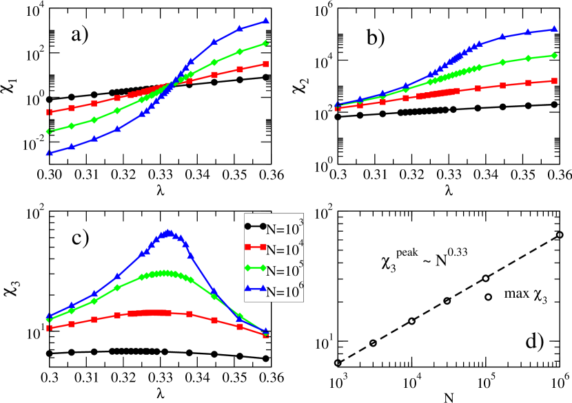
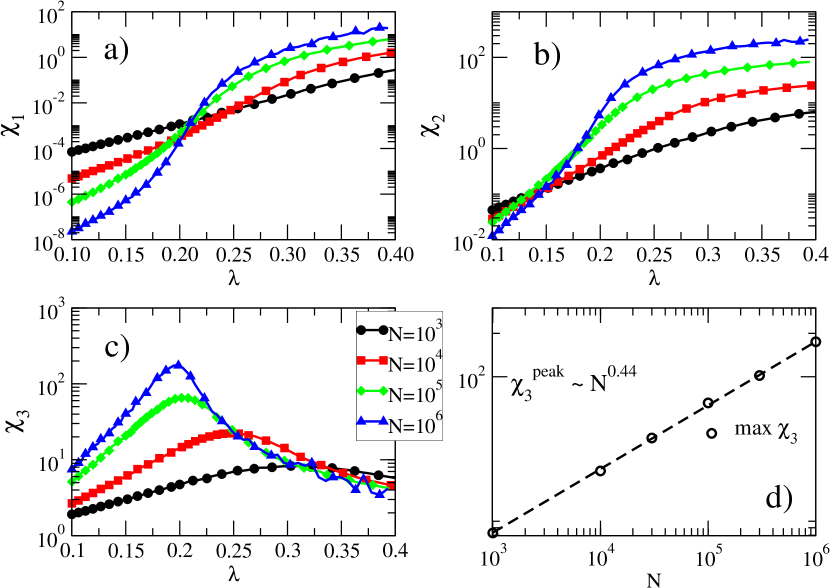
In Figs. 8 and 9 we plot the three susceptibilities as a function of the spreading rate $\lambda$ in different network sizes, for the RRN and UCM cases, respectively. Figures shows that $\chi_{3}$ exhibits a well pronounced maximum, $\lambda_{c}(N)$, growing with $N$; $\chi_{2}$ instead does not possess a maximum. In the case of RRN, where $\beta=\gamma$, $\chi_{1}$ does not exhibit a maximum either, but the critical point can be detected as the point where curves for different values of $N$ meet. This is not possible in UCM networks, where $\beta>\gamma$.

Assuming a FSS hypothesis for $\chi_{3}$ of the form

$$N^{-\beta/\nu}\chi_{3}(\lambda,N)=F[(\lambda-\lambda_{c})N^{1/\nu}],$$ (52)

implies that the height of the susceptibility peak $\chi_{3}^{\mathrm{peak}}=\chi_{3}(\lambda_{c}(N))$, scales as

$$\chi_{3}^{\mathrm{peak}}\sim N^{\beta/\nu}.$$ (53)

From here, using a linear regression in logarithmic scale, we obtain the estimates $\beta/\nu=0.33(1)$ for the RRN, and $\beta/\nu=0.44(2)$ for UCM networks, in reasonable agreement with the theoretical values $\beta_{\mathrm{th}}/\nu_{\mathrm{th}}=1/3$ and $\beta_{\mathrm{th}}/\nu_{\mathrm{th}}=0.40$, respectively, see Figs. 8(c) and 9(c).

As in the case of percolation we can fit the position $\lambda_{c}(N)$ of the peak of the susceptibility $\chi_{3}$ to formula analogous to Eq. (36) to obtain the values of the asymptotic critical point $\lambda_{c}$ and of the exponent $\nu$.

Figure 10: Plot of the peak position as a function of $N$ for the SIR dynamics on RRN (a) and UCM networks with degree exponent $\gamma_{d}=3.5$ (b). The linear behaviors are in agreement with Eq. (36).

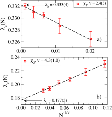
From such a non-linear fitting, see Fig. 10, we obtain for RRN the value $\nu=2.4(5)$ and a critical point $\lambda_{c}=0.333(4)$. For UCM we obtain instead $\nu=4.3(1.0)$ and $\lambda_{c}=0.177(5)$. In both cases there is a fair agreement with the expected theoretical values.

Figure 11: Data collapse analysis of the susceptibility $\chi_{3}$ for SIR model on RRN networks with degree $K=5$. We have used the exact theoretical values $\lambda_{c}^{\mathrm{RRN,th}}=1/3$, $\nu_{\mathrm{th}}=3$, $\beta_{\mathrm{th}}/\nu_{\mathrm{th}}=1/3$.

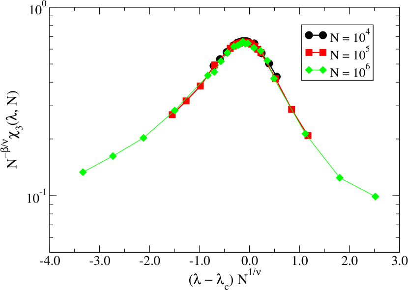
Performing a data collapse analysis, according to Eq. (52), we observe that data for RRN exhibits, as in the case of percolation, an almost perfect collapse using the exact theoretical values $\lambda_{c}^{\mathrm{RRN,th}}=1/3$, $\nu_{\mathrm{th}}=3$, and $\beta_{\mathrm{th}}/\nu_{\mathrm{th}}=1/3$, see Fig. 11.

Figure 12: Data collapse analysis of the susceptibility $\chi_{3}$ for SIR model on UCM networks of degree exponent $\gamma=3.5$. We have used the numerical epidemic threshold $\lambda_{c}^{\mathrm{UCM}}=0.185(5)$ and the exponents $\nu=4.3(5)$, $\beta/\nu=0.43(3)$.

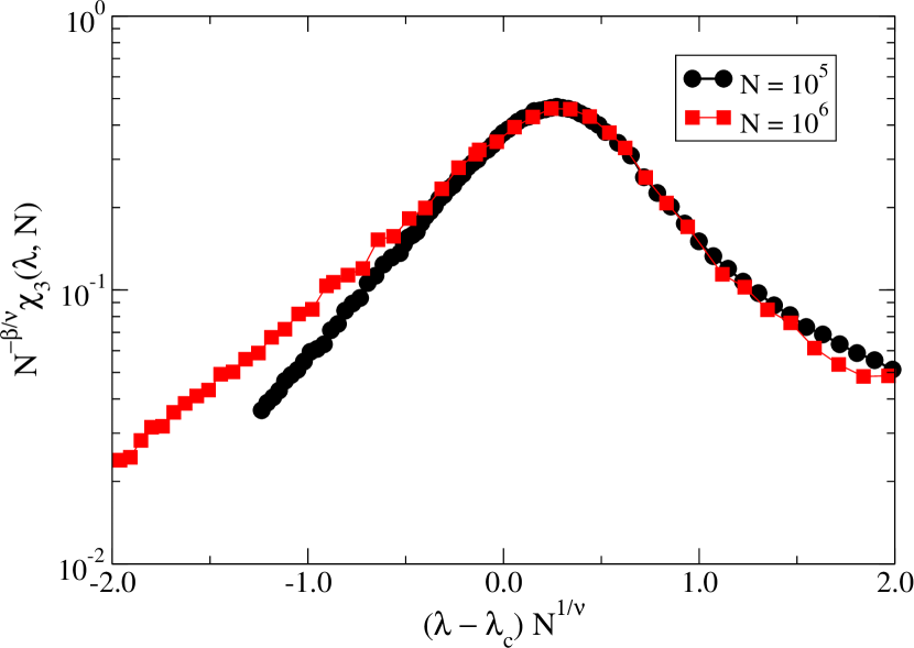
In the case of scale-free UCM networks, neither the theoretical predictions nor the numerically estimated parameters provide a good collapse of the susceptibilities $\chi_{3}$ for different network sizes. This is again due to the uncertainties in the position of the epidemic threshold, which are perceptible in the single network sample data used of the collapse. In this case, we proceed to estimate the best collapse by minimizing the distance between the rescaled plots using the Nelder-Mead unconstrained optimization algorithm, as implemented in the Python package fssa. The best collapse is obtained using the values $\lambda_{c}^{\mathrm{UCM}}=0.185(5)$, $\nu=4.3(5)$ and $\beta/\nu=0.43(3)$. The exponents are quite close to the theoretical predictions. With respect to the value of the numerical epidemic threshold, we can compare it with the numerical critical point obtained for percolation by noticing that, from Eqs. (17) and (9), we have

$$\frac{1}{\lambda_{c}}=\frac{1}{p_{c}}-1.$$ (54)

Using the numerical percolation value for UCM networks, $p_{c}^{\mathrm{UCM}}\simeq 0.153$ in Eq. (54), we obtain $\lambda_{c}^{\mathrm{UCM}}\simeq 0.181$, in good agreement with the best critical point from the data collapse analysis.

Finally, in analogy with the case of percolation we consider also an additional quantity, analogue to Binder’s cumulant. In view of the scalings in Eq. (42), the quantity

$$\chi_{4}=\frac{\left\langle{\overline{\phi}}\right\rangle^{3}}{\left\langle{\overline{\phi^{2}}}\right\rangle^{2}}$$ (55)

should scale at criticality as $N^{1-(2\beta/\nu+\gamma/\nu)}$ and hence be constant due to the hyperscaling relation Eq. (31). In Fig. 13 we plot the behavior of this analogue of Binder’s cumulant for this dynamics in the vicinity of the critical point. For RRN this quantity allows to determine with excellent precision the location of the critical point as the intersection of the curves for different size $N$. In the case of UCM instead, the presence of large sample-to-sample fluctuations spoils the determination of a single intersection point. In this case, even averaging the value of $\chi_{4}$ over several realizations does not lead to a reliable estimate of the critical point.

Figure 13: Close up of the quantity $\chi_{4}$ in the vicinity of the critical point for RRN networks (a) and UCM networks with $\gamma_{d}=3.5$ (b). In this last case, we consider the average over at least $10$ different network samples.

4 Discussion and conclusions

The numerical evaluation of epidemic thresholds in networks represents an important issue, with practical implications in real world situations Pastor-Satorras:2014aa . Despite this fact, in the case of the SIR model no clear prescription has been defined so far, and several alternative approaches Marrobook ; Ferreira12 ; Colomer-de-Simon2014 ; PhysRevE.91.010801 ; Crapey2006 ; Shu15 have been proposed and applied in the literature, based on the use of a ”susceptibility” measure, defined as a quantity that, as a function of the spreading rate (in the SIR model) or the occupation probability (for percolation), ought to show a maximum located in the vicinity of the putative critical point, while decreasing to a constant value away from it, in a similar fashion as the susceptibility usually considered in equilibrium statistical mechanics yeomans . In the present paper we have performed a theoretical analysis of different forms of susceptibilities that have been applied to study the SIR model and the related percolation process. The analysis of three possible candidate susceptibilities indicates that different forms of susceptibility are better suited to analyze percolation or the SIR process. More specifically, the susceptibility $\chi_{3}$, Eq. (26), is the correct one for the SIR model, while the susceptibilities $\chi_{1}$, Eq. (23), and $\chi_{2}$, Eq. (24) are better suited for percolation, the latter outperforming the former due to its fastest divergence at criticality. This different performance is traced back to the different nature of the numerical observables in SIR and percolation. While both models can be exactly mapped one onto the other, different observables can be measured for each of them in numerical simulations. So, while for the percolation process one can easily extract the largest cluster of each percolation sample in order to define an order parameter, and perform averages restricted over it, in the SIR process such distinction is impossible, and one is forced to define an order parameter in terms of averages over all outbreaks (clusters), sampled intrinsically with a probability proportional to their size.

Figure 14: Order parameter $\left\langle{\overline{\phi}}\right\rangle$ (average outbreak size) for the SIR model on RRN with degree $K=10$ as a function of $\lambda-\lambda_{c}$. The dashed line represent the behavior $(\lambda-\lambda_{c})^{2}$.

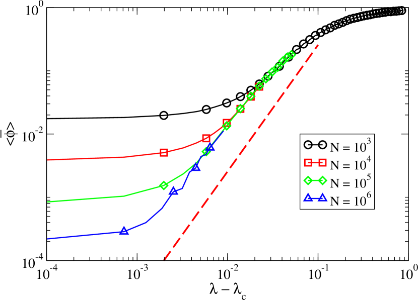
An additional consequence of the biased sampling of clusters in the SIR model is an effect regarding the determination of the exponent $\beta$, associated to the growth of the order parameter in the supercritical phase. When using the natural definition of the order parameter for the SIR model, given by the average relative outbreak size, $\left\langle{\overline{\phi}}\right\rangle$, from Eq. (38) we get, in the supercritical phase

$$\left\langle{\overline{\phi}}\right\rangle=\frac{\left\langle{G^{2}}\right\rangle}{N^{2}}\sim\left[\lambda-\lambda_{c}\right]^{2\beta}.$$ (56)

As a consequence, if the order parameter $\left\langle{\overline{\phi}}\right\rangle$ is plotted versus $\lambda-\lambda_{c}$ an effective exponent $\beta_{SIR}=2\beta$ is found. This is confirmed in Fig. 14, where we present results from simulations of the SIR process on RRN with fixed degree $K=10$, for which $\beta=1$. This result by no means invalidates the connection between SIR and percolation. It is only a consequence of the unavoidable bias in the selection of percolation clusters induced by the random choice of the initial seed of SIR outbreaks. On the other hand, Fig. 14 could potentially cast some doubts on the validity of the HMF prediction for the exponent $\beta$ refId0 , which coincides with the prediction in Eq. (10). A closer scrutiny shows however that the HMF prediction for SIR is correct: The order parameter considered in the HMF theory is not $\left\langle{\overline{\phi}}\right\rangle$, the average outbreak size, but rather the probability that, at the end of the outbreak, a randomly chosen node is recovered. In the thermodynamic limit $N\to\infty$, above the critical point, this quantity coincides with the relative size of the giant component of the corresponding percolation problem. This explains why the critical exponent $\beta$ found by HMF theory for SIR rightly coincides with the $\beta$ of bond percolation and is equal to a half of the exponent found in SIR numerical simulations for the order parameter $\left\langle{\overline{\phi}}\right\rangle$ determined numerically.

The analysis presented here allows finally to reinterpret and clarify some results appeared in the literature. In Ref. Shu15 it was found numerically that epidemic variability $\chi^{\prime}_{3}$ Crapey2006 provides precise estimates of the SIR epidemic threshold, while using $\chi_{2}$ leads to systematic errors. The scaling analysis performed in Sec. 3.2 allows to understand the reasons of this observation. On the other hand Ref. Lagorio2009755 observed that the average outbreak size does not correspond to the order parameter in percolation, in agreement with the discussion above. The authors of Lagorio2009755 provide a numerical technique to make these two quantities coincide: fix an outbreak size threshold $s_{c}$, and perform averages only over outbreaks larger than this threshold. Again, our results justify this recipe: The threshold introduced biases the clusters averaged towards the theoretical largest cluster, which is indeed the observable used to determine the order parameter in percolation.

Author Contribution Statement

All authors contributed equally to the paper.

References

- (1) M. Jackson, Social and Economic Networks (Princeton University Press, Princeton, 2010)
- (2) R. Pastor-Satorras, C. Castellano, P. Van Mieghem, A. Vespignani, Rev. Mod. Phys. 87, 925 (2015)
- (3) R. Pastor-Satorras, A. Vespignani, Phys. Rev. Lett. 86, 3200 (2001)
- (4) C. Castellano, R. Pastor-Satorras, Phys. Rev. Lett. 105, 218701 (2010)
- (5) O. Diekmann, H. Heesterbeek, T. Britton, Mathematical Tools for Understanding Infectious Disease Dynamics (Princeton University Press, Princeton, USA, 2012)
- (6) Y. Moreno, R. Pastor-Satorras, A. Vespignani, Eur. Phys. J. B 26, 521 (2002)
- (7) A.L. Lloyd, R.M. May, Science 292, 1316 (2001)
- (8) M. Boguñá, R. Pastor-Satorras, A. Vespignani, Epidemic spreading in complex networks with degree correlations, in Statistical Mechanics of Complex Networks, edited by R. Pastor-Satorras, J.M. Rubí, A. Díaz-Guilera (Springer Verlag, Berlin, 2003), Vol. 625 of Lecture Notes in Physics, pp. 127–147
- (9) S.N. Dorogovtsev, A.V. Goltsev, J.F.F. Mendes, Rev. Mod. Phys. 80, 1275 (2008)
- (10) M. Boguñá, C. Castellano, R. Pastor-Satorras, Phys. Rev. E 79, 036110 (2009)
- (11) M.E.J. Newman, Phys. Rev. E 66, 016128 (2002)
- (12) S.N. Dorogovtsev, J.F.F. Mendes, Advances in Physics 51, 1079 (2002)
- (13) C. Lagorio, M. Migueles, L. Braunstein, E. López, P. Macri, Physica A 388, 755 (2009)
- (14) P. Colomer-de Simon, M. Boguñá, Phys. Rev. X 4, 041020 (2014)
- (15) F. Radicchi, Phys. Rev. E 91, 010801 (2015)
- (16) P. Shu, W. Wang, M. Tang, Y. Do, Chaos 25, 063104 (2015)
- (17) J.L. Cardy, ed., Finite Size Scaling, Vol. 2 of Current Physics-Sources and Comments (North Holland, Amsterdam, 1988)
- (18) D. Stauffer, A. Aharony, Introduction to Percolation Theory, 2nd edn. (Taylor & Francis, London, 1994)
- (19) M. Newman, Networks: An Introduction (Oxford University Press, Inc., New York, NY, USA, 2010)
- (20) D.S. Callaway, M.E. Newman, S.H. Strogatz, D.J. Watts, Phys. Rev. Lett. 85, 5468 (2000)
- (21) R. Cohen, D. ben-Avraham, S. Havlin, Phys. Rev. E 66, 036113 (2002)
- (22) F. Radicchi, C. Castellano, Nat. Commun. 6, 10196 (2015)
- (23) Z. Wu, C. Lagorio, L.A. Braunstein, R. Cohen, S. Havlin, H.E. Stanley, Phys. Rev. E 75, 066110 (2007)
- (24) M. Boguñá, R. Pastor-Satorras, A. Vespignani, Eur. Phys. J. B 38, 205 (2004)
- (25) D. Ludwig, Math. Biosci. 23, 33 (1975)
- (26) P. Grassberger, Math. Biosci. 63, 157 (1983)
- (27) D.R. Cox, Renewal Theory (Methuen, London, 1967)
- (28) E. Kenah, J.M. Robins, Phys. Rev. E 76, 036113 (2007)
- (29) J. Marro, R. Dickman, Nonequilibrium phase transitions in lattice models (Cambridge University Press, Cambridge, 1999)
- (30) S.C. Ferreira, C. Castellano, R. Pastor-Satorras, Phys. Rev. E 86, 041125 (2012)
- (31) P. Crépey, F.P. Alvarez, M. Barthélemy, Phys. Rev. E 73, 046131 (2006)
- (32) A. Coniglio, D. Stauffer, Lett. Nuovo Cimento 28, 33 (1980)
- (33) R. Botet, J. Phys.: Conf. Ser. 297, 012005 (2011)
- (34) K. Binder, Z. Phys. B Con. Mat. 43, 119 (1981)
- (35) D.P. Landau, K. Binder, A guide to Monte Carlo simulations in statistical physics (Cambridge University Press, Cambridge, 2014)
- (36) R. Dickman, J. Kamphorst Leal da Silva, Phys. Rev. E 58, 4266 (1998)
- (37) M.E. Newman, R.M. Ziff, Phys. Rev. Lett. 85, 4104 (2000)
- (38) M. Newman, R. Ziff, Phys. Rev. E 64, 016706 (2001)
- (39) M. Catanzaro, M. Boguñá, R. Pastor-Satorras, Phys. Rev. E 71, 027103 (2005)
- (40) J.M. Yeomans, Statistical mechanics of phase transitions (Oxford University Press, Oxford, 1992)