Explosive transitions in complex networks’ structure and dynamics: percolation and synchronization
Abstract
Percolation and synchronization are two phase transitions that have been extensively studied since already long ago. A classic result is that, in the vast majority of cases, these transitions are of the second-order type, i.e. continuous and reversible. Recently, however, explosive phenomena have been reported in complex networks’ structure and dynamics, which rather remind first-order (discontinuous and irreversible) transitions. Explosive percolation, which was discovered in 2009, corresponds to an abrupt change in the network’s structure, and explosive synchronization (which is concerned, instead, with the abrupt emergence of a collective state in the networks’ dynamics) was studied as early as the first models of globally coupled phase oscillators were taken into consideration. The two phenomena have stimulated investigations and debates, attracting attention in many relevant fields. So far, various substantial contributions and progresses (including experimental verifications) have been made, which have provided insights on what structural and dynamical properties are needed for inducing such abrupt transformations, as well as have greatly enhanced our understanding of phase transitions in networked systems. Our intention is to offer here a monographic review on the main-stream literature, with the twofold aim of summarizing the existing results and pointing out possible directions for future research.
1 Introduction
1.1 Phase transitions
With the term phase of a system physicists actually denote one of its states, characterized by a set of physical properties that can be there considered as uniform over a macroscopic length scale.
Now, from the melting of ice into water to ferro-magnetism and from superconductivity to protein folding, nature is daily exhibiting phase transitions, i.e. processes in which systems drastically change one or many of their physical properties when a minimal variation in one of their control variables occurs.
In simpler cases, such transitions are described by the variation of the so called order parameter (a scalar, or a vector, or even a tensor measuring the degree of order in the system, whose magnitude normally ranges between zero in one phase and nonzero in the other), as the control variable (or the control parameter) is gradually and adiabatically changed.
More precisely, let us exemplify the simplest case of a system having only two phases (say phase 1 and phase 2), and passing from one to another with a process involving scalar control and order parameters. To gather a quantitative description and characterization of the transition, the following procedure is usually run after: i) the system is prepared in one of its two phases (say phase 1), which actually corresponds to set a specific initial value of the control parameter; ii) the control parameter is then gradually changed (increased, or decreased, depending on the particular case) in very small steps, up to the point at which the other phase is attained; iii) the corresponding variations of the order parameter are monitored. This procedure can be followed by starting either from phase 1 or from phase 2, producing the curves that describe the forward and backward transitions, respectively.
Now, a fundamental concept in statistical mechanics is that of reversibility of a given process, which, indeed, can be carried out reversibly or irreversibly. Reversibility can be attributed to processes which, after having taken place from an initial system’s phase, can be fully reversed, i.e. they can be brought back to their original phase via the exactly opposite transition, and with no changes in either the systems or their surroundings. In our case (as well as it happens in many other circumstances) reversibility consists in a full equivalence of the two curves obtained during the forward and backward transitions. When, instead, transitions are irreversible, the two forward and backward curves differ, and a wealth of interesting and relevant events, such as hysteretic loops, occur.
Given the ubiquitous presence of phase transitions in the real world, it is not strange that physicists started, since the very beginning of statistical mechanics, to delve into discovering universal and critical behaviors (or scaling properties in the proximity of the transition points), as well as to pay effort in classifying phase transitions. The first attempt of providing a classification was given by Ehrenfest [1], but more modern classification schemes consider phase transitions as divided into two broad categories: the first-order and the second-order ones.
In thermodynamics, first-order phase transitions are those that involve a latent heat, i.e. those during which the system either absorbs or releases a typically large amount of energy per volume. Normally, they are characterized (at the transition point) by a “mixed-phase regime”, in which some parts of the system have completed the transition and others have not, this way featuring a sort of coexistence of the two system’s phases. Signatures of such transitions are the abrupt and discontinuous behavior of the order parameter in the proximity of the transition point, as well as the intrinsic irreversibility of the transition, with the presence (in the majority of the cases) of hysteretic loops. At variance, second-order phase transitions (also called continuous phase transitions) are reversible, and correspond to order parameters displaying a continuous behavior near criticality. Examples of the former processes are the melting of ice, or the boiling of water, or the super-cooling and super-heating transitions. Examples of the latter processes are the ferromagnetic transition, the super-conducting transition, and the super-fluid transition.
1.2 Percolation and synchronization
Our main scope is reviewing recent progresses on two classical phase transitions taking place in networked units (percolation and synchronization), as well as on how they can in fact be rendered explosive, i.e. first-order-like.
Percolation (from the Latin percolare, which means “to filter” or “to trickle through”) is a transition involving a drastic change in the network’s structure, due to the emergence of a giant connected component whose size is of the order of the network’s size. By means of percolation, a phase of the network where fragmented portions, or clusters, are isolated is changed into a fully connected structure, where nodes can globally interact. The process can be conducted in two ways: either starting from isolated nodes and adding gradually links (what is called bond percolation), or sequentially adding nodes to the graph (what is called site percolation).
Synchronization (from the Greek ς\acctonosυγ=together and χρόνος=time) is instead a process having to do with network’s dynamics. There, dynamical systems adjust some properties of their trajectories (due to their interactions, or to a driving force) so that the network eventually operates in a collective and macroscopically coherent way.
Percolation and synchronization are nowadays classical fields of study in statistical mechanics, and an interested reader can find orientation within the wealth of currently available results in various monographic papers and books [2, 3, 4, 5, 6, 7, 8].
A common result is that the vast majority of transitions to percolation and synchronization are of the second-order type, continuous and reversible. However, as soon as networked units with complex architectures of interaction are taken into consideration, two abrupt and explosive phenomena have been recently reported, namely explosive percolation [9, 10, 11, 12, 13] and explosive synchronization [14, 15, 16, 17, 18, 19, 20, 21, 22], which rather remind first-order like transitions. Explosive percolation (a sudden materialization of a giant connected component in the structure of the network) was discovered in 2009 [9], while explosive synchronization (an abrupt emergence of a collective, synchronized, behavior in network’s dynamics) was first described already in 1984 [23]. In literature, the use of the jargon first-order like purports that those explosive processes fulfill some of the properties of a first order transition in thermodynamics (as, for instance, discontinuity and irreversibility) and yet they fail featuring all the attributes, qualities and traits of a true first-order transition.
Unveiling the main mechanisms at the origin of these two abrupt transitions is of fundamental relevance for a better understanding of networks’ structure and dynamics. For instance, explosive percolation is considered to be at the basis of phenomena such as cascading failures, which, on their turn, may have devastating effects (and cause huge economic losses) in various circumstances: electrical blackouts in power grids, financial crises in the network of global financial market, and the spreading of information and rumors through online social networks, such as Facebook or Twitter. On the other hand, synchronization is of primary importance in sustaining basic brain functions such as emotions, complex thoughts, memory, language comprehension, consciousness, etc., while clinical evidence seems to indicate that explosive synchronization is actually the mechanism underlying the transition from normal to pathological brain behavior during epilepsy, one of the world’s most prominent brain disorders.
Furthermore, when synchronization occurs through an irreversible transition, one interesting and ingenious application is the construction of magnetic-like states of synchronization in networked oscillators: setting the coupling strength inside the hysteresis region of the transition, and entraining (through a unidirectional coupling with an external pacemaker) the phases of the oscillators, the system can be forced to pass from the unsynchronized to the phase-locked configuration, which (once the pacemaker is later switched off) remains actually unalterable (like the case of a permanent magnet).
Given, therefore, their relevance to practical applications, explosive percolation and synchronization have attracted a comprehensive and lasting attention in various fields, and have stimulated a large amount of exciting works and debates. The result is that many substantial contributions and progresses (including experimental verifications) are today available, which provide a rather deep insight on the crucial structural and dynamical mechanisms at the basis of the abruptness of the two transitions.
It is therefore now the time to offer a comprehensive review on the current state of the art on the subject, which would offer a reflected and thought out viewpoint on the many achievements and developments (summarizing the existing models and results), as well as a weighted and meditated outlook to the still open questions and to the possible directions for future research.
1.3 Outline of the report
After the present introduction, the review is organized as follows. In Chapter 2, the main results on explosive percolation are summarized and discussed. Starting from the seminal work by Achlioptas, the Chapter gives a survey on the various processes that have been proposed in order to produce abruptness in the percolation transition, as well as it critically examines the essential physical mechanisms which are at the origin of the explosiveness. The Chapter ends with accounting for the debate stirred within the scientific community, and reports some rigorous conclusions that have been ultimately made on the nature of the transition in the thermodynamic limit (i.e. for systems whose size tends to infinity).
Chapter 3 contains a brief excursus on classical synchronization in both identical and non-identical networked systems. An interested reader can definitely find a much more detailed description of the subject in various other books and review articles, like those of Refs. [4, 5, 6, 7, 8], whereas Chapter 3 concentrates on the main ideas and concepts which are then conveniently recalled at the moment of describing those processes where synchronization emerges, instead, abruptly.
In Chapter 4, we provide a detailed overview of explosive synchronization. Starting from the early evidences of first order transitions in the thermodynamic limit of models of globally coupled phase oscillators (as well as from the seminal work of Ref. [14]), the Chapter describes the cases where the transition to synchronization is first-order-like, and discusses the generality of explosive synchronization in networked systems with complex architectures and topologies. The Chapter, furthermore, gives an account of some recently discovered and unveiled coherent states (the Bellerophon states), whose existence is intimately related to the possibility for the system to feature explosive transition to synchronization.
Chapter 5 is an exhaustive journey on the applications of explosive percolation and synchronization. In particular, applications of explosive percolation are presented in cascading failures of inter-connected multi-layer networks (of relevance in technology and biology), and applications of explosive synchronization are described in power and smart grids, and in brain dynamics. The Chapter accounts also for experimental realizations of explosive synchronization in controlled laboratory systems.
Finally, Chapter 6 presents our conclusive remarks and perspective ideas on yet open problems to solve, and on possible research lines for the future of the subject.
For the reference of the reader, we summarize here below (in Table 1) the list of major symbols and abbreviations which are used all throughout the Manuscript.
| Nomenclature | Abbreviations | ||
| Adjacency matrix | 2D | Two dimensional | |
| Node degree | 3D | Three dimensional | |
| Network average degree | AP | Achlioptas process | |
| Degree distribution | BA | Barabási-Albert | |
| Degree-degree correlation | BF | Bohman-Frieze | |
| Eigenvalues of the adjacency matrix | BFW | Bohman-Frieze-Wormald | |
| Number of edges | CA | Coauthorship | |
| Coupling strength, synchronization control parameter | CM | Configuration Model | |
| System size | CS | Complete Synchronization | |
| Oscillator phase | CPT | Continuous Phase Transition | |
| Oscillator phase in the rotating frame | DPT | Discontinuous Phase Transition | |
| Frequency | dCDGM | da Costa-Dorogovtsev-Goltsev-Mendes | |
| Natural frequency | DLCA | Diffusion-limited cluster aggregation | |
| Natural frequency distribution | EP | Explosive Percolation | |
| Average phase | ER | Erdös-Rényi | |
| Average frequency | ES | Explosive Synchronization | |
| Kuramoto Order Parameter | GAP | Generalized Achlioptas process | |
| Percolation order parameter | H-PHN | Human protein homology network | |
| Size of the largest cluster | LCC | Largest Connected Component | |
| Size of a network cluster | MC | Minimum Cluster | |
| Time, percolation control parameter () | MSF | Master Stability Function | |
| PR | Product Rule | ||
| PT | Phase Transition | ||
| SCA | Spanning Cluster-Avoiding | ||
| SF | Scale-Free | ||
| SP | Suppression Principle | ||
| SR | Sum Rule | ||
| SW | Small-world | ||
| TR | Triangle Rule | ||
| TW | Traveling Wave | ||
2 Explosive percolation
2.1 Introduction and historical overview
Percolation transition refers to the emergence of a giant connected cluster (or giant connected component) in a lattice, or a network, when bonds/sites are gradually occupied at random. For simplicity (and unless mentioned otherwise), throughout this review we always consider bond percolation (i.e. the process through which the nodes of a network are fixed, and links, or bonds, are gradually added).
In bond percolation, one then starts from unconnected nodes. At each time step, an edge is added between two nodes selected according to a given rule. The number of edges () added to the system at a certain time step divided by the system size () is the control parameter () that describes the phase transition (PT). As for the order parameter (usually denoted as ) one can take the fraction of nodes belonging to the giant cluster (the largest cluster) in the network. As time increases, more and more edges are formed in the network, which causes the order parameter to increase from zero. In the thermodynamic limit (), exhibits a PT from zero to at a critical point .
Classical percolation is a typical geometrical PT, which has been extensively studied since 1940’s in many fields, including mathematics, statistical physics, and engineering. Numerous percolation models, such as invasion percolation, first-passage percolation, directed percolation, bootstrap percolation, -core percolation have been developed, and it has been shown that PT is closely related to various applications, such as conducting materials, fractality of coastlines, turbulence, magnetic models, colloids, growth models, watersheds of landscapes, the spin quantum Hall transition, etc. The reader is addressed to recent reviews in Refs. [24, 25, 26, 27] and references therein for an overview of the main results and concepts about classical percolation.
In modern statistical physics, PTs are traditionally classified into two types, namely, the continuous PT (CPT) and the discontinuous PT (DPT), which are also known as the second-order PT and the first-order PT, respectively. CPT exhibits universal characteristics, and can thus be categorized into different universality classes. At variance, DPT is non-universal. There are many ingredients that determine whether a phase transition occurs in a system via a CPT or DPT, such as, for instance, dimensionality, the type of the dynamical rules, as well as the underlying network’s structures.
For decades, most transitions in classical (or ordinary) percolation have been shown to be of CPT (the second-order) type. One example is the prototypical bond percolation in Erdös-Rényi (ER) networks, for which the size of the giant cluster smoothly increases as the control parameter exceeds the percolation threshold. For , the order parameter increases with as . It should be pointed out, however, that there are also rare examples of percolation models that exhibit DPT, such as the bootstrap percolation [28, 29], the -core percolation [30, 28, 31], and the jamming percolation [32].
In 2009, a competitive percolation process was introduced, later known as the Achlioptas process (AP) [9]. AP is essentially different from traditional uncorrelated percolation models. Indeed, at each time step, two edges are first randomly selected as potential candidates. Then, a product rule (PR) is applied: the candidate edge that actually minimizes the product of the sizes of the two clusters containing its end points is eventually established, while the other one is disregarded. An alternative is the sum rule (SR) in which the established link is the one that minimizes the sum of the two clusters’ sizes. In AP, a giant cluster emerges after a number of steps that is much smaller than the system size. As a consequence, the order parameter exhibits an extremely abrupt “jump” at the percolation point. At first glance, such a behavior resembles a discontinuous transition and this is the reason why AP was termed “explosive percolation” (EP) [9]. As we will see later on (in Section 2.7), EP can actually be a CPT, or a genuine DPT.
After the initial work by Achlioptas [9], extensive studies on EP have been carried out in various configurations, such as 2D lattices [33, 34, 35, 36, 12, 37, 38, 39, 40, 41, 42], 3D or high-D lattices [42], Bethe lattices [43], ER networks [9, 34, 44, 45, 13, 12, 46, 47, 39], scale-free (SF) networks [48, 49, 34], and real-world networks [50, 51].
The key factor in AP is the competition (at each time step) between two potential edges before the actual selection of the one which is added to the network. Such a competition mechanism can be straightforwardly extended from two to more edges, leading to the so called “best-of-” rule, where potential edges are first chosen at each time step. Then, the candidates are evaluated using either PR or SR, and the one minimizing the product or the sum of the two end clusters is eventually established. For this reason, the algorithm is also known as the “min-cluster-” rule. In the limit case where , the “min-cluster-” rule becomes the smallest cluster model [52], i.e., at each time step the two smallest clusters in the network are identified to connect. So far, the “best-of-” rule has been studied in 2D lattices [53, 54, 55], 3D lattices [55], ER networks [52, 13, 46, 56, 57], and real-world networks [58, 51].
Other generalized Achlioptas processes (GAP) have been proposed and investigated, including the da Costa-Dorogovtsev-Goltsev-Mendes (dCDGM) model [11] and the -vertex model [59, 60, 61], which has (for ) several variants, such as the adjacent edge rule [62], the triangle rule (TR) [62, 59], and the clique-3 competition rule [46]. All GAP models have been studied in 2D lattices [41], in ER networks [11, 62, 46, 13, 47, 39, 59, 60, 61, 63, 64, 65, 66, 67], and in real-world networks [68].
The relevant literature regarding AP and GAP models is summarized in Table 2, where the reader can visually (and easily) find information on which specific model has been adopted in which specific network’s topology.
| Model | Lattice () | Lattice () | Other Lattices | Random | SF | Others |
|---|---|---|---|---|---|---|
| Product rule | [33, 34, 35, 12, 37, 38, 39, 40, 41, 42] | [42] | [43] | [9, 34, 44, 45, 13, 12, 46, 47, 39] | [48, 49, 34] | [50, 51] |
| Sum rule | [36, 40, 42] | [42] | [43] | [9, 13, 12, 47] | ||
| Best-of- | [53, 54, 55] | [55] | [52, 13, 46, 56, 57] | [58, 51] | ||
| dCDGM | [11, 47, 39, 64, 65, 66, 67] | [68] | ||||
| -vertex | [62, 46, 13, 59, 60, 61, 69] |
The fundamental difference between classical percolation and AP is that the latter follows a competitive (or correlated) rule, which involves non-local (or even global) information on the graph. It is well known that introducing long-range interactions during percolation can change the universality class of the PT, or even the transition type. Thus, it is not surprising that a percolation model with non-local competition (like AP) can give rise to abrupt transitions. Following the same motivation, many other models were also investigated, in which various constraints on the occupation of edges were proposed. These models include the Bohman-Frieze-Wormald (BFW) model [13, 70, 71, 72, 73, 69, 74, 75, 76], the probability model [77, 78, 79, 80, 53, 81, 56, 82]), the hybrid model [53, 83, 84, 25], the diffusion-limited cluster aggregation (DLCA) model [10, 85], the spanning cluster-avoiding (SCA) model [86, 87], the two-species cluster aggregation model [88], the bootstrap model [89], the -core model [83, 90, 91, 92], the cascading failure model in inter-dependent networks [93, 94, 95, 96, 97, 98, 99, 100, 101], and others [102, 103, 104, 105]. The relevant literature regarding all these other models is summarized in Table 3. Like in the case of Table 2, the reader can find orientation on the various adopted models and network structures.
Let us now briefly discuss the mechanisms leading to EP. In classical percolation, nodes are progressively chosen at random to connect. Thus, the probability to establish a specific edge is proportional to the product of the sizes of the clusters where the edge’s end points reside. The result is that a giant cluster can quickly form, and this in turn amplifies the probability for its further expansion. It is therefore expected that CPT always occurs under this scheme.
In AP and GAP models, instead, competition among potential edges is introduced at the basis of the cluster-merging processes. The key factor leading to EP is here that the competition mechanism systematically suppresses the formation of large components [78, 77, 47, 86], and such a suppression principle generates the necessary “powder keg” (i.e., abundant small-sized clusters) in a specific range before the onset of the transition [52]. Typically, after a number of steps, such small/medium sized clusters merge to each other, and a giant cluster suddenly emerges. Similar suppressive mechanisms have also been pointed out to occur in the DLCA model [10], the spanning cluster-avoiding model [86], and the explosive synchronization model [19].
| Model | Lattice () | Lattice () | Other Lattices | Random | SW | SF | Inter-dependent |
|---|---|---|---|---|---|---|---|
| BFW | [71] | [71] | [71] | [13, 70, 75, 72, 73, 69, 74] | [76] | ||
| Probability | [77, 78, 80, 53] | [81] | [81] | [79, 77, 80, 56, 82] | |||
| Hybrid | [53, 83, 25] | [84, 83, 25] | |||||
| DLCA | [10, 85] | [85] | |||||
| SCA | [86, 87] | ||||||
| TCA | [88] | ||||||
| Bootstrap | [89] | ||||||
| -core | [83, 91] | [91] | [83, 91, 92] | [90] | |||
| Cascading failure | [106, 93, 94, 95, 96, 97, 98, 99, 100, 101] | ||||||
| Others | [102, 105] | [103, 104] |
In BFW models [73, 69], another underlying mechanism for EP (namely, the growth by overtaking) was revealed. In these models, the growth of the largest cluster is so severely limited by the edge selection rules that it can only merge with isolated nodes. As a consequence, all significant changes in the size of the giant cluster result from two smaller components merging together and overtaking the previous largest cluster to become the new largest component.
The central issue is whether or not EP is really a discontinuous transition, especially in the thermodynamic limit. Because of the extremely slow convergence to an asymptotic behavior (as the system size increases), it is difficult to determine the transition nature of EP with the only help of numerical simulations. Therefore, whether or not EP is a genuinely discontinuous transition became, for some time, the object of a controversial issue [11, 107, 12, 47, 13, 45, 37, 36]. Later, it was eventually revealed that the EP transition of Ref. [9] is in fact continuous in the thermodynamic limit [11].
The continuous character of EP was initially asserted on the basis of numerical results for a specific model [12], and later on it was further pointed out that EP under AP is continuous, but with a unusual finite size behavior. Namely EP under AP belongs to a new universality class with an extremely small exponent of the order parameter [11] . Numerical results give a power law with (close to ), for . It is therefore such a littleness of the exponent that leads to a large discrete jump in the order parameter, resembling a seeming discontinuity at the critical point.
Finally, based on numerical investigations regarding the average size of medium-sized cluster [52], Riordan and Warnke provided a mathematical proof that all AP models on ER networks give rise actually to continuous percolation transitions [13]. The proof reveals that the number of clusters participating in the merging process (needed to generate a macroscopic-sized cluster) is not sub-extensive to the system size, and therefore it cannot bring out a DPT in the thermodynamic limit. On the other hand, Ref. [13] also showed that, for a random network, if the number of competitive edges is allowed to increase with the system size in a way that as [for example, ], a true DPT can occur also in the thermodynamic limit.
It is today accepted that EP under Achlioptas processes are actually CPT (second-order), but with a universality class different from all the others previously observed [12]. The interested reader is addressed to Ref. [25] for a critical and exhaustive review on all critical exponents. While other GAP models (such as minimal cluster model [52] and dCDGM model [11]) turn out to generate explosive (but actually continuous) percolation transitions in finite size systems, it has been discovered that many alternative algorithms lead to genuinely DPT. These latter models include the BFW model [70], the Gaussian model [78], the spanning cluster-avoiding model [86], the hierarchical model [103], and the two-species cluster aggregation model [88].
The next Sections will expand the discussion on all the concepts, ideas and methods summarized so far.
2.2 Explosive percolation in the Achlioptas process
The percolation process introduced by Achlioptas can be described as follows [9]. The starting point is a network with vertices and no edges, and edges are added one by one. Precisely, at each time step, two potential edges and are arbitrarily chosen, each of which is supposed to connect two clusters (i.e. the two end points of each edge are supposed to belong to two distinct clusters). The size of a cluster is defined here as the number of nodes in it. Now, let us denote the sizes of the two end clusters linked by as and , and the sizes of the two end clusters linked by by and . In order to select the edge to be actually added to the network, , , , and are compared among them, by means of the use of certain rules. For instance, one can compare the products and . If (), then edge () is established and () is discarded. This rule is called “the product rule”, as one always establishes those links minimizing the product of the sizes of the two end clusters. If one instead replaces the “product” by the “sum” of the clusters’ sizes, the resulting rule is called the “sum rule”.

Figure 1 compares classical percolation and AP, and shows that the latter exhibits two distinguished characteristics. One is that the percolation threshold is significantly postponed (Fig. 1(c)). Another, and most important, is that the order parameter shows an extremely steep “jump” at the percolation point which, at first glance, seemingly resembles a DPT (Fig. 1(c)). In order to characterize the jump, Ref. [9] counts the fraction of vertices added in the network when the giant cluster grows from size at most to size at least . It is shown that at most steps are needed. This implies that, at the phase transition, a constant fraction of the vertices is accumulated into a single giant cluster within a sub-linear number of steps.
It should be emphasized that not all competitive rules lead to EP. Traditionally, the selecting rules in percolation models can be classified into two types. One is the “bounded-size rule”, in which decisions depend only on the sizes of the clusters, and all clusters with size greater than a certain constant are regarded as the same. For example, is the Bohman-Frieze (BF) rule, where is chosen if it joins two isolated vertices, otherwise is chosen. As shown in Fig. 1(c), the percolation under the BF rule turns out to be still continuous, but with a postponed threshold. In fact, it has been conjectured that the percolation transition is continuous for all bounded-size rules [108].
At variance, an “unbounded-size rule”, like the PR or SR in Ref. [9], treats all clusters of distinct sizes uniquely. Such unbounded-size rules typically lead to interesting transition behaviors, such as shifting the transition threshold and even yielding EP. Not all AP models lead to EP. For example, in the “largest-cluster rule” [9, 52], at each step one selects the two largest clusters in the network to connect. Apparently, the process seems to be similar to AP (due to the considered competitive rule for adding edges). However, the percolation turns out to be continuous under this rule.
PR and SR can be straightforwardly extended to the case where at each time step potential edges are chosen to compete. This leads to the “best-of- rule” or the “min-cluster- rule”, which typically leads to EP [52]. Note that when the “best-of- rule” recovers the ordinary random percolation, which is continuous. When , it specializes the PR/SR model studied in Ref. [9], which leads to EP. With increasing , the process becomes more and more competitive. If , where is the total number of nodes, we have global competition among all unoccupied links in the network. This limit situation corresponds to the “smallest-cluster rule” [52], where at each step two smallest clusters in the network are identified to be connected, and global information is used in order to identify the two smallest clusters [46].
2.3 Explosive percolation in generalized Achlioptas processes
Stimulated by the observation that non-local or global competition rules during cluster-merging processes can lead to EP, a number of generalized Achlioptas processes (GAP) have been studied. In the following, we briefly describe two generalizations of the original AP.
2.3.1 The dCDGM model
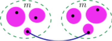
The model has been studied in Refs. [11, 47, 39, 68, 64, 65, 66, 67]. At each step, a pair of clusters are initially randomly selected, and the smaller cluster is kept. Then the same process repeats, and another (smaller) cluster is picked. In order to establish the link, one actually chooses two random nodes (one from each of the chosen clusters) and connects them. The above procedure is sequentially repeated. The dCDGM model provides even more stringent selection of small components during cluster-merging processes than usual AP, since it guarantees that the product of the sizes of the two merging clusters is the smallest of the four possibilities. This algorithm can be naturally extended to the case of nodes. For instance, Fig. 2 illustrates this process for [65].
2.3.2 The -vertex rule
In this second model, vertices are randomly chosen at each step, and two of them are connected with an edge using certain rules [60, 109, 59, 61]. Notice that the resulting percolation process includes the ER model, which is obtained for . Also, Achlioptas processes can be regarded as a special case of the 4-vertex rule. When , the rule has several variants, such as the triangle rule (TR) [62], the adjacent edge rule [62], and the clique-3 competition rule [46]. In all these variants, three distinct vertices are randomly selected at each step. Then, one examines the three possible edges (TR and clique-3 competition) or two adjacent edges in the triangle, and selects the edge that connects the two smallest components.
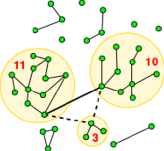
The bounded-size rule variant occurs when all components have size above the bound , and one chooses a random edge out of the three; if two components have size above the bound , one chooses a random edge out of the two adjacent of the smallest component. Furthermore, Nagler et al. have proposed a variant of the TR [59]. There, one first chooses three vertices at random and connects those two vertices that reside in clusters whose size difference is minimal (see Fig. 3). Notice that this latter model does not suppress the growth of the largest cluster, in contrast to many other Achlioptas processes. It is found that the continuous phase transition can have the shape of an incomplete devil’s staircase with discontinuous steps in arbitrary vicinity of the transition point [59].
2.4 Explosive percolation under other algorithms
Beyond ordinary percolation, many other models have been developed, where various constraints on the occupation of edges have been considered in order to produce EP. In the following, we briefly review some of these models.
2.4.1 The BFW model
In Ref. [70] a model is introduced (based on the work of Bohman, Frieze, and Wormald (BFW) [110]), where the members of a set of potential edges are considered one at a time, and either added to the network or rejected. Specifically, the algorithm of BFW is as follows. Initially, there are isolated nodes and all bonds are unoccupied (empty). Therefore, there are clusters of unitary size. At each time step, one edge is added to the network. Let be the total number of selected bonds, the number of occupied bonds, and the stage of the process, initially set to . The first bond is occupied at random, such that .
Then, at each step ,
-
1.
One edge is randomly selected out of all edges (or the unoccupied ones);
-
2.
The maximum cluster size is measured, if the selected edge is occupied;
-
3.
If , go to 4. Else, if , go to 5. Else, increment by one and go to (3);
-
4.
Occupy the selected edge;
-
5.
Increment by one.
The procedure is applied iteratively from (corresponding to a bond occupation fraction ) to (where all bonds in the system are occupied, i.e., ). Using such a model, Chen et al. have shown that multiple stable giant clusters can coexist, and the percolation transition is strongly discontinuous [70]. The BFW model has been extensively studied in various networks, including lattices and tree-like networks [71], ER networks [13, 70, 75, 72, 73, 69, 74], and SF networks [76]. Notice that in Refs. [110, 70, 73, 69, 74, 76] edges are randomly chosen from all edges (i.e. regardless on whether or not they are occupied), while in Refs. [71, 72] edges are only sampled from the set of unoccupied bonds. In Refs. [70, 71, 72, 76], . Later, generalizations of this function have been considered as [73], and [69, 74].
2.4.2 Probability models
In this type of models, an edge between a pair of clusters is occupied with certain probability at each time step. This process differs substantially from AP, since here all unoccupied connections can potentially be chosen at each step, though some of them with a much larger probability [77]. For instance, in cluster aggregation model [79, 80], all currently unoccupied edges are considered. Let one denote the sizes of the clusters to be connected by the edge as and . Each of these vacant edges is given a weight , and the sum over all the weights is calculated as a normalization constant . Then the edge is occupied with probability .
In the Hamiltonian model of Ref. [77], instead, one starts with a network of vertices without edges, so each vertex initially belongs to a different cluster. First, a simple Hamiltonian is defined as a function of the cluster sizes and of the number of redundant edges added to the clusters. Then, a new edge between any pair of vertices not yet connected is added, with a probability proportional to , where is the energy change after adding the edge.
Another model belonging to this class is the largest cluster model (or the Gaussian model) [78]. There, a link is randomly selected among the unoccupied ones. If its occupation would not lead to the formation or growth of the largest cluster, it is always occupied; otherwise, it is occupied with probability min. For , this probability suppresses the formation of a cluster significantly larger than the average, inducing a homogenization of cluster sizes, which is important to generate EP.
2.4.3 Hybrid models
Hybrid models are those for which the rule for the occupation of edges is a mixture of ordinary percolation and competitive rules: at each time step, an edge can be chosen randomly with probability , while it can also be chosen following a given competitive rule with probability . For example, in Refs. [84, 25], PR is used; in Ref. [53], the best-of-ten PR is used; in Ref. [83], a mixture of - and -core on the random network and a mixture of -core and jamming percolation models in 2D lattice are studied. Hybrid models have been studied in 2D lattices [53, 83, 25] and ER networks [84, 83, 25].
2.4.4 The diffusion-limited cluster aggregation (DLCA) model
In this model, studied in Refs. [10, 85, 27], single particles are initially randomly placed in a square lattice. The particles are assumed to be Brownian, so that the velocity of a cluster is inversely proportional to the square root of its size, i.e. the velocity of an -sized cluster is given in a general form as . As a consequence, the larger clusters move considerably more slowly. When two clusters become nearest neighbors, they merge and form a larger cluster. The Brownian motion suppresses the mobility of the largest clusters, impeding their growth, and leading to the discontinuous emergence of a giant cluster. Generalized Brownian motion, for which the velocity is inversely proportional to the size of the cluster to a power (i.e., ) gives rise to a tri-critical point that separates discontinuous from continuous transitions as a function of . Namely, as soon as is a tri-critical point, it is shown that when (), the PT is discontinuous (continuous) [10].
2.4.5 The spanning cluster-avoiding (SCA) model
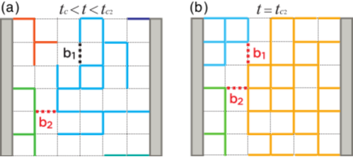
The SCA model, studied in Refs. [86, 87], considers percolation on an Euclidean lattice, where the emergence of a spanning cluster is concerned. In a spanning cluster, a path of activated links exists that connect sites from one side of the lattice to the other. Inspired by the best-of- rule, Cho et al. introduced a new global constraint for the dynamics. As shown in Fig. 4, at each time step , unoccupied edges are chosen randomly and classified into two types: bridge and non-bridge edges. Bridge (non-bridge) edges are actually those that would (would not) form a spanning cluster when occupied. The SCA model strictly avoids bridge edges to be occupied, and therefore one of the non-bridge edges is randomly selected and occupied. If the potential edges are all bridge edges, then one of them is randomly chosen and occupied. Once a spanning cluster is formed, no more restrictions are imposed on the occupation of edges. This procedure continues until all edges are occupied. Numerical simulations and theoretical results have shown that the EP in SCA model can be either discontinuous or continuous for , depending on the number of eligible edges . For , the transition is shown to be continuous for any finite and fixed value of . However if varies with the system size , a discontinuous transition can also take place for .
2.4.6 The two-species cluster aggregation model
In this model, studied in Ref. [88], initially isolated nodes are randomly separated into two populations: half of them is colored in black (B) and the other half in white (W), with all nodes in the same cluster keeping the same color. At each time step, the three possible combinations BB, BW, and WW are given selection probabilities , , and , respectively (where is a model parameter in the range ). Two clusters are then selected independently of the cluster sizes, and two nodes (one from each cluster) are selected randomly and connected, which causes the two clusters to merge. If the two selected clusters are the same, then two distinct nodes from that cluster are connected. Meanwhile, the colors of all the nodes in the resulting merged cluster have to be updated according to a certain rule. See Fig. 3 in Ref. [88] for an illustration of the algorithm. The cluster aggregation model can exhibit both type-I and -II DPT, as the model parameter changes [88].
2.4.7 The bootstrap models
In the context of EP, some bootstrap models have been proposed [89]. The standard bootstrap percolation process on a lattice assumes that sites are either active or inactive, and the state of a site depends on its neighbors. Initially, each site is activated with a probability , and inactivated with probability . Every activated site remains in its state, while each inactivated site can become active (and remain active forever) if its nearest neighbors are active (with ). The procedure is continued until the system reaches the stable configuration which does not change anymore. In the final state of the process, one is concerned on whether or not a spanning giant cluster of active sites exists. Bootstrap percolation can show either continuous or discontinuous transitions, depending on the type of networks (lattice or random), and on the dimensionality of the lattice.
2.4.8 The -core model
-core percolation [83, 90, 91, 92] is a model of correlated percolation beyond the ordinary one. The -core of a graph is the maximal subgraph for which all vertices have at least neighbors. It can be found as an asymptotic structure obtained by recursively removing all nodes whose neighbors are less than . For example, if , all leaves (nodes with only a connection) are removed in a first step. This might turn into some nodes (which originally had 2 or more neighbors) becoming leaves. Then, these latter nodes are removed in a second round, and if this again turns nodes into leaves, they are removed again, and so on. In this way, one ends up either with an empty cluster, or with a cluster where all nodes have neighbors, i.e., the 2-core. It has been proved that -core percolation on random networks exhibits a CPT for , and a DPT for [111]. However, unlike a typical DPT, not one but several diverging length scales exist such that the transition has an unusual nature [112].
2.4.9 Cascading failure model in inter-dependent networks
This type of models aims at studying processes such as cascading-failure dynamics (and related properties, as resilience and robustness) in inter-dependent systems [106, 93, 94, 95, 96, 97, 98, 99, 100, 101]. For example, the infrastructure network of a country includes both power grids and computer networks. The latter are needed for controlling the power stations, while the former are needed to provide power to the computers. If a node fails in one of the two networks, this can lead to a huge back and forth cascade of failures, as historically happened in many countries. See Fig. 2 of Ref. [106] for an illustration of a cascade of failures in inter-dependent networks which resembles a first-order transition. Several other types of interdependencies were also studied. For example, first-order percolation has been investigated in a single network with two sets of links: the dependency links and the connectivity links [94]. Figure 1 in Ref. [94] illustrates the cascading failures of such a latter case. It should be pointed out that, in this DPT, the order parameter is taken as the fraction of nodes in the mutually connected giant cluster, which is not the same as the standard ones. Inter-dependencies of networks, and robustness of power-grids will be also discussed in Subsection 5.2.1, from the viewpoint of explosive synchronization.
2.4.10 Other models
Several other models for explosive percolation have been proposed. In the half-restricted ER model, two vertices are connected by an edge at each step, but one of them is arbitrarily chosen and the other is chosen randomly from a restricted set [102]. This variant of random percolation can exhibit a DPT. In the hierarchical model [103], Boettcher et al. studied the effect of an ordinary (uncorrelated) bond-adding rule on a network with a recursive, hierarchical structure. It is shown that the hierarchical adding of SW bonds into a 1D lattice can induce DPT. Furthermore, two works are highly relevant for experimental realizations of EP: in Ref. [45], the formation of single-walled nanotube bundles with uniform diameter is investigated, and by applying the cluster repulsion process to stick percolation, it is shown that the transition becomes explosive. In Ref. [113], the electric breakdown of a substrate was studied, on which highly conducting particles are adsorbed and desorbed with a probability that depends on the local electric field. It is revealed that the electric breakdown due to pollution with metallic powder can become explosive under certain conditions. This model is thus an example of a possible experimental realization exhibiting a true DPT.
2.5 Explosive percolation in 2D lattices
The phase transition corresponding to EP is established to be continuous in the mean-field level, or in higher dimensions. An interesting issue is therefore determining the transition nature for EP in lower dimensions. To answer the question, one needs to understand what differentiates percolation in the cases of higher and lower dimensions. We take here ER networks, and two dimensional (2D) lattices, as illustrative examples. ER networks are, indeed, usually treated as infinite dimensional systems, while 2D lattices are typical low dimensional ones.
One of the main features of complex networks is the SW property, which guarantees a long-range correlation among the nodes. Thus, in the growing process of ER, it is easy to generate a core and then the core gradually grows up. When an AP is applied, the growing of the core is suppressed, and a sharp jump in the growth dynamics occurs for finite-size systems. However, when the size goes to infinity, the AP rule cannot suppress the growing of the core completely, resulting again in a continuous transition. At variance, for a 2D lattice, the nodes feature only short-range correlations, and therefore it is not clear whether or not an AP would produce a discontinuous transition in these circumstances.
A lot of attention has, indeed, been paid to the case of 2D lattices [33, 45, 34, 35, 36, 37, 40, 71, 86, 87, 42]. Another reason is that many interaction networks, whether physical or social, are spatially constrained, and bonds can form only between close neighbors. Therefore, 2D percolation models represent possibly the strongest form of such spatial restrictions.
Both bond percolation and site percolation have been studied in 2D lattices. In the former process, bonds are formed randomly and independently throughout the system, and, at a critical concentration of occupied bonds, a finite fraction of the sites (nodes) are connected together, and percolation takes place through a continuous or second-order transition. The latter process corresponds to consider randomly occupied sites on a given lattice with a probability , with neighboring occupied sites that merge to form clusters. A remarkable finding here is that, for both bond and site percolation (and together with the existence of the sharp jump in the growth dynamics of the 2D lattices), a hysteretic loop can be observed, which is the signature of an irreversible transition. However, this finding does not mean that all the the transitions observed in 2D lattices are discontinuous, and the controversy is still standing on whether the 2D lattices percolation is continuous [36, 42] or discontinuous [45, 34, 35, 37, 40].
2.5.1 Bond percolation
The AP process in bond percolation of 2D lattices was first considered by Ziff in Ref. [33], which started from a square lattice with periodic boundary conditions in both directions, and with sites. Connected sites are considered as one cluster. As initial sites are fully disconnected, the starting point is a set of clusters. At each time step, only one bond is added, which always connects different clusters, this way reducing the number of clusters by one.
Let the time represent the number of bonds successfully added, then the number of clusters in the system is reduced to . Let represent the mass in a cluster, i.e. the number of sites. The key point is that each successful new bond is chosen by the minority product rule (PR) of Ref. [9]. That is, one randomly chooses two bonds at the same time, and only the bond that minimizes the product of the masses of the two joined clusters is preferentially chosen to become occupied, while the other is discarded.
Figure 5 shows the results obtained in Ref. [33], and reports the maximum cluster size as a function of . It is evident that a jump occurs over a small number of time steps, as shown in the inset of Fig. 5 for different system sizes (here the axes are scaled by ). For comparison, regular percolation is also reported in Fig. 5 with a blue curve, pointing to a much smoother transition.
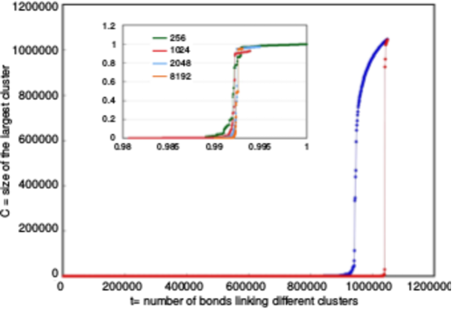
A way to distinguish the difference in the transition between the regular and the PR percolation is by accounting for two different times: the time at which , and the time at which [9]. By calling , Achlioptas, D’Souza, and Spencer found that for unbiased growth of ER networks, while for the PR growth, and therefore the two transitions are qualitatively different [9]. Ziff measured the same quantities for regular and PR growths on square lattices with different sizes, and also found that the relationship between and is quite different. For regular percolation, was found, while for the PR model [33]. Notice that as for both the PR and random growth models. However, it was later discovered that, with a different criterion for the upper end of the gap (say ), then one would find that as for the random growth, while still for the PR model [35].
Kim et al. considered the formation of single-walled nano-tube bundles with uniform diameter [45]. Except for the growing process, they also measured the changes in the order parameter during the stick removal process, and found that a hysteresis exists. This result clearly shows that the transition of the stick system with cluster repulsion is discontinuous. AP in such a nano-stick system is defined as follows [45]:
-
(I)
One first places two sticks and at random positions with random orientations.
-
(II)
Then one lets () be the sizes of the clusters which would merge into a bigger one of size () by the placement of the stick (). Here, the size is defined by the number of sticks in the cluster. A PR is adopted by calculating the products:
(1) -
(III)
If () then the stick () is kept and the stick () is removed. Processes (II) and (III) favor the connection between small clusters, which suppresses the growth of larger ones.
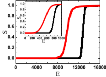
An order parameter is introduced to describe the probability that a stick belongs to a spanning (largest) cluster [45],
| (2) |
where is the number of sticks in the spanning cluster, and is the total number of sticks placed in a given square. In general, EP is marked by the existence of a jump in the order parameter at the critical connecting probability . For convenience, this probability is here replaced by the total number of sticks [45]. Although these two approaches are similar, some differences between the variables and have to be noticed. For the former, is a state variable and is thus independent of the evolutionary process. A small increase of will result in an increase of approximately new sticks, which is enough to induce a significant increase of . For the latter, instead, is an evolutionary variable and is equivalent to the time . That is, will increase one by one, and this will result in a gradual increase of . In this sense, we cannot expect a jumping of in Eq. (2) at the critical point, but only a fast or explosive growing of .
A first-order like phase transition is usually accompanied with a property of history-dependence, i.e. the existence of a hysteresis loop, because of the presence of meta-stable states. Therefore, one of the most generally accepted (and simplest) methods to verify whether or not an observed transition is first-order like is the existence of a hysteresis loop [114, 115]. To measure the hysteresis, one needs to consider both processes of adding and removing sticks. Results are shown in Fig. 6, which clearly manifests the existence of a hysteresis, indicating a first-order like transition.
2.5.2 Site percolation
An alternative mechanism is site percolation [36, 37]. It refers to a situation where, initially, all the sites of a square are empty. During the growing process, sites are sequentially occupied, and two occupied neighboring sites are considered to belong to the same cluster. The AP rule is applied as follows. One chooses two candidates at each time step, and investigates which one of them would lead to the smaller clustering. This one is then kept and the other discarded.
Bastas, Kosmidis, and Argyrakis found that this procedure considerably slows down the emergence of the giant component [36]. Their algorithm for the case of the sum rule proceeds as follows: initially, one starts from an empty lattice and randomly occupies a single site. Then, at each time step, one randomly chooses two unoccupied sites, say and , and calculates the sizes and of the resulting clusters to which and belong, respectively. When (), site is permanently occupied, and site discarded. When , one randomly selects either or and permanently occupies it. With representing the largest cluster at time , the process is repeated until the entire lattice is covered.
Figure 7 shows an illustrative example of the algorithm applied on an square lattice with periodic boundary conditions, where the white (colored) cells correspond to unoccupied (occupied) sites, and where different colors (red, green, gray, and blue) indicate different clusters. In Fig. 7(a) one randomly selects a pair of unoccupied sites (yellow), say and , one at a time, and evaluates the size of the clusters that are formed when and are considered, and , respectively. One finds that and . Therefore, is kept (because it leads to the smaller cluster) and is discarded. The result of this operation is shown in Fig. 7(b).
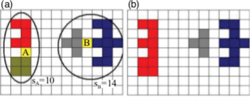
Similarly to the case of bond percolation, one can introduce here an order parameter to track the explosive nature of the transition, which is defined as the ratio of the sites that belong to the largest cluster to the total number of sites in the lattice,
| (3) |
where . By monitoring this quantity, Bastas et al. [36] found an explosive behavior similar to that of Figs. 5 and 6.
Later on, Choi, Yook, and Kim studied the explosive site percolation under AP with a product rule in a 2D square, and also found the existence of a hysteresis loop in the order parameter [37]. The algorithm is similar to the one in Eq. (1) with the word “sticks” replaced by “sites”. The reverse AP process is also the same as in Ref. [45]. The main difference is that in Eq. (1) is now at most , while for bond percolation is always . Choi et al. noticed a qualitative difference in the hysteresis loops between the SR and PR cases. Let represent the area enclosed by for the increasing and decreasing processes on . The SR shows that as [36], while the PR shows that increases when increases and then saturates to a nonzero value [37]. In a 2D lattice, the PR induces a transition whose nature is completely different from that induced by the SR, as the percolation transition caused by the PR is discontinuous.
2.6 Mechanisms for explosive percolation
The first studies and predictions on EP (with Achlioptas processes on top of ER random networks) were mainly based on numerical simulations [9]. Subsequent studies, however, tried to dwell more deeply upon the generation mechanisms for the observed explosiveness in the transition.
2.6.1 Powder keg
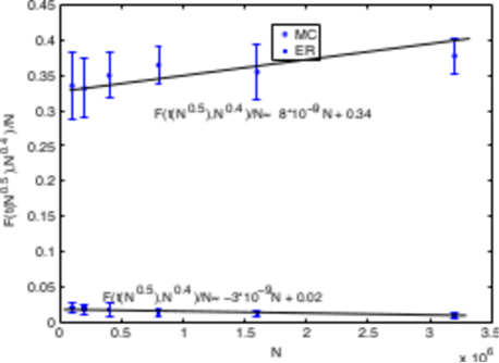
First, Friedman and Landsberg tried to relate EP with a sort of “powder keg” mechanism taking place immediately before the explosive transition in ER-type models [52]. More specifically, before the onset of the transition, a fixed non-zero fraction of nodes in a small-sized cluster constitutes a “powder keg”. Let therefore be the number of nodes in clusters of size after the addition of the -th edge. In AP processes with sum rules, one finds that the powder keg
| (4) |
approaches a non-zero constant in the large limit for some , and . In other words, at time (which is the beginning of the phase transition) a fixed non-zero fraction of nodes are contained in small clusters with sizes ranging from to . This set is termed as the powder keg, and has a size approaching a non-zero constant in the large -limit under the AP rule, while the powder keg is empty in the large limit for ER rules. Such a conclusion was based on a linear regression of data, comparing the size of the powder keg (estimated numerically) and the system size , as shown in Fig. 8 for and .
Although each individual cluster in this set of small-sized clusters contains only a vanishing small fraction of nodes, if taken together these nodes are ignitable and collectively enable an explosive transition. Based on identified powder keg of appropriate sizes, a heuristic criterion has been proposed to predict whether or not a given random network will display EP. In particular, it is conjectured that any “reasonable” network model for which the probability of creating a cluster of size at time is proportional to with will produce a powder keg. A more simplified criterion based on powder keg has been proposed in Ref. [56], which concludes that, under general conditions, a percolation process will be explosive if the mean number of nodes per cluster diverges at the onset of the phase transition in the thermodynamic limit.
2.6.2 Suppression principle
The original model of AP essentially identifies the dynamics that prevents the creation of a giant cluster by choosing one edge from a given number of randomly selected potential candidates [9]. The following two ingredients are sufficient for obtaining an explosive transition [77]: (i) the size of all growing clusters should be kept approximately the same, and (ii) the merging bonds should dominate with respect to the redundant bonds. The term “merging bonds” indicates those edges that connect vertices in distinct clusters, while “redundant bonds” are edges connecting vertices in the same cluster, as shown in Fig. 9. These two conditions are sufficient for obtaining a first-order like transition in a growth process where bonds are included one by one. More precisely, merging bonds must be introduced with much higher probability than redundant ones.
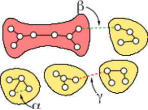
By defining a Hamiltonian of a graph that includes the two ingredients, one can explicitly study the distinct roles of merging and redundant bonds. reads as
| (5) |
where the sum is over the entire set of clusters , is the number of vertices in cluster , and is the number of redundant bonds added to the cluster. The parameter controls the probability of redundant bonds to be added to the system. For small values of , redundant bonds are favored over merging bonds, and one might expect that a new merging bond will be included only after the addition of all possible redundant bonds. The situation becomes different when is large, and redundant bonds are not included. By tuning the parameter in Eq. (5) from small to large values (from to ), a change from a slow continuous growth to a sharp transition is observed, as shown in Fig. 10, which reports the fraction occupied by the largest cluster vs. the average connectivity .
The same idea is also referred to as the suppression principle (SP) [47]. As schematically reported in Fig. 11, one first classifies the types of edge candidate pairs and as follows: (i) both and connects clusters of potentially different sizes. Clusters of sizes and are connected by the edge , and clusters of sizes and are connected by the edge ; (ii) one edge (say, ) is an intra-cluster edge (in a cluster of size ), while the other edge () is an inter-cluster edge and connects the two clusters of sizes and ; and (iii) both and are intra-cluster edges in either the same cluster or two distinct clusters.
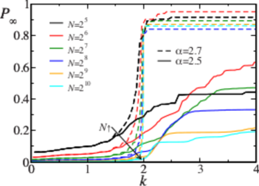
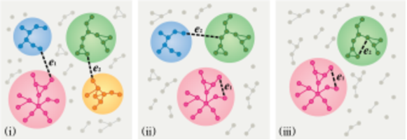
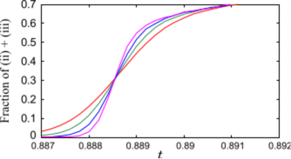
Based on the above classification, several variants of dynamic rules have been proposed to determine whether the SP is fulfilled. In a class of models (models of type A) one edge is an intra-cluster edge (cases (ii) or (iii)). In another class (models of type B) when the case (ii) is considered and the intra-cluster edge is selected, so that the cluster size does not increase. When the two potential edges are both intra-cluster edges [case (iii)], one of them is randomly selected. In a third class of models (models of type C), the dynamics proceeds via only inter-cluster connections [case (i)]. Models of type C may be regarded to be the same as models of type B, because the clusters do not grow when the intra-cluster edge is selected. The difference between type B and type C models is that time advances in type B model but not in type C model. Type A models can fail to follow the SP. For instance, when , , and , the edge is selected in type A models, and therefore, the size of the resulted cluster is . On the other hand, if edge is selected, then none of the clusters would increase in size. As time approaches the percolation threshold, intra-cluster edges can be selected more frequently, which leads to a more frequent failure of suppression principles, as shown in Fig. 12.
In addition, based on the same classification, a fundamental difference between the product and sum rules can be identified. In particular, the PR may not satisfy the suppression principle. A simple example of two inter-cluster connections can be considered, in which , , , and . The product of the two inter-clusters is respectively and , and therefore, edge is added to the system. However, the resulting cluster size is in this case, which is larger than the resulting size when is added. Therefore the SP is not fulfilled.
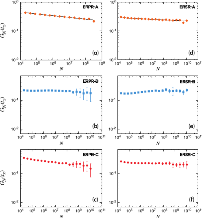
The SR may remove the drawback inherent to the PR, yielding discontinuous percolation transition as observed numerically [47]. To evaluate the discontinuity of the transition, the following two criteria have been proposed: (a) the values remain finite as , where the time is regarded as the transition point in the thermodynamic limit, and represents the components at time ; (b) the tangent of the curve of with respect to at diverges as increases. More specifically, as shown in Fig. 13(a)-(c), for all models with product rules, decreases with increasing in the whole considered range, suggesting that in the limit . Furthermore, when the SR is implemented in type A models, a similar convergence of in the limit is observed in Fig. 13(d). This indicates that these cases violate the SP, and lead to a continuous percolation transition. However, when the SR is implemented in type B and C models, the asymptotic values of look relatively flat, yielding discontinuous percolation transitions within the range of the numerical data (see Figs. 13(e)-(f)).
The original dCDGM model [11] does not follow the suppression principle, because it does not take into account the natural choice of intra-cluster edges. The selection of an intra-cluster edge becomes actually more and more frequent as time approaches the percolation point, and this yields a continuous transition. However, once the dCDGM model is properly modified, discontinuities in the transitions can be observed. The suppression principle plays a fundamental role in achieving discontinuous percolation on random graphs, inter-dependent networks [95, 100], adaptive networks [32, 116], and fractal networks [103].
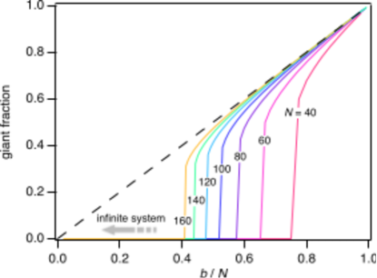
For a finite size system, suppressive rules are not a necessary condition for the sharpness of the transition at the percolation point [104]. Rather, a finite size system with aggressive tendency to form a giant cluster may exhibit an instability that is relieved through an abrupt and discontinuous transition to the stable branch. Although the Author of Ref. [104] has tracked analytically such an abrupt transition to percolation, it is worth noticing that discontinuity is especially pronounced in small size networks, but it disappears when the size tends to infinite, as shown in Fig. 14. This suggests that in the thermodynamic limit the system actually shows a continuous transition to percolation, a point which will be further discussed in Section 2.7.
Generally speaking, the idea of AP is that of choosing the best among randomly given multiple options, in order to avoid the formation of a certain target pattern [13]. In Ref. [86] the spanning cluster rather than the giant cluster is chosen as the target pattern. Such a latter choice enables one to determine analytically the order of the EP transition in the thermodynamic limit, and in particular for percolation in a Euclidean space. Spanning cluster avoiding models feature either discontinuous or continuous percolation transition, depending on the dimension of the Euclidean space in which the dynamics is implemented. More specifically, the EP is continuous or discontinuous if , and it is always continuous if (where is the spatial dimension), this way explaining some of the confusing and contradictory behavior previously observed [87].
2.6.3 Growth by overtaking
The growth by dominant overtaking has been interpreted as the mechanism responsible for the discontinuous percolation transition of the Bohman-Frieze-Wormald (BFW) model [73]. More specifically, the BFW model has been extended to the case where various constraints exist on the occupation of competitive edges. Such a simple stochastic graph evolution examines only one edge at a time, which leads to a discontinuous transition provided the control parameter is small enough. The overtaking mechanism means that the size of the largest component does not change by direct growth, but it changes when two smaller components merge and become the new largest component. On the other hand, a continuous transition appears if is large enough to allow substantial direct growth of the giant component. Notice that the BFW model has been originally proposed to study discontinuous percolation with multiple giant clusters in Ref. [70], and was further studied on finite dimensional square, simple-cubic lattices, and SF networks obtaining similar results [71, 72, 117, 118]. Furthermore, in the generalized BFW model, it has been shown that the emergence of global connectivity is announced by microscopic transitions of the largest component [74].
2.6.4 Recursive and hierarchical structures
Networks with a recursive and hierarchical structure induce explosive percolation dynamics as well, although the formation of an extensive cluster is restricted to ordinary (uncorrelated) and random bond addition [103]. This suggests that a hierarchy of SW bonds grafted onto a one-dimensional lattice results in an EP transition, even if bonds are added sequentially in an uncorrelated manner.
2.7 Debates on explosive percolation
The results of Ref. [9] have triggered a big debate in the community, aiming at definitely clarifying whether the observed transition are discontinuous or not. In equilibrium systems, discontinuous phase transitions are usually identified as first-order transitions, while its counterpart of continuous transitions are called second-order transitions. However, the term of “explosive percolation transition” was solely based on the numerical evidence of a jump (a sort of discontinuity from a visualization perspective) in the order parameter at the critical transition point. Therefore, all numerical results in Refs. [33, 48, 49, 52, 34, 62, 44, 35, 56, 80] initially focused on searching for the existence of such a discrete jump.
2.7.1 Finite-size scaling theory
While the existence of a discontinuous jump in EP was confirmed since the earliest studies on the subject, most other properties of a first-order transition (like cooperation, phase coexistence, and nucleation [12]) had to be proved. From the physical point of view, the competitive choice of a new link suppresses the formation of large clusters, which yields the threshold value significantly delayed in comparison to random percolation. Therefore, the competitive percolation transition can be extremely abrupt with a large (seemingly discontinuous) jump in the connectivity of the graph. Although systems of rather large sizes (i.e., tens of billions of nodes) are used in the original AP model, the heuristic arguments of discontinuity at the percolation transition disappears in the thermodynamic limit. Therefore, the term “explosive” refers here to the unusual feature which distinguishes the critical behavior of the AP from both ordinary and truly discontinuous models [51].
Finite-size scaling theory is useful for characterizing phase transitions [119, 120]. Traditionally, the percolation transition has been conceived as a typical continuous phase transition displaying a power law size distribution, and a set of standard scaling properties. Therefore, a percolation transition is continuous if one finds the signature of power law distribution of component sizes. In contrast, it is discontinuous if a power law distribution does not exist.
The first systematic analysis of cluster size distributions for AP by finite-size scaling theory has been reported in Ref. [34], including lattices, random, and scale free networks. For continuous phase transitions, every variable of interest near the percolation threshold (critical average connectivity of the network in the limit of infinite size) is scale independent, due to the infinite correlation length of the system at , so it has a power-law form
| (6) |
where is a critical exponent. On a system of a finite size , the scaling of the variable is normalized as follows:
| (7) |
where is another critical exponent, and is a universal function. Both critical exponents and are associated with the magnetization and the correlation length, respectively. For , the variable shows a simple scaling , which can be used to deduce by examining several systems of different sizes. Furthermore, if are known, the plot of as a function of yields the universal function , which does not depend on .
In the case of percolation, one chooses to be the average value of the order parameter , which measures the relative size of the largest connected component with respect to the total system size (i.e., the number of nodes belonging to the largest connected component divided by ), and which is also called “percolation strength” [34, 11, 12].
The identification of the percolation threshold is performed in several independent ways [34]. One way is to plot the order parameter as a function of the system size , for a given value of . A correct value of the percolation threshold can be determined by finding the value of which yields the best power-law fit. The second method consists in using the scaling of the pseudo-critical points , defined as
| (8) |
where is a constant to be determined from the fit, together with the other critical parameters and . The pseudo-critical value can be simply obtained by the monitoring positions of the peaks of at different system sizes .
An alternative quantity that can be adopted as variable in Eq. (7) is the susceptibility, which again can have two slightly different definitions. The first is to consider the mean cluster size , where stands for the number of clusters of size per node. The sums run over all possible values of , except for the one of the largest cluster [34, 44]. The second definition is obtained by considering the amplitude of the fluctuations of the order parameter , i.e. [49, 44]. When these susceptibility measures are used, the critical exponent is indicated by , and the scaling ansatz is , where the universal function is different from .
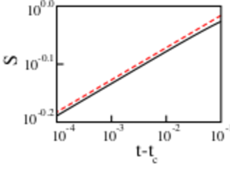
For ER networks, the order parameter starts to be defined at the percolation threshold , and grows with time as , with . For randomly diluted -dimensional lattices, depends on . At , the cluster size distribution (the fraction of finite connected components of nodes) scales as , with . When the transition is discontinuous, the finite size scaling theory does not apply anymore, and the scaling relation of Eq. (7) trivially holds with . The curves of versus do not scale as well, and approaches at increasing faster than a power law.
Simulations of EP performed for AP-type processes reveal power law distributions of cluster sizes as well, resembling the results of continuous percolation transitions. It turns out that this self-contradicting combination of discontinuity and scaling has made EP one of the most challenging and urgent issues. The first contradicting result has been reported in Ref. [11], which concludes that EP is actually continuous for a modified version of the AP (the dCDGM model), and analytically derives the critical scaling relations based on numerical observations of power-law critical distribution of cluster sizes, with a unique small critical exponent . The numerical simulation for a very large system ( nodes) shows a pronounced power law regime, which indicates a continuous transition (see Fig. 15). The small exponent makes the transition so sharp that it is almost indistinguishable from a discontinuous one.
Further systematic analysis of finite size scaling was performed for four Achlioptas-type processes [12], showing unusual behaviors with non-analytic scaling functions which demonstrate that AP-like percolation transitions are indeed continuous. More specifically, Ref. [12] characterized the phase transitions in terms of the distribution of the order parameter , where is the control parameter and is the system’s size. The distribution at criticality scales, for continuous transitions, as
| (9) |
where is a universal function. This equation is directly related to the finite size scaling relation of Eq. (7). For a continuous phase transition, the universal function might be double peaked, but then, as , the dip between two peaks usually does not deepen and the horizontal distance between them shrinks to zero, so that becomes single humped. In contrast, in typical first-order transitions, is double peaked with a deepening valley between the two peaks. Furthermore, the distance between the peaks tends to be equal to the value of the jump observed in the order parameter .
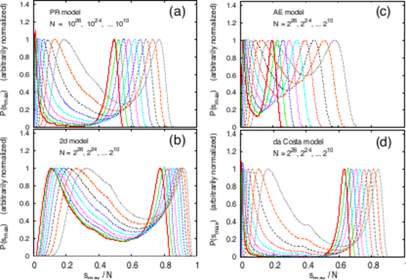
The results are shown in Fig. 16. Notice that, while the two peaks seem to indicate an indeed explosive character of the percolation transition, they do not yet prove that EP is discontinuous. For the latter, one must also show that the distance between the peaks does not vanish for . It turns out that the valley between the peaks deepens with increasing in all cases, but at the same time both peaks shit to the left (see Fig. 16). Ref. [12] also confirms that the critical exponent is rather small. Furthermore, the distance between the peaks decreases for large . As a matter of fact, one may extract information on the continuous transition from the depth and position of the valley [121].
In the original AP model with the PR on a complete graph, a careful finite size scaling analysis has shown that EP transition is indeed continuous in the thermodynamic limit [107]. For percolation processes, the main question is whether the gap () vanishes or not. To this end, the strategy consists in the following steps: (i) the information above the transition point is used to set up lower and upper pseudo-transition points, and . This provides an easy way to find , since one would expect that both pseudo-transition points converge to as . (ii) The upper bound for the size increase of the largest cluster between and is found, namely . This is equivalent to consider the gap of the order parameter between the two pseudo-transition points . (iii) Such an upper bound turns out to be sub-linear in for a continuous percolation transition, and therefore the investigation of the cluster size distribution leads to conclude that the explosive percolation transition is indeed continuous.
Other developments regarding the application of finite size scaling analysis to EP can be found in Refs. [44, 39]. For a wide set of representative AP models, an exhaustive investigation has been conducted in Ref. [65], where the full set of scaling relations between critical exponents was found, together with the scaling functions and the upper critical dimension.
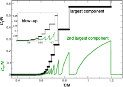
2.7.2 Discontinuity of the transition
Finally, the continuity of the EP transition has been rigorously proven in Ref. [13], which indeed mathematically demonstrated that continuity is an essential feature of all mean-field AP models, and of a wide range of their variants. For instance, any competitive rule based on picking a fixed number of edges would lead to a continuous transition. Furthermore, it is shown that the order parameter of the AP percolation models has random fluctuations that do not disappear in the thermodynamic limit [60]. On the other hand, a discontinuous phase transition may appear if the number of nodes sampled grows with the network size [75]. Discontinuous transitions are observed in some models (such as, for instance, the BFW model [70]), and in a hierarchy of SW random bonds model [103]. Notice that the results of Ref. [13] do not imply that the percolation transition at is characterized by a power law divergence of the order parameter, nor they mean that a globally continuous transition cannot be entangled by multiple discontinuous transitions. For instance, for certain -vertex rules, the continuous percolation transition can have an incomplete devil’s staircase with multiple discontinuous steps in the vicinity of [59], as reported in Fig. 17.
2.7.3 Irreversibility of the transition
The last point to be discussed is that EP processes are irreversible, in contrast to traditional continuous percolation. In the latter case indeed, one can reach any state either adding or removing connections. For EP, instead, only adding links makes sense, while the inverse process is impossible [11]. This argument suggests that any efforts in searching hysteresis behavior in EP would fail. Typically, hysteresis is considered to be a necessary condition of a first-order phase transition. For AP processes on 2D square lattices of finite size, hysteresis behavior between the forward (adding edges) and the reverse (removing edges) processes has been numerically observed in Ref. [36]. However, the hysteretic area tends to 0 in the thermodynamic limit, which indirectly shows that the product rule of EP processes generates a continuous transition. In a different model embedded in a Euclidean space (that chooses the spanning cluster instead of the giant cluster as the target pattern) a hysteretic loop has been observed in discontinuous percolation transitions [86].
3 Synchronization as a continuous phase transition
3.1 Introduction and historical overview
Synchronization is possibly one of the most ubiquitous natural phenomena. There, inanimate or living systems [122] tend to adjust their own rhythms due to an existing coupling interaction, or a driving force. It was known for few centuries that two pendulum clocks can synchronize when hanging from the same piece of wood. Since then, synchronization has captivated the interest of scientists and, nowadays, it is investigated in fields as diverse as natural and social sciences [8], or engineering [4]. Popular examples of systems exhibiting synchrony are: birds flocking together, fishes swimming in schools, male fireflies flashing together, people clapping in unison after a performance, pacemaker cells in the heart, -cells in a pancreatic islet, and neurons in the brain. For comprehensive reviews providing the detailed description of synchronization phenomena we address the reader to Refs. [8, 5, 6, 123, 7].
When the coupled systems are oscillators, the fate of synchronization always depends on two ingredients: i) the frequency detuning (the more alike the systems are, the better is synchronization), and ii) the coupling pattern (i.e. the strength, the network topology, the output function) through which the network’s units communicate. It is not sufficient, indeed, that two systems are alike, it is also necessary that the information exchanged between the systems is of good quality to allow them to synchronize [124, 125, 126].
As a coupling strength increases, a transition from an incoherent to a coherent phase takes place generically at a critical value, where the elements follow the same dynamical behavior. The nature of such a macroscopic rhythm can be described by an order parameter (in analogy with phase transitions in statistical mechanics [127]). As first pointed out by Winfree [128], in most of the cases the transition is second-order like, with the order parameter exhibiting power-law divergences at the onset of the synchronization. Figure 18 shows an example of such a transition in the case of -cells within a pancreatic islet, which burst all in synchrony, and therefore produce a coordinated insulin release in response to glucose [129].
Abrupt (discontinuous) transitions to synchrony have been recently reported [23, 14, 130] where an infinitesimal variation of the coupling strength gives rise to a macroscopic synchronous phase exhibiting hysteresis, a feature observed in theoretical models of coupled Josephson junctions [131], as well as in more complex coupled oscillators models [132, 133, 134, 130, 135, 136]. These abrupt transitions will be the object of the next Chapter, whereas the present Chapter has the aim of reviewing the classical works on synchronization, the synchronization types and the main indicators and models used to describe the spontaneous emergence of ordered states.
3.2 Synchronization of two coupled dynamical systems
The case of two coupled dynamical systems constitutes the building block for the later study of networked systems. The problem is properly framed by considering each systems as described by a -dimensional () vector (). In general, the equation of motion is given by:
| (10) |
where . Each unit evolves according to the velocity field , and can reach either a stable fixed point, or a limit cycle, or a chaotic attractor [122, 137].
Equation (10) accounts for the general framework in which the two systems can be of different nature, have different dimensions, and the interaction can be described by any generic function of their dynamical states. However, in order to allow an analytical treatment of the problem, the autonomous dynamics is assumed to be independent from the interaction between the units, and a particular form of interaction has to be assumed. We here focus on the case in which each unit is coupled to a linear superposition of the outputs, and the interaction is symmetrical:
| (11) |
where represents the coupling strength, and are vectorial functions, and is a matrix satisfying the rules of a diffusive coupling (). For two units, one has therefore .
3.2.1 Complete synchronization
If the systems are identical (), the synchronization is realized by the equality of the state variables as they evolve in time (), and is termed as complete (or identical or full, or conventional) synchronization [138, 139, 5].
Complete synchronization (CS), , is a threshold phenomenon and occurs beyond a critical value of the coupling strength. CS can be observed by monitoring the mean synchronization error, defined as:
| (12) |
i.e., the averaged distance to the synchronization manifold .
One of the most popular approaches to assess the stability of CS is the master stability function (MSF) method, introduced for arrays of coupled systems in Ref. [140]. The MSF is the largest Lyapunov exponent transverse to the synchronization manifold, and measures the exponential rate at which any infinitesimal perturbation decays or grows. Therefore, a necessary condition for CS to occur is that the MSF is negative.
3.2.2 Phase synchronization
Real systems, however, are not identical, and they are subjected in general to noise or parameter mismatch preventing CS. Weaker forms of synchronization exists, where correlation or equality of the two systems are limited to proper subsets, or functions, of the variables.
When two periodic oscillators are coupled, for instance, synchronization is observed as the entrainment of their phases and frequencies. When the systems are uncoupled, the two stable limit cycles are described by two phases whose dynamics are governed by their respective natural frequencies and as , which in general are incommensurate (). Phase locking means here that the phase difference () is bounded beyond a certain coupling strength, and the corresponding instantaneous frequencies are locked, i.e.,
The onset of synchronization is therefore a transition from a quasi-periodic motion (with two incommensurate frequencies) to a motion with a single frequency, and can be characterized by means of families of Arnold tongues [141], i.e. synchronization regions where the relationship holds. Inside those regions, the oscillators mutually adjust their frequencies until attaining the relation , with the resulting synchronization frequency depending on the initial frequency detuning . Moving away from the border of an Arnold tongue, the phase difference uniformly grows in time.
Phase synchronization has been later extended to chaotic oscillators [142]. When the chaotic oscillators have a well defined center of rotation, as it is the case of phase coherent systems, the instantaneous phase can be reliably calculated by means of few mathematical techniques [5]. The mean square displacement of the phase linearly diffuses in time (with a very small diffusion constant), due to the pronounced variations of the amplitude modulating the rotations. As two phase coherent chaotic oscillators are coupled, a transition from a non-synchronous regime (where the phase difference linearly grows in time) to a synchronous regime (where the phase difference is bounded and the mean frequencies are equal) occurs.
When instead the two chaotic oscillators are not phase coherent (and exhibit a broad distribution of time scales), phases do not fully synchronize, and synchronization episodes are interrupted by intermittent phase slips (jumps of in the phase difference). Such a latter phenomenon has been called imperfect phase synchronization [143] and it has been observed experimentally in an electronic circuit representing a forced Lorenz system [144].
3.2.3 Lag, anticipated, relay and generalized synchronization
After the setting of a phase synchronization, intermediate values of the coupling strength drive the systems into a stronger degree of synchronization, where also amplitudes start to become correlated. The resulting regime corresponds to the dynamics of one of the oscillators which lags (in lag synchronization [145]) or leads (in anticipated synchronization [146, 147]) the dynamics of the other. Lag synchronization was first shown in symmetrically coupled nonidentical oscillators [145], and the time shifting between one and the other state’s variable was detected as the minimum of a time dependent similarity function.
The existence of this achronal synchronization in mutually delayed-coupled oscillators has been observed in laser systems [148], and studied theoretically in Ref. [149]. It is possible also to have two completely synchronized chaotic units in the presence of a delayed coupling, phenomenon known as zero-lag or isochronal synchronization [150, 151]. Such a regime can be achieved via a self-feedback in both coupled units [152, 153], or via an indirect coupling through a relay [154], or through a third driving unit [155, 156, 157], or when multiple coupling delay times are used [158].
In the so called relay systems, two units achieve CS as a result of an indirect coupling through a third system acting as a relay. Experimental evidence of relay synchronization has been obtained with lasers [150, 159, 154] and electronic circuits [155, 157]. Relay synchronization has been further used as a method for chaos-based communications [153, 156, 160, 151], as well as a synchronizing mechanism among remote neuronal resources [161, 162, 163].
Anticipated synchronization, on the other hand, may occur in systems coupled in a drive-response configuration, and it relies on the use of time delay lines in the dynamics of the slave system. It has been studied theoretically and numerically in different contexts including dissipative chaotic flows [146, 147, 164], chaotic maps [165], excitable spiking neurons [166, 167, 168, 169], inertial ratchets [170], and complex Ginzburg-Landau equation [171]. Experimentally, it has been observed in electronic circuits [172, 173, 166, 174] and in optical systems [175, 176]. Furthermore, the fact that behavior of one of the oscillator can be forecasted up to time scales larger than those characteristics of the system’s dynamics has been used recently as a method to control and suppress unwanted spikes in excitable systems [177], or to anticipate or suppress extreme desynchronization events [174].
A further form of synchronization, called generalized synchronization [178, 179], involves the existence of a time-independent functional relationship between the states of the two coupled units (typically nonidentical), such that . Initially, this type of synchronization was found for unidirectional coupling schemes and proved experimentally by means of the auxiliary system method [180, 181]. Recently, generalized synchronization has been reported also for bidirectionally coupled oscillators [182, 183, 184]. In particular, Gutiérrez et al. provided evidence that relay synchronization corresponds in fact to the setting of generalized synchronization between the relay and the outer units [184].
Finally, for very large coupling or parameter mismatches a counterintuitive phenomenon may emerge that suppresses the oscillations, termed as oscillation quenching. Such a phenomenon can be manifested in two distinct ways, whose origin is structurally different: amplitude death and oscillation death. In the former case, the suppression of oscillations results in the existence of a homogeneous steady state, in the latter a homogeneous unstable steady state splits, giving rise to an inhomogeneous state with two coexisting steady states. Refs. [185, 186] are two very recent reviews on the subject.
3.3 Synchronization in ensembles of coupled systems
The scenario described in Section 3.2 can be generalized to ensembles of spatially ordered oscillators, coupled (either locally or globally) in chains and lattices, as well as to spatially extended oscillatory media. Synchronization in these contexts, indeed, is very relevant for the study of cooperative behavior in many physical [187], biological [128, 188, 189] and chemical systems [23, 190, 191, 192]. For a review, the reader is addressed to the books in Refs. [8] and [193].
3.3.1 Identical systems
Assemblies of coupled identical systems can exhibit non trivial synchronization patterns. Precisely, two types of synchronous behavior can be produced: full or global synchronization where all elements evolve identically in time, and partial or cluster synchronization in which groups of mutually synchronized systems with different synchronization patterns emerge. The specific scenario that is produced (and its features) depends on many factors: the number of units, the way they are mutually coupled, and the initial and boundary conditions.
Formally, the coupling conditions may be classified as local (by setting in Eq. (11) for , and zero otherwise), global ( ), and non-local (, where is a decreasing function of the distance between oscillators and ).
From now on, we will focus mostly on the case in which each unit of the ensemble is an oscillator. In such a case, the amplitude of the mean field is taken as an indicator of the onset of coherence. If all the frequencies in the ensemble are different, then the instantaneous phases are uniformly distributed in the interval , and the mean field vanishes. If instead some of the oscillators are locked to the same frequency, the vectors associated to their phases sum up coherently in the unit circle, and the mean field is non-zero. A weaker condition of synchronization is the coincidence of the averaged frequencies .
Ensembles of locally identical coupled systems have been studied through chaotic maps [194, 195, 196] and flows [197, 198, 179, 199, 200], and limit-cycle oscillators. An example is the complex Ginzburg-Landau equation [201, 202] which represents the normal form of an Hopf bifurcation, and describes a wide variety of wave phenomena, including phase turbulence (spatiotemporal chaos), plane waves, targets and spirals in which oscillations are synchronized [201]. As for globally coupled systems, the main studies have concerned chaotic maps [203, 204, 205, 206] and flows [197, 207, 208], rotators with diffusive [209, 210, 136, 211] or pulsed [212, 213, 214] coupling. Experiments instead have been conducted with chaotic electrochemical oscillators [215].
Regardless on the specific framework that is considered, a transition is generically found from global (at large coupling) to cluster (at intermediate coupling) synchronization. Detailed analysis of the mechanisms determining the loss of stability of the global coherent state into a hierarchical cluster dynamics can be found in Refs. [205, 206], while Ref. [216] studies the destabilization of the synchronous state for increasing coupling due to the so called short-wavelength bifurcation. Ref. [204] analyzed the cluster structure emerging in a system of randomly coupled identical maps, as a function of the average connectivity.
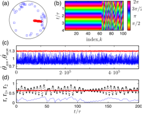
3.3.2 Chimera states
Together with the emergence of clustered synchronous patterns, an even more surprising phenomenon is the coexistence of clusters of coherent and incoherent phases in ensembles of identical oscillators, which was termed as chimera state by Abrams et al. in 2004 [217]. As an example, Fig. 19 shows the coexistence of a synchronized cluster of 64 oscillators and a cloud of 36 asynchronous ones, which emerge in a homogeneous ensemble of globally coupled oscillators, due to an internal delayed feedback in individual units [211]. First noticed by Battogtokh and Kuramoto [218], the breakdown of spatial coherence in the presence of non-local interaction has been reported theoretically [219, 217, 220, 221, 222], and numerically [223, 224]. Experimental evidences of chimera states have been obtained in chemical [225, 226], optical [227] and mechanical [228] systems. For instance, in Fig. 20, a chimera state is observed in a photosensitive Belousov-Zhabotinsky reaction, in which the catalyst is loaded onto ion-exchange oscillatory particles. The oscillatory particles are divided into two groups of equal size ( and ), with each member of group experiencing the feedback light intensity :
being and . is the mean intensity in group , and are the intra and inter-group coupling coefficients, is a normalized background light intensity, and is the measured intensity scaled from to . The delay plays the role of the phase frustration term used in the model by Abrams et al. [217]. With such a coupling scheme, group remains fully synchronized, while can exhibit three basic states: fully synchronized (Fig. 20(a)), cluster ( in Fig. 20(b)) and the unsynchronized chimera (Fig. 20(c)). Panel (d) shows the behaviors found at different intra- and inter-group coupling strengths, under the setting of and .
Coexistence of coherence and incoherence has also been observed in networks of coupled nonidentical phase oscillators [229, 230], and in globally coupled populations of identical oscillators [231] with internal delayed feedback [219, 211]. A recent review on the subject [232] gives a comprehensive history and overview on chimera states.
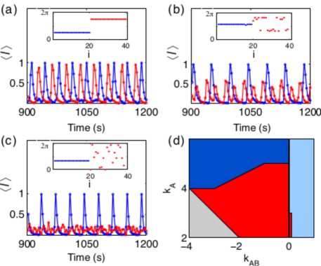
3.3.3 Non-identical systems
Real-world systems often feature noise and various degrees of heterogeneity. Therefore, synchronization phenomena have been explored in large ensembles of interacting non-identical oscillators [23].
The same routes of two coupled oscillators can also be explored for ensembles of locally or globally coupled (periodic or chaotic) systems. As long as oscillators are phase coherent, there is no qualitative difference between periodic and chaotic case [233, 234, 235], with the exception that chaotic assemblies can display phase synchronization while their amplitudes remain uncorrelated.
The transition to synchronization in chains of periodic [236, 234] and phase coherent chaotic [233] oscillators with different frequencies can occur in a soft or a hard way, depending on the frequency mismatch of the oscillators. Namely, for a linear distribution with a small mismatch, the transition is smooth, while for large mismatches the transition is characterized by an abrupt formation of clusters with phase slips between them and whose size is increasing with the coupling. In the case of randomly distributed frequencies, only the hard transition is possible, and the onset of synchronization appears for lower values of the coupling.
3.3.4 The Kuramoto model
Despite the peculiarity of the system under study, a large population of weakly interacting oscillators can be described by considering their phases, and assuming a homogeneous interaction among them. With such an assumption, Kuramoto formulated his celebrated equation [187, 23] (based on the previous Winfree’s works with phase models [128]) which transforms Eq. (11) into a mathematically tractable one.
The Kuramoto model [187, 23] considers a system of oscillators having natural frequencies distributed according to a probability density which (for the time being) is uni-modal and symmetric around its mean frequency . The instantaneous phases obey the following equations:
| (13) |
where the normalization constant ensures the boundedness of the coupling term in the thermodynamic limit . A transition to synchronization occurs for values of the coupling above a critical threshold , which depends on the distribution . A motivating survey of the Kuramoto model is offered in Ref. [237]. Tutorials and reviews of the main achievements on the Kuramoto model can be found in Refs. [238, 239, 240].
The monitoring of the synchronization onset is performed by introducing a complex mean field of the population, known as the order parameter [187]
| (14) |
Equation (14) is the vector centroid of all oscillators represented as points in the unit circle. is the average phase, and its modulus, which implies and . measures the level of coherence in the population: if the population is synchronized, and if the points are uniformly distributed in the unit circle.
Using the parameters and , Eq. (13) can be rewritten as
| (15) |
Now, the dynamics of each oscillator is implicitly coupled to all the others through the mean field in a positive feedback way: the more coherent is the population, the larger is and the more effective is the coupling strength , which drives therefore more and more oscillators into the synchronization cluster. The threshold value can be derived by self consistency conditions applied to Eq. (15). If one assumes a priori a solution where is constant and is rotating at a constant frequency (), then Eq. (15) can be expressed as a function of the angle using a rotating reference frame at frequency :
| (16) |
The scalar vector field for exhibits a saddle-node bifurcation at or . If , the solution is stable, and oscillators are locked to the mean frequency . The oscillators instead with are uniformly spread around the unit circle.
A rigorous analysis of Eq. (16) has been performed in Refs. [237, 238]. Here we just highlight the main steps in such an analysis. By introducing the probability density function , the fraction of oscillators lying within the arc with natural frequencies is
and the order parameter can be expressed as:
| (17) |
must obey the continuity equation
| (18) |
where is the angular velocity of a given oscillator with phase (in the co-rotating frame) and natural frequency . One obtains therefore the following self-consistency condition
| (19) |
The saddle-node bifurcation manifests as a phase transition from the incoherent state (at with density ) to the partially synchronized state (with ) characterized by a group of phase oscillators rotating in unison at (those whose frequencies obey ), while the remaining ones are rotating incoherently. These solutions satisfy
| (20) |
By expanding the integrand in a Taylor series, one finds that the amplitude of the mean field (at the onset of synchronization) is given by
| (21) |
with
| (22) |
Therefore, the transition is continuous and the order parameter behaves (in the limits ) as
| (23) |
which resembles a continuous second-order phase transition characterized by the critical exponent .
Finally, exploiting the extensive symmetries of the continuum-limit model (17)-(18), Ott and Antonsen derived an exact reduction to a finite set of nonlinear differential equations for the evolution of the order parameter [241, 242]. This latter approach has been used in several recent studies [243, 229, 221, 244].
3.4 Synchronization in complex networks
Units in the ensemble may, however, interact through specific coupling patterns (or connection topologies) which can be conveniently encoded in an interaction network. The seminal paper by Watts and Strogatz [245] proved that the connection topology of networks can be organized in between a regular and a random architecture, and that such a topological arrangement (called SW property) endows the system with enhanced synchronizability. Since then, a flurry of studies has been focused on synchronization in complex networks, and the reader is here addressed to a series of classic [246, 247, 248] and recent [239, 249] reviews on the subject.
We here follow the same path of the previous two Sections, and provide a schematic overview of synchronization on networks, for both cases of identical and non-identical oscillators.
3.4.1 Identical systems
Complete, cluster, and chimera states of synchronization have been reported so far in networks of identical flows or maps. As far as complete synchronization is concerned, one of the main research lines has been the investigation on the stability of this state for different network topologies and dynamical functions.
For a generic network of diffusively coupled identical units there are two main approaches to assess the stability of the synchronous state. The first one is the extension of the MSF [140, 250, 251] to complex networks [252], which related the local stability of the synchronization manifold to the spectral properties of the Laplacian matrix associated to the underlying network structure. A comprehensive derivation of this formalism can be found in Ref. [246]. Precisely, the analysis reduces to plot the maximum Lyapunov exponent transverse to the synchronization manifold as a function of a generic coupling parameter which encodes both the local function and the coupling function in Eq. (11). Different choices of local and coupling functions give rises to three possible classes of MSF. For instance, for a bounded MSF (the so called case of class-III MSF), where within a finite interval , the necessary condition for stability can be attained only if , being and the minimal and maximal non-zero eigenvalues of the Laplacian matrix. The interested reader is here referred to Ref. [246] for the complete discussion on the three possible classes of MSF.
The second method is known as the connection graph stability method, and was derived in Ref. [253]. It combines the Lyapunov function approach with graph theoretical reasoning, and provides a bound for the minimum coupling strength needed for synchronization which explicitly depends on the average path length of the coupling graph.
MSF arguments led to the study of the propensity towards synchronization of different topologies regardless on the nature of the coupled dynamical systems. Ref. [254] introduced a family of graphs, called entangled networks, having an extremely homogeneous structure which optimizes synchronizability: degree, node distance, betweenness, and loop distributions are all very narrow. Therefore, synchronization is shown to be affected by the heterogeneity of the degree distribution, clustering, characteristic path length or betweenness.
Reference [252] compared the synchronizability of a SW network against an interpolated ordered ring structure, and a completely random ER graph, as implemented in Ref. [245]. It was shown that SW graphs exhibit better synchronizability than regular and completely random ones, when the system is far from the complete graph limit. In contrast, Ref. [255] showed that the onset and stability of complete synchronization in networks of pulse coupled oscillators (neurons) only depends on the number of inputs a neuron receives regardless on the details of the network topology, as long as the degree distribution is a function. The effect of link directionality in SW networks has been studied in Ref. [256].
Reference [257] further elaborated on the role of heterogeneity, and realized that heterogeneous structures may display very large ratios ( scales with the hub’s degree, i.e. the largest degree in the graph [258]). The fact that heterogeneous networks may be more difficult to synchronize is known as the paradox of heterogeneity [257]. The effect is due to the overloading of the hubs, which may receive independent inputs and may hamper effective communication between oscillators. The paradox stimulated many scientists to explore mechanisms to improve synchronizability, by the implementation of asymmetric weighting procedures. In Refs. [259, 260], enhanced synchronization is obtained by normalizing the coupling to the power of the node degree (i.e. ), while in Ref. [261] the coupling strength between two nodes is re-scaled to the load of the edge connecting them through the edge’s betweenness centrality (i.e. ). Both methods implement an asymmetric arrangement of the coupling, and promote a dominant interaction from the hubs to the non-hubs nodes [262]. This consideration can be straightforwardly generalized to weighted networks, by showing that synchronizability decreases when the node’s strengths become more heterogeneous [263].
The existence of degree correlations may also affect the propensity for synchronization [264]. In particular, synchronizability is enhanced in disassortative SF networks when smaller nodes drive larger degree ones, while the opposite holds for assortative networks if the hubs are driving the small degree nodes [265, 266]. Synchronizability is therefore enhanced if hubs are strongly inter-connected and drive the nodes with smaller degrees, that is, if the network displays a rich club of large degree nodes.
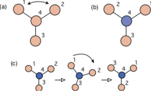
At a more microscopic scale, Ref. [268] showed that the stability of the synchronous states supported by -node and -node motifs is correlated with their relative abundance in undirected networks, while in directed graphs the correlation only holds for some specific motifs. Recently, furthermore, stability of synchronization has been investigated also in relationship with topological criteria which apply to network’s meso-scales [269].
Another extension is that covered by adaptive networks [270], whose structure is shaped by the microscopic organization patterns [263, 271, 272]. To achieve global synchronization, one plausible assumption is to consider that each node tries to synchronize to its neighbors by increasing the coupling strength from them. Inspired by the anti-Hebbian learning rule in neural systems, Ref. [272] studies how the feedback from dynamical synchronization shapes network structure by adding, at every time step, a link between two randomly chosen nodes and with a probability proportional to the rate of their dynamical differences with the mean activity of the network. The evolution of the network spontaneously forms a SF structure with negative degree-degree correlation, a typical feature of technological and biological networks.
On the other hand, Refs. [263, 271] introduced a dynamical feedback principle by means of a nonlinear differential equation for the evolution of the weights which is coupled to the dynamics of the nodes while the connectivity matrix is fixed a priori. In this latter case, when complete synchronization is achieved, the coupling strength becomes weighted and correlated with the topology due to a hierarchical transition to synchronization in heterogeneous networks.
MSF approach has also inspired some pinning control strategy for synchronization [273, 274] where nodes are sequentially perturbed to improve as much as possible the eigenratio of .
More recently, several studies revealed that the symmetry groups in the architecture of complex networks can determine constraints for the appearance (or stability) of a given cluster solution [275]. Cluster synchronization has attracted considerable attention in SW networks of coupled maps [250], chaotic flows [276], synaptically coupled networks of bursting neurons [277] (for diffusively coupled neurons only complete synchronization is possible [255]), or in networks of Stuart-Landau oscillators [278].
In particular, Refs. [267, 279] have studied the emergence and stability of cluster synchronization in networks of coupled oscillators for arbitrary topologies and individual dynamics. Using the tools of computational group theory, Ref. [279] addressed the general case of networks where the intrinsic symmetries are neither ad hoc produced nor easily observed. Figure 21 schematically described a case where a strong relationship exists between symmetry and dynamics: a symmetry (a permutation matrix like a reflection in Fig. 21(b) or rotation in Fig. 21(c)) applied to an adjacency matrix leaves it unchanged (i.e. the equations of motion are the same when mapped into each other by the symmetry transformation). In the example, nodes 1, 2, and 3 constitute one cluster and node 4 another one. The main result is a technique, based on the cluster variational equations, to evaluate the stability of all the dynamically valid cluster synchronization patterns. The conclusion is that the range of stability typically becomes smaller for those synchronization cluster that are characterized by higher symmetry. Moreover, the validation of such patterns is performed by an optoelectronic experiment on a five-node graph. The same approach was independently developed in Ref. [280], and recently an application for the control of specific clusters along the synchronization path has been reported in Ref. [281] (see Fig. 22).
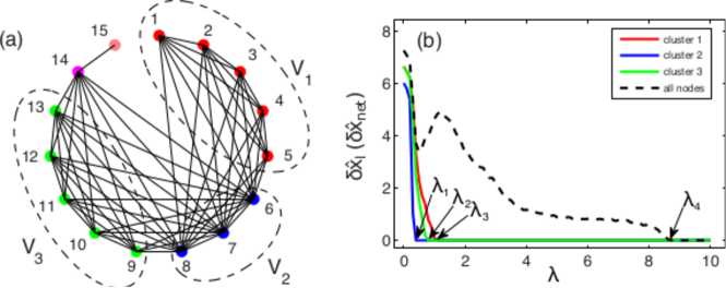
Reference [282] also relates network’s symmetries with the emergence of cluster synchronization states in a Kuramoto model of identical oscillators, when the interactions include a phase frustration preventing full synchronization. In these conditions, the system organizes into a regime of remote synchronization where pairs of nodes with the same network symmetry are fully synchronized, despite their distance on the graph. An application to brain networks suggests that anatomical symmetry may play a role in neural synchronization by determining correlated functional modules across distant locations.
In the framework of networks of communities [283] and networks of networks [249], there are several works seeking for the synchronization performance as a function of the competition between individual communities and the whole network [284, 285, 286]. In particular, Ref. [286] discusses how the degree of the nodes through which two networks are connected influences the ability of the whole system to synchronize. It is shown that connecting the high-degree (low-degree) nodes of each network turns out to be the most (least) effective strategy to achieve synchronization, and the existence of the optimal connector link weights for the different interconnection strategies is reported. On the other hand, Ref. [285] reaches similar conclusions, and observes also intermediate states of inter-community connectivity for which there is a balance between segregation (clustered) and integration (global synchronization) dynamics.
To conclude, chimera states have also been reported in complex networks (for an updated compendium of references the reader is addressed to Ref. [232]). In Ref. [287], the Authors considered two globally coupled populations of identical Kuramoto oscillators with inter-population links randomly switched on or off, resulting in the appearance of stable, breathing, and alternating chimera states. Reference [288] investigated non-locally coupled identical phase oscillators in SF and ER networks, where a coupling function dependence on the shortest length between oscillators is introduced (, with being the global coupling strength and the strength of the non-local coupling). With these settings, chimera states spontaneously emerge out of arbitrary initial conditions for both types of complex networks and oscillators. These states tend to include nodes with high degrees on SF networks, while there is no preference for degree for oscillators on ER ones (see Fig. 23).
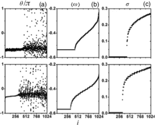
3.4.2 Non-identical systems
In real systems, populations of interacting oscillators are neither homogeneous nor regular in frequencies, and we already saw that a widely studied paradigm is the Kuramoto model, described in Subsection 3.3.4. The first attempt to investigate the role of non-regular topologies was performed in Ref. [289]. It was shown there that introducing some variability in a lattice (by randomly rewiring a few local interactions to long-range connections) leads to a more rapid and robust phase locking than nearest-neighbor couplings, or locally dense connection patterns. When the Kuramoto model is considered on top of a complex network of interactions, Eq. (13) translates to
| (24) |
where is again a global coupling parameter, and is a matrix defining the oscillators’ interactions (a complete graph is recovered by setting for all pairs).
There are two important issues to be discussed about the extension of Kuramoto model to complex networks: the re-scaling factor in the coupling term of the dynamics, and the issue of properly defining an order parameter. In Refs. [290, 247] the implications of different normalizations used in the literature are investigated. One of the most used prescriptions consists in taking , which however has the problem that (in the thermodynamic limit) the coupling term vanishes for all nodes except for those whose degree scales as . Another prescription, used to solve the paradox of heterogeneity (discussed in the previous Subsection), consists in taking . In particular, Ref. [290] considers , being the largest degree in the network, this way decoupling the heterogeneity of the network and the interaction dynamics and, at the same time, having a non diverging limit for . As for the definition of the order parameter, it is worth noticing that the asymptotic magnitude defined in Eq. (14) allows for a complete graph the measurement of the average performance of synchronization. Tailoring for non-complete graphs is the object of many studies, as e.g. those realized by Ichinomiya [291], Restrepo et al. [292], or by Sonnenschein and Schimansky-Geier [293] in the context of complex networks of noisy oscillators.
Early works investigating synchronization in Eq. (24) are those by Watts and Strogatz [245] and Hong et al. [294] for SW networks, and by Ichinomiya [291] and Moreno and Pacheco [295] for SF networks. In particular, Ref. [294] showed (by means of extensive calculations) that any finite probability of rewiring in the Watts-Strogatz model [245] gives rise to a finite critical coupling , and that the scaling is indeed compatible with the mean-field of the globally connected graph. Moreover, diverges as , and the time needed to achieve the coherent state decreases with . In the presence of large degree fluctuations, Ichinomiya proposed to rescale as follows
| (25) |
and found that the critical coupling for uncorrelated random networks with arbitrary degree distribution is
| (26) |
where is the critical point for Eq. (22). When the degree fluctuations are bounded, both and are finite in the thermodynamic limit. However, for power-law degree distributions , the critical coupling vanishes when . A refinement of the latter result has been provided by Restrepo et al. [292], who generalized the mean-field approach, and showed that the coupling strength at which the transition takes place is determined by the largest eigenvalue of the adjacency matrix (). As for the role of the hubs in the synchronization process on top of a SF network, Ref. [295] showed that the relaxation time for the hubs is shorter than that of the less connected nodes, scaling as . Hence, the more connected a node is, the more stable it is.
The mean-field approach allows also to compute the scaling of [296]. For finite , one has
| (27) |
where . For SF networks with , the exponent takes the value if , and for .
Finally, we briefly review clustering and modular synchronization in networks of oscillators [292, 297, 298, 284, 299, 300, 301]. Since the route to complete synchronization is made up of groups of synchronized oscillators that grow and coalesce, structural properties at the meso-scale of the network can be detected by a fine tuning of the coupling strength. In particular, Ref. [302] compared the synchronization patterns in ER and SF networks and showed that even in the incoherent solution, the system self-organizes following different paths: while in SF networks the giant component of the synchronized pairs is gradually increasing with the coupling strength around the largest degree nodes, in ER networks the coalescence of many small clusters leads to a giant component whose size is of order of the system size once the incoherent state destabilizes. Oh et al. [297] studied the Kuramoto model on two different types of modular networks, finding that the synchronization transition crucially depends on the type of inter-modular connections. McGraw and Menzinger [298] found that the promotion of dynamical clusters oscillating at different frequencies hinders in general synchronization.
In Li et al. [300], the interfaces between synchronized clusters emerging due to frustration are explored. An algorithm is there provided able to detect the frustrated nodes located at the overlapping structures of real-world networks. The algorithm was then used to unveil protein functions in a protein-protein interaction network in Ref. [303]. Further, an easily computable measure was introduced in Ref. [301] which locates the effective crossover between segregation and integration in modular networks.
Relay (or remote) synchronization of pairs of nodes that are not directly connected via a physical link (nor via any sequence of synchronized nodes) has been observed in star like motifs [304], and in arbitrary networks through the action of mismatched units [305, 306, 307].
New forms of synchronous solutions have also been found in multi-layer networks [308, 249]. In this latter context, several scenarios have been described: intra-layer synchronization, i.e. a state in which the nodes of a layer are synchronized between them without being necessarily synchronized with those of the other layer [309]; inter-layer synchronization, which, on the contrary, refers to a state where all nodes of a layer are synchronous with their replicas in the other layer regardless of whether or not nodes in each layer are synchronized with the other members of the layer [310, 311]; breathing synchronization (a regime resulting from the competition between an instantaneous intra-layer and a delayed inter-layer coupling [312]), where, depending on the couplings and delay, two frequency groups of oscillators emerge within the same layer, each one synchronized with its mirror in a breathing mode.
Most of the works dedicated to the study of the interplay between network topology and coupled dynamics have been performed considering dynamical models of pure phase oscillators and diffusive couplings. However, many biological systems interact in a rather episodic, or pulse-like, way and the amplitude dynamics of the oscillators are usually not constant, as it occurs in coupled neuronal networks. Lago-Fernández et al. [313] compared the synchronization patterns exhibited by networks of nonidentical Hodgkin-Huxley neurons coupled through pulses and different connectivity topologies. It is found that regular topologies produce coherent oscillations with long transients and slow response times, while completely random topologies give rise to a fast but not coherent response to external stimuli, and SW configurations sustain both coherent global oscillations with a fast response.
In a posterior work, it was shown that different types of neural excitability (different amplitude dynamics) endow neural assemblies with very different dynamical properties [314]. Recently, Ref. [307] compared the behavior of networks with dynamical units having both amplitude and phase dynamics and that of networks of pure phase oscillators. The comparison highlights that synchronization is enhanced when the dynamics of the units is close to a Hopf bifurcation, and that the emerging behavior crucially depends on the topology and on the node frequency distribution [314, 307].
Synchronization phenomena have been used as a useful (and easy to compute) topology probing tool. Several works focused on how synchronization can unveil structural details of the underlying network where the dynamics is developing [315, 316, 317]. It turns out that, in the transient of a synchronization process, topological hierarchies are related to different time scales [315]. On the other hand, based on cluster de-synchronization, Ref. [316] was able to fully detect the modular structure of a network by dynamically changing the weights of the graph’s links. Furthermore, when considering negative interactions (a fraction of which has been shown to be beneficial in Ref. [318]) synchronization in signed networks can be used to unveil the organization of an ecological system, and to analyze the role of each species [317].
Finally, several works dealt with synchronization in networks in which structural and dynamical features coevolve [319, 320, 321, 322, 323, 324, 325]. By introducing different mechanisms for governing the co-evolution (as, for instance, the competition between the reinforcement of those interactions between pairwise synchronized units [319] and the conservation of the total input strength received by each unit [322, 323]), the adaptive network evolves to a state characterized by local synchronization patterns together with an underlying network structure featuring SF and/or modular structures.
4 Explosive synchronization
4.1 Earlier studies on discontinuous transitions in the Kuramoto model
We start this Chapter with a journey on several early studies aimed at showing the possibility of discontinuous transitions in the Kuramoto model of Eq. (13). The main ideas and conclusions of these studies, indeed, have stimulated the recent advancements on explosive synchronization in networked systems, which will then be reviewed in Sections 4.2, 4.3 and 4.5.
4.1.1 The importance of the frequency distribution
In 1984, Kuramoto proved that there are always two branches of solutions in the thermodynamic limit of Eq. (13) [23]. The first one is the trivial solution (corresponding to incoherence), and the second one bifurcates continuously at , with , being the distribution of natural frequencies, characterized by . Kuramoto also found the first evidence of an abrupt synchronization [23]: close to , there is a small-bifurcating solution [238]
which is supercritical for (i.e., when there is maximum at ) and subcritical if (i.e., when is a local minimum).
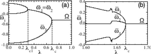
The behavior of Eq. (13) with a discrete frequency distribution was then studied using a Lyapunov function formalism [327]. Precisely, the Lyapunov function was proposed (with being the average frequency) and interpreted as a Hamiltonian of a XY ferromagnet of strength in a random field. The approach allowed to prove that the order parameter is always , and therefore a continuous transition from the phase locked to the incoherent state is impossible. Later on, Ref. [328] proved that the appearance of a macroscopic cluster of mutually phase-locked oscillators takes place continuously when the bifurcation is supercritical, and discontinuously (with hysteresis and bistability) otherwise.
Reference [326] studied how the Kuramoto model de-synchronizes. A transition called frequency-splitting bifurcation is observed: when the coupling strength decreases below only one of the phases splits off from the others, but if the natural frequencies are evenly distributed in an interval, the synchronized state splits into several clusters (see Fig. 24, where the effect is shown for three oscillators). The conclusion is that, although a discrete frequency distribution produces a discontinuous transition in the thermodynamic limit, the transition at any finite size depends on how the natural frequencies are chosen.
Following the same concepts and ideas, Pazó focused on understanding the finite-size behavior of the Kuramoto model [14]. Ref. [14] proved (analytically and numerically) that several frequency distributions (with support on a finite interval) lead to a discontinuous phase transition. First, the Kuramoto model is analyzed in the limit for a uniform frequency distribution , and the critical coupling is deduced for which the order parameter undergoes an abrupt transition from zero to (associated with the emergence of meta-stable states [329]). Then, the finite size effects are studied with natural frequencies that are evenly distributed in the interval . With such a choice of frequencies, Ref. [14] derives a self-consistent equation for a finite population of oscillators that accurately reproduces the numerical results.
Reference [330] further studied the case of a unimodal frequency distribution (depicted in Fig. 25(a)) with a plateau in the interval and symmetric tails behaving as , where is a constant, is a parameter and is the unit step Heaviside function. Figure 25(b) shows that a critical coupling value exists where the system undergoes a discontinuous transition. The order parameter jumps from to . The transition is discontinuous for any value of , as long as the plateau is a finite flat region (i.e., ), and only when the transition becomes continuous.
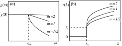
The latter result was extended to asymmetric frequency distributions in 2008 [331]. Going beyond earlier studies on the impact of asymmetries in the frequency distributions [332, 333], Ref. [331] found that a necessary condition for a transition to be discontinuous is to have a flat interval in the region of the frequency distribution where the synchronization seed is generated.
Originally, when Kuramoto considered the subcritical case, was assumed to be a symmetric function around the local minimum at , featuring two local maxima at . The existence of the two local maxima implies that the incoherence solution, , cannot persist up to even as a meta-stable state. Therefore, the lower critical value for the onset of nucleation around is . As is increased, the two clusters grow independently of each other, like two giant oscillators, until for some large coupling value they eventually synchronize. An exact description of the thermodynamic limit of Eq. (13) with a bimodal frequency distribution was found in 2009 [243] for , being the center frequencies of two Lorentzians, and the half width at half maximum, which must verify . Together with the well-known incoherent and partially synchronized states, a third state (consisting of two symmetric clusters of synchronized oscillators near the distribution’s maxima) is found, which later on was termed as the standing wave state [334]. However, the bifurcation sequence suggested by Kuramoto (incoherence standing wave partial synchronization, as sketched in the upper part of Fig. 26)) is not the unique possibility. Actually, such a sequence occurs when the two maxima in the frequency distribution are sufficiently far apart. Furthermore, the conjectured formula for is incorrect in general, being only valid asymptotically in the limit of widely separated peaks. When the frequency distribution is barely bimodal, instead, the bifurcation sequence does not include the standing wave state, and there is hysteresis in the transition. In the intermediate regime, where the peaks of are neither too far apart nor too close, the forward bifurcation occurs via the sequence predicted by Kuramoto, while the backward bifurcation skips the standing wave state and results directly from partial synchronization to incoherence.
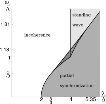
These results were complemented by Pazó & Montbrió [335] with a study in which the minimum and the distance between maxima can be independently modified. In particular, a normalized distribution is considered of the form and similar bifurcation sequences are obtained. The case is of special interest (as there the value at the minimum is always , independently of how close the two maxima are), and results in a sequence incoherence standing wave partial synchronization without hysteresis (even for extremely close to zero).
4.1.2 Effects of noise
The study on noise affects on top of the Kuramoto model started with Ref. [336], where an independent white noise stochastic source was added to Eq. (13), with and ( being the noise intensity and angular brackets denoting ensemble average over independent noise realizations). Assuming a Gaussian frequency distribution, Ref. [336] found that noise makes the critical coupling strength larger but does not change the continuous nature of the transition.
Despite seeming an obvious fact, it is actually hard to prove that the solution is stable for and unstable for . Reference [337] revealed that the incoherent solution is unstable for , but neutrally stable for . Surprisingly, when the problem is studied for small noise, and then the limit is considered of noise intensities going to zero, the results are completely different: the relaxation of to its steady state follows an exponential law for , whereas for the decay rate depends on the frequency distribution [338]. If has a compact support, tends to zero slower than an exponential, but if is supported on the reals, is known only in some cases.
Back in 1991, Okuda & Kuramoto [339] considered the case of Gaussian white noise and a discrete frequency distribution consisting of two equiprobable frequencies . A critical value of the noise intensity is found, below which the system synchronizes either partially (only oscillators with the same frequency synchronize) or globally. Consequently, the bifurcation diagram, shown in Fig. 27(a), has three regimes: asynchronous (referred to as steady), partially synchronized (referred to as independent), and globally synchronized, which overlap in the region QRS depicted in Fig. 27(b), indicating that the transition to synchrony occurs through a region with bistability.
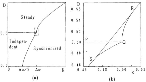
Therefore, with or without noise, the Kuramoto model presents a rather complex behavior as soon as the frequency distribution has two peaks. The case of two peaks equidistant to zero was studied in Ref. [340]. If the maxima are close, , the transition to the synchronous state is continuous. When , the transition is discontinuous with hysteresis. Finally, when the peaks are separated enough, , the transition is also discontinuous with hysteresis, but now the stable synchronized state is characterized by having a time-periodic order-parameter. The case of a more general frequency distribution (which consists in two Lorentzians centered at with the same width parameter ) was studied in Ref. [334]. A critical value for the separation between the maxima, is found, that determines the behavior of the system. For , the bifurcation is supercritical to a stable synchronized state. For , there is a subcritical bifurcation to a synchronized state with no prior onset of synchronization in the peaks of the distribution. And for , there is a transition to a state consisting of two symmetric clusters of synchronized oscillators, called standing waves. As the peaks move far apart (i.e., ), the oscillators in the peaks indeed synchronize, but as , they synchronize at frequencies that are substantially shifted away from the peaks of the native distribution. Actually, Fig. 28, where these results are schematically shown, is remarkably similar to Fig. 26, but the effect of the noise added is to increase the width of each Lorentzian in , having an effective width .
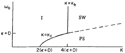
The asymmetric case was studied in Ref. [341] which considered the bimodal distribution . Here, entails essentially different features with respect to the symmetric case (). By comparing Fig. 29 (which shows the stability boundaries for and ) with Fig. 28, one can appreciate how the asymmetry of the frequency distribution changes the stability boundaries: both the region of incoherence and standing waves becomes smaller, whereas the partially synchronized area grows. Finally, Ref. [342] considered a discrete version of the Kuramoto model to explore the transition to synchronization in a population of weakly coupled oscillators. When the coupling strength exceeds some noise-dependent threshold, the population develops spike-like solutions with noisy boundary layers, and its behavior is similar to that of the continuum limit. However, a much more complicated behavior occurs for sub-threshold coupling strengths, where the finite population displays complicated temporal dynamics (ephemeral coherent structures, switching patterns).
4.1.3 Generalizations of the coupling pattern
Another streamline of research analyzed the effects of changing the original (uniform, all-to-all) connectivity of Eq. (13). Reference [343], for instance, generalized the Kuramoto model to account for intersegmental coordination of neural networks, responsible for generating locomotion in the isolated spinal cord of lamprey. Reference [343] considered that each oscillator only has two nearest neighbors, and assumed that all upward and downward coupling strengths are equal. Not only most of the experimental observations were reproduced, but also stable phase locked motions (corresponding to traveling waves) as well as drifting motions were found.
A more general approach was followed in Ref. [344], which assumed a Gaussian and an underlying topology of a -dimensional hypercubic lattice. Namely, is taken only if and are nearest neighbors in the lattice. The -lattices self-organize in clusters of entrained oscillators, for which the lattice dimension determines if some of them develop into a macroscopic size.
Reference [345] revisited the problem with the aim to give more accurate predictions by means of a real-space renormalization-group analysis. Reference [345] considered the case of a generic coupling pattern satisfying (therefore the Kuramoto model is encompassed as the case ). Reference [345] first showed that the global behavior of the lattice strongly depends on the frequency distribution. If the variance of is not defined, its asymptotic behavior can be written as , with , while if a frequency distribution has finite variance, it can be studied by taking . Assuming that the whole -dimensional lattice is divided into a set of hypercubes with an equal linear scale , Ref. [345] demonstrated that synchronization only arises in a -lattice when . In particular, this implies that synchronization is impossible in any -lattice if (e.g., for a Lorentzian), while it is possible for any frequency distribution with finite variance (e.g., for a Gaussian) if the lattice has .
Later on, however, Ref. [346] found that global synchronization is actually impossible for all -lattice. Precisely, given a Gaussian frequency distribution, and oscillators in a -lattice coupled with strength , the probability of phase-locking is found to verify , for all finite and . Furthermore, dropping the assumption of a Gaussian distribution and assuming only that has finite mean and finite non-zero variance, the former result remains valid. Therefore, there is no critical dimension for phase-locking, because the probability tends to zero exponentially fast for any -lattice.
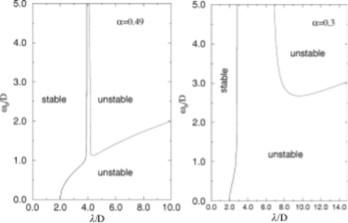
Reference [347] proposed one of the first models in which the interactions among the oscillators are random. In order to have an analytically tractable model, it is considered that the interaction between oscillators and (which are placed on a lattice) is , where is a control parameter, is the number of interacting neighbors of each oscillator, and are random parameters taken from a distribution . For the particular case (being a parameter and the Dirac function), the order parameter comes out to be proportional to the original Kuramoto parameter , , thus randomness causes a decrease in the order parameter. The symmetric case (i.e., ) results in a disordered system even for , which was called a spurious glass-like phase. Reference [348] proposed another model in which the interaction is assumed to be an independent random variable with normal probability distribution, (where is the control parameter). Numerical evidence is obtained of a new type of ordered phase that is analogous to those observed in a variety of glassy systems.
Reference [349] studied the case in which the underlying network topology is a tree with branching ratio , being the oscillators at the leaves, under the hypotheses that the coupling strengths vary with the distance and are distributed over a hierarchy of values. Specifically, it was assumed that intra-cluster interactions are weaker than inter-cluster ones. It is shown that distinct regimes are emerging depending on whether the branching ratio is smaller or larger than the critical value .
Reference [350] provided a stability analysis of the Kuramoto model in terms of appropriate Lyapunov functions, recovering all the previous results for fully connected graphs, and obtaining new ones for generic topologies. Finally, Filatrella et al. [131] proposed a modification of the Kuramoto model to account for the effective change in the coupling constant suggested by some experiments on Josephson junctions [351, 352], laser arrays, and mechanical systems. Namely, Ref. [131] proposed a variation of the Kuramoto model that accounts for change of the coupling with the number of active oscillators: the natural frequencies are taken from a Lorentzian with zero average and width, and the coupling is taken to be , where the parameter is a heuristic measure of the strength of the feedback mechanism. The resulting model is analytically tractable, and predicts that both first and second order phase transitions are possible, depending upon the value of the parameter that tunes the coupling among the oscillators. For the evolution from the incoherent value to the partially coherent state is continuous (see Fig. 30(a)). When , the critical value where the transition to synchrony occurs changes for the forward and backward transitions, yielding hysteresis, whose width is larger for the larger (as it is evident by comparing the case in Fig. 30(b) to the case in Fig. 30(c)).

4.2 Explosive synchronization in complex networks
Unfortunately, the scientific community was initially somehow apathetic to the many results summarized in the previous Section, and such a situation (of almost indifference) persisted lamentably for longtime, up to when the scientific community started to be interested in the study of the transition to synchrony in complex networks.
4.2.1 Explosive synchronization in networks of frequency-degree correlated oscillators
In Ref. [15], an unweighted and undirected network of Kuramoto oscillators [187] is considered, whose equations of motion are
| (28) |
where stands for the natural frequency of oscillator , is the coupling strength, and are the elements of the network’s adjacency matrix.
Reference [15] actually introduced a specific (ad-hoc) form of correlation between the natural frequencies and the degrees of the oscillators. Namely, the natural frequency of node was imposed to be proportional to its degree (). Once such a correlation is artificially imposed, different networks (generated by the algorithm of Ref. [353]) are studied, having the same average connectivity but variable heterogeneity properties (i.e. ranging from ER to Barabási-Albert (BA) graphs, depending on the value of a single parameter ).
The results are summarized in Fig. 31. The synchronization diagrams for several values of are plotted as a function of the coupling , for both forward and backward transitions. The transition is soft and reversible for most values of , but when (corresponding to a BA network) an abrupt behavior appears, with the parameter remaining close to zero up to a point at which it suddenly jumps to . As the critical coupling is different for the forward and the backward diagrams, the transition is irreversible and displays a hysteresis loop.
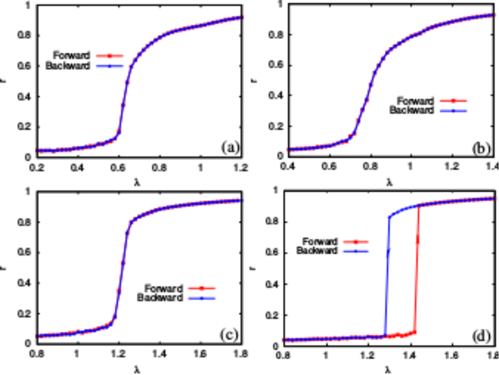
Reference [15] offers also an analytical study of a specific star configuration, composed of a central node (the hub ) and peripheral nodes (the leaf nodes), each one labeled by the index (). By setting the frequencies of the central node (), and that of the leaves ( ), the equations of motion can be written as
| (29) |
Then, using the average phase of the system (, where is the average frequency) as a rotating frame, the equation for the hub evolution can be rewritten as
| (30) |
The condition for stability of the hub locking solution () allows one to obtain the backward critical coupling value as , and the order parameter at the critical point is found to be , that is at the critical point, confirming the existence of a discontinuity in the transition.
The same degree-frequency correlated star of Eqs. (29) was studied in Ref. [20], where the origin of the hysteresis loop was rooted in the properties of the basin of attraction of the synchronization manifold. Ref. [20] rewrote Eq. (29) as , where , and . Then, the locking manifold can be defined as , where is a constant. The condition yields the minimal coupling that enables the existence of : , which corresponds to the backward transition.
To obtain insight on the forward transition, Ref. [20] provided numerical evidences that (for ) the local attractiveness of becomes global, i.e. any state (even incoherent) is attracted to for coupling strengths above . This fact (together with the theory developed in Ref. [354]) can be used to reformulate the phase locking problem between the hub and leaves as a perturbation of an identical synchronization problem. In such a latter framework, the condition for coherence gives
| (31) |
where is a constant which depends on the chosen initial conditions. In Fig. 32(a) it is shown how numerical simulations are in excellent agreement with the predictions of Eq. (31).
The results can be extended to the case of SF networks with small mean degrees, that can be considered, indeed, as a collection of stars of different sizes. For , , but . In a SF network with degree distribution the expected degree of the largest hub scales as . Therefore, the expected scales as
| (32) |
As it can be seen in Fig. 32(b) the approximation gives a very good fit for SF networks with .
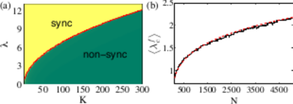
The problem of calculating the forward critical point in a frequency-degree correlated star has been very recently reconsidered by several groups, which applied dimensional reduction techniques [355] and the Ott-Antonsen method [241]. The first approach was applied independently by Vlasov et al. [356] and Xu et al. [357]. Taking , the Eq. (29) can be reduced to
| (33) |
where is the frequency difference between the hub and leaf node. By defining , Eq. (33) is rewritten as
| (34) |
where , and . The Watanabe-Strogatz approach can be used in systems of identical oscillators driven by a common force (having the general form ), as it is the present case. The phase dynamics of the nodes can be constructed by constants as
| (35) |
where and are global variables, and are constants depending on the initial condition of the systems. In the thermodynamic limit () such a transformation allows to separate the evolution of the and variables, and gives . Therefore, the equation of the order parameter can be written as [356, 357]
| (36) |
which describes the collective dynamics of system (29) in terms of the ensemble order parameter, and can be used even for small values of in case of random initial distributions. In the phase space of the ensemble order parameter, the synchronous state corresponds to a fixed point (with ) and a fixed phase . All the other solutions of Eq. (36) represent various incoherent states. If Eq. (36) is rewritten in its Cartesian coordinates , the null-clines of the system can be studied as a function of the coupling , allowing the calculation of the forward critical coupling [356, 357]
| (37) |
It can be seen that the approximation (31) is a good estimation of the latter result for large , where .
A similar dimensional reduction has been provided in Ref. [358], in which an extension of the model is presented where random perturbations affect the frequencies of leaves. The results show that for small perturbations the synchronization phase transition is still discontinuous, while for large perturbations the transition becomes continuous.
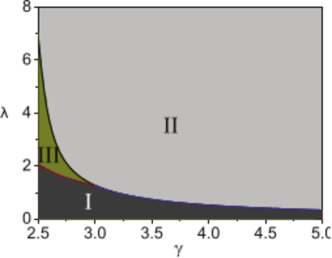
In Ref. [359] the case of a star graph with arbitrary natural frequency is studied. Then, the systems’ equations become
| (38) |
The transition to synchrony of this system is discontinuous when , where is a certain critical frequency difference.
Beyond a star graph, analytic results for general networks (under the assumption that ) were given by Peron et al. [360]. In the continuous limit, the equation of the system is
| (39) |
Ref. [360] shows that (in such a limit) the forward critical coupling is .
Notice that this critical coupling differs from the usual value for symmetric .
Even though the calculations in Ref. [360] identify the frequency and degree distributions, they do not account for degree-frequency correlations, and therefore fail in predicting if the transition is explosive or continuous. The issue was addressed in Ref. [359], where the annealed network approximation was used to solve Eq. (28) under the assumption . An implicit solution for the order parameter
| (40) | |||||
| (41) |
is found. Following such a solution, ER networks always undergo second order transitions, whereas the nature of the transition in SF networks depends on the heterogeneity parameter , as shown in Fig. 33: a first-order-like transition is found for , but a second-order transition occurs for . A hybrid phase transition is found for , combining a jump of the order parameter and critical phenomena at the critical point. This is actually a first indication that not all SF networks are able to sustain explosive synchronization (ES), even when they are fully frequency-degree correlated, a subject that will be reconsidered afterwards [22].
In a number of works, various generalizations of the frequency-degree correlation have been analyzed. In Ref. [361], a more general joint distribution is considered. The phase-locking behavior of the system is examined, and it is found that the criterion for locking is , being the order parameter. From this expression one can deduce that the nodes with low degree are the last ones to get phase-locked for sub-linear correlation (), whereas super-linear correlation () induce the last drifting nodes to be the hubs. These two qualitatively different behaviors are separated by the critical case of linear correlations () for which disappears, and the oscillators lock simultaneously.

In Ref. [363], instead, the possibility of a partial frequency-degree correlation is considered, and it is shown that a small fraction of correlated nodes is enough to obtain ES in a SF network. The issue of partial correlation has been dealt with also in Ref. [362], where only vertices with degree larger than a certain threshold are supposed to exhibit the degree-frequency correlation, whereas the other vertices have random natural frequencies with distribution . This latter feature can be formally enunciated through a joint probability distribution (for a node of degree and natural frequency ) given by , where and are, respectively, the Dirac delta and the Heaviside step functions, and is the degree distribution. A mean-field calculation shows that the correlation of the highest degree nodes is enough to promote ES in BA networks. The results are shown in Fig. 34: by imposing a partial degree-frequency correlation not only it is possible to keep ES in the cases where it already happens with full correlation (Fig. 34(b)-(c)) but, unexpectedly, ES emerges also in cases in which full correlation would have prevented it (Fig. 34(a)).
Other works have tested how ES is affected by modifications to the original Kuramoto model. In Ref. [101] it is reported that ES persists (and is even enhanced) in modular BA, correlated networks. In Refs. [364], the model of Ref. [15] is modified to include delay times phase shifts [357], and it is found that an appropriated choice of parameters can enhance or suppress ES. An example of the effect of time delay is shown in Fig. 35.
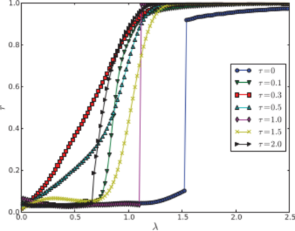
Reference [365] generalized the relationship as , where is a normalization to avoid homogenization of the frequencies when is small, and is in the range , thus including the possibility that and are anti-correlated. For positively k- correlated networks () ES remains unmodified for up to , but it transforms to a second-order transition for any value. The effect of degree mixing in the model is also considered, and it is pointed out that assortativity has a strongly destructive effect on ES. In Ref. [366] a frequency-degree correlated BA network is rewired to introduce assortativity, and it is pointed out that a moderate disassortativity favors the ES, which instead is destroyed for assortative mixing.
A detailed study of the role of the assortativity in ES is provided in Ref. [22]. With the aim of inspecting whether or not ES depends on the chosen network model, Ref. [22] comparatively considers ensembles of networks obtained with the BA algorithm and networks displaying the same SF distributions, but constructed by the so called configuration model (CM, [367]). For both networks, parameters were assumed to be and , and the oscillators’ frequencies were distributed so as to determine a direct correlation with the node degree ().
The results reported in Fig. 36 show a dramatic dependence of the ES behavior on the underlying SF network model used, despite displaying the same . The forward and backward continuations of the order parameter are totally different for BA (Fig. 36(a)) and CM (Fig. 36(b)) networks, and indicate that a crucial condition to obtain irreversibility is having an underlying growing process through which the SF topology is shaped.
One customary way to quantify the amount of degree correlation with a single parameter is using the Pearson correlation coefficient , which can be calculated as [368]:
| (42) |
where and are the degrees of the nodes at the ends of the th link, with . Actually, one has that , with positive (negative) values of quantifying the level of assortative (disassortative) mixing. The BA model does not exhibit any form of mixing in the thermodynamic limit ( as as ), while a random CM produces highly disassortative networks.
Finally, Ref. [22] studies the impact of increasing/decreasing the assortativity mixing on a network with a given degree sequence taken from a power law distribution . SF networks with given and tunable levels of degree mixing can be generated by the rewiring algorithm of Xulvi-Brunet and Sokolov [369]. Two ensembles of BA and CM networks are then constructed, all of them having the same degree distribution, but different values of the assortativity coefficient . Figures 36(c)-(d) illustrate the effect of degree mixing on ES. Extensive numerical simulations were performed at various values of , for slopes ranging from to , and for the same mean degree . The most relevant result is that, regardless of the specific SF network model, the hysteresis of the phase transition is highly enhanced (weakened) for positive (negative) values of , and that there is an optimal (positive) value of where the irreversibility of the phase transition is maximum. The enhancement is far more pronounced in BA (Fig. 36(c)) than in CM (Fig. 36(d)) networks.
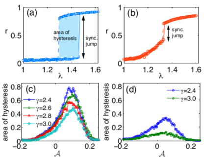
4.2.2 Explosive synchronization in frequency-disassortative networks.
While earlier works concentrated on ad-hoc imposed correlations between the node degree and the corresponding oscillator’s natural frequency, posterior studies highlighted that a sharp and discontinuous phase transition is by no means restricted to such rather limited cases, but it constitutes, instead, a generic feature in synchronization of networked oscillators. Precisely, Ref. [17] gave a condition for the transition from unsynchronized to synchronized states to be abrupt, and demonstrates how such a condition is easy to attain in many circumstances, and for a wide class of frequency distributions.
The basic idea, which evokes the Achlioptas process [9] described in Section 2.2, is avoiding that oscillators behave as cores of a clustering process, where neighboring units begin to aggregate smoothly and progressively. As the synchronization seeds are the aggregations of nodes with close frequencies, the procedure introduces then a frequency disassortativity in the networks. The practical realization of such a condition is made by imposing explicit constrains in the frequency difference between each node and the whole set of oscillators belonging to its neighborhood [17]:
| (43) |
In practice, a threshold for the frequency gap is set, and the network is then grown by means of a conditional CM approach: after having initially distributed the oscillator’s frequency from a given frequency distribution, pairs of unconnected nodes are randomly selected, and a connection between the nodes is established only if they verify the condition (43). The process is repeated until the network acquire a given, desired, mean degree , and the resulting adjacency matrix is used to simulate the Kuramoto model (28).
Figure 37 reports the results obtained by setting as a uniform frequency distribution in the interval . Panels (a) and (b) show the phase synchronization index as a function of the coupling strength. In particular, Fig. 37(a) (resp. (b)) illustrates the case of a fixed mean degree (of a fixed frequency gap ), and reports the results for the forward and backward simulations at different values of (). A first important result is the evident first-order character acquired, in all cases, by the transitions for sufficiently high values of .
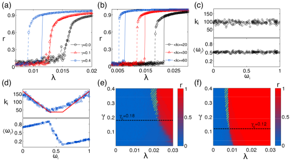
A second relevant result of Ref. [17] is the spontaneous emergence of degree-frequency correlation features associated to the passage from a second- to a first-order like phase transition. While such a correlation was imposed ad hoc in Refs. [15, 16], here the condition (43) creates for each oscillator a frequency barrier around , where links are forbidden. The final degree will be then proportional to the total probability for that oscillator to receive connections from other oscillators in the network, and therefore to . This is shown in (c) and (d) of Fig. 37, where the degree that each node achieves after the network construction is completed is reported as a function of its natural frequency , for . Precisely, the upper plot of Fig. 37(c) refers to the case in which no degree-frequency correlation is present. In the upper plot of Fig. 37(d), instead, it is reported the case (a value for which a first-order phase transition occurs) and the (conveniently normalized) function , with for , and elsewhere, which gives evidence of the emergence of a very pronounced V-shape relationship between the frequency and the degree of the network’s nodes. The latter fact marks a noticeable difference between the approach of Ref. [17] and those described in the previous Section. Here, indeed, a pattern of frequency-degree correlation emerges spontaneously, and is not artificially imposed. Moreover, the emerging pattern i) is clearly non-linear; ii) it depends explicitly on the frequency distribution ; iii) it is in general V-shaped.
Finally, Fig. 37(e) and (f) report in the space, for and , and show that the rise of a first-order like phase transition is, indeed, a generic feature in the parameter space. The horizontal dashed lines in panels (e) and (f) mark the values of , separating the two regions where a second-order transition (below the line) and a first-order transition (above the line) occurs. The fulfillment of Eq. (43) leads to an explosive transition for a very wide class of distributions of the oscillators’ natural frequencies, as shown in Fig. 38(a)-(b) for a Rayleigh distribution.
Furthermore, Ref. [17] discusses also several ways of even softening the condition of Eq. (43). For instance, a frequency gap in the network growth can be introduced as , where indicates the average value over the ensemble . The results of this (local mean field) gap in a homogeneous frequency distribution are shown in Fig. 38(c)-(d). It is worth noticing that a strict application of the gap condition for non uniform frequency distributions implies that oscillators at different frequencies would in general have a different number of available neighbors in the network. That’s why a natural extension is to consider a frequency-dependent gap defined by . The gap condition for the construction of the network is now to fix the value of , and accept the pairing of nodes when . The generic case is again that of an explosive transition, with pronounced frequency-degree correlation features, as long as is symmetrical. Panels (e) and (f) of Fig. 38 report the case of a Gaussian distribution limited to the frequency range , centered at , and given by , with .
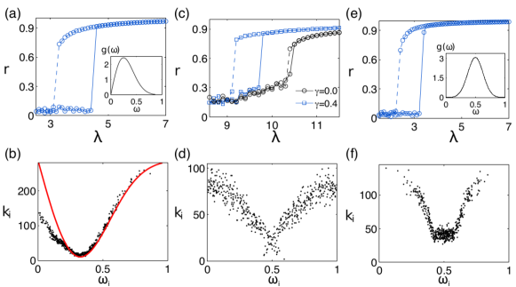
Reference [370] also focused in the idea that ES phenomenon is rooted in preventing oscillators from behaving as the cores of clustering processes. By the use of a constructive gap scheme similar to that of Ref.[17], it is found that frequency disassortativity is accompanied by a strong increase of degree disassortativity. The frequency-equivalent of the Pearson coefficient in Eq. (42) is
| (44) |
where , are now the frequencies of the nodes at the ends of link . From Fig. 39, it can be easily seen that, as the gap parameter increases, both degree- and frequency-assortativity coefficients and stay close to zero up to the critical value , and then become increasingly negative.
The same idea of a gap condition is used in Ref. [371] in a completely different context, i.e. an ensemble of coupled maps:
| (45) |
where is the logistic map, and the parameter is the dimension-less grow factor of element . In Ref. [371], the connectivity on the ensemble is generated by imposing the gap restriction , and ES and hysteresis are observed as a consequence. This latter fact gives a clue on the vast generality of the gap approach, which provides, indeed, a rather good comprehension of the inner mechanisms of ES, and can be extended to a broad variety of systems.
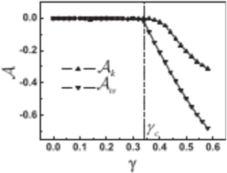
4.2.3 Explosive synchronization in frequency-weighted networks of oscillators
Motivated by the results reviewed in the previous Subsection, Ref. [18] further extended the study to the case of a network with given frequency distribution and architecture, for which the only action that an external operator can perform is a weighting procedure on the already existing links. Namely, Ref. [18] combined the information on the frequency mismatch of the two end oscillators of a link with that of the link betweenness (in the more general case), and demonstrated that such a weighting mechanism has the effect of inducing (or enhancing) ES for both homogeneous and heterogeneous graph topologies, as well as for any (symmetric or asymmetric) frequency distribution.
We follow the path of reasoning of Ref. [18], and start by modifying Eq. (28) as
| (46) |
where
| (47) |
is the weight factor to be applied to the (existing) link between nodes , being the elements of the adjacency matrix that uniquely defines the network, and a constant parameter which possibly modulates the weights. The strength of the node (the sum of all its links weights) is then .
Figure 40(a) reports the results for a ER network of size , and several frequency distributions within the range . For the simplest case of a uniform frequency distribution, the un-weighted network ( in Eq. (46)) displays a smooth, second-order like transition [dark blue curve in Fig. 40(a)], whereas the effect of a linear weighting factor () is that of inducing ES in the system, with an associated hysteresis in the forward (solid line) and backward (dashed line) transitions.
More importantly, such a drastic change in the nature of the transition seems to be independent of the specific frequency distribution , as long as they are defined in the same frequency range . The results are identical for symmetric (homogeneous, Gaussian, bimodal derived from a Gaussian) and for asymmetric (Rayleigh, a Gaussian centered at but with just having the positive half) frequency distributions, indicating the existence of a sort of universal behavior for homogeneous graph’s topologies.

Figure 40(b) shows the existence of a parabolic relationship between the strengths and the natural frequencies of the oscillators (associated with the passage from a smooth to an explosive transition). This relationship has been obtained analytically (see Eq.(54)), and perfectly fits the numerical results. The emergent correlation features shape a bipartite-like network, where low and high frequency oscillators are the ones with maximal overall strength.
Furthermore, the weighting procedure inducing ES appears to be really general, because it applies for a large family of detuning dependent functions. As an example, Fig. 41 describes the case of nonlinear weighting procedures [ in Eq. (46)]. There, and are set, and ER graphs (Fig. 41(a)), together with random networks (where each node has exactly the same number of connections, ) are considered (Fig. 41(b)) (the latter case is obtained by a simple configuration model, imposing a -Dirac degree distribution).
A generic non-linear function of the frequency mismatch is able to induce ES in all topologies, and the effect of a super-linear () weighting (a sub-linear () weighting) is that of enhancing (reducing) the width of the hysteretic region.
When networks are heterogeneous, Ref. [18] suggests to use, as a new weighting function,
| (48) |
with being an extra tuning parameter, and being the edge betweenness associated to the link , defined as the total number of shortest paths (between pairs of nodes in the network) that makes use of that edge. The results are reported in Fig. 42. While the case corresponds to a smooth transition, moderate (positive or negative) values of establish abrupt transitions to synchronization.

In order to rigorously predict the onset (and nature) of the explosive transition, Ref. [18] analytically examines the thermodynamic limit in which oscillators form a fully connected graph: . By assuming the following definitions,
| (49) | |||||
| (50) |
the evolution equations can be expressed in terms of trigonometric functions as . In the thermodynamic limit, the solution (in the co-rotating frame) is
| (51) |
The definition of and implies that
| (52) | |||
When all oscillators are close to synchronization, one can assume that , and therefore , where is the strength of a node with frequency . As a consequence, Eq. (51) takes the form
| (53) |
which is a second order ordinary differential equation, whose integration yields . For instance, given a uniform distribution in the interval , the resulting strength is the second order polynomial
| (54) |
which fits the numerical results of Fig. 40(b). The analysis allows determining the dependence of on as , where . In Ref. [18] it is shown that is indeed a multi-valued function (for values of above a given threshold). Similar results are also reported in Ref. [372], which used a slightly modified weighting function
| (55) |
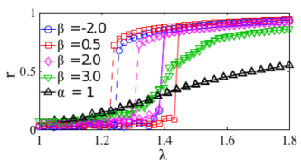
In Ref. [61], Zhang et al. proposed a simpler alternative weighting method:
| (56) |
For symmetric frequency distributions (such as a random, a Lorentzian, or a Gaussian distribution), the model of Eq. (56) induces ES.
The model is, however, less effective in generating ES for asymmetric frequency distributions. In the mean field approximation, Eq. (56) yields . Therefore, one can write
| (57) |
Then, setting as reference frame the one rotating with the average phase of the system, we have , where is the average frequency of the oscillators. For a symmetric , we have . Letting , Eq. (57) becomes
| (58) |
In the phase locking state, , and therefore one has
| (59) |
which implies that two equal clusters form: one including the clockwise, and the other the counterclockwise oscillators. Both values of and gradually approach zero with increasing . This fully confirms the observation in Fig. 43(b). Then, the order parameter takes the form . Substituting Eq. (59) in such a latter expression, one obtains , which is independent on , provided it is symmetric. This result implies that ES exists only for , where has a strong discontinuity from 0.707 to 0.
In the case of asymmetric frequency distributions, a similar calculation gives instead
where , and is the Heaviside step function. In this case, there is a strong dependence on , and Ref. [61] shows that continuous or discontinuous transitions emerge for different frequency distributions.
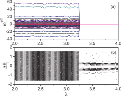
The analytic study of Eq. (56) was tackled by Hu et al. in Ref. [373], where the forward critical coupling was calculated with the use of the method introduced in Ref. [237]. In the limit a density function can be defined, which denotes the fraction of oscillators with frequency whose phases have values between and at time . satisfies the normalization condition for all and . The evolution of is governed by the continuity equation:
| (60) |
Using the expression obtained in Eq. (57), the velocity in the thermodynamical limit can be written as
| (61) |
When the coupling strength is relatively small, all oscillators are rotating in the unit circle according (almost exclusively) to their natural frequencies. This corresponds to an incoherent state . Therefore, the point at which such a state loses its stability can be extracted, providing a prediction for the forward critical point. Specifically, let one consider a small perturbation from the incoherent state, i.e. . Then, the linearized form of the continuity equation (60) is
| (62) |
where
| (63) |
Now can be expanded into a Fourier series as , where stand for higher harmonics. The equation becomes
| (64) |
and can be solved in a self-consistent way. In particular, when is an even function, Eq. (64) becomes
| (65) |
i.e., when changes from negative to positive, the incoherent state loses its stability. For any specific one can then use this condition to determine the critical coupling strength for the forward phase transition. Several examples of this calculation are reported in Table 4 .
| Frequency distribution | Critical equation | |
|---|---|---|
| , 0 otherwise | , | 2.65 |
| , | 4 | |
| , | 2.68 | |
| , | ||
| , |
Xu et al. [374] completed the analysis initiated in Ref. [373], and calculated all possible steady states in the model of Eq. (56), which include the incoherent state and the two-cluster synchronous state already deduced in Ref. [373], but also a traveling and a standing wave state. Reference [374] demonstrated that the incoherent state is only neutrally stable below the synchronization threshold. The amplitude equations near the bifurcation point are derived according to the center-manifold reduction, and non-stationary standing wave states are predicted to exist in the model. Figure 44 reports all possible solutions for a fully connected Kuramoto ensemble with uniform frequency distribution , .
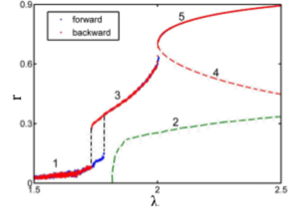
More detailed information on the microscopic mechanisms underlying ES in the model of Eq. (56) can be found in Ref. [19], where a local order parameter, , is introduced
| (66) |
where is a, sufficiently long, time window. is 1 for any two phase-locked oscillators, zero for all pairs of fully uncorrelated oscillators, and will take a value between 0 and 1 for any two partially correlated oscillators. Figure 45 reports the values of for: (a)-(d) fully connected, (e)-(h) ER and (i)-(l) uncorrelated CM networks, for four representative values. Only small synchronized clusters of oscillators exist for , while a giant synchronized cluster shows up suddenly right after , indicating that the small synchronized clusters suddenly merge together right at .
The similarity with the Achlioptas process of EP is even clearer from looking at Fig. 45, where it is seen that, below , links are always generated among those nodes with close frequencies. As a consequence, separated clusters form for up to , where instead (and suddenly) all clusters merge together to mold a giant one. To quantify the analogy with EP, an equivalent suppressing rule is introduced. From Eq. (57), the evolution of the phase difference is given by
| (67) |
When the two oscillators and are phase-locked, one has =0 and therefore
| (68) |
whose maximum value gives a necessary condition for the phase-locking between two oscillators:
| (69) |
Equation (69) can be considered as a suppressive rule for pair wise synchronization: as takes a rather small value when , only those pairs of oscillators with smaller frequency differences can satisfy the condition (69) and thus form synchronized clusters. When all the free oscillators have been attracted to the synchronized clusters, the further increase of cannot make the synchronized clusters become larger, but makes the clusters to merge each other suddenly, this way producing the significant jump on observed in the explosive transition.
Reference [19] shows also that the suppressive rule (69) can actually guide manipulative processes to enhance or quash ES. For instance, one can randomly pick a pair of nodes and then artificially re-adjust the network by exchanging their frequencies if the quantity
| (70) |
decreases (or increases), where stand for the neighborhoods of nodes , resulting in a enhanced (suppressed) ES, as it occurs for the Achlioptas algorithm in EP.
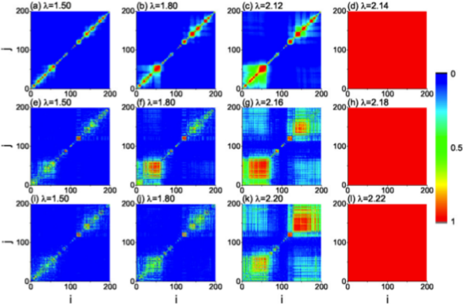
Reference [375] considers the effect of using [in Eq. (56)] frequency distributions not centered in 0, and specifically studies the case of uni-modal frequency distributions (Lorentzian, Gaussian, triangle), displacing their central frequency from to , which is then used as a parameter.
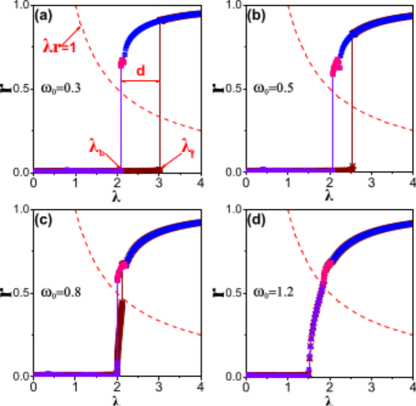
Figure 46 plots the phase diagrams when increasing , and shows that the hysteresis area significantly shrinks, mainly due to the decrease of the forward transition point , while the backward transition point remains unchanged.
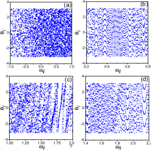
An interesting view on microscopic processes in both the first-order and second-order cases can be obtained from Fig. 47. Here, the incoherent steady state is explored for two values of the central frequency: (Fig. 47(a)-(b), which causes ES), and (Fig. 47(c)-(d), for which the transition is reversible). In all the cases of Fig. 47 the coupling is , i.e. below the synchronization threshold, and therefore . However, essential microscopic differences exist between these incoherent states. While the phases are randomly distributed just below the forward threshold in the ES case (Fig. 47(a)), the incoherent state of the corresponding backward continuation (Fig. 47(b)) is non-trivial, showing the remaining of small clusters with fine structures. In the second order case with , these microscopic structures appear in the incoherent state of both the forward and the backward (Fig. 47(c)-(d)) continuations. Such microscopic differences reveal that, as the frequencies distribution is not symmetric around , formation of micro-clusters occurs, and prevents ES.
This is actually due to the suppression rule of Eq. (69). All the pairs of nodes whose frequencies have different sign fulfill , and therefore, being 0 in the incoherent state, they do not synchronize. An asymmetrical frequency distribution will reduce the number of possible pairs of nodes with frequencies of opposite sign, and therefore an increasing number of pairs will be able to form synchronization seeds, so that eventually ES is destroyed for large enough .
Following the same line of investigation of microscopic mechanisms underlying ES, Ref. [376] proposed the use of an effective topological network whose structure explicitly reflects the interplay between the topology and dynamics of the original system in an individual basis, and therefore, is able to easily identify the nodes which actually act as synchronization seeds. The effective adjacency matrix is given by
| (71) |
where is the frequency detuning, and the maximum possible detuning present in the system in order to guarantee .
In order to quantify the role of each node in the synchronization process, Ref. [376] extracts the most important nodes in the network defined by , i.e. the standard eigenvector centrality measure of , obtaining the effective centrality vector , whose -th component quantifies the potential of node to behave as a seed of synchronization.
Figure 48 reports the comparison between and its topological counterpart , the eigenvector centrality extracted from the original adjacency matrix . For ER networks (Fig. 48(a)), the distribution of the components of the vector as a function of the corresponding node’s natural frequencies shows the existence of many seeds of synchronization with natural frequencies close to . This allows characterizing the connection between the micro-scale and the macro-scale of the network in a much better way than , whose components are instead uniformly distributed. For SF networks (Fig. 48(b)), the synchronization seeds are the hubs, and therefore and provide essentially the same information.
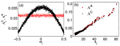
4.2.4 Noise induced explosive synchronization
As discussed in Subsection 4.2.1, a simple (yet artificially engineered) degree-frequency correlation gives explosive synchronization on sufficiently heterogeneous networks [15, 16]. An extension of such artificial process is proposed in Ref. [377], where the frequencies of oscillators are correlated with (but not fully determined by) the local network’s properties, such as the degree. More precisely, the evolution of phase oscillator is taken to be
| (72) |
where , where is a noise term taken from a random homogeneous distribution in the range [, ]. returns the case of Ref. [15]. Reference [377] considers realistic C. elegans neural networks, stretched exponential networks and SF networks with mild heterogeneity (i.e. in the degree distribution ). Given that the synchronized solution is composed of a cluster with uniform angular velocity , the rotating reference frame involving the change of variable is defined as follows
| (73) |
and the local order parameter is defined as
| (74) |
having a magnitude . Substituting Eq. (74) into Eq. (73), one gets
| (75) |
From Eq. (75) it is clear that, if , can reach a steady point expressed by and becomes phase-locked; otherwise the oscillator drifts forever.
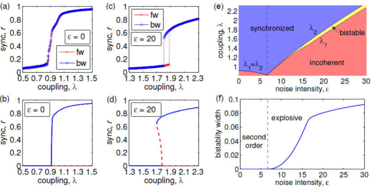
The self-consistency condition for the steady-state order parameter is [377]
| (76) |
which can be used to predict the evolution of synchronization, and where is the so-called joint probability distribution of degree and frequency.
In the absence of noise, the transition from incoherent to synchronized states seems to be second-order like for both real and synthetic networks. The trend can be accurately predicted by the self-consistency condition (76), and is shown in Fig. 49(b). For sufficient large noise, however, ES takes place with a clear bistable region on the less heterogeneous networks (see Fig. 49(d)). If and denote the forward and backwards critical coupling strengths, the width of hysteresis loop is From Figs. 49(e) and (f), one sees that the transition from incoherent to synchronized phases is second-order like until a critical value of the noise (denoted by the dashed lines). Therefore, ES can be promoted by noise mechanisms.
Reference [378] suggested to focus on the angular velocity of oscillator . With Gaussian noise , the dynamics is ruled by
| (77) |
where accounts for an inertia term, denotes the friction constant, and is the order parameter. In particular, Ref. [378] assumed , where is a stochastic noise (like a temperature in units of the Boltzmann constant). Furthermore, a uni-modal is considered, with width . At , the dynamics resembles that of a Brownian mean-field model [379]. In the absence of inertia, reproduces the Kuramoto model [23, 237, 238], while gives the model of Ref. [336].
Figure 50(a) reports the phase diagram in the parameter space. The shaded blue surface is a first-order transition surface. Under (outside) this surface, the synchronization transition is abrupt and explosive (continuous). To furnish a better intuitive illustration, Fig. 50(b) shows the behavior of as a function of noise . For large , the change of is continuous and overlapped between forward and backward transitions. With decreasing , however, ES takes place and the width of hysteresis loop becomes larger.
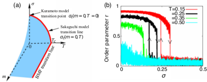
The effect of noise on synchronization was actually observed in other types of synchronization models [380, 381, 382, 383, 384, 385, 386]. For instance, for a positive correlation and sufficient wide frequency distribution, an intermediate noise can lead to the maximal hysteresis loop in the synchronization diagram of FitzHugh-Nagumo oscillators operating on top of SF networks [63].
4.3 Explosive synchronization in generalized Kuramoto models
In the original Kuramoto model (Eq. (13)), the sign of the coupling strength is assumed to be positive, implying that the interactions among oscillators are always attractive. However, in many practical circumstances, the interaction among the constituents of an ensemble can be repulsive or suppressive, which would correspond to a negative coupling in the model [387, 388, 348, 389, 390].
For this purpose, Ref. [391] generalized Eq. (13), by allowing the coupling strength to assume both positive and negative values. The model is described by
| (78) |
with a Lorentzian frequency distribution . Here, (the coupling strength of the th oscillator to the mean field) is a binary variable, i.e., either or . Accordingly, oscillators in the ensemble are divided into two populations: those with positive will behave like conformists, whereas those with negative will tend to act as contrarians. Initially, the system is set in the incoherent state where only contrarian oscillators exist. Then contrarians are gradually flipped into conformists according to certain strategies. When the proportion of conformists, denoted by , exceeds a certain threshold, the system undergoes a transition to the coherent state.
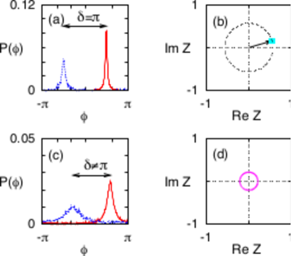
Specifically, there are three typical strategies for changing contrarians into conformists: (1) a fraction of contrarians is randomly chosen and then flipped into conformists; (2) contrarians are ranked according to the absolute value of their natural frequencies (). Then, they are flipped into conformists from the largest to a threshold , i.e. the coupling strength of the th oscillators will be if and otherwise. Therefore ; (3) the opposite of the process described in (2), i.e. if and otherwise, which leads to . Mathematically, the three strategies correspond to three different correlations between the coupling strength and the natural frequencies as follows:
| (79) |
| (80) |
| (81) |
where is the Heaviside function.
Reference [391] considers 1, and shows that the system has two types of coherent states: the state and the TW state (see Fig. 51). In the state, two clusters of conformists and contrarians keep a constant phase difference . The state is stationary, and the order parameter is a fixed point in phase space. For the TW state, the phase distribution spontaneously travels at a constant speed along the phase axis, always maintaining a constant separation . As a result, the order parameter traces a circle around the origin at a constant angular velocity.
As the control parameter varies, transitions are observed among the incoherent and the coherent states. The results can be split into two scenarios, depending on whether the conformists or the contrarians are more strongly affected by the mean field. Figure 52 reports the phase diagram when the contrarians are more strongly affected by the mean field, i.e. . For small , the system is dominated by contrarians, and therefore is in the incoherent state. Once exceeds a certain threshold, there are enough conformists for a consensus to emerge. At that point, the system jumps discontinuously to the state, where it is polarized into two groups (see Fig. 51(a)). Inversely, starting from the coherent state and adiabatically decreasing yields a discontinuous and hysteretic return to the incoherent state. On the other hand, if , the transitions become continuous. Typically, as increases from , the system goes from the incoherent to the state, then to the TW state, and finally settles on the state (see Fig. 3 of Ref. [391]).
Based on the Ott-Antonsen ansatz [241], the dynamics of Eq. (78) can be effectively reduced into a low-dimensional system describing the complex order parameters for the contrarians and conformists. By means of the analysis of the reduced system, the three steady states and their bifurcation points can be analytically obtained [391].
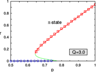
In Ref. [392], numerical simulations of 2 and 3 are presented, and both the state and the TW state are found. In a certain parameter regime of 3, furthermore, a special explosive behavior is taking place: when the control parameter is decreased to a critical threshold, the system bifurcates from the incoherent state into the TW state via a first-order like transition, while starting from the TW state, if increases, the order parameter exhibits a continuous and hysteretic return to the incoherent state (see Fig. 7(b) in Ref. [392]).
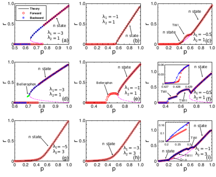
Recently, Qiu et al. provided a detailed and complete analytical treatment for model (78), based on linear stability analysis and mean-field analysis [393]. It has been proved that in this model the incoherent state is neutrally stable below the synchronization threshold, and the critical points for synchronization are derived for all the three cases. Moreover, all possible stationary coherent states in the model are predicted, including the state and the two types of TW states.
In Fig. 53, a detailed phase diagram characterizing the synchronization transitions in model (78) is reported. Depending on the correlations between the coupling strength and the natural frequencies (as well as on whether the conformists or contrarians are more strongly affected by the mean field), the system exhibits either first-order or second-order like transitions among different steady states. Besides the two examples of ES studied in Refs. [391] and [392] (which corresponds to Figs. 53(a) and 53(i), respectively) it is further revealed that a first-order transition can also occur in 2. As illustrated in Fig. 53(d), when increases, the system experiences a first-order transition from the incoherent state into the coherent state, i.e., the state. Inversely, when the system starts from the coherent state, as decreases, the system does not directly go back to the incoherent state. The state first bifurcates into a new coherent state named the Bellerophon state (see next Section for the full characterization of such a novel state) via a second-order transition. Then, as further decreases, the Bellerophon state loses its stability and the system jumps into the incoherent state via a first-order transition.
4.4 The Bellerophon state
In the previous Sections, a variety of coherent states emerging in the classical Kuramoto model have been discussed and characterized, such as the partially coherent state [237], the standing-wave [243, 335] and TW [243, 394] states, and the chimera state [395, 396, 217, 219]. In such coherent states, oscillators inside each one of them display typically frequency-locked patterns, and therefore behave like a giant oscillator as a whole. Here, instead, we describe the main properties of a recently discovered novel state: the Bellerophon state.
4.4.1 The Bellerophon state in frequency-weighted Kuramoto models
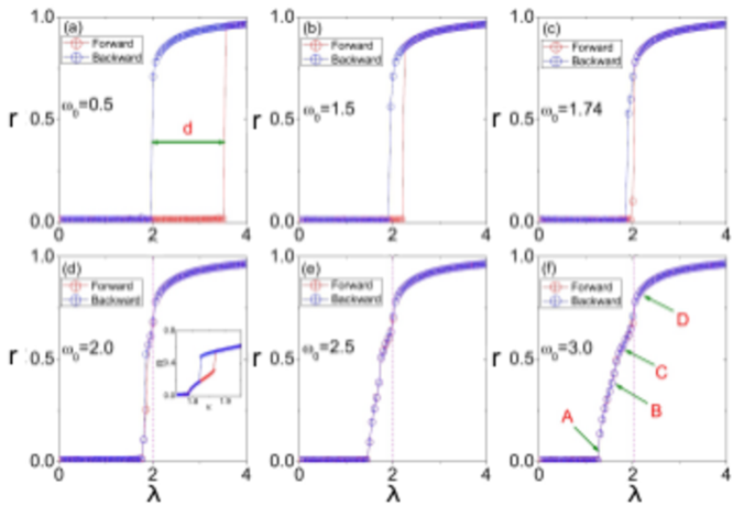
In Ref. [397], ES was studied in a frequency-weighted Kuramoto model
| (82) |
with a bimodal Lorentzian distribution
| (83) |
Here, and are the instantaneous phase and the natural frequency of the th oscillator, respectively, and is the coupling strength. is the width parameter (half width at half maximum) of each Lorentzian distribution, and are their central frequencies. As shown in Fig. (54), system (82) sustains both a first- and a second-order transition to synchronization. According to the theoretical analysis [373, 397], the critical point for the backward transition is always 2, while the critical point for the forward transition is
| (84) |
As the parameter increases, the characteristic hysteresis width shrinks, which induces eventually the conversion of a continuous transition to synchronization into an ES.
A new coherent state is unveiled in system (82), which is actually non-stationary and essentially different from all the coherent states studied before. In such a state, oscillators form quantized, time-dependent clusters, where neither their phases nor their instantaneous frequencies are locked. Their instantaneous speeds are different within the clusters, but they form a characteristic cusped pattern and, more importantly, they behave periodically in time so that their average values are the same. Given its intrinsic specular nature with respect to chimera states, the new state has been named the Bellerophon state in Ref. [397].
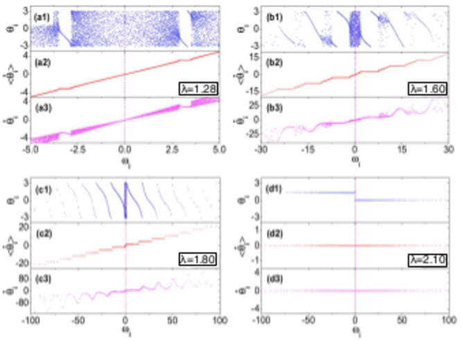
In Fig. 55 four typical steady states are illustrated, corresponding to the values denoted by letters A, B, C, and D in Fig. 54(f). Among them, Figs. 55(a)-55(c) are Bellerophon states while Fig. 55(d) is the fully coherent state. In Bellerophon states, oscillators form quantized clusters in terms of the average frequencies. The crucial point here is that although the average speeds of oscillators inside each cluster are equal to each other, their instantaneous speeds are generally different and quite heterogeneous. Furthermore, the instantaneous speeds of oscillators in each cluster are correlated and form the characteristic cusped pattern [Figs. 55(a3), 55(b3), and 55(c3)] analogous to that featured by the average frequencies of the oscillators within the chimera state. Therefore, inside each cluster, oscillators are neither phase- nor frequency-locked in a common sense. Rather, they seem to correlate in a higher order collective way: in terms of average speed oscillators inside each cluster are locked, but in terms of instantaneous speed each oscillator evolves uniquely. In fact, very interesting collective motion of oscillators can be observed in the unit circle, as illustrated in Ref. [397] (and, more specifically, in the animated movies which form part of the Supplementary Material of that Reference).
Bellerophon states can occur in system (82) also for different frequency distributions. For instance, in Ref. [398], model (82) was investigated with an asymmetric Lorentzian distribution:
| (85) |
where is kept as a constant, changes in order to shift the frequency distribution along the positive axis. It is found that in the intermediate regime between incoherence and full synchronization [398], the Bellerophon states emerge, as illustrated in Fig. 56. Furthermore, the evolution of oscillators exhibit periodic intermittency following a synchronous pattern of bursting in short periods and resting in long periods [398].
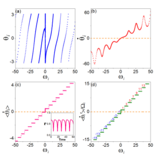
In Ref. [399], model (82) was investigated with a uniform frequency distribution:
| (86) |
It is revealed that, as the coupling strength increases, the system undergoes two transitions. First, a first-order phase transition occurs from the incoherent state to a Bellerophon state, and then the Bellerophon state bifurcates into the two-cluster synchronous state via a continuous transition, when the coupling strength further increases.
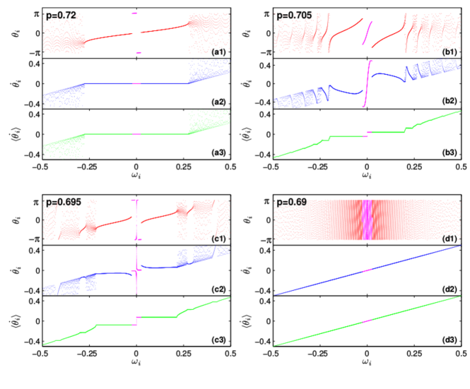
4.4.2 The Bellerophon state in coupled conformist and contrarian oscillators
The Bellerophon state is also observed in the model of Eq. (78), which is essentially different with respect to the frequency-weighted model (82). Let us focus on a typical example, namely that of Fig. 53(d). As the control parameter increases, the system experiences a first-order like transition from the incoherent state to the coherent state, i.e. the state. Inversely, when the system starts from the coherent state, as decreases, the system does not directly go back to the incoherent state. As shown in Fig. 53(d), the state first bifurcates into the Bellerophon state via a second-order transition. Then, as further decreases, the Bellerophon state looses its stability and the system finally jumps into the incoherent state via a first-order like transition. In Fig. 57, the typical Bellerophon states corresponding to Fig. 53(d) are characterized. Except for the fact that there are clusters of both conformists and contrarians, the observed Bellerophon states share all the other features of the frequency-weighted model described above.
4.5 Explosive synchronization in multi-layer networks
So far, our journey on explosive synchronization has been limited to the case of single-layer, or mono-layer, networks. Real complex systems, however, have far more complicated forms of interactions, which points to the fact that the hypothesis of a single-layer network may actually result an overestimation (or an underestimation) of the problem under study. A more accurate analysis resorts on multi-layer networks, and dynamical processes on top of them are attracting more and more attention (see, for instance, Ref. [249] for a recent and rather comprehensive review). Therefore, examining ES on multi-layer networks became a topic of the utmost significance.
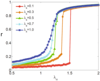
4.5.1 Multi-layer networks with the correlation property
Jiang et al. recently proposed a Kuramoto model on multiplex networks [400], which are composed of one SF network (as the base layer) and one community structured network (as the external layer), and where each node constructs local links with probability and long-range connections with probability (which is then the mixing parameter). Reference [400] mainly focused on how the coupling between layers affects the phase transition of oscillators in the based layer , for which the evolution equation reads as
| (87) |
where . The first and second terms are the same of those referring to a single-layer network, and only involve intra-layer interactions in the base layer . The third term accounts for the additional inter-layer interactions controlled by the coupling strength parameter . For simplicity, the hypothesis of symmetric coupling between both layers () is assumed, and is denoted by .
The inter-layer coupling plays a significant role in determining the phase transition of the base layer. As shown in Fig. 58, at weak coupling strengths () ES emerges. With increasing , however, the transition becomes more and more continuous: there is an interim period at , and a second-order-like transition occurs at , which indicates that strong inter-layer couplings hinder the emergence of ES.
Moreover, it was unveiled that other externalities (mainly the parameters and ) have great effect on ES. In details, increasing the mixing part puts off ES of the base layer, and requires larger critical coupling strengths , irrespectively of other parameters. This points is contrary to the findings in traditional modular networks [101, 284, 297], where long-range, inter-modular connections speed up the coherent state. As for coupling strength , its increase can accelerate ES of the base layer, though this effect seems to be very restricted.
4.5.2 Multi-layer networks with partial and weak correlation
A generative model of inter-dependent networks (including subnetworks and ) was proposed in Ref. [401]. At each time step, a node enters into both subnetworks, and constructs different links on each subnetwork. That is to say, nodes on both subnetworks have one-to-one interdependency with the same index. Then, like the preferential attachment rule in SF networks [402], the probability of producing one new link reads as and , where and control the mutual correlation between networks. It is clear that the connectivity of each layer depends on itself and its counterpart, and both subnetworks have the same power-law degree distribution.
The Kuramoto model is then introduced. Instead of a strong correlation, the natural frequency of oscillator in layer () is taken to be (), which means that the dynamics of oscillator is controlled by the local topology and connectivity of the other layer. Such a weak hypothesis of correlation can induce ES when and are sufficiently large. As and decrease, the abrupt transition is replaced by a continuous transition.
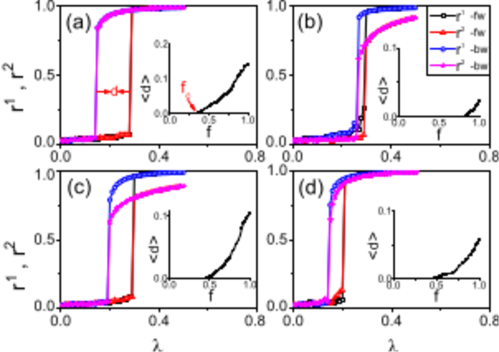
4.5.3 Multi-layer networks in the absence of correlation
Zhang et al. [21] proposed to consider the following system
| (88) |
where the new parameter accounts for an adaptive control of nodes.
Initially, a fraction of the nodes is randomly chosen, and is assumed for each of the selected nodes, where is the instantaneous local order parameter of the -th oscillator, defined as , and denotes the phase averaged over the ensemble of neighbors. For the remaining fraction of the nodes, . Obviously, returns the traditional Kuramoto model [23, 237, 238, 295], while indicates that a fraction of nodes are adaptively controlled by the local order parameter. Besides, another significant point is the choice of the natural frequencies of oscillators, which are taken from a random homogeneous distribution in the range . Based on these assumptions, it was reported that an abrupt (with a hysteresis loop) transition takes place if is over a critical value . Namely, the absence of correlation features can also promote the occurrence of ES in single-layer networks.
In order to explore the case of inter-dependent networks, Ref. [21] extended the analysis to the situation where each node has a one-to-one partner with the same index . The equations become
| (89) |
where the superscripts and denote the network layers 1 and 2, and involve the coupling of two layers via dependency links. In details, if nodes fall into the fraction , and refer to the local order parameters and , i.e. and ( otherwise), where and . The frequency function is still random homogeneous and in the range , while can change from a random to a Lorentzian distribution.
Figure 59 shows the dependency of synchronization levels and on for different choices of the layer 2 and . ES occurs and seems very robust against the difference in topology and frequency distribution, which indicates that the correlation between oscillator’s frequency and node’s degree is not the essential condition for the emergence of ES. If is below the critical value , synchronization returns to a second-order transition. More importantly, these observations can be quantitatively verified via the mean-field theory. In the traditional second-order transition, oscillators with close frequency firstly collapse into small synchronization clusters, which gradually converge towards a giant cluster at the critical coupling strength. However, under ES, small clusters are prevented and all free oscillators are abruptly attracted to the giant cluster. Recently, furthermore, this kind of ES has been shown to coexist with the standard phase of the Kuramoto model in the thermodynamic limit [403].
5 Applications
5.1 Explosive percolation in real physical systems
Most of the studies on Explosive Percolation reviewed in Section 2 are explicitly conducted in the thermodynamic limit, i.e. under the hypothesis of an infinite system size (or a size of the order of the Avogadro’s number, ). However, real world systems are always finite-sized. For instance, the Internet, world-wide airline network and online social networks (just to mention three examples of very large sized real networks) have all values of considerably smaller than [27]. In this sense, it is interesting to reveal how the AP process may induce significant discrete jumps in the realm of real-world networks, where EP is generally considered to be a phenomenon of cascading failures [106, 94].
One of the major events of electrical blackout was affecting much of Italy on 28 September 2003: the shutdown of power stations directly led to the failure of nodes in the Internet communication network, which in turn caused further breakdown of power stations. This iterative process of cascading failures can also occur in a single power-grid network such as the blackout in Northwestern America in August 1996, and the blackout in Northeastern America and Canada in August 2003, where one overloaded node caused other nodes to also become overloaded and thus disabled the entire network. Other examples include the financial crises (in the network of global financial market) and the spreading of information and rumors through online social networks, such as Facebook or Twitter, where a failing node can cause its neighbors to fail as well. A common feature of these cascading failures is that they represent an inverse process of EP, which has a devastating effect on the network stability, and may cause huge economic losses.
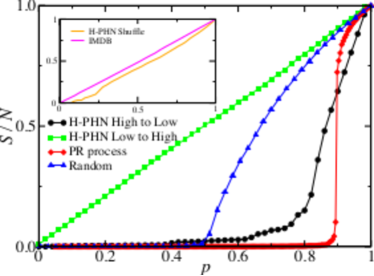
Although a general answer to the question of how to suppress or control a cascading failure in real systems is still missing, some progress in this direction has been achieved [50, 58, 10, 85, 404, 113, 45], illustrating how the AP rule can actually be used in real systems.
For example, Rozenfeld et al. considered EP in the human protein homology network (H-PHN) and showed that the emergence of a spanning cluster exhibits similar features to a AP process [50]. Their results indicate that the evolutionary-based processes shaping the topology of the H-PHN through duplication-divergence events may occur in sudden steps, similarly to what is seen in first-order like phase transitions.
Cho et al. considered the diffusion-limited cluster aggregation (DLCA) model of the sol-gel transition, and found that a discontinuous percolation transitions can be observed when particles are Brownian, in which cluster velocity depends on cluster size as with [10, 85].
Pan et al. considered social networks community structures and assortativity (such as a mobile phone call network and a large arXiv coauthorship network), and found that the percolation transition depends on the structural properties of the network [58].
Oliveira et al. discovered that the electric breakdown due to pollution with metallic powder can become explosive if the inhibition of adsorption due to a local electric field becomes too strong [113].
Later on, Radicchi considered the case of coupled networks and found that the dependency links have an important role in the phase transition [404]. For a high density of dependency links, the network disintegrates in a form of a first-order phase transition, whereas for a low density of dependency links, the network disintegrates in a second-order transition. In the following, we briefly linger in each one of these cases.
5.1.1 The human protein homology network
First, we discuss the case of H-PHN. Based on real data111The H-PHN was obtained from the Similarity Matrix of Proteins (SIMAP) project, http://boinc.bio.wzw.tum.de/boincsimap, Rozenfeld et al. found that H-PHN is composed of highly connected clusters of homologous nodes, while links between nodes of low homology generate inter-cluster connections, which is similar to the presence of strong links within communities and weak links between communities [50]. Further, they found that H-PHN is a weighted modular network, with the weights denoting the degree of similarity (homology) between two proteins. Ref. [50] claimed that such a weighted modular network can be explained on the basis of a product rule (PR) model. The idea is the following: suppose that H-PHN is grown up from a spanning skeleton of the network which connects all the different network areas. A new protein has a much larger weight to generate links within a module rather than with proteins that are further away. These dense modules are then connected with each other through weaker links. In the terminology of the PR model, this corresponds to an increased probability of connections between small clusters, if compared to the growth of already large clusters.
A quantity is introduced to detect the degree of similarity between two optimally aligned proteins [50]. indicates a perfect alignment between the two proteins, or in other words, a short genetic distance between the proteins. The values of for a protein pair in the network is taken to be the weight of the corresponding link. Then, the concrete process to construct the H-PHN can be implemented by considering an empty network of all proteins, and adding one link at a time in decreasing order of the weight, quantified by . The process initially leads to well-connected families of highly homologous proteins, that are inter-connected at later stages by links with smaller values of , resembling the requirements for EP in Ref. [9].
The results are reported (black line with “circles”) in Fig. 60. represents the fraction of nodes in the largest cluster of the H-PHN, and denotes the percentage of links. One clearly sees that the largest cluster in the network remains small until reaches , and then quickly increases for . The behavior is very similar to an AP, i.e. links are added locally and without a significantly large spanning cluster before , while the subsequent addition of links after causes the small clusters to merge into a spanning entity. For comparison, the red line with “diamonds” in the same figure shows the results of a pure AP, for the same number of nodes. One sees that the two curves have a high-degree similarity, and the PR model has a sharper transition than the H-PHN.

For a deep understanding of the nature of the transition, Rozenfeld et al. reported the results for the cases of adding links in increasing order of (green curve with “squares” in Fig. 60) and adding links randomly (the blue curve with “triangles” in Fig. 60). The former strategy induces a percolation transition at a very early stage, and the largest cluster increases linearly with , i.e. almost every new link attaches to the largest cluster. In the latter strategy, the largest component remains small before its critical point , and then increases approximately linearly after , i.e. following a second-order transition. By comparison of all the four curves in Fig. 60 one concludes that the case of decreasing weight in the H-PHN is much steeper than the case of random addition, and is much closer to the case of PR processes, indicating that the evolution of a modular network can be explained through the idea of EP.
The sharp transition of the H-PHN is not a universal property ascribed to weighted networks. The inset of Fig. 60 shows that, when the link weights of the H-PHN are shuffled without modifying the structure of the network, a smooth percolation transition is observed at an early stage. Similar growth patterns can be observed in other modular networks, such as the network of movie actors from IMDB in which two actors are connected if they co-acted in a movie (see the inset of Fig. 60).
5.1.2 The DLCA model
As a second case, we briefly discuss the case of the DLCA model. Initially, single particles are placed randomly in a square lattice. Assume that the particles are Brownian and the cluster velocity depends on the cluster size as . For convenience of numerical simulations, one first lets the velocity of a cluster be inversely proportional to the square root of its size. The simulations are performed as follows: at each time step, (i) a -sized cluster is selected with the probability , and is moved to the nearest neighbor, where is the number of -sized clusters. When two distinct clusters are placed at the nearest-neighbor positions, these clusters are regarded as being merged, forming a larger one. (ii) The time is advanced by . Steps (i) and (ii) are repeated until the network percolates.
Let be the number of cluster aggregation events per total particle number. Whenever two clusters merge, is increased by . Since aggregation events occur during all aggregation processes, the aggregation event stops at [10]. Figure 61(b) shows the dependence of the giant cluster size on . One sees that it increases drastically, exhibiting a discontinuous phase transition. For comparison, the dependence of on is shown for the original DLCA model in Fig. 61(a), where sees that increases monotonically with . The different behavior between Figs. 61(a) and (b) is caused by the nonlinear relationship between and , as shown in the inset of Fig. 61(b). When is small, increases almost linearly with . At variance, as approaches , increases drastically in a power-law manner, resulting a discontinuous phase transition.
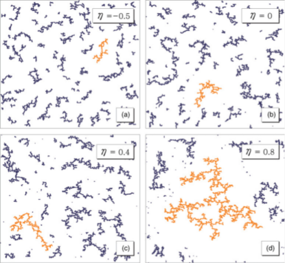
Let us now move to the general case of . Here, a cluster is picked up with a probability proportional to while the other rules in the numerical simulations are held. When clusters merge, is increased by . The time is given by . Intuitively, when is small or negative, fewer large-sized clusters are selected, so that their growth is suppressed. Medium-sized clusters are abundant even close to , and they merge suddenly, resulting in a discontinuous transition. In contrast, when is positively large, larger-sized clusters are selected and they have larger chances of colliding with other ones, merging into a bigger cluster. The result is that these latter clusters can grow faster than smaller ones, so the giant cluster grows continuously and the transition becomes continuous. The presence of a tri-critical point is expected across which the transition type is changed. Figure 62 shows snapshots of the system for different values of at , supporting the above arguments.
The DLCA model was later extended to a reaction-limited cluster aggregation model in which clusters diffuse following Brownian motion, and when two clusters come into contact with each other, they merge with a certain probability and remain separated with the remaining probability [85]. It is found that a discontinuous transition can be observed in two and three dimensions, while the transition remains continuous in four dimensions.
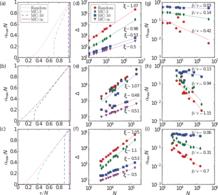
5.1.3 Social networks
Next, we linger on the case of social networks [58], such as the empirical mobile phone call (MPC) network, and a large arXiv coauthorship (CA) network, where the nodes represent people and links denote their interactions. These social networks share common features such as community structures and assortativity.
The MPC data consist of voice calls over a period of days. An aggregated undirected weighted network can be constructed, where edges represent bidirectional calls between users and weights represent the total number of calls. The largest connected component (LCC) is then extracted, with nodes and edges.
The collaboration data is from the arXiv 222http://arxiv.org and contains all e-prints in “physics” until March 2010. There are article headers, from which one extracts the authors. In the CA network two authors are connected if they signed together articles whose number determines the link weight. The LCC is extracted, with nodes and edges. In addition, a filtered version of the CA can be constructed, where articles with more than authors ( of the total number) are ignored. This is to remove the very large cliques from papers with authors in fields such as hep-ex or astro-ph, where the principles behind collaboration network formation appear different. The LCC of the resulting smaller CA network has nodes and edges. Note that, although the number of nodes is not much smaller than for that of CA, the number of edges is an order of magnitude smaller.
For describing the percolation process, Pan et al. used the min-cluster (MC-) SR, with different values of [58]. Initially, all the edges of the empirical network are considered unoccupied. Then, at each time step, unoccupied edges are drawn at random. Out of these edges, the one minimizing the size of the component formed if it were occupied is chosen. Intra-component edges are always favored against inter-component edges, as they do not increase the size of any cluster. When comparing two inter-component edges, the one for which the sum of cluster sizes that it connects is minimized is selected. As intra-cluster edges do not affect cluster growth, one considers only the number of inter-cluster edges . In particular, three variants of the MC rule (MC-2, MC-10, and MC-) as well as random link percolation are compared [58]. Figures 63(a), (b) and (c) show the variation of the fraction against the scaled number of inter-component edges, . For all the three networks, the transition of the order parameter is smooth for the random case, while for the extreme case, MC-, the transition appears abrupt. For MC-2 and MC-10, the situation is more complicated, and in the following will be described in more detail.
One can study the dependence of the width of the transition window on the system size, where and are the lowest values of for which and , respectively [9]. In general, the width scales as a power law with the system size (). For classical percolation, . It is argued that for EP, and the rescaled width of the transition region () vanishes in the limit of large . In order to apply finite-size scaling to empirical networks, samples of different sizes are needed. As call networks are geographically embedded, one extracts sub-networks of users in chosen cities, based on postal codes of their subscriptions. For the CA networks, one extracts sub-networks of authors with articles in the same subject class. It turns out that, for all networks , with for random and for the MC- case (see Figs. 63(d), (e), and (f)). Thus, the exponent clearly differentiates the explosive transition from random-link percolation. Furthermore, for all three networks, for the MC-2, resembling an ordinary percolation transition. However, for MC-10, the scaling exponent behaves differently for the three networks. For the MPC and smaller CA networks, , indicating EP. For the CA collected data points seem to indicate that there is no scaling. However, a closer inspection shows that they cluster around two straight lines with and .
According to Ref. [34], the order parameter has a finite-size scaling
| (90) |
where is some universal function, is the control parameter, is the critical point of the transition, is the critical exponent of the order parameter, and is another critical exponent. One chooses the critical value of the control parameter as the value of where the susceptibility (that is, the average cluster size) has its maximum. For the MPC network [Fig. 63(g)], the scaling at of yields a very small exponent for the MC-10 case, while for MC-2 and random percolation, the exponents are larger ( and , respectively). The exponents for the SCA network behave similarly [Fig. 63(h)] with a low value for the MC-10 case and relatively high values and for MC-2 and random percolation, respectively. In contrast, for the CA network, the exponents have higher values for all cases [Fig. 63(i)] (, , and ) for MC-10, MC-2, and random percolation, respectively.
5.1.4 Inter-dependent networks
Recently, percolation in real systems was extended to the case of inter-dependent networks [404]. The functioning of a real network depends not only on the reliability of its own components, but also on the simultaneous operation of other real networks coupled with it. Percolation transitions in inter-dependent networks can be understood by decomposing these systems into uncoupled graphs: the intersection among the layers, and the remainders of the layers. When the intersection dominates the remainders, an inter-connected network undergoes a smooth percolation transition. Conversely, if the intersection is dominated by the contribution of the remainders, the transition becomes abrupt even in small networks.
As an example of real systems, Radicchi showed the transition for two inter-connected systems of interest in the biology: the H. sapiens protein-protein interaction network and the C. elegans connectome, finding that the inter-connected systems undergo smooth percolation transitions [404]. The reason is that these organisms have developed inter-connected networks sharing a core of “high quality” edges to prevent catastrophic failures. The same properties seem to characterize also the multi-layer air transportation network within the USA major airports, where the set of “high” quality’ edges that avoid truly catastrophic changes in the connectedness of the entire inter-dependent system are constituted.
5.2 Explosive synchronization in real physical systems
5.2.1 Power grids
Among the many real-world systems where ES can be observed, power grids are actually the ones in which cascading of failures has been experienced for numerous times.
One way to produce a cascade of failures is by the overload of lines: an outage of a line may lead to overload on other lines, thereby eventually leading to their outage. For instance, in August 2003, an undetected initial power line failure in Ohio caused a massive power blackout rolled across Northeastern USA and Canada, spanning eight states and two provinces, and affecting some 55 million people [405].
Another way is overloading the power stations: an outage of a node may lead to overload on other nodes, also leading to their outage. For example, a small initial power shutdown in El Paso (Texas) caused the August 1996 blackout in Northwestern America in which the power outage spread through six states between Oregon and California, leaving million customers without electricity.
Around the world, the number of outages affecting large populations has steadily risen in the past decades, causing enormous economic losses.
The cascade of failures in power grids can be also explained in terms of their underneath inter-dependent network structure. For example, in September 2003, Italy was affected by a country-wide blackout: the shutdown of power stations directly led to the failure of nodes in the Internet communication network, which in turn caused further breakdown of power stations and left 57 million Italians in the dark [106].
Large-scale and/or long term failures have devastating effects on almost every aspect in modern life, and especially on inter-dependent systems (such as telecommunication, gas and water supply, and transportation systems). The iterative process of cascading failures can be described by the scheme of Fig. 64 where the outbreak in panel (d) is initiated by the node failure in panel (a) through a few intermediate steps [94].
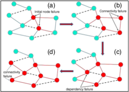
A power grid is a network where links are power lines and nodes may be either generators (power plants) or consumers. The generators produce the electric energy which needs to travel long distances in high-voltage transmission lines (e.g. 400 kV) in order to arrive the consumers or loads [406, 407, 408, 409]. The nodes may therefore consume, produce or distribute power, whereas the links transport power and may include passive elements with resistance, capacitance and inductance. A power grid is embedded in a 2D real space. Figure 65 is a representation of the Northern European power grid with nodes and connections [410].
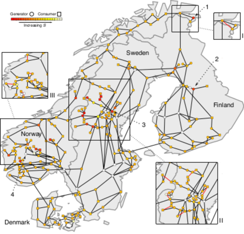
A fundamental requisite for a power grid to operate in a stable way is the maintenance of a phase-locked state within the entire system, thus synchronization is understood as the ability of a power grid to keep a global state where generators and loads (with intrinsic different frequencies) run with the same effective frequency (e.g. 50/60 Hz). If loads are too strong (or unevenly distributed) or if some major fault (or a lightening) occurs, a node may lose synchronization. In that situation, the synchronization landscape may change drastically and a blackout may occur.
Therefore, power grids are generally planned and operated to withstand the occurrence of certain disturbances. For this purpose, the following conditions of dynamic security are being guaranteed [407]: 1) when any of a specified set of disturbances occurs, the system survives the ensuing transient and moves into a steady-state condition; 2) no bus voltage magnitudes during transients are outside their permissible ranges; 3) in this new steady-state condition, no control devices, equipment or transmission lines are overloaded and no bus voltage magnitudes are outside their permissible ranges (say of nominal).
Now, it happens that a power system is continuously experiencing disturbances, such as outages, short-circuits, sudden large load changes, or a combination of such events. Because of economic and environmental pressures, power grids tend to run at their full utilization, which increases the effects of these disturbances on their security. For example, when several voltages collapse, a power system must operate even closer to the limits of stability and then the risk of a major breakdown is increased [409].
Several models have been proposed to analyze the stability of power grids [411, 412, 239, 408, 413, 406, 414]. In these models, each node- has the same equation of motion, and is characterized by a parameter quantifying the generated () or consumed () power. The state of each node is determined by its phase angle and velocity . During regular operations, generators and consumers run with the same frequency Hz or Hz. The phase of each node- is then written as
| (91) |
where is a phase fluctuation.
For simplicity, one may assume that the nodes can be modeled as having the same dissipative coefficient , the same moment of inertia, and that power is not lost during transmission. By energy conservation, each generated or consumed power must be equal to the sum of the power taken from the grid () plus the accumulated () and dissipated () power, i.e.
| (92) |
Now, during its rotation a turbine dissipates energy at a rate proportional to the square of its angular velocity [408]
| (93) |
and it accumulates kinetic energy at a rate
| (94) |
where is the moment of inertia. The condition for power transmission is that the two devices do not operate in phase, i.e. there is a phase difference between the two nodes connected by a line . The transmitted power is proportional to the sinus of the phase difference between the voltages of the nodes at the two end-points of the line [413], which gives
| (95) |
where is an upper bound for the transmission capacity of a line. Substituting Eqs. (93), (94) and (95) into Eq. (92) one has
| (96) |
which can be written into normalized units as
| (97) |
where and are the normalized parameters, and are the elements of the adjacency matrix which accounts for the heterogeneity of the network. is related to both generated and dissipated power at the node, while (the strength of the coupling) is related to the maximum transmitted power. Eq. (97) is the basic equation considered in power grids dynamics. Notice that, when the inertia is negligible, one may ignore the term in Eq. (97), which then returns to the classical 1970 Kuramoto model.
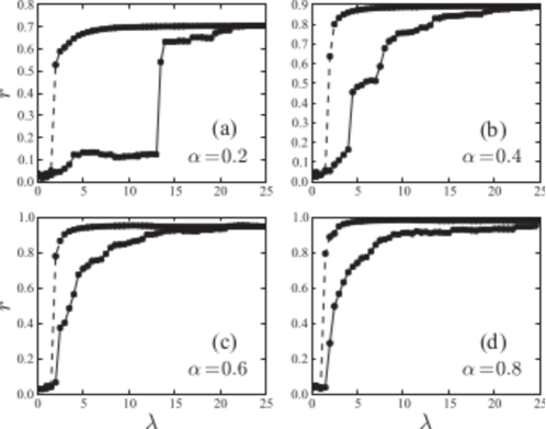
In addition to load balance, synchronization between all elements of the grid is a crucial aspect to the system. Recently, ES in Eq. (97) has been extensively studied [415, 416, 417, 418]. The stable operation of a power grid requires that all machines run at the same frequency . The phases of the machines will generally be different, but the phase differences are constant in time. To study the influence of dynamics and structure on global synchronization, is generally assumed to satisfy a distribution with zero average. For example, can be explained as the natural frequency of node , and assumed to be of the form [415, 417, 418]
| (98) |
where is the degree of node , the network average degree, and a proportionality constant. That is, the natural frequency of a node is assumed to be proportional to its degree.
The choice of Eq. (98) assumes that, in SF topologies, many nodes play the role of consumers (nodes with ), while nodes with high degrees play the role of power producers (nodes with ). In this framework, the relation is satisfied, which means that the total consumed power is equivalent to the total generated power. In this latter case, all oscillators try to rotate independently at their own natural frequencies, while the coupling tends to synchronize them to a common phase. Besides the degree distribution , it is know that real world network can display either assortativity or disassortativity degree mixing behavior. When degree-degree correlations are accounted for, it is found that the synchronization diagrams have a strong dependence on the network assortativity, indicating that one is able to control the hysteretic behavior of the second-order Kuramoto model by tuning the network properties [415].
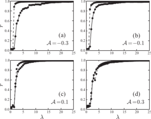
In numerical simulations, all the initial networks are constructed through the BA model with and . Equation (97) is integrated and the Kuramoto order parameter (Eq. (14)) is calculated after a transient process. Figure 66 shows the forward and backward synchronization diagrams for different values of within the interval . Panels (a)-(d) represent the cases of and , respectively. It is easy to see that there is a hysteresis loop in all the four cases, indicating that ES is taking place in the network. From Fig. 66 we also see that the area of hysteresis and the critical coupling for the onset of synchronization in the forward branch tends to decrease as is increased, which also contributes to increase the maximal value of the order parameter.
The network’s degree-degree correlations can be quantified by the assortativity coefficient defined in Eq. (42). In order to inspect the influence of network’s degree-degree correlation on ES in Eq. (97), one needs to change the assortativity of the network, which can be implemented as follows [415]: at each step, two edges are selected at random and the four nodes associated to the selected pair of edges are ordered from the lowest to the highest degree. Given a target assortative mixing (), with probability a new edge is formed between the first and second nodes and another one between the third and fourth nodes. If one of the two new edges already exists, the step is discarded and a new pair of edges is chosen. A similar heuristic mechanism can also generate disassortative networks (). Figure 67 shows the synchronization diagram for networks with different values of assortativity, where panels (a)-(d) represent the cases of and , respectively. As increases, the hysteresis becomes smaller and smaller, and the critical coupling of the increasing branch is weakly affected.
The natural frequencies can also be chosen from different distributions. For instance, Olmi et al. considered the case of a Gaussian distribution with zero average and unitary standard deviation [416]. It is observed that, in the hysteretic region, clusters of locked oscillators of various sizes and different levels of synchronization coexist.
It is important to remark that the process of ES in Eq. (97) is quite different from that of the Kuramoto model. It is revealed that in the case of uncorrelated SF networks, nodes join the synchronous component progressively, grouped into cluster of nodes with the same degree, starting from small degrees. The phenomenon was therefore called cluster explosive synchronization [417, 418], and the difference with the case of the Kuramoto model is that in the latter the average frequency jumps to for all at the same time. Figure 68 reports the synchronization process and highlights the progressive presence of clustering.
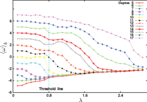
5.2.2 Smart grids
An imperative condition for the reliable functioning of power-grids is that the generators remain synchronized. This condition is relatively easy to be attained in traditional power grids, where the power plants are mainly based on coal, gas, oil or nuclear power. However, in recent years, more and more distributed energy sources and self-sufficient micro-grids are included in the network, such as wind turbines, photovoltaic arrays, bio-gas power generators, and other renewable energy sources. Such modern grids often consist of thousands of power substations and generators linked across thousands of kilometers, and are therefore much larger (and more complicated) than the traditional ones.
They are called smart grids, because they make use of information and communication technologies (ICTs) to collect information (such as the behaviors of suppliers, consumers, and prosumers) and to take actions in an automated fashion to improve the efficiency, reliability, economics, and sustainability of the production and distribution of electricity [419, 406, 412, 414, 413].
A key problem of smart grids is their stability. For instance, any person who has a solar panel at home, may become an energy trader, i.e. buy energy when the price is low, store it and then resell when the price is high, resulting in a new market within smart grids. As markets are known to be unstable, their influence to power grids is serious. Another element of instability is the fluctuation of renewable energy sources, as for instance wind turbines which depend significantly on the environment and season. All these factors introduce disturbances and fluctuations in production and demand, which may trigger desynchronization of power generators. Once it happens, the connected generators cannot be in pace and thus induce a cascading failure, which may be the reason behind the increasing number of power blackouts reported in recent years.
A characteristic feature of smart grids is their large fluctuations in energy. Notice that in the case of traditional power grids, we have a balance between the generators and the consumers, i.e. from Eq. (98) we have . However, in the case of smart grids, this balance may not hold, and thus one has
| (99) |
In the following, without loss of generality, we describe the case of .
The simplest non trivial grid is a two-element system consisting of one generator and one consumer [412]. In the phase-locked state, both derivatives and are zero, and from Eq. (97) one has
| (100) |
For the sum over all the equations gives,
| (101) |
Therefore, the system can only reach equilibrium when Eq. (101) is satisfied, i.e. when . When instead , one defines and , with being the coupling strength. Equation (97) can be then rewritten as
| (102) |
where and . Figure 69(a) shows the case of , where there are two fixed points. One fixed point is stable and the other is unstable, therefore all trajectories converge to the stable fixed point. Figure 69(b) shows the case of , where there are no fixed points, and all trajectories converge to a limit cycle. Figure 69(c) shows the case of , where the fixed point and the limit cycle coexist such that the dynamics depends crucially on the initial conditions. Figure 69(d) shows the parameter space of the systems. The majority of power grids are operating close to the edge of stability, i.e. in the region of coexistence, at least during periods of high loads [412]. Therefore, the dynamics depends crucially on the initial conditions, and static power grid models are yet insufficient to fully capture the complexity of the system.
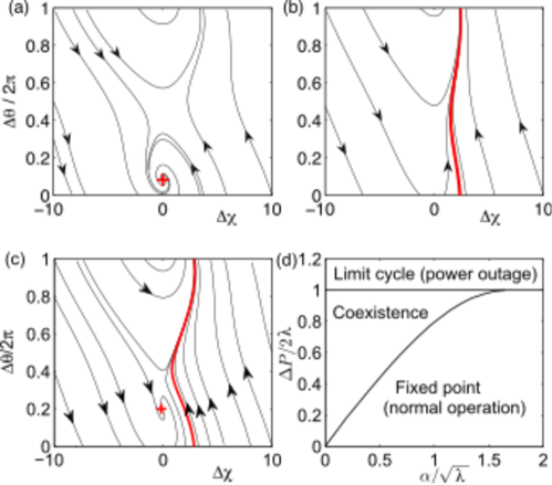
5.2.3 Brain dynamics
Synchronization plays an important role in sustaining basic brain functions such as emotions, complex thoughts, memory, language comprehension, consciousness, etc. [420]. For instance, the importance of synchronization of oscillatory phases between different brain regions in memory processes has been demonstrated [421]. On the other side, clinical evidence points out that abnormal synchronization of a small group of neurons may result in ruining some of the brain functions, leading to pathological behaviors such as Parkinson disease, tremor, and epilepsy.
Let us take epilepsy as an example. The disease manifests itself with recurrent unprovoked seizures resulting from a wide variety of causes, and is also the world’s most prominent serious brain disorder. Unless other neurological problems exist, patients with epilepsy typically have normal neurological function in between the seizures. Understanding the transition between the normal function and the seizure is useful for both improving the treatment of epilepsy and providing early warnings to patients.
Epilepsy has four phases: the interictal period, the onset of the seizure, and the propagation and termination phases. It is found that the coupling between brain areas during seizures changes with time, increasing or decreasing at the seizure onset in different cases [422]. At variance, when seizure termination is approached, the coupling of brain activity always increases. Both the onset and termination processes are very fast, indicating a jumping phase transition at critical coupling. The sudden emergence and termination of seizures suggested therefore that ES may play a role [423].
A seizure originates in a focal region, and then spreads to other brain regions. The individuation of the focal region from which an epileptic seizure is originated was performed in Ref. [424] in terms of phase synchronization indicators. During seizures, there is an overall increase of synchrony between the thalamus and temporal lobe structures. The phenomenon of seizure can be studied by means of a network approach, where a node can be either an individual neuron, or a population of neurons within a given structure, or an entire brain structure or region [423].
Guye et al. selected thirteen patients undergoing pre-surgical evaluation of drug-resistant temporal lobe epilepsy, and checked their recordings of intracerebral electrodes [425]. Figure 2 of Ref. [425] reveals that, during the seizure, synchronization values are significantly higher than those of the background period, indicating a jumping transition. The abruptness of the transition in the seizure has been also confirmed by many other studies [422, 423, 426, 427].
Another example is the anesthetic-induced unresponsiveness, which may result from specific interactions of anesthetics with the neural circuits regulating sleep and wakefulness. One common belief is that emergence from anesthesia is the inverse process of induction. Friedman et al. made experiments on transitions between conscious and unconscious states [428]. By generating anesthetic dose-response data in both insects and mammals, Ref. [428] demonstrated that the forward and backward paths through which anesthetic-induced unconsciousness arises and dissipates are not identical. Instead, a hysteresis is exhibited that isn’t fully explained by pharmacokinetics, as previously thought. Figure 70 shows the results for both the cases of path-dependent (a) and path-independent (b) state transitions. In particular, Fig. 70(a) displays a hysteresis loop, in contrast to the common belief.
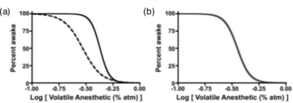
Joiner et al. provided further experimental evidence of the existence of hysteresis in the anesthetic-induced unresponsiveness [429]. The study proposes that processes selectively contributing to neural inertia may be impaired in pathophysiological conditions. Certain features exist in a minimal neural circuit that underly neural inertia, and can be used to model the dependence of anesthesia on feedback bistability. Figure 71 represents a sketch of the models from Ref. [429]. The sketch (a) is a simple kinetic model describing the transitions between two states, one unbound and the other bound to drug; (b) is the resulting dose-response curves for the forward and reverse reactions; (c) is the bistable situation where distinct feedback mechanisms are activated to shift drug sensitivity toward stabilization of the state; and (d) is the hysteresis in dose-response curves for anesthesia induction and emergence.
Kim et al. recently hypothesized that the conditions for ES in human brain networks would be present in the anesthetized brain just over the threshold of unconsciousness [430]. To test this hypothesis, Ref. [430] constructed functional brain networks from multi-channel electroencephalogram recordings in seven healthy subjects across conscious, unconscious, and recovery states, and demonstrated for the first time that the network conditions for ES (especially the suppressive rule of Ref. [19]) are present in empirically-derived functional brain networks.
Together with the experimental studies for the hysteresis loop in brain functioning, some theoretical works have also tried to understand the underlying mechanism of ES in neural systems [63]. For instance, Chen et al. investigated the property of phase synchronization transition of coupled FitzHugh-Nagumo oscillators in BA SF networks, and reported the existence of ES. The model reads as
| (103) |
where , , and and are the fast and the slow variables, respectively. The parameter describes the excitability of the th unit. If , the system is excitable, while implies that the system is oscillatory. are the elements of the adjacency matrix of the network, is the coupling constant, and is a Gaussian noise that is independent for different units and satisfies and with noise intensity , and . The natural frequency is assumed to be an increasing function of the degree , by taking as follows
| (104) |
where and are the maximum and minimum degrees in the network, respectively. The factor determines the slope of the linear expression. The larger is , the wider the distribution of .
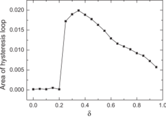
The synchronization diagram can be obtained by performing both the forward and the backward simulations. Chen et al. showed that, for BA networks, the nature of synchronization transition drastically changes with [63]. When is relatively small, the synchronization transition is continuous. Increasing to a middle value, one can see that as increases the order parameter abruptly jumps from to at , and therefore a sharp transition takes place at the onset of synchronization. On the other hand, the curve corresponding to the backward simulations also shows a sharp transition from the synchronized state to the incoherent one at . The two sharp transitions occur at different values of , determining a strong hysteresis loop. To measure the influence of on ES, Chen et al. calculated the area of hysteresis loop, and found that, increasing further to , the first-order nature of the phase transition is still present, but the area of the hysteresis loop becomes smaller [63]. Figure 72 shows how the area changes with : one can see that the area vanishes when , implying that the synchronization transition is there of second-order type. When is increased to , this area drastically changes to a non-zero value, indicating that the transition changes from a second-order type to a first-order one at around . With further increasing , this area shows a non-monotonic dependence on , and a maximum area occurs at .
5.2.4 Biological systems
Together with the example of the FitzHugh-Nagumo model of Eq. (5.2.3), other models of relevance for biological systems have been shown to display ES. Recently Chen et al. [76] reported that ES (as well as frequency-degree correlation properties) can take place in a very wide range of oscillatory networks, without any particular structure constraint. In Ref. [76], diffusively coupled SF networks of complex Ginzburg-Landau oscillators (CGLE) [431] are used,
| (105) |
where is the oscillator’s natural frequency, is a dispersion parameter. Both parameters are taken to be identical for all nodes. CGLE can generate rather complicated dynamics, including chaos, and different ways exist for the definition of frequency. In Ref. [76] the principal frequency of node () is defined as the value where the Fourier spectrum of a long time series of the dynamics of node has the highest peak.
Figures 73(a),(b) report the main results of the integration of Eq. (105). The principal frequencies of all nodes are there reported vs. the coupling strength . Panel (a) corresponds to the forward transition, panel (b) to the backward continuation. One observes a ES transition in the frequency domain. Before the transition, increasing of the coupling strength spontaneously induces a strongly inhomogeneous and well-ordered frequency distribution, with a positive correlation with the node degree. Defining the phase of node as , the authors compute also the phase order parameter . The result is shown in Fig. 73(c), where one notices the presence of a well pronounced hysteresis.

In Ref. [432] Bi et al. investigated explosive oscillation death in another well known model of amplitude oscillators. The oscillation death refers to the complete suppression of oscillations in coupled systems. This phenomenon has been extensively studied, both theoretically and experimentally [433, 434]. Ref. [432] considered a model of globally coupled Stuart-Landau oscillators with the frequency-weighted coupling term inspired by Ref. [61]:
| (106) |
where is a complex variable, and acts as the control parameter for the individual Stuart-Landau oscillator: the dynamics settles on a limit cycle if > 0, and on a fixed point if < 0. At variance with Ref. [76], oscillators here are not identical, and their natural frequencies are randomly taken from a frequency distribution .
Explosive oscillation dead was reported to occur in the solutions of Eq. (106). Fig. 74 shows a clear discontinuous jump in the forward and backward transitions for the order parameter . The inset reports the evolution of the variable for all the nodes at the transition point. It can be observed that not all the nodes collapse to the same fixed point.
5.2.5 Controlled laboratory experiments
Some few experimental evidences of ES have been given in controlled laboratory systems, which actually are of importance as they ultimately demonstrate the robustness and ubiquitousness of the phenomenon.
The first of these experiments was published by Leyva et al. in Ref. [16], and involved the search for explosive phase synchronization in frequency-degree correlated heterogeneous networks of electronic circuits. Initially, Ref. [16] performed numerical simulations of an ensemble of piece-wise linear Rössler units, interacting in a SF network via a bidirectional diffusive-like coupling [435, 436]:
| (107) | |||||
where the piece-wise linear part is given by
| (108) |
Every node (indexed by ) is here represented by an associated three-dimensional vector . The parameters are: , , , , and , where is a tunable quantity that regulates the dynamical state of the system. In particular, induces a chaotic dynamics in the range [435].
Finally, the natural oscillation frequency of node depends linearly on the parameter . To impose a degree-frequency positive correlation in this system, the values (and therefore, the oscillators’ frequencies) are distributed following the relation
| (109) |
where , and is a factor that determines the slope of the linear distribution. The range of frequencies in the ensemble becomes wider and wider as and (the maximum degree in the network) are increased, i.e. as more heterogeneous degree distributions (and/or steeper slopes) are considered.
Reference [16] shows that the system (5.2.5) gives rise to a ES transition, for an appropriate selection of the parameters. Precisely, the instantaneous phase for each oscillator is defined as , and the usual order parameter is monitored as a function of . The results are shown in Fig. 75(a), for a , SF network obtained by the BA growing algorithm for different values of the power-law exponent of the degree distribution. The inset reports the amplitude average synchronization error in the proximity of the transition for , and , to confirm that the system does not reach full synchronization when ES occurs.
The specific chaotic state of the nodes is a relevant variable, as it can be seen from the comparison (see Fig. 75(a)) of the case (black circles, second order phase transition) with the case (blue diamonds, first order phase transition) for . A more exhaustive description of ES emerges from the exploration of the full parameter space . The results are shown in Fig. 75(b), where the values of , for both forward and backward simulations are reported. As it can be seen, the plane can be clearly divided in two areas (denoted as and in the Figure) where the transition is of the first and second order, respectively. The striped portion of the area where the transition is of the first order marks the region where the hysteresis phenomenon is observed.
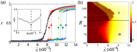
Motivated by the numerical study of Eqs. (5.2.5), Ref. [16] provided the first experimental evidence of ES, with the electronic network schematically shown in Fig. 76(a). The experiment consists of six piecewise Rössler circuits operating in the chaotic regime, which are labeled as , , …, . The details of the circuit construction, as well as the qualitative equivalence with the model of Eqs. (5.2.5) are available in Refs. [435, 436].
The circuits are arranged in a star-like configuration, which, on its turn, represents the maximally heterogeneous structure available for small ensembles. All the chaotic oscillators have the same internal , to ensure that they work in an almost identical dynamical regime. By a fine tuning of the values of the capacitors, circuits are configured such that the central node oscillates with a mean frequency of Hz, and the leaves nodes , …, are set with frequencies in the range of Hz. Notice that, due to the experimental variability, the frequencies of the oscillators suffer also from unavoidable dispersion.

Once the data are stored, processing of them is made to obtain the equivalent instantaneous phases. These latter quantities are calculated by defining the instantaneous phase of each oscillator as in each interval , where is the instant at which the crossing of the -th oscillator with its Poincaré section occurs. Fig. 76(b) reports the experimental synchronization diagram for three values of the parameter , both for forward and backward variations of the coupling strength . As in the numerical case, the dynamical regime tuned by determines whether the transition is of the first or second order.
Experimental evidence of ES has been recently given also in coupled chemo-mechanical systems, and more specifically in mercury beating-heart (MBH) oscillators [437]. Ref. [437] considered a star network configuration, where a central MBH oscillator is connected with other three MBH leaves oscillators. Furthermore, the experimental parameters are tuned properly, in a way that the natural frequencies of each oscillator is proportional to the number of its links. Not only Ref. [437] gives evidence that a gradual increase of the coupling strength results in an abrupt and irreversible (first-order like) transition, but it also proved how to engineer magnetic-like states of synchronization, by the use of an external signal.
5.2.6 Control of explosive synchronization
A characteristic feature of continuous phase transitions is that after the transition point, the order parameter increases gradually with the coupling strength, which makes the dynamics of the system rather predictable. In contrast, the order parameter of a discontinuous transition has a jump at a critical point, which renders predictability of the dynamics more difficult to achieve. Control of ES means to change the transition from first-order to second-order like, avoiding big variations at the transition point.
In the first studies of ES, it was shown that the phase transition is first-order-like if the degree distribution exponent of the SF network satisfies , is of the second order if , while for a hybrid phase transition is found [15, 359]. Later on, it was revealed that the conversion can be also induced by other factors such as the degree-degree correlation, degree-frequency correlation, disassortativity, etc. [380, 101, 373, 22, 375, 362]. For instance, Su et al. extended the condition of ES from strong correlation () to weak correlation (), and revealed that there is a conversion from continuous to discontinuous takes place depending on the choice of the correlation function [373]. Li et al. showed that local degree-degree correlations (and precisely the degree of disassortative mixing) contribute primarily to ES [101]. Sendiña-Nadal et al. discussed the effects of degree correlations, and showed that high levels of positive and negative mixing consistently induce a second-order phase transition, while moderate values of assortative mixing enhance the irreversible nature of ES in SF networks [22]. Zhou et al. discussed explosive synchronization with asymmetric frequency distributions and found that the synchronization transition converts from the first order to the second order as the central frequency shifts toward the positive direction [375]. Pinto and Saa found a conversion when only a small part of the vertices of the network is subjected to a degree-frequency correlation [362].
However, in real situations the network properties (such as the degree distribution and assortativity) are often unchangeable, and therefore, other control techniques have to be implemented to attain the conversion. A first work in this line was done by Zhang et al., where the control is implemented by breaking the suppressive rule of Ref. [19] already introduced in Subsection 4.2.3 (Eq. (69)).
According to the suppressive rule, local synchronization can only occur for those neighboring pairs of nodes satisfying Eq. (69), while those nodes violating Eq. (69) will actually suppress the formation of local synchronized clusters. Reference [19] showed that an effective way to break the suppressive rule is by randomly exchanging the frequencies of two nodes and .
The idea of Ref. [19] is as follows: if exchanging and would result in a value of [Eq. (70)] smaller than the original one, the exchange procedure is accepted. Otherwise, no operation is made. Ref. [19] further introduced the quantity
| (110) |
which represents the fraction of the pairs of connected oscillators with opposite sign in and which measures the effect of the exchanging. Figure 77(a) reports the transitions to synchronization observed at different values of . It is easy to see that decreasing initially destroys the hysteretic loop (see the curve with “circles”), and eventually produces a transition with no jump (see the curve with “up triangles”), i.e. it converts ES into a second-order phase transition.
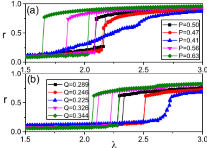
Together with , Zhang et al. also introduced the quantity
| (111) |
where . The quantity measures the average connection between nodes with large and small , and repeating the exchanging process driven by Eq. (70), it is possible to decrease or increase . Figure 77(b) shows the resulting synchronization transitions at different values of . Similarly to Fig. 77(a), the progressive decreasing of has the effect of eventually leading to a second-order transition.
In some circumstances, however, the natural frequencies of the oscillators are also not changeable. To overcome this limitation, Zhang et al. recently presented another efficient method to control ES [438]. The idea is to introduce a small fraction of contrarians to suppress the growing of larger clusters, in contrast to the conformists. There are two approaches to define a conformist or a contrarian. In the first method, a contrarian oscillator will receive interactions from its neighbors via a negative coupling strength, while a conformist oscillator will receive interactions from its neighbors via a positive coupling strength [391, 439]. The model is as follows
| (112) |
where the conformists have positive while the contrarians have negative . For simplicity, the coupling strength is set at the same amplitude with for all conformists and for all contrarians.
In the second method, a contrarian oscillator gives negative coupling to each of its neighbors, while a conformist oscillator gives a positive coupling to each of its neighbors [387, 440, 441]. The model can be written as follows
| (113) |
where the conformists contribute positive , while the contrarians contribute negative . Once again, all strengths are set at the same amplitude , with for all conformists and for all contrarians.
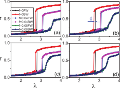
The first case considered is that of random uniformly distributed contrarians, with the definition of contrarian in Eq. (112) (this setting is called the random-case1). Let represents the fraction of contrarians, i.e. the ratio between the number of contrarians and the total number of oscillators. Figure 78(a) shows how the order parameter changes with for and , respectively. It is easy to see that there are hysteretic loops for the cases of and , but no loop is present for the case of , indicating that the first-order transition to synchronization has been changed into a second-order transition. A similar scenario, reported in Fig. 78(b), characterizes the case of random uniformly distributed contrarians with the definition of Eq. (113), called the random-case2. In order to inspect how the distribution of contrarians influences the controlling effect, contrarians are heterogeneously distributed in the network. Figure 78(c) (Eq. 78(d)) shows the case of heterogeneously distributed contrarians with the definition given in Eq. (112) (Eq. (113)) called the hetero-case1 (the hetero-case2). Comparing the four panels of Fig. 78, it is clear that in all cases a second-order phase transition is obtained when .
From Fig. 78, it can be also noticed that the transition point increases with the increase of . In this way, the induced second-order transition point will be much larger than the original first-order transition point . This means that not only the first-order transition is suppressed but also the transition point will be postponed, which is a relevant result in real systems with potential cascading risk.
This finding may be also useful in explaining the normal functioning of brain. It is well known that there are both excitatory and inhibitory neurons in cortical neural networks. The excitatory neurons comprise the majority () of the neuronal population, and are largely homogeneous. The inhibitory neurons comprise only of the neuron population, but are extremely heterogeneous, and take the role of controlling and coordinating the activity of large populations of local neurons [442, 443]. One can then imagining, that the excitatory and inhibitory neurons are in fact the conformists and contrarians, respectively, and that the existence of inhibitory neurons in brain network is necessary not only for sustaining its normal behavior, but also for preventing its abnormal functioning.
6 Conclusions and future perspectives
After having revisited the main theory (and some applications) of explosive percolation and synchronization in complex networks, we end this review with a few concluding remarks, that have the aim of spotting problems that still remain open to future progresses, as well as of offering a few thoughtful considerations about what are the questions of relevance that should (in our opinion, hopefully soon) attract the attention of scientists in this area.
Explosive percolation was largely examined in Chapter 2, and its main applications in physical systems discussed in Section 5.1. The process of percolation refers to the emergence of large-scale connectivity on an underlying network, or lattice. The extensive studies of EP only started on 2009, following a seminal work by Achlioptas, where it was pointed out that introducing competitive mechanisms in the selection of bonds to be added to a graph, the threshold of the percolation process can be significantly postponed, and moreover, the giant cluster emerges after a number of steps that is much smaller than the system size. As a consequence, the order parameter exhibits an extremely abrupt jump at the percolation point, which makes this situation drastically different from classical, random, percolation.
As reported in full details in Chapter 2, many other algorithms and models have been introduced and studied from 2009, and so far EP has been intensively investigated on many networks topologies, including 2D lattices, 3D or high-D lattices, Bethe lattices, ER networks, SF networks, modular networks, and real-world networks. All these works have triggered a big debate in the community, aiming at clarifying whether the observed transitions are really discontinuous or not. While the existence of a seemingly discontinuous jump in the order parameter of the original Achlioptas model is universally recognized, careful numerical investigations of the cooperation, phase coexistence, and nucleation (as well as strict theoretical proofs) have demonstrated that EP in that model is actually continuous in the thermodynamic limit, but it belongs to a universality class different from any other previously considered.
Furthermore (and notably), consensus has been found on the fact that some other models of percolation (such as the k-core percolation model, the spanning cluster-avoiding model, the two-species cluster aggregation model, or the models of jamming on low-dimensional lattices) lead to truly discontinuous transitions. Therefore, it is now fully accepted that the term “explosive” has to refer to the unusual feature which distinguishes the critical behavior of Achlioptas processes from both ordinary and truly discontinuous models.
There are issues that we believe still need efforts from the scientific community. One is that, undoubtedly, more theoretical and numerical studies on the scaling properties and critical exponents in EP are in order, to clarify which new features characterize the critical behavior associated to explosive percolation. Another is the need of exploring EP in other realistic situations (real-world systems or experiments), such as, for instance the cascading failure processes in power grids. And finally, the hope is that the gathered knowledge will help devising methods to control EP, i.e. to enhance or suppress it, when necessary or when desired.
On the other side, ES has been largely discussed in Chapter 4, and its main applications described in Section 5.2. From a historical point of view, we saw that the discovery of ES went through a somehow tortuous path: the community was initially apathetic to the early evidences of first order transitions to synchronization in the thermodynamic limit of a model of globally coupled phase oscillators. Such a situation of guilty indifference persisted for long time, up to when it was clarified that a positive correlation between the natural frequencies of oscillators and the degrees of nodes could produce abrupt cooperative behaviors. For the first time, it was realized that a complete understanding of the nature of phase transitions intimately depended on an explicit interaction between the network topology and the characteristic dynamics of oscillators, and therefore much attention has been recently paid to ES, which begot today great progresses, including theoretical understandings and experimental confirmations.
Let us concentrate on a few issues that possibly will become hot topics on ES.
The first is extending the study of explosive transitions to the case of partial and cluster synchronization, a large area of research, indeed, having to do with cases (like brain functioning, or stock market dynamics, to quote just two examples) for which synchronization on the whole system scale is not possible nor desirable, but rather collective arrangements emerge at the system’s micro- and meso-scales. How to realize explosive transitions to these latter states from the incoherent behavior is still an open question.
The second is bridging ES with specific mixed states of coupled oscillators. Recently, indeed, Zhang et al. proposed a bridge between ES and chimera state [444], and found that they can both coexist within the same coupled system. Further studies on the relationship between ES and chimera state are certainly to be expected soon. Furthermore, since it is now understood that ES can be considered as a dynamical percolation process in phase space, an issue of the utmost relevance is clarifying how one can use the results of explosive percolation for a better control of ES. Therefore, further studies on the relationship between ES and explosive percolation are certainly necessary.
It is convenient to spend a few words on the novel, non-stationary, state that has been described in Section 4.4, the Bellerophon state. In globally coupled nonidentical oscillators, this state can indeed emerge, made of quantized clusters where oscillators are neither phase- nor frequency-locked. Oscillators’ instantaneous speeds are different within the clusters, but they are correlated and, more importantly, they behave periodically in time so that their average values are the same. So far, it has been found that the Bellerophon states occur in fact in a pretty wide context of globally coupled oscillators, and for various typical frequency distributions. Physically, such a state can be regarded as a weaker form of coherence achieved by the coupled oscillators when the control parameter is at an intermediate value, or (in other words) as a transitional state between the incoherent and the phase-locked state: on the one hand the control parameter is not strong enough to completely entrain the system into the phase-locked state, on the other hand it is adequately large to maintain certain correlations among the instantaneous frequencies of oscillators.
Certainly, a lot of future work is in order to unveil Bellerophon states in other oscillatory models, as well as to check if (and under which conditions) the hypothesis of a global coupling can be relaxed to that of a complex network architecture. On the other side, we are totally confident that the discovery of Bellerophon states will stimulate the search for a better theoretical description and characterization, as well as a special care in seeking for such novel states in experimental and natural systems.
Finally, another interesting issue is deepening and enhancing the knowledge of ES in physical systems, where the space embedding (and therefore the lengths of physical links, such as synapses in real neural systems or power lines in power grids), or the multiple level character of interactions between the units (which would require a multi-layer network representation) may play a key role. The study of ES in physically embedded and multi-layer networks is still in its infancy, and we firmly believe that it should instead attract soon a lot of attention, due to its evident relevance for practical applications.
Although beyond the scope of this review, it is worth mentioning that other abrupt transitions have been recently described in networked systems, having to do with spreading processes (like epidemics with co-infection [445, 446] or re-infection [447] mechanisms), spontaneous recovery in dynamical networks [448], and social games using the inertial majority-vote model [449].
7 Acknowledgements
We would like to acknowledge gratefully all colleagues with whom we maintained (and are currently maintaining) interactions and discussions on the topics covered in the report.
In particular, we would like to thank A. Amann, R. Amritkar, F.T. Arecchi, A. Arenas, S. Assenza, V. Avalos-Gaytán, V. Beato, E. Ben Jacob, G. Bianconi, B. Blasius, I. Bonamassa, J. Bragard, J.M. Buldú, J. Burguete, T. Carroll, R. Criado, M. Courbage, M. Danziger, A. Díaz-Guilera, A.L. Do, S.N. Dorogovtsev, E. Estrada, J. García-Ojalvo, C. del Genio, S. Gómez, J. Gómez-Gardeñes, C. Grebogi, P. Grigolini, R. Gutiérrez, M. Hassler, S. Havlin, H.G.E. Hentschel, A. Hramov, D-U. Hwang, R. Jaimes-Reátegui, S. Jalan, M. Jusup, A. Koronovskii, J. Kurths, V. Latora, C. Letellier, D. Li, R. Livi, H. Mancini, J.H. Martinez, D. Maza, J.F.F Mendes, R. Meucci, E. Mihaliuk, G. Mindlin, Y. Moreno, O. Moskalenko, A. Navas, M. Newmann, Y. Ofran, S. Olmi, D. Papo, D. Pazó, L.M. Pecora, M. Perc, T. Pereira, A. Pikovski, A.N. Pisarchick, I. Procaccia, T. Qiu, A.A. Rad, M. Romance, M. Rosenblum, R. Roy, D. de Santos-Sierra, J.R. Sevilla Escoboza, K. Showalter, M. Small, S. Solomon, F. Sorrentino, R. Stoop, S. Strogatz, K. Syamal Dana, A. Torcini, V. Tsioutsiou, J.A. Villacorta-Atienza, V. Vlasov, L. Wang, D. Yu, M. Zanin, X. Zhang.
The huge number of inspiring discussions with them (and their sharing with us of unpublished results on the subject) opened up our minds, and are largely responsible for having encouraged us to write this review.
Furthermore, we would like to acknowledge the financial support received by: 1) the Spanish MINECO under projects FIS2012- 38949-C03-01 and FIS2013-41057-P; 2) the NNSF of China under Grant Nos. 11305062, 11135001, 11375066, and 61374169; JA, IL, and ISN acknowledge support from GARECOM, Group of Research Excellence URJC-Banco de Santander.
References
References
- [1] G. Jaeger, The Ehrenfest classification of phase transitions: introduction and evolution, Archive for History of Exact Sciences 53 (1) (1998) 51–81. doi:10.1007/s004070050021. http://dx.doi.org/10.1007/s004070050021
- [2] D. Stauffer, A. Aharony, Introduction to Percolation Theory, Taylor & Francis, 1992. https://books.google.co.uk/books?id=7TlJk_sUsJ0C
- [3] B. Bollobás, O. Riordan, Percolation, Cambridge university press, Cambridge, New York, Melbourne, 2006. http://opac.inria.fr/record=b1120423
- [4] I. Blekhman, Synchronization in Science and Technology, American Society of Mechanical Engineers, 1988.
- [5] S. Boccaletti, J. Kurths, G. Osipov, D. Valladares, C. Zhou, The synchronization of chaotic systems, Phys. Rep. 366 (1–2) (2002) 1 – 101. doi:10.1016/S0370-1573(02)00137-0.
- [6] S. Strogatz, Sync: The emerging science of spontaneous order, Hyperion, 2003.
- [7] S. Boccaletti, The Synchronized Dynamics of Complex Systems, Elsevier, 2008.
- [8] A. Pikovsky, M. Rosenblum, J. Kurths, Synchronization: A Universal Concept in Nonlinear Sciences, Cambridge University Press, 2001.
- [9] D. Achlioptas, R. M. D’Souza, J. Spencer, Explosive percolation in random networks, Science 323 (5920) (2009) 1453–1455. doi:10.1126/science.1167782. http://www.sciencemag.org/content/323/5920/1453.abstract
- [10] Y. S. Cho, B. Kahng, Discontinuous percolation transitions in real physical systems, Phys. Rev. E 84 (2011) 050102. doi:10.1103/PhysRevE.84.050102. http://link.aps.org/doi/10.1103/PhysRevE.84.050102
- [11] R. A. da Costa, S. N. Dorogovtsev, A. V. Goltsev, J. F. F. Mendes, Explosive percolation transition is actually continuous, Phys. Rev. Lett. 105 (2010) 255701. doi:10.1103/PhysRevLett.105.255701. http://link.aps.org/doi/10.1103/PhysRevLett.105.255701
- [12] P. Grassberger, C. Christensen, G. Bizhani, S.-W. Son, M. Paczuski, Explosive percolation is continuous, but with unusual finite size behavior, Phys. Rev. Lett. 106 (2011) 225701. doi:10.1103/PhysRevLett.106.225701. http://link.aps.org/doi/10.1103/PhysRevLett.106.225701
- [13] O. Riordan, L. Warnke, Explosive percolation is continuous, Science 333 (6040) (2011) 322–324. doi:10.1126/science.1206241. http://www.sciencemag.org/cgi/doi/10.1126/science.1206241
- [14] D. Pazó, Thermodynamic limit of the first-order phase transition in the Kuramoto model, Phys. Rev. E 72 (4) (2005) 046211. doi:10.1103/PhysRevE.72.046211. http://journals.aps.org/pre/abstract/10.1103/PhysRevE.72.046211http://link.aps.org/doi/10.1103/PhysRevE.72.046211
- [15] J. Gómez-Gardeñes, S. Gómez, A. Arenas, Y. Moreno, Explosive synchronization transitions in scale-free networks, Phys. Rev. Lett. 106 (12) (2011) 1–4. doi:10.1103/PhysRevLett.106.128701. http://link.aps.org/doi/10.1103/PhysRevLett.106.128701
- [16] I. Leyva, R. Sevilla-Escoboza, J. M. Buldú, I. Sendiña-Nadal, J. Gómez-Gardeñes, A. Arenas, Y. Moreno, S. Gómez, R. Jaimes-Reátegui, S. Boccaletti, Explosive first-order transition to synchrony in networked chaotic oscillators, Phys. Rev. Lett. 108 (2012) 168702. doi:10.1103/PhysRevLett.108.168702. http://link.aps.org/doi/10.1103/PhysRevLett.108.168702
- [17] I. Leyva, A. Navas, I. Sendiña-Nadal, J. A. Almendral, J. M. Buldú, M. Zanin, D. Papo, S. Boccaletti, Explosive transitions to synchronization in networks of phase oscillators, Sci. Rep. 3 (2013) 1281. doi:10.1038/srep01281. http://www.pubmedcentral.nih.gov/articlerender.fcgi?artid=3573336{&}tool=pmcentrez{&}rendertype=abstracthttp://www.nature.com/doifinder/10.1038/srep01281
- [18] I. Leyva, I. Sendiña-Nadal, J. A. Almendral, A. Navas, S. Olmi, S. Boccaletti, Explosive synchronization in weighted complex networks, Phys. Rev. E 88 (4) (2013) 042808. doi:10.1103/PhysRevE.88.042808. http://link.aps.org/doi/10.1103/PhysRevE.88.042808http://journals.aps.org/pre/abstract/10.1103/PhysRevE.88.042808
- [19] X. Zhang, Y. Zou, S. Boccaletti, Z. Liu, Explosive synchronization as a process of explosive percolation in dynamical phase space, Sci. Rep. 4 (2014) 5200. doi:10.1038/srep05200. http://www.ncbi.nlm.nih.gov/pubmed/24903808http://www.nature.com/doifinder/10.1038/srep05200
- [20] Y. Zou, T. Pereira, M. Small, Z. Liu, J. Kurths, Basin of attraction determines hysteresis in explosive synchronization, Phys. Rev. Lett. 112 (11) (2014) 114102. doi:10.1103/PhysRevLett.112.114102. http://link.aps.org/doi/10.1103/PhysRevLett.112.114102http://journals.aps.org/prl/abstract/10.1103/PhysRevLett.112.114102
- [21] X. Zhang, S. Boccaletti, S. Guan, Z. Liu, Explosive synchronization in adaptive and multilayer networks, Phys. Rev. Lett. 114 (3) (2015) 038701. doi:10.1103/PhysRevLett.114.038701. http://link.aps.org/doi/10.1103/PhysRevLett.114.038701
- [22] I. Sendiña-Nadal, I. Leyva, A. Navas, J. A. Villacorta-Atienza, J. A. Almendral, Z. Wang, S. Boccaletti, Effects of degree correlations on the explosive synchronization of scale-free networks, Phys. Rev. E 91 (3) (2015) 032811. doi:10.1103/PhysRevE.91.032811. http://link.aps.org/doi/10.1103/PhysRevE.91.032811
- [23] Y. Kuramoto, Chemical Oscillations, Waves, and Turbulence, Springer-Verlag, 1984. doi:10.1007/978-3-642-69689-3.
- [24] N. Araújo, P. Grassberger, B. Kahng, K. Schrenk, R. Ziff, Recent advances and open challenges in percolation, Eur. Phys. J. Spec. Top. 223 (11) (2014) 2307–2321. doi:10.1140/epjst/e2014-02266-y. http://link.springer.com/10.1140/epjst/e2014-02266-y
- [25] N. Bastas, P. Giazitzidis, M. Maragakis, K. Kosmidis, Explosive percolation: Unusual transitions of a simple model, Physica A: Statistical Mechanics and its Applications 407 (2014) 54–65. doi:10.1016/j.physa.2014.03.085.
- [26] A. A. Saberi, Recent advances in percolation theory and its applications, Rep. 578 (2015) 1–32. doi:10.1016/j.physrep.2015.03.003.
- [27] R. M. D’Souza, J. Nagler, Anomalous critical and supercritical phenomena in explosive percolation, Nat. Phys. 11 (2015) 531–538. doi:10.1038/NPHYS3378.
- [28] J. Adler, Bootstrap percolation, Physica A 453 (1991) 171. doi:10.1016/0378-4371(91)90295-N.
- [29] E. A. Holroyd, Sharp metastability threshold for two-dimensional bootstrap percolation, Probability Theory and Related Fields 125 (2) (2003) 195–224. doi:10.1007/s00440-002-0239-x. http://dx.doi.org/10.1007/s00440-002-0239-x
- [30] J. Chalupa, P. L. Leath, G. R. Reich, Bootstrap percolation on a bethe lattice, Journal of Physics C: Solid State Physics 12 (1) (1979) L31. http://stacks.iop.org/0022-3719/12/i=1/a=008
- [31] S. N. Dorogovtsev, A. V. Goltsev, J. F. F. Mendes, k-core organization of complex networks, Phys. Rev. Lett. 96 (2006) 040601. doi:10.1103/PhysRevLett.96.040601.
- [32] P. Echenique, J. Gómez-Gardeñes, Y. Moreno, Dynamics of jamming transitions in complex networks, EPL (Europhysics Letters) 71 (2) (2005) 325–331. doi:10.1209/epl/i2005-10080-8. http://iopscience.iop.org/0295-5075/71/2/325http://stacks.iop.org/0295-5075/71/i=2/a=325?key=crossref.f7b66b9054b97e7a2a161cb5bca351f8
- [33] R. M. Ziff, Explosive growth in biased dynamic percolation on two-dimensional regular lattice networks, Phys. Rev. Lett. 103 (2009) 045701. doi:10.1103/PhysRevLett.103.045701.
- [34] F. Radicchi, S. Fortunato, Explosive percolation: A numerical analysis, Phys. Rev. E 81 (2010) 036110. doi:10.1103/PhysRevE.81.036110. http://link.aps.org/doi/10.1103/PhysRevE.81.036110
- [35] R. M. Ziff, Scaling behavior of explosive percolation on the square lattice, Phys. Rev. E 82 (2010) 051105. doi:10.1103/PhysRevE.82.051105.
- [36] N. Bastas, K. Kosmidis, P. Argyrakis, Explosive site percolation and finite-size hysteresis, Phys. Rev. E 84 (2011) 066112. doi:10.1103/PhysRevE.84.066112.
- [37] W. Choi, S.-H. Yook, Y. Kim, Explosive site percolation with a product rule, Phys. Rev. E 84. doi:10.1103/PhysRevE.84.020102.
- [38] S. Angst, S. R. Dahmen, H. Hinrichsen, A. Hucht, M. P. Magiera, Explosive ising, J. Stat. Mech. 2012 (06) (2012) L06002. doi:10.1088/1742-5468/2012/06/L06002.
- [39] J. Li, M. Östling, Corrected finite-size scaling in percolation, Phys. Rev. E 86 (2012) 040105. doi:10.1103/PhysRevE.86.040105. http://link.aps.org/doi/10.1103/PhysRevE.86.040105
- [40] W. Choi, S.-H. Yook, Y. Kim, Bond-site duality and nature of the explosive-percolation phase transition on a two-dimensional lattice, Phys. Rev. E 86 (2012) 051126. doi:10.1103/PhysRevE.86.051126.
- [41] S. D. S. Reis, A. A. Moreira, J. Andrade, Nonlocal product rules for percolation, Phys. Rev. E 85 (2012) 041112. doi:10.1103/PhysRevE.85.041112.
- [42] W. Choi, H. Chae, S.-H. Yook, Y. Kim, Dimensional dependence of phase transitions in explosive percolation, Phys. Rev. E 90 (2014) 022123. doi:10.1103/PhysRevE.90.022123.
- [43] H. Chae, S.-H. Yook, Y. Kim, Explosive percolation on the bethe lattice, Phys. Rev. E 85 (2012) 051118. doi:10.1103/PhysRevE.85.051118.
- [44] Y. S. Cho, S.-W. Kim, J. D. Noh, B. Kahng, D. Kim, Finite-size scaling theory for explosive percolation transitions, Phys. Rev. E 82 (2010) 042102. doi:10.1103/PhysRevE.82.042102.
- [45] Y. Kim, Y.-k. Yun, S.-H. Yook, Explosive percolation in a nanotube-based system, Phys. Rev. E 82 (2010) 061105. doi:10.1103/PhysRevE.82.061105. http://link.aps.org/doi/10.1103/PhysRevE.82.061105
- [46] J. Nagler, A. Levina, M. Timme, Impact of single links in competitive percolation, Nat. Phys. 7 (2011) 265–270. doi:10.1038/NPHYS1860.
- [47] Y. S. Cho, B. Kahng, Suppression effect on explosive percolation, Phys. Rev. Lett. 107 (2011) 275703. doi:10.1103/PhysRevLett.107.275703. http://link.aps.org/doi/10.1103/PhysRevLett.107.275703
- [48] Y. S. Cho, J. S. Kim, J. Park, B. Kahng, D. Kim, Percolation transitions in scale-free networks under the achlioptas process, Phys. Rev. Lett. 103 (1357) (2009) 02. doi:10.1103/PhysRevLett.103.135702.
- [49] F. Radicchi, S. Fortunato, Explosive Percolation in Scale-Free Networks, Phys. Rev. Lett. 103 (16) (2009) 168701. doi:10.1103/PhysRevLett.103.168701. http://link.aps.org/doi/10.1103/PhysRevLett.103.168701
- [50] H. D. Rozenfeld, L. K. Gallos, H. A. Makse, Explosive percolation in the human protein homology network, Eur. Phys. J. B 75 (2010) 305–310. doi:10.1140/epjb/e2010-00156-8.
- [51] S. Squires, K. Sytwu, D. Alcala, T. M. Antonsen, E. Ott, M. Girvan, Weakly explosive percolation in directed networks, Phys. Rev. E 87 (2013) 052127. doi:10.1103/PhysRevE.87.052127. http://link.aps.org/doi/10.1103/PhysRevE.87.052127
- [52] E. J. Friedman, A. S. Landsberg, Construction and analysis of random networks with explosive percolation, Phys. Rev. Lett. 103 (2009) 255701. doi:10.1103/PhysRevLett.103.255701. http://link.aps.org/doi/10.1103/PhysRevLett.103.255701
- [53] N. A. M. Araújo, S. Andrade, R. M. Ziff, H. J. Herrmann, Tricritical point in explosive percolation, Phys. Rev. Lett. 106 (2011) 095703. doi:10.1103/PhysRevLett.106.095703.
- [54] J. S. Andrade, H. J. Herrmann, A. A. Moreira, C. L. N. Oliveira, Transport on exploding percolation clusters, Phys. Rev. E 83 (2011) 031133. doi:10.1103/PhysRevE.83.031133.
- [55] P. Giazitzidis, P. Argyrakis, Generalized achlioptas process for the delay of criticality in the percolation process, Phys. Rev. E 88 (2013) 024801. doi:10.1103/PhysRevE.88.024801.
- [56] H. Hooyberghs, B. V. Schaeybroeck, Criterion for explosive percolation transitions on complex networks, Phys. Rev. E 83 (2011) 032101. doi:10.1103/PhysRevE.83.032101.
- [57] J. H. Qian, D. D. Han, Y. G. Ma, Criticality and continuity of explosive site percolation in random networks, EPL (Europhysics Letters) 100 (4) (2012) 48006. doi:10.1209/0295-5075/100/48006. http://stacks.iop.org/0295-5075/100/i=4/a=48006
- [58] R. K. Pan, M. Kivelä, J. Saramäki, K. Kaski, J. Kertész, Using explosive percolation in analysis of real-world networks, Phys. Rev. E 83 (2011) 046112. doi:10.1103/PhysRevE.83.046112.
- [59] J. Nagler, T. Tiessen, H. W. Gutch, Continuous percolation with discontinuities, Phys. Rev. X 2 (2012) 031009. doi:10.1103/PhysRevX.2.031009.
- [60] O. Riordan, L. Warnke, Achlioptas processes are not always self-averaging, Phys. Rev. E 86 (2012) 011129. doi:10.1103/PhysRevE.86.011129.
- [61] X. Zhang, X. Hu, J. Kurths, Z. Liu, Explosive synchronization in a general complex network, Phys. Rev. E 88 (1) (2013) 010802. doi:10.1103/PhysRevE.88.010802. http://link.aps.org/doi/10.1103/PhysRevE.88.010802
- [62] R. M. D’Souza, M. Mitzenmacher, Local cluster aggregation models of explosive percolation, Phys. Rev. Lett. 104 (2010) 195702. doi:10.1103/PhysRevLett.104.195702. http://link.aps.org/doi/10.1103/PhysRevLett.104.195702
- [63] H. Chen, G. He, F. Huang, C. Shen, Z. Hou, Explosive synchronization transitions in complex neural networks, Chaos 23 (3) (2013) 033124. doi:10.1063/1.4818543.
- [64] R. A. da Costa, S. N. Dorogovtsev, A. V. Goltsev, J. F. F. Mendes, Critical exponents of the explosive percolation transition, Phys. Rev. E 89 (2014) 042148. doi:10.1103/PhysRevE.89.042148.
- [65] R. A. da Costa, S. N. Dorogovtsev, A. V. Goltsev, J. F. F. Mendes, Solution of the explosive percolation quest: Scaling functions and critical exponents, Phys. Rev. E 90 (2014) 022145. doi:10.1103/PhysRevE.90.022145.
- [66] R. A. da Costa, S. N. Dorogovtsev, A. V. Goltsev, J. F. F. Mendes, Solution of the explosive percolation quest, II. Infinite-order transition produced by the initial distributions of clusters, Phys. Rev. E 91 (2015) 032140. doi:10.1103/PhysRevE.91.032140.
- [67] R. A. da Costa, S. N. Dorogovtsev, A. V. Goltsev, J. F. F. Mendes, Inverting the achlioptas rule for explosive percolation, Phys. Rev. E 91 (2015) 042130. doi:10.1103/PhysRevE.91.042130.
- [68] S. D. Yi, W. S. Jo, B. J. Kim, S.-W. Son, Percolation properties of growing networks under an achlioptas process, EPL (Europhysics Letters) 103 (2) (2013) 26004. http://stacks.iop.org/0295-5075/103/i=2/a=26004
- [69] W. Chen, X. Cheng, Z. Zheng, N. N. Chung, R. M. D’Souza, J. Nagler, Unstable supercritical discontinuous percolation transitions, Phys. Rev. E 88 (2013) 042152. doi:10.1103/PhysRevE.88.042152. http://link.aps.org/doi/10.1103/PhysRevE.88.042152
- [70] W. Chen, R. M. D’Souza, Explosive percolation with multiple giant components, Phys. Rev. Lett. 106 (2011) 115701. doi:10.1103/PhysRevLett.106.115701. http://link.aps.org/doi/10.1103/PhysRevLett.106.115701
- [71] K. J. Schrenk, A. Felder, S. Deflorin, N. A. M. Araújo, R. M. D’Souza, H. J. Herrmann, Bohman-frieze-wormald model on the lattice, yielding a discontinuous percolation transition, Phys. Rev. E 85 (2012) 031103. doi:10.1103/PhysRevE.85.031103. http://link.aps.org/doi/10.1103/PhysRevE.85.031103
- [72] Y. Zhang, W. Wei, B. Guo, R. Zhang, Z. Zheng, Formation mechanism and size features of multiple giant clusters in generic percolation processes, Phys. Rev. E 86 (2012) 051103. doi:10.1103/PhysRevE.86.051103.
- [73] W. Chen, Z. Zheng, R. M. D’Souza, Deriving an underlying mechanism for discontinuous percolation, EPL (Europhysics Letters) 100 (6) (2012) 66006. doi:10.1209/0295-5075/100/66006.
- [74] W. Chen, M. Schröder, R. M. D’Souza, D. Sornette, J. Nagler, Microtransition cascades to percolation, Phys. Rev. Lett. 112 (2014) 155701. doi:10.1103/PhysRevLett.112.155701. http://link.aps.org/doi/10.1103/PhysRevLett.112.155701
- [75] A. Waagen, R. M. D’Souza, Given enough choice, simple local rules percolate discontinuously, Eur. Phys. J. B 87 (12) (2014) 1–10. doi:10.1140/epjb/e2014-50278-x.
- [76] Y. Chen, Z. Cao, S. Wang, G. Hu, Self-organized correlations lead to explosive synchronization, Phys. Rev. E 91 (2) (2015) 022810. doi:10.1103/PhysRevE.91.022810. http://journals.aps.org/pre/abstract/10.1103/PhysRevE.91.022810http://link.aps.org/doi/10.1103/PhysRevE.91.022810
- [77] A. A. Moreira, E. A. Oliveira, S. D. S. Reis, H. J. Herrmann, J. S. Andrade, Hamiltonian approach for explosive percolation, Phys. Rev. E 81 (2010) 040101. doi:10.1103/PhysRevE.81.040101. http://link.aps.org/doi/10.1103/PhysRevE.81.040101
- [78] N. A. M. Araújo, H. J. Herrmann, Explosive percolation via control of the largest cluster, Phys. Rev. Lett. 105 (2010) 035701. doi:10.1103/PhysRevLett.105.035701.
- [79] Y. S. Cho, B. Kahng, D. Kim, Cluster aggregation model for discontinuous percolation transitions, Phys. Rev. E 81 (2010) 030103(R). doi:10.1103/PhysRevE.81.030103.
- [80] S. S. Manna, A. Chatterjee, A new route to explosive percolation, Physica A 390 (2011) 177–182. doi:10.1016/j.physa.2010.10.009.
- [81] K. J. Schrenk, N. A. M. Araújo, H. J. Herrmann, Gaussian model of explosive percolation in three and higher dimensions, Phys. Rev. E 84 (2011) 041136. doi:10.1103/PhysRevE.84.041136.
- [82] N. N. Chung, L. Y. Chew, C. H. Lai, Spectral analysis on explosive percolation, EPL (Europhysics Letters) 101 (6) (2013) 66003. http://stacks.iop.org/0295-5075/101/i=6/a=66003
- [83] L. Cao, J. M. Schwarz, Correlated percolation and tricriticality, Phys. Rev. E 86 (2012) 061131. doi:10.1103/PhysRevE.86.061131.
- [84] J. Fan, M. Liu, L. Li, X. Chen, Continuous percolation phase transitions of random networks under a generalized achlioptas process, Phys. Rev. E 85 (2012) 061110. doi:10.1103/PhysRevE.85.061110.
- [85] Y. S. Cho, Y. W. Kim, B. Kahng, Discontinuous percolation in diffusion-limited cluster aggregation, J. Stat. Mech. 2012 (10) (2012) P10004. doi:10.1088/1742-5468/2012/10/P10004. http://stacks.iop.org/1742-5468/2012/i=10/a=P10004
- [86] Y. S. Cho, S. Hwang, H. J. Herrmann, B. Kahng, Avoiding a spanning cluster in percolation models, Science 339 (2013) 1185–1187. doi:10.1126/science.1230813.
- [87] R. M. Ziff, Getting the jump on explosive percolation, Science 339 (6124) (2013) 1159–1160. doi:10.1126/science.1235032. http://www.sciencemag.org/content/339/6124/1159http://www.sciencemag.org/cgi/doi/10.1126/science.1235032
- [88] Y. S. Cho, B. Kahng, Two types of discontinuous percolation transitions in cluster merging processes, Sci. Rep. 5 (2015) 11905. doi:10.1038/srep11905.
- [89] G. J. Baxter, S. N. Dorogovtsev, A. V. Goltsev, J. F. F. Mendes, Bootstrap percolation on complex networks, Phys. Rev. E 82 (1) (2010) 11103. doi:10.1103/PhysRevE.82.011103.
- [90] Y.-Y. Liu, E. Csóka, H. Zhou, M. Pósfai, Core percolation on complex networks, Phys. Rev. Lett. 109 (2012) 205703. doi:10.1103/PhysRevLett.109.205703. http://link.aps.org/doi/10.1103/PhysRevLett.109.205703
- [91] J.-C. Zhao, Explosive synchronization of complex networks with different chaotic oscillators, Chinese Physics B 22 (6) (2013) 060506. doi:10.1088/1674-1056/22/6/060506. http://stacks.iop.org/1674-1056/22/i=6/a=060506?key=crossref.490ad1d60fb495d841ed0d710e173881http://iopscience.iop.org/1674-1056/22/6/060506http://stacks.iop.org/1674-1056/22/i=6/a=060506
- [92] D. Cellai, A. Lawlor, K. A. Dawson, J. P. Gleeson, Critical phenomena in heterogeneous k-core percolation, Phys. Rev. E 87 (2013) 022134. doi:10.1103/PhysRevE.87.022134.
- [93] R. Parshani, S. V. Buldyrev, S. Havlin, Interdependent networks: Reducing the coupling strength leads to a change from a first to second order percolation transition, Phys. Rev. Lett. 105 (2010) 048701. doi:10.1103/PhysRevLett.105.048701.
- [94] R. Parshani, S. V. Buldyrev, S. Havlin, Critical effect of dependency groups on the function of networks, Proc. Natl. Acad. Sci. 108 (3) (2011) 1007–1010. doi:10.1073/pnas.1008404108.
- [95] J. Gao, S. V. Buldyrev, S. Havlin, H. E. Stanley, Robustness of a network of networks, Phys. Rev. Lett. 107 (2011) 195701. doi:10.1103/PhysRevLett.107.195701.
- [96] S.-W. Son, P. Grassberger, M. Paczuski, Percolation transitions are not always sharpened by making networks interdependent, Phys. Rev. Lett. 107 (2011) 195702. doi:10.1103/PhysRevLett.107.195702. http://link.aps.org/doi/10.1103/PhysRevLett.107.195702
- [97] J. Gao, S. V. Buldyrev, H. E. Stanley, S. Havlin, Networks formed from interdependent networks, Nat. Phys. 8 (2012) 40–48. doi:10.1038/NPHYS2180.
- [98] W. Li, A. Bashan, S. V. Buldyrev, H. E. Stanley, S. Havlin, Cascading failures in interdependent lattice networks: The critical role of the length of dependency links, Phys. Rev. Lett. 108 (2012) 228702. doi:10.1103/PhysRevLett.108.228702. http://link.aps.org/doi/10.1103/PhysRevLett.108.228702
- [99] L. M. Shekhtman, Y. Berezin, M. M. Danziger, S. Havlin, Robustness of a network formed of spatially embedded networks, Phys. Rev. E 90 (2014) 012809. doi:10.1103/PhysRevE.90.012809.
- [100] G. J. Baxter, S. N. Dorogovtsev, A. V. Goltsev, J. F. F. Mendes, Avalanche collapse of interdependent networks, Phys. Rev. Lett. 109 (2012) 248701. doi:10.1103/PhysRevLett.109.248701.
- [101] M. Li, X. Jiang, Y. Ma, X. Shen, Z. Zheng, Effect of mixing parts of modular networks on explosive synchronization, EPL (Europhysics Letters) 104 (5) (2013) 58002. doi:10.1209/0295-5075/104/58002.
- [102] K. Panagiotou, R. Spöel, A. Steger, H. Thomas, Explosive percolation in erdös-rényi-like random graph processes, Electron. Notes Discrete Math. 38 (2011) 699–704. doi:10.1016/j.endm.2011.10.017.
- [103] S. Boettcher, V. Singh, R. M. Ziff, Ordinary percolation with discontinuous transitions, Nat. Commun. 3 (2012) 787. doi:10.1038/ncomms1774.
- [104] T. Matsoukas, Abrupt percolation in small equilibrated networks, Phys. Rev. E 91 (2015) 052105. doi:10.1103/PhysRevE.91.052105.
- [105] M. Maksymenko, R. Moessner, K. Shtengel, Reversible first-order transition in pauli percolation, Phys. Rev. E 91 (2015) 062103. doi:10.1103/PhysRevE.91.062103.
- [106] S. V. Buldyrev, R. Parshani, G. Paul, H. E. Stanley, S. Havlin, Catastrophic cascade of failures in interdependent networks, Nature 464 (2010) 1025–1028. doi:10.1038/nature08932.
- [107] H. K. Lee, B. J. Kim, H. Park, Continuity of the explosive percolation transition, Phys. Rev. E 84. doi:10.1103/PhysRevE.84.020101.
- [108] J. Spencer, N. Wormald, Birth control for giants, Combinatorica 27 (2007) 587–628. doi:10.1007/s00493-007-2163-2.
- [109] O. Riordan, L. Warnke, Achlioptas process phase transitions are continuous, Ann. Appl. Probab. 22 (4) (2012) 1450–1464. doi:10.1214/11-AAP798. http://dx.doi.org/10.1214/11-AAP798
- [110] T. Bohman, A. Frieze, N. C. Wormald, Avoidance of a giant component in half the edge set of a random graph, Random Structures & Algorithms 25 (4) (2004) 432–449. doi:10.1002/rsa.20038. http://dx.doi.org/10.1002/rsa.20038
- [111] B. Pittel, J. Spencer, N. C. Wormald, Sudden emergence of a giantk-core in a random graph, J. Comb. Theory B 111 (1996) 67. doi:10.1006/jctb.1996.0036.
- [112] J. M. Schwarz, A. J. Liu, L. Q. Chayes, The onset of jamming as the sudden emergence of an infinite k -core cluster, EPL (Europhysics Letters) 73 (4) (2006) 560. doi:10.1209/epl/i2005-10421-7. http://stacks.iop.org/0295-5075/73/i=4/a=560
- [113] C. L. N. Oliveira, N. A. Araújo, J. S. Andrade, H. J. Herrmann, Explosive electric breakdown due to conducting-particle deposition on an insulating substrate, Phys. Rev. Lett. 113 (2014) 155701. doi:10.1103/PhysRevLett.113.155701.
- [114] D. Landau, K. Binder, A Guide to Monte Carlo Simulations in Statistical Physics, Cambridge University Press, Cambridge, England, 2015. doi:10.1017/CBO9780511614460.
- [115] P. M. Chaikin, T. C. Lubensky, Principles of Condensed Matter Physics, Cambridge University Press, Cambridge, England, 1995. doi:10.1017/CBO9780511813467.
- [116] T. Gross, C. J. D. D’Lima, B. Blasius, Epidemic dynamics on an adaptive network, Phys. Rev. Lett. 96 (2006) 208701. doi:10.1103/PhysRevLett.96.208701. http://link.aps.org/doi/10.1103/PhysRevLett.96.208701
- [117] Y. Zhang, W. Wei, B. Guo, R. Zhang, Z. Zheng, Criticality and scaling behavior of percolation with multiple giant clusters under an achlioptas process, Phys. Rev. E 88 (2013) 062103. doi:10.1103/PhysRevE.88.062103. http://link.aps.org/doi/10.1103/PhysRevE.88.062103
- [118] W. Chen, Z. Zheng, X. Jiang, R. M. D. Souza, Multiple discontinuous percolation transitions on scale-free networks, J. Stat. Mech. (2015) P04011doi:10.1088/1742-5468/2015/04/P04011. http://dx.doi.org/10.1088/1742-5468/2015/04/P04011
- [119] A. D. Bruce, N. B. Wilding, Scaling fields and universality of the liquid-gas critical point, Phys. Rev. Lett. 68 (1992) 193–196. doi:10.1103/PhysRevLett.68.193. http://link.aps.org/doi/10.1103/PhysRevLett.68.193
- [120] V. Privman, Finite-size Scaling Theory. Finite Size Scaling and Numerical Simulation of Statistical Systems, World Scientific, 2014. doi:10.1142/9789814503419_0001.
- [121] L. Tian, D. N. Shi, The nature of explosive percolation phase transition, Physics Letters A 376 (4) (2012) 286–289. doi:10.1016/j.physleta.2011.11.039. http://dx.doi.org/10.1016/j.physleta.2011.11.039
- [122] P. Bergé, Y. Pomeau, C. Vidal, Order Within Chaos: Towards a Deterministic Approach to Turbulence, Wiley, 1985.
- [123] S. Manrubia, A. Mikhailov, D. Zanette, Emergence of dynamical order: synchronization phenomena in complex systems, World Scientific, 2004.
- [124] C. Letellier, L. A. Aguirre, Interplay between synchronization, observability, and dynamics, Phys. Rev. E 82 (1) (2010) 1–11. doi:10.1103/PhysRevE.82.016204.
- [125] E. Bianco-Martinez, M. S. Baptista, C. Letellier, Symbolic computations of nonlinear observability, Phys. Rev. E 91 (6) (2015) 062912. doi:10.1103/PhysRevE.91.062912.
- [126] I. Sendiña-Nadal, C. Letellier, S. Boccaletti, Observability coefficients for predicting the class of synchronizability from the algebraic structure of the local oscillators, Phys. Rev. E xx (x) (2016) xxxxx.
- [127] H. Daido, Intrinsic fluctuations and a phase transition in a class of large populations of interacting oscillators, J. Stat. Phys. 60 (5) (1990) 753–800. doi:10.1007/BF01025993. http://dx.doi.org/10.1007/BF01025993
- [128] A. T. Winfree, Biological rhythms and the behavior of populations of coupled oscillators., Journal of Theoretical Biology 16 (1) (1967) 15–42. doi:10.1016/0022-5193(67)90051-3.
- [129] M. Valdeolmillos, a. Gomis, J. V. Sánchez-Andrés, In vivo synchronous membrane potential oscillations in mouse pancreatic beta-cells: lack of co-ordination between islets, The Journal of Physiology 493 (1) (1996) 9–18. doi:10.1113/jphysiol.1996.sp021361. http://dx.doi.org/10.1113/jphysiol.1996.sp021361
- [130] K. Wood, C. Van den Broeck, R. Kawai, K. Lindenberg, Continuous and discontinuous phase transitions and partial synchronization in stochastic three-state oscillators, Phys. Rev. E 76 (2007) 041132. doi:10.1103/PhysRevE.76.041132. http://link.aps.org/doi/10.1103/PhysRevE.76.041132
- [131] G. Filatrella, N. F. Pedersen, K. Wiesenfeld, Generalized coupling in the kuramoto model, Phys. Rev. E 75 (2007) 017201. doi:10.1103/PhysRevE.75.017201. http://link.aps.org/doi/10.1103/PhysRevE.75.017201
- [132] H.-A. Tanaka, A. J. Lichtenberg, S. Oishi, First order phase transition resulting from finite inertia in coupled oscillator systems, Phys. Rev. Lett. 78 (11) (1997) 2104–2107. doi:10.1103/PhysRevLett.78.2104. http://link.aps.org/doi/10.1103/PhysRevLett.78.2104
- [133] J. A. Acebrón, L. L. Bonilla, R. Spigler, Synchronization in populations of globally coupled oscillators with inertial effects, Phys. Rev. E 62 (2000) 3437–3454. doi:10.1103/PhysRevE.62.3437. http://link.aps.org/doi/10.1103/PhysRevE.62.3437
- [134] M. Choi, H. Kim, D. Kim, H. Hong, Synchronization in a system of globally coupled oscillators with time delay, Phys. Rev. E 61 (1) (2000) 371–381. doi:10.1103/PhysRevE.61.371.
- [135] F. Giannuzzi, D. Marinazzo, G. Nardulli, M. Pellicoro, S. Stramaglia, Phase diagram of a generalized Winfree model, Phys. Rev. E 75 (5) (2007) 051104. doi:10.1103/PhysRevE.75.051104. http://link.aps.org/doi/10.1103/PhysRevE.75.051104
- [136] M. Rosenblum, A. Pikovsky, Self-Organized Quasiperiodicity in Oscillator Ensembles with Global Nonlinear Coupling, Phys. Rev. Lett. 98 (6) (2007) 064101. doi:10.1103/PhysRevLett.98.064101. http://link.aps.org/doi/10.1103/PhysRevLett.98.064101
- [137] S. Strogatz, Nonlinear Dynamics and Chaos: With Applications to Physics, Biology, Chemistry, and Engineering, Advanced book program, Westview Press, 1994. https://books.google.es/books?id=FIYHiBLWCJMC
- [138] V. S. Afraimovich, N. N. Verichev, M. I. Rabinovich, Stochastic synchronization of oscillation in dissipative systems, Radiophysics and Quantum Electronics 29 (9) (1986) 795–803. doi:10.1007/BF01034476.
- [139] L. M. Pecora, T. L. Carroll, Synchronization in chaotic systems, Phys. Rev. Lett. 64 (1990) 821–824. doi:10.1103/PhysRevLett.64.821. http://link.aps.org/doi/10.1103/PhysRevLett.64.821
- [140] L. M. Pecora, T. L. Carroll, Master stability functions for synchronized coupled systems, Phys. Rev. Lett. 80 (1998) 2109–2112. doi:10.1103/PhysRevLett.80.2109. http://link.aps.org/doi/10.1103/PhysRevLett.80.2109
- [141] V. I. Arnol’d, Small denominators. i. mapping the circle onto itself, Izvestiya Rossiiskoi Akademii Nauk. Seriya Matematicheskaya 25 (1) (1961) 21–86.
- [142] M. G. Rosenblum, A. S. Pikovsky, J. Kurths, Phase synchronization of chaotic oscillators, Phys. Rev. Lett. 76 (11) (1996) 1804–1807. doi:10.1103/PhysRevLett.76.1804.
- [143] M. A. Zaks, E.-H. Park, M. G. Rosenblum, J. Kurths, Alternating locking ratios in imperfect phase synchronization, Phys. Rev. Lett. 82 (1999) 4228–4231. doi:10.1103/PhysRevLett.82.4228. http://link.aps.org/doi/10.1103/PhysRevLett.82.4228
- [144] A. Pujol-Peré, O. Calvo, M. A. Matías, J. Kurths, Experimental study of imperfect phase synchronization in the forced lorenz system, Chaos 13 (1) (2003) 319–326. doi:10.1063/1.1525126. http://scitation.aip.org/content/aip/journal/chaos/13/1/10.1063/1.1525126
- [145] M. Rosenblum, A. Pikovsky, J. Kurths, From Phase to Lag Synchronization in Coupled Chaotic Oscillators, Phys. Rev. Lett. 78 (22) (1997) 4193–4196. doi:10.1103/PhysRevLett.78.4193.
- [146] H. U. Voss, Anticipating chaotic synchronization, Phys. Rev. E 61 (2000) 5115–5119. doi:10.1103/PhysRevE.61.5115. http://link.aps.org/doi/10.1103/PhysRevE.61.5115
- [147] H. U. Voss, Erratum: Anticipating chaotic synchronization [phys. rev. e 61, 5115 (2000)], Phys. Rev. E 64 (2001) 039904. doi:10.1103/PhysRevE.64.039904. http://link.aps.org/doi/10.1103/PhysRevE.64.039904
- [148] T. Heil, I. Fischer, W. Elsässer, J. Mulet, C. R. Mirasso, Chaos synchronization and spontaneous symmetry-breaking in symmetrically delay-coupled semiconductor lasers, Phys. Rev. Lett. 86 (5) (2001) 795–798. doi:10.1103/PhysRevLett.86.795.
- [149] J. K. White, M. Matus, J. V. Moloney, Achronal generalized synchronization in mutually coupled semiconductor lasers, Phys. Rev. E 65 (2002) 036229. doi:10.1103/PhysRevE.65.036229. http://link.aps.org/doi/10.1103/PhysRevE.65.036229
- [150] I. Fischer, R. Vicente, J. M. Buldú, M. Peil, C. R. Mirasso, M. C. Torrent, J. García-Ojalvo, Zero-lag long-range synchronization via dynamical relaying, Phys. Rev. Lett. 97 (2006) 123902. doi:10.1103/PhysRevLett.97.123902. http://link.aps.org/doi/10.1103/PhysRevLett.97.123902
- [151] A. Wagemakers, J. M. Buldú, M. A. F. Sanjuan, Experimental demonstration of bidirectional chaotic communication by means of isochronal synchronization, EPL (Europhysics Letters) 81 (4) (2008) 40005. doi:10.1209/0295-5075/81/40005. http://stacks.iop.org/0295-5075/81/i=4/a=40005
- [152] E. Klein, N. Gross, M. Rosenbluh, W. Kinzel, L. Khaykovich, I. Kanter, Stable isochronal synchronization of mutually coupled chaotic lasers, Phys. Rev. E 73 (2006) 066214. doi:10.1103/PhysRevE.73.066214. http://link.aps.org/doi/10.1103/PhysRevE.73.066214
- [153] M. Peil, L. Larger, I. Fischer, Versatile and robust chaos synchronization phenomena imposed by delayed shared feedback coupling, Phys. Rev. E 76 (2007) 045201. doi:10.1103/PhysRevE.76.045201. http://link.aps.org/doi/10.1103/PhysRevE.76.045201
- [154] J. Tiana-Alsina, K. Hicke, X. Porte, M. C. Soriano, M. C. Torrent, J. Garcia-Ojalvo, I. Fischer, Zero-lag synchronization and bubbling in delay-coupled lasers, Phys. Rev. E 85 (2012) 026209. doi:10.1103/PhysRevE.85.026209. http://link.aps.org/doi/10.1103/PhysRevE.85.026209
- [155] I. G. Da Silva, J. M. Buldú, C. R. Mirasso, J. García-Ojalvo, Synchronization by dynamical relaying in electronic circuit arrays, Chaos 16 (4) (2006) 043113. doi:10.1063/1.2374860.
- [156] B. B. Zhou, R. Roy, Isochronal synchrony and bidirectional communication with delay-coupled nonlinear oscillators, Phys. Rev. E 75 (2007) 026205. doi:10.1103/PhysRevE.75.026205. http://link.aps.org/doi/10.1103/PhysRevE.75.026205
- [157] A. Wagemakers, J. M. Buldú, M. A. F. Sanjuán, Isochronous synchronization in mutually coupled chaotic circuits, Chaos 17 (2) (2007) 023128. doi:10.1063/1.2737820.
- [158] A. Englert, W. Kinzel, Y. Aviad, M. Butkovski, I. Reidler, M. Zigzag, I. Kanter, M. Rosenbluh, Zero lag synchronization of chaotic systems with time delayed couplings, Phys. Rev. Lett. 104 (2010) 114102. doi:10.1103/PhysRevLett.104.114102. http://link.aps.org/doi/10.1103/PhysRevLett.104.114102
- [159] J. G. Wu, Z. M. Wu, G. Q. Xia, T. Deng, X. D. Lin, X. Tang, G. Y. Feng, Isochronous synchronization between chaotic semiconductor lasers over 40-km fiber links, IEEE Photonics Technology Letters 23 (24) (2011) 1854–1856. doi:10.1109/LPT.2011.2170212.
- [160] R. Vicente, C. R. Mirasso, I. Fischer, Simultaneous bidirectional message transmission in a chaos-based communication scheme, Opt. Lett. 32 (4) (2007) 403–405. doi:10.1364/OL.32.000403. http://ol.osa.org/abstract.cfm?URI=ol-32-4-403
- [161] R. Vicente, G. Pipa, I. Fischer, C. R. Mirasso, Zero-lag long range synchronization of neurons is enhanced by dynamical relaying, in: J. M. de Sá, L. A. Alexandre, W. Duch, D. Mandic (Eds.), Artificial Neural Networks, Springer Berlin Heidelberg, Berlin, Heidelberg, 2007, pp. 904–913. doi:10.1007/978-3-540-74690-4_92. http://dx.doi.org/10.1007/978-3-540-74690-4_92
- [162] R. Vicente, L. L. Gollo, C. R. Mirasso, I. Fischer, G. Pipa, Dynamical relaying can yield zero time lag neuronal synchrony despite long conduction delays, Proc. Natl. Acad. Sci. 105 (44) (2008) 17157–17162. doi:10.1073/pnas.0809353105. http://www.pnas.org/content/105/44/17157.shorthttp://www.pnas.org/content/105/44/17157
- [163] Z. G. Esfahani, A. Valizadeh, Zero-lag synchronization despite inhomogeneities in a relay system, PLoS ONE 9 (12) (2014) e112688. doi:10.1371/journal.pone.0112688.
- [164] H. U. Voss, Dynamic long-term anticipation of chaotic states, Phys. Rev. Lett. 87 (2001) 014102. doi:10.1103/PhysRevLett.87.014102. http://link.aps.org/doi/10.1103/PhysRevLett.87.014102
- [165] C. Masoller, D. H. Zanette, Anticipated synchronization in coupled chaotic maps with delays, Physica A: Statistical Mechanics and its Applications 300 (3-4) (2001) 359–366. doi:10.1016/S0378-4371(01)00362-4. http://www.sciencedirect.com/science/article/pii/S0378437101003624
- [166] M. Ciszak, O. Calvo, C. Masoller, C. R. Mirasso, R. Toral, Anticipating the response of excitable systems driven by random forcing, Phys. Rev. Lett. 90 (2003) 204102. doi:10.1103/PhysRevLett.90.204102. http://link.aps.org/doi/10.1103/PhysRevLett.90.204102
- [167] R. Toral, C. Masoller, C. R. Mirasso, M. Ciszak, O. Calvo, Characterization of the anticipated synchronization regime in the coupled fitzhugh-nagumo model for neurons, Physica A 325 (1–2) (2003) 192 – 198. doi:http://dx.doi.org/10.1016/S0378-4371(03)00198-5. http://www.sciencedirect.com/science/article/pii/S0378437103001985
- [168] M. Ciszak, F. Marino, R. Toral, S. Balle, Dynamical mechanism of anticipating synchronization in excitable systems, Phys. Rev. Lett. 93 (2004) 114102. doi:10.1103/PhysRevLett.93.114102. http://link.aps.org/doi/10.1103/PhysRevLett.93.114102
- [169] F. S. Matias, P. V. Carelli, C. R. Mirasso, M. Copelli, Anticipated synchronization in a biologically plausible model of neuronal motifs, Phys. Rev. E 84 (2011) 021922. doi:10.1103/PhysRevE.84.021922. http://link.aps.org/doi/10.1103/PhysRevE.84.021922
- [170] M. Kostur, P. Hänggi, P. Talkner, J. L. Mateos, Anticipated synchronization in coupled inertial ratchets with time-delayed feedback: A numerical study, Phys. Rev. E 72 (2005) 036210. doi:10.1103/PhysRevE.72.036210. http://link.aps.org/doi/10.1103/PhysRevE.72.036210
- [171] M. Ciszak, C. Mayol, C. R. Mirasso, R. Toral, Anticipated synchronization in coupled complex ginzburg-landau systems, Phys. Rev. E 92 (2015) 032911. doi:10.1103/PhysRevE.92.032911. http://link.aps.org/doi/10.1103/PhysRevE.92.032911
- [172] H. U. Voss, Real-time anticipation of chaotic states of an electronic circuit, Int. J. Bifurcation Chaos 12 (07) (2002) 1619–1625. doi:10.1142/S0218127402005340.
- [173] S. D. Pethel, N. J. Corron, Q. R. Underwood, K. Myneni, Information flow in chaos synchronization: Fundamental tradeoffs in precision, delay, and anticipation, Phys. Rev. Lett. 90 (2003) 254101. doi:10.1103/PhysRevLett.90.254101. http://link.aps.org/doi/10.1103/PhysRevLett.90.254101
- [174] J. Zamora-Munt, C. R. Mirasso, R. Toral, Suppression of deterministic and stochastic extreme desynchronization events using anticipated synchronization, Phys. Rev. E 89 (2014) 012921. doi:10.1103/PhysRevE.89.012921. http://link.aps.org/doi/10.1103/PhysRevE.89.012921
- [175] S. Sivaprakasam, E. M. Shahverdiev, P. S. Spencer, K. A. Shore, Experimental demonstration of anticipating synchronization in chaotic semiconductor lasers with optical feedback, Phys. Rev. Lett. 87 (2001) 154101. doi:10.1103/PhysRevLett.87.154101. http://link.aps.org/doi/10.1103/PhysRevLett.87.154101
- [176] J. M. Buldú, R. Vicente, T. Pérez, C. R. Mirasso, M. C. Torrent, J. García-Ojalvo, Periodic entrainment of power dropouts in mutually coupled semiconductor lasers, Applied Physics Letters 81 (27) (2002) 5105–5107. doi:10.1063/1.1533837.
- [177] M. Ciszak, C. R. Mirasso, R. Toral, O. Calvo, Predict-prevent control method for perturbed excitable systems, Phys. Rev. E 79 (2009) 046203. doi:10.1103/PhysRevE.79.046203. http://link.aps.org/doi/10.1103/PhysRevE.79.046203
- [178] N. F. Rulkov, M. M. Sushchik, L. S. Tsimring, H. D. I. Abarbanel, Generalized synchronization of chaos in directionally coupled chaotic systems, Phys. Rev. E 51 (2) (1995) 980–994. doi:10.1103/PhysRevE.51.980.
- [179] L. Kocarev, U. Parlitz, Generalized Synchronization, Predictability, and Equivalence of Unidirectionally Coupled Dynamical Systems, Phys. Rev. Lett. 76 (11) (1996) 1816–1819. doi:10.1103/PhysRevLett.76.1816. http://link.aps.org/doi/10.1103/PhysRevLett.76.1816
- [180] K. Pyragas, Weak and strong synchronization of chaos, Phys. Rev. E 54 (5) (1996) R4508–R4511. doi:10.1103/PhysRevE.54.R4508.
- [181] H. D. I. Abarbanel, N. Rulkov, M. Sushchik, Generalized synchronization of chaos: The auxiliary system approach, Phys. Rev. E 53 (5) (1996) 4528–4535. doi:10.1103/PhysRevE.53.4528.
- [182] A. S. Landsman, I. B. Schwartz, Complete chaotic synchronization in mutually coupled time-delay systems, Phys. Rev. E 75 (2) (2007) 026201. doi:10.1103/PhysRevE.75.026201. http://link.aps.org/doi/10.1103/PhysRevE.75.026201
- [183] O. I. Moskalenko, A. A. Koronovskii, A. E. Hramov, S. Boccaletti, Generalized synchronization in mutually coupled oscillators and complex networks, Phys. Rev. E 86 (2012) 036216. doi:10.1103/PhysRevE.86.036216. http://link.aps.org/doi/10.1103/PhysRevE.86.036216
- [184] R. Gutiérrez, R. Sevilla-Escoboza, P. Piedrahita, C. Finke, U. Feudel, J. M. Buldú, G. Huerta-Cuellar, R. Jaimes-Reátegui, Y. Moreno, S. Boccaletti, Generalized synchronization in relay systems with instantaneous coupling, Phys. Rev. E 88 (2013) 052908. doi:10.1103/PhysRevE.88.052908. http://link.aps.org/doi/10.1103/PhysRevE.88.052908
- [185] G. Saxena, A. Prasad, R. Ramaswamy, Amplitude death: The emergence of stationarity in coupled nonlinear systems, Phys. Rep. 521 (5) (2012) 205 – 228, amplitude Death: The Emergence of Stationarity in Coupled Nonlinear Systems. doi:10.1016/j.physrep.2012.09.003. http://www.sciencedirect.com/science/article/pii/S0370157312002645
- [186] A. Koseska, E. Volkov, J. Kurths, Oscillation quenching mechanisms: Amplitude vs. oscillation death, Phys. Rep. 531 (4) (2013) 173–199. doi:10.1016/j.physrep.2013.06.001. http://dx.doi.org/10.1016/j.physrep.2013.06.001
- [187] Y. Kuramoto, Self-entrainment of a population of coupled non-linear oscillators, in: International Symposium on Mathematical Problems in Theoretical Physics, Springer, Berlin, Heidelberg, 1975, pp. 420–422. doi:10.1007/BFb0013365. http://dx.doi.org/10.1007/BFb0013365
- [188] A. T. Winfree, The Geometry of Biological Time, Springer, Berlin, 1980. doi:10.1007/978-1-4757-3484-3.
- [189] J. D. Murray, Mathematical Biology, Springer, Berlin, 1989. doi:10.1007/b98868.
- [190] R. Kapral, K. Showalter (Eds.), Chemical Waves and Patterns, Springer Netherlands, 1995. doi:10.1007/978-94-011-1156-0.
- [191] O.-U. Kheowan, E. Mihaliuk, B. Blasius, I. Sendiña-Nadal, K. Showalter, Wave mediated synchronization of nonuniform oscillatory media, Phys. Rev. Lett. 98 (2007) 074101. doi:10.1103/PhysRevLett.98.074101. http://link.aps.org/doi/10.1103/PhysRevLett.98.074101
- [192] I. Leyva, A. Navas, I. Sendiña-Nadal, J. M. Buldú, J. A. Almendral, S. Boccaletti, Synchronization waves in geometric networks, Phys. Rev. E 84 (2011) 065101. doi:10.1103/PhysRevE.84.065101. http://link.aps.org/doi/10.1103/PhysRevE.84.065101
- [193] G. V. Osipov, J. Kurths, C. Zhou, Synchronization in Oscillatory Networks, Springer Berlin Heidelberg, Berlin, Heidelberg, 2007. doi:10.1007/978-3-540-71269-5_5. http://dx.doi.org/10.1007/978-3-540-71269-5_5
- [194] K. Kaneko, Spatiotemporal Intermittency in Coupled Map Lattices, Prog. Theor. Phys. 74 (5) (1985) 1033–1044. doi:10.1143/PTP.74.1033. http://ptp.oxfordjournals.org/cgi/doi/10.1143/PTP.74.1033
- [195] K. Kaneko, Theory and Applications of Coupled Map Lattices, Wiley, 1993.
- [196] M. Hasler, Y. Maistrenko, O. Popovych, Simple example of partial synchronization of chaotic systems, Phys. Rev. E 58 (5) (1998) 6843–6846. doi:10.1103/PhysRevE.58.6843. http://link.aps.org/doi/10.1103/PhysRevE.58.6843
- [197] J. F. Heagy, T. L. Carroll, L. M. Pecora, Synchronous chaos in coupled oscillator systems, Phys. Rev. E 50 (3) (1994) 1874–1885. doi:10.1103/PhysRevE.50.1874. http://link.aps.org/doi/10.1103/PhysRevE.50.1874
- [198] J. F. Heagy, L. M. Pecora, T. L. Carroll, Short Wavelength Bifurcations and Size Instabilities in Coupled Oscillator Systems, Phys. Rev. Lett. 74 (21) (1995) 4185–4188. doi:10.1103/PhysRevLett.74.4185. http://link.aps.org/doi/10.1103/PhysRevLett.74.4185
- [199] V. N. Belykh, I. V. Belykh, M. Hasler, Hierarchy and stability of partially synchronous oscillations of diffusively coupled dynamical systems, Phys. Rev. E 62 (5) (2000) 6332–6345. doi:10.1103/PhysRevE.62.6332. http://link.aps.org/doi/10.1103/PhysRevE.62.6332
- [200] V. N. Belykh, I. V. Belykh, E. Mosekilde, Cluster synchronization modes in an ensemble of coupled chaotic oscillators, Phys. Rev. E 63 (3) (2001) 036216. doi:10.1103/PhysRevE.63.036216. http://link.aps.org/doi/10.1103/PhysRevE.63.036216
- [201] M. C. Cross, P. C. Hohenberg, Pattern formation outside of equilibrium, Rev. Mod. Phys. 65 (3) (1993) 851–1112. doi:10.1103/RevModPhys.65.851. http://link.aps.org/doi/10.1103/RevModPhys.65.851
- [202] I. S. Aranson, L. Kramer, The world of the complex Ginzburg-Landau equation, Rev. Mod. Phys. 74 (1) (2002) 99–143. doi:10.1103/RevModPhys.74.99. http://link.aps.org/doi/10.1103/RevModPhys.74.99
- [203] K. Kaneko, Globally coupled circle maps, Physica D 54 (1-2) (1991) 5–19. doi:10.1016/0167-2789(91)90103-G. http://linkinghub.elsevier.com/retrieve/pii/016727899190103G
- [204] S. C. Manrubia, A. S. Mikhailov, Mutual synchronization and clustering in randomly coupled chaotic dynamical networks, Phys. Rev. E 60 (2) (1999) 1579–1589. doi:10.1103/PhysRevE.60.1579. http://www.ncbi.nlm.nih.gov/pubmed/11969920http://link.aps.org/doi/10.1103/PhysRevE.60.1579
- [205] O. Popovych, Y. Maistrenko, E. Mosekilde, Loss of coherence in a system of globally coupled maps, Phys. Rev. E 64 (2) (2001) 026205. doi:10.1103/PhysRevE.64.026205. http://link.aps.org/doi/10.1103/PhysRevE.64.026205
- [206] A. Pikovsky, O. Popovych, Y. Maistrenko, Resolving Clusters in Chaotic Ensembles of Globally Coupled Identical Oscillators, Phys. Rev. Lett. 87 (4) (2001) 044102. doi:10.1103/PhysRevLett.87.044102. http://link.aps.org/doi/10.1103/PhysRevLett.87.044102
- [207] L. Kocarev, U. Parlitz, Synchronizing Spatiotemporal Chaos in Coupled Nonlinear Oscillators, Phys. Rev. Lett. 77 (11) (1996) 2206–2209. doi:10.1103/PhysRevLett.77.2206. http://www.ncbi.nlm.nih.gov/pubmed/10061885http://link.aps.org/doi/10.1103/PhysRevLett.77.2206
- [208] D. H. Zanette, A. S. Mikhailov, Condensation in globally coupled populations of chaotic dynamical systems, Phys. Rev. E 57 (1) (1998) 276–281. doi:10.1103/PhysRevE.57.276.
- [209] S. K. Han, C. Kurrer, Y. Kuramoto, Dephasing and bursting in coupled neural oscillators, Phys. Rev. Lett. 75 (17) (1995) 3190–3193. doi:10.1103/PhysRevLett.75.3190. http://link.aps.org/doi/10.1103/PhysRevLett.75.3190
- [210] H. Daido, K. Nakanishi, Diffusion-Induced Inhomogeneity in Globally Coupled Oscillators: Swing-By Mechanism, Phys. Rev. Lett. 96 (5) (2006) 054101. doi:10.1103/PhysRevLett.96.054101. http://link.aps.org/doi/10.1103/PhysRevLett.96.054101
- [211] A. Yeldesbay, A. Pikovsky, M. Rosenblum, Chimeralike States in an Ensemble of Globally Coupled Oscillators, Phys. Rev. Lett. 112 (14) (2014) 144103. doi:10.1103/PhysRevLett.112.144103. http://link.aps.org/doi/10.1103/PhysRevLett.112.144103
- [212] R. E. Mirollo, S. H. Strogatz, Synchronization of Pulse-Coupled Biological Oscillators, SIAM J. Appl. Math. 50 (6) (1990) 1645–1662. doi:10.1137/0150098. http://epubs.siam.org/doi/abs/10.1137/0150098
- [213] C. van Vreeswijk, Partial synchronization in populations of pulse-coupled oscillators, Phys. Rev. E 54 (5) (1996) 5522–5537. doi:10.1103/PhysRevE.54.5522. {<}GotoISI{>}://WOS:A1996VU53700129http://link.aps.org/doi/10.1103/PhysRevE.54.5522
- [214] P. K. Mohanty, A. Politi, A new approach to partial synchronization in globally coupled rotators, J. Phys. A: Math. Gen. 39 (26) (2006) L415–L421. doi:10.1088/0305-4470/39/26/L01. http://stacks.iop.org/0305-4470/39/i=26/a=L01?key=crossref.4dc0349b6e5ac588c039fd291fb5a6cb
- [215] W. Wang, I. Z. Kiss, J. L. Hudson, Experiments on arrays of globally coupled chaotic electrochemical oscillators: Synchronization and clustering, Chaos 10 (1) (2000) 248. doi:10.1063/1.166470. <GotoISI>://000084601400027http://pubs.acs.org/doi/abs/10.1021/jp992471hhttp://scitation.aip.org/content/aip/journal/chaos/10/1/10.1063/1.166470
- [216] L. M. Pecora, Synchronization conditions and desynchronizing patterns in coupled limit-cycle and chaotic systems, Phys. Rev. E 58 (1) (1998) 347–360. doi:10.1103/PhysRevE.58.347. http://link.aps.org/doi/10.1103/PhysRevE.58.347
- [217] D. M. Abrams, S. H. Strogatz, Chimera States for Coupled Oscillators, Phys. Rev. Lett. 93 (17) (2004) 174102. doi:10.1103/PhysRevLett.93.174102. http://link.aps.org/doi/10.1103/PhysRevLett.93.174102
- [218] D. Battogtokh, Y. Kuramoto, Turbulence of nonlocally coupled oscillators in the Benjamin-Feir stable regime, Phys. Rev. E 61 (3) (2000) 3227–3229. doi:10.1103/PhysRevE.61.3227. http://link.aps.org/doi/10.1103/PhysRevE.61.3227
- [219] O. E. Omel’chenko, Y. L. Maistrenko, P. A. Tass, Chimera States: The Natural Link Between Coherence and Incoherence, Phys. Rev. Lett. 100 (4) (2008) 044105. doi:10.1103/PhysRevLett.100.044105. http://link.aps.org/doi/10.1103/PhysRevLett.100.044105
- [220] D. M. Abrams, R. Mirollo, S. H. Strogatz, D. A. Wiley, Solvable Model for Chimera States of Coupled Oscillators, Phys. Rev. Lett. 101 (8) (2008) 084103. doi:10.1103/PhysRevLett.101.084103. http://link.aps.org/doi/10.1103/PhysRevLett.101.084103
- [221] G. Bordyugov, A. Pikovsky, M. Rosenblum, Self-emerging and turbulent chimeras in oscillator chains, Phys. Rev. E 82 (3) (2010) 035205. doi:10.1103/PhysRevE.82.035205. http://link.aps.org/doi/10.1103/PhysRevE.82.035205
- [222] E. A. Martens, C. R. Laing, S. H. Strogatz, Solvable Model of Spiral Wave Chimeras, Phys. Rev. Lett. 104 (4) (2010) 044101. doi:10.1103/PhysRevLett.104.044101. http://link.aps.org/doi/10.1103/PhysRevLett.104.044101
- [223] O. E. Omel’chenko, M. Wolfrum, Y. L. Maistrenko, Chimera states as chaotic spatiotemporal patterns, Phys. Rev. E 81 (6) (2010) 065201. doi:10.1103/PhysRevE.81.065201. http://link.aps.org/doi/10.1103/PhysRevE.81.065201
- [224] I. Omelchenko, Y. Maistrenko, P. Hövel, E. Schöll, Loss of Coherence in Dynamical Networks: Spatial Chaos and Chimera States, Phys. Rev. Lett. 106 (23) (2011) 234102. doi:10.1103/PhysRevLett.106.234102. http://link.aps.org/doi/10.1103/PhysRevLett.106.234102
- [225] M. R. Tinsley, S. Nkomo, K. Showalter, Chimera and phase-cluster states in populations of coupled chemical oscillators, Nat. Phys. 8 (9) (2012) 662–665. doi:10.1038/nphys2371. message:<4F6A52BF.9000105@ds.mpg.de>$\$npapers2://publication/uuid/1D23C05A-616A-4E21-8FF1-412E4F5196BDhttp://www.nature.com/doifinder/10.1038/nphys2371
- [226] S. Nkomo, M. R. Tinsley, K. Showalter, Chimera States in Populations of Nonlocally Coupled Chemical Oscillators, Phys. Rev. Lett. 110 (24) (2013) 244102. doi:10.1103/PhysRevLett.110.244102. http://link.aps.org/doi/10.1103/PhysRevLett.110.244102
- [227] A. M. Hagerstrom, T. E. Murphy, R. Roy, P. Hövel, I. Omelchenko, E. Schöll, Experimental observation of chimeras in coupled-map lattices, Nat. Phys. 8 (9) (2012) 658–661. doi:10.1038/NPHYS2372.
- [228] E. A. Martens, S. Thutupalli, A. Fourriere, O. Hallatschek, Chimera states in mechanical oscillator networks, Proc. Natl. Acad. Sci. 110 (26) (2013) 10563–10567. doi:10.1073/pnas.1302880110.
- [229] C. R. Laing, The dynamics of chimera states in heterogeneous Kuramoto networks, Physica D 238 (16) (2009) 1569–1588. doi:10.1016/j.physd.2009.04.012. http://dx.doi.org/10.1016/j.physd.2009.04.012http://linkinghub.elsevier.com/retrieve/pii/S0167278909001377
- [230] C. R. Laing, K. Rajendran, I. G. Kevrekidis, Chimeras in random non-complete networks of phase oscillators, Chaos 22 (1) (2012) 013132. doi:10.1063/1.3694118. http://scitation.aip.org/content/aip/journal/chaos/22/1/10.1063/1.3694118
- [231] K. Kaneko, Clustering, coding, switching, hierarchical ordering, and control in a network of chaotic elements, Physica D 41 (2) (1990) 137–172. doi:10.1016/0167-2789(90)90119-A. http://www.sciencedirect.com/science/article/pii/016727899090119Ahttp://linkinghub.elsevier.com/retrieve/pii/016727899090119A
- [232] M. J. Panaggio, D. M. Abrams, Chimera states: coexistence of coherence and incoherence in networks of coupled oscillators, Nonlinearity 28 (3) (2015) R67–R87. doi:10.1088/0951-7715/28/3/R67. http://iopscience.iop.org/0951-7715/28/3/R67/$\$nhttp://arxiv.org/abs/1403.6204$\$nhttp://stacks.iop.org/0951-7715/28/i=3/a=R67?key=crossref.3c46bd149b4501a9c3629f19b6927fa1http://stacks.iop.org/0951-7715/28/i=3/a=R67?key=crossref.3c46bd149b4501a9c3629f19b6927fa1
- [233] G. V. Osipov, A. S. Pikovsky, M. G. Rosenblum, J. Kurths, Phase synchronization effects in a lattice of nonidentical Rössler oscillators, Phys. Rev. E 55 (3) (1997) 2353–2361. doi:10.1103/PhysRevE.55.2353.
- [234] G. V. Osipov, M. M. Sushchik, Synchronized clusters and multistability in arrays of oscillators with different natural frequencies, Phys. Rev. E 58 (6) (1998) 7198–7207. doi:10.1103/PhysRevE.58.7198. http://link.aps.org/doi/10.1103/PhysRevE.58.7198
- [235] A. S. Pikovsky, M. G. Rosenblum, J. Kurths, Synchronization in a population of globally coupled chaotic oscillators, EPL (Europhysics Letters) 34 (3) (1996) 165. doi:10.1209/epl/i1996-00433-3. http://stacks.iop.org/0295-5075/34/i=3/a=165
- [236] S. H. Strogatz, R. E. Mirollo, Collective synchronisation in lattices of nonlinear oscillators with randomness, J. Phys. A.: Math. Gen. 21 (13) (1988) L699–L705. doi:10.1088/0305-4470/21/13/005. http://stacks.iop.org/0305-4470/21/i=13/a=005?key=crossref.1b230ee080f496a87eeb54ba4e3f2fcb
- [237] S. H. Strogatz, From kuramoto to crawford: exploring the onset of synchronization in populations of coupled oscillators, Physica D 143 (1) (2000) 1–20. doi:10.1016/S0167-2789(00)00094-4.
- [238] J. A. Acebrón, L. L. Bonilla, C. J. Pérez Vicente, F. Ritort, R. Spigler, The Kuramoto model: A simple paradigm for synchronization phenomena, Rev. Mod. Phys. 77 (1) (2005) 137–185. doi:10.1103/RevModPhys.77.137. http://rmp.aps.org/abstract/RMP/v77/i1/p137{_}1http://link.aps.org/doi/10.1103/RevModPhys.77.137
- [239] F. Dörfler, F. Bullo, Synchronization in complex networks of phase oscillators: A survey, Automatica 50 (6) (2014) 1539–1564. doi:10.1016/j.automatica.2014.04.012.
- [240] F. A. Rodrigues, T. K. D. Peron, P. Ji, J. Kurths, The kuramoto model in complex networks, Phys. Rep. 610 (2015) 1–98. doi:10.1016/j.physrep.2015.10.008. http://linkinghub.elsevier.com/retrieve/pii/S0370157315004408
- [241] E. Ott, T. M. Antonsen, Low dimensional behavior of large systems of globally coupled oscillators, Chaos 18 (3) (2008) 037113. doi:10.1063/1.2930766. http://scitation.aip.org/content/aip/journal/chaos/18/3/10.1063/1.2930766
- [242] E. Ott, T. M. Antonsen, Long time evolution of phase oscillator systems, Chaos 19 (2) (2009) 023117. doi:10.1063/1.3136851. http://scitation.aip.org/content/aip/journal/chaos/19/2/10.1063/1.3136851
- [243] E. A. Martens, E. Barreto, S. H. Strogatz, E. Ott, P. So, T. M. Antonsen, Exact results for the Kuramoto model with a bimodal frequency distribution, Phys. Rev. E 79 (2) (2009) 026204. doi:10.1103/PhysRevE.79.026204. http://link.aps.org/doi/10.1103/PhysRevE.79.026204
- [244] A. S. Pikovsky, M. G. Rosenblum, Dynamics of heterogeneous oscillator ensembles in terms of collective variables, Physica D 240 (9-10) (2011) 872–881. doi:10.1016/j.physd.2011.01.002. http://dx.doi.org/10.1016/j.physd.2011.01.002http://linkinghub.elsevier.com/retrieve/pii/S0167278911000030
- [245] D. J. Watts, S. H. Strogatz, Collective dynamics of ’small-world’ networks., Nature 393 (1998) 440–442. doi:10.1038/30918. http://www.ncbi.nlm.nih.gov/pubmed/9623998http://www.nature.com/doifinder/10.1038/30918
- [246] S. Boccaletti, V. Latora, Y. Moreno, M. Chavez, D.-U. Hwang, Complex networks: Structure and dynamics, Phys. Rep. 424 (4–5) (2006) 175 – 308. doi:10.1016/j.physrep.2005.10.009. http://www.sciencedirect.com/science/article/pii/S037015730500462X
- [247] A. Arenas, A. Díaz-Guilera, J. Kurths, Y. Moreno, C. Zhou, Synchronization in complex networks, Phys. Rep. 469 (3) (2008) 93–153. doi:10.1016/j.physrep.2008.09.002. http://www.sciencedirect.com/science/article/pii/S0370157308003384http://linkinghub.elsevier.com/retrieve/pii/S0370157308003384
- [248] A. Barrat, M. Barthlemy, A. Vespignani, Dynamical Processes on Complex Networks, 1st Edition, Cambridge University Press, New York, NY, USA, 2008.
- [249] S. Boccaletti, G. Bianconi, R. Criado, C. del Genio, J. Gómez-Gardeñes, M. Romance, I. Sendiña-Nadal, Z. Wang, M. Zanin, The structure and dynamics of multilayer networks, Phys. Rep. 544 (1) (2014) 1–122. doi:10.1016/j.physrep.2014.07.001. http://linkinghub.elsevier.com/retrieve/pii/S0370157314002105
- [250] S. Jalan, R. E. Amritkar, Self-Organized and Driven Phase Synchronization in Coupled Maps, Phys. Rev. Lett. 90 (1) (2003) 014101. doi:10.1103/PhysRevLett.90.014101. http://link.aps.org/doi/10.1103/PhysRevLett.90.014101
- [251] L. Huang, Q. Chen, Y.-c. Lai, L. M. Pecora, Generic behavior of master-stability functions in coupled nonlinear dynamical systems, Phys. Rev. E 80 (3) (2009) 036204. doi:10.1103/PhysRevE.80.036204. http://link.aps.org/doi/10.1103/PhysRevE.80.036204
- [252] M. Barahona, L. M. Pecora, Synchronization in small-world systems, Phys. Rev. Lett. 89 (2002) 054101. doi:10.1103/PhysRevLett.89.054101.
- [253] V. N. Belykh, I. V. Belykh, M. Hasler, Connection graph stability method for synchronized coupled chaotic systems, Physica D 195 (1-2) (2004) 159–187. doi:10.1016/j.physd.2004.03.012.
- [254] L. Donetti, P. I. Hurtado, M. A. Muñoz, Entangled Networks, Synchronization, and Optimal Network Topology, Phys. Rev. Lett. 95 (18) (2005) 188701. doi:10.1103/PhysRevLett.95.188701. http://link.aps.org/doi/10.1103/PhysRevLett.95.188701
- [255] I. Belykh, E. de Lange, M. Hasler, Synchronization of Bursting Neurons: What Matters in the Network Topology, Phys. Rev. Lett. 94 (18) (2005) 188101. doi:10.1103/PhysRevLett.94.188101. http://link.aps.org/doi/10.1103/PhysRevLett.94.188101
- [256] R. Toönjes, N. Masuda, H. Kori, Synchronization transition of identical phase oscillators in a directed small-world network, Chaos 20 (3) (2010) 033108. doi:10.1063/1.3476316. http://scitation.aip.org/content/aip/journal/chaos/20/3/10.1063/1.3476316
- [257] T. Nishikawa, A. E. Motter, Y.-C. Lai, F. C. Hoppensteadt, Heterogeneity in Oscillator Networks: Are Smaller Worlds Easier to Synchronize?, Phys. Rev. Lett. 91 (1) (2003) 014101. doi:10.1103/PhysRevLett.91.014101. http://link.aps.org/doi/10.1103/PhysRevLett.91.014101
- [258] K.-I. Goh, B. Kahng, D. Kim, Spectra and eigenvectors of scale-free networks, Phys. Rev. E 64 (5) (2001) 051903. doi:10.1103/PhysRevE.64.051903. http://link.aps.org/doi/10.1103/PhysRevE.64.051903
- [259] A. E. Motter, C. S. Zhou, J. Kurths, Enhancing complex-network synchronization, EPL (Europhysics Letters) 69 (3) (2005) 334–340. doi:10.1209/epl/i2004-10365-4. http://arxiv.org/abs/cond-mat/0406207http://stacks.iop.org/0295-5075/69/i=3/a=334?key=crossref.25c9c58032ae725d384828be205aa7a1
- [260] A. E. Motter, C. Zhou, J. Kurths, Network synchronization, diffusion, and the paradox of heterogeneity, Phys. Rev. E 71 (1) (2005) 016116. doi:10.1103/PhysRevE.71.016116. http://link.aps.org/doi/10.1103/PhysRevE.71.016116
- [261] M. Chavez, D.-U. Hwang, A. Amann, H. G. E. Hentschel, S. Boccaletti, Synchronization is Enhanced in Weighted Complex Networks, Phys. Rev. Lett. 94 (21) (2005) 218701. doi:10.1103/PhysRevLett.94.218701. http://www.researchgate.net/publication/7670708{_}Synchronization{_}is{_}enhanced{_}in{_}weighted{_}complex{_}networks/file/79e4150a729cd52458.pdfhttp://link.aps.org/doi/10.1103/PhysRevLett.94.218701
- [262] D.-U. Hwang, M. Chavez, A. Amann, S. Boccaletti, Synchronization in Complex Networks with Age Ordering, Phys. Rev. Lett. 94 (13) (2005) 138701. doi:10.1103/PhysRevLett.94.138701. http://link.aps.org/doi/10.1103/PhysRevLett.94.138701
- [263] C. Zhou, A. E. Motter, J. Kurths, Universality in the Synchronization of Weighted Random Networks, Phys. Rev. Lett. 96 (3) (2006) 034101. doi:10.1103/PhysRevLett.96.034101. http://link.aps.org/doi/10.1103/PhysRevLett.96.034101
- [264] M. Chavez, D.-U. Hwang, J. Martinerie, S. Boccaletti, Degree mixing and the enhancement of synchronization in complex weighted networks, Phys. Rev. E 74 (6) (2006) 066107. doi:10.1103/PhysRevE.74.066107. http://link.aps.org/doi/10.1103/PhysRevE.74.066107
- [265] F. Sorrentino, M. di Bernardo, G. H. Cuéllar, S. Boccaletti, Synchronization in weighted scale-free networks with degree–degree correlation, Physica D 224 (1-2) (2006) 123–129. doi:10.1016/j.physd.2006.09.030. http://linkinghub.elsevier.com/retrieve/pii/S0167278906003708
- [266] M. Di Bernardo, F. Garofalo, F. Sorrentino, Effects of degree correlation on the synchronization of networks of oscillators, Int. J. Bifurcation Chaos 17 (10) (2007) 3499–3506. doi:10.1142/S0218127407019263. http://www.worldscientific.com/doi/abs/10.1142/S0218127407019263
- [267] F. Sorrentino, L. M. Pecora, A. M. Hagerstrom, T. E. Murphy, R. Roy, Complete characterization of the stability of cluster synchronization in complex dynamical networks, Sci. Adv. 2 (4) (2016) e1501737. doi:10.1126/sciadv.1501737. http://advances.sciencemag.org/cgi/doi/10.1126/sciadv.1501737
- [268] I. Lodato, S. Boccaletti, V. Latora, Synchronization properties of network motifs, EPL (Europhysics Letters) 78 (2) (2007) 28001. doi:10.1209/0295-5075/78/28001. http://arxiv.org/abs/physics/0609126http://stacks.iop.org/0295-5075/78/i=2/a=28001?key=crossref.0be699dd2c99bcd756f11853fd0eacc4
- [269] A.-L. Do, S. Boccaletti, T. Gross, Graphical notation reveals topological stability criteria for collective dynamics in complex networks, Phys. Rev. Lett. 108 (2012) 194102. doi:10.1103/PhysRevLett.108.194102. http://link.aps.org/doi/10.1103/PhysRevLett.108.194102
- [270] T. Gross, B. Blasius, Adaptive coevolutionary networks: a review, Journal of The Royal Society Interface 5 (20) (2008) 259–271. doi:10.1098/rsif.2007.1229. http://rsif.royalsocietypublishing.org/content/5/20/259
- [271] F. Sorrentino, E. Ott, Adaptive Synchronization of Dynamics on Evolving Complex Networks, Phys. Rev. Lett. 100 (11) (2008) 114101. doi:10.1103/PhysRevLett.100.114101. http://link.aps.org/doi/10.1103/PhysRevLett.100.114101
- [272] W.-J. Yuan, J.-F. Zhou, Q. Li, D.-B. Chen, Z. Wang, Spontaneous scale-free structure in adaptive networks with synchronously dynamical linking, Phys. Rev. E 88 (2) (2013) 022818. doi:10.1103/PhysRevE.88.022818. http://link.aps.org/doi/10.1103/PhysRevE.88.022818
- [273] J. A. Almendral, I. Sendiña-Nadal, D. Yu, I. Leyva, S. Boccaletti, Regulating synchronous states of complex networks by pinning interaction with an external node, Phys. Rev. E 80 (6) (2009) 066111. doi:10.1103/PhysRevE.80.066111. http://link.aps.org/doi/10.1103/PhysRevE.80.066111
- [274] F. Sorrentino, M. di Bernardo, F. Garofalo, G. Chen, Controllability of complex networks via pinning, Phys. Rev. E 75 (4) (2007) 046103. doi:10.1103/PhysRevE.75.046103. http://link.aps.org/doi/10.1103/PhysRevE.75.046103
- [275] K. Josić, A. Török, Network architecture and spatio-temporally symmetric dynamics, Physica D 224 (1-2) (2006) 52–68. doi:10.1016/j.physd.2006.09.024. http://linkinghub.elsevier.com/retrieve/pii/S0167278906003757
- [276] V. N. Belykh, G. V. Osipov, V. S. Petrov, J. A. K. Suykens, J. Vandewalle, Cluster synchronization in oscillatory networks, Chaos 18 (3) (2008) 037106. doi:10.1063/1.2956986. http://scitation.aip.org/content/aip/journal/chaos/18/3/10.1063/1.2956986
- [277] I. Belykh, M. Hasler, Mesoscale and clusters of synchrony in networks of bursting neurons, Chaos 21 (1) (2011) 016106. doi:10.1063/1.3563581. http://scitation.aip.org/content/aip/journal/chaos/21/1/10.1063/1.3563581
- [278] W. Poel, A. Zakharova, E. Schöll, Partial synchronization and partial amplitude death in mesoscale network motifs, Phys. Rev. E 91 (2) (2015) 022915. doi:10.1103/PhysRevE.91.022915. http://link.aps.org/doi/10.1103/PhysRevE.91.022915
- [279] L. M. Pecora, F. Sorrentino, A. M. Hagerstrom, T. E. Murphy, R. Roy, Cluster synchronization and isolated desynchronization in complex networks with symmetries., Nat. Commun. 5 (2014) 4079. doi:10.1038/ncomms5079. http://www.ncbi.nlm.nih.gov/pubmed/24923317
- [280] C. Fu, H. Zhang, M. Zhan, X. Wang, Synchronous patterns in complex systems, Phys. Rev. E 85 (6) (2012) 066208. doi:10.1103/PhysRevE.85.066208. http://link.aps.org/doi/10.1103/PhysRevE.85.066208
- [281] W. Lin, H. Fan, Y. Wang, H. Ying, X. Wang, Controlling synchronous patterns in complex networks, Phys. Rev. E 93 (4) (2016) 042209. doi:10.1103/PhysRevE.93.042209. http://link.aps.org/doi/10.1103/PhysRevE.93.042209
- [282] V. Nicosia, M. Valencia, M. Chavez, A. Díaz-Guilera, V. Latora, Remote Synchronization Reveals Network Symmetries and Functional Modules, Phys. Rev. Lett. 110 (17) (2013) 174102. doi:10.1103/PhysRevLett.110.174102. http://link.aps.org/doi/10.1103/PhysRevLett.110.174102
- [283] S. Fortunato, Community detection in graphs, Phys. Rep. 486 (3-5) (2010) 75–174. doi:10.1016/j.physrep.2009.11.002. http://linkinghub.elsevier.com/retrieve/pii/S0370157309002841
- [284] K. Park, Y.-C. Lai, S. Gupte, J.-W. Kim, Synchronization in complex networks with a modular structure, Chaos 16 (1) (2006) 015105. doi:10.1063/1.2154881. http://www.ncbi.nlm.nih.gov/pubmed/16599771http://scitation.aip.org/content/aip/journal/chaos/16/1/10.1063/1.2154881
- [285] M. Zhao, C. Zhou, J. Lü, C. H. Lai, Competition between intra-community and inter-community synchronization and relevance in brain cortical networks, Phys. Rev. E 84 (1) (2011) 016109. doi:10.1103/PhysRevE.84.016109. http://link.aps.org/doi/10.1103/PhysRevE.84.016109
- [286] J. Aguirre, R. Sevilla-Escoboza, R. Gutiérrez, D. Papo, J. M. Buldú, Synchronization of Interconnected Networks: The Role of Connector Nodes, Phys. Rev. Lett. 112 (24) (2014) 248701. doi:10.1103/PhysRevLett.112.248701. http://link.aps.org/doi/10.1103/PhysRevLett.112.248701
- [287] A. Buscarino, M. Frasca, L. V. Gambuzza, P. Hövel, Chimera states in time-varying complex networks, Phys. Rev. E 91 (2) (2015) 022817. doi:10.1103/PhysRevE.91.022817. http://link.aps.org/doi/10.1103/PhysRevE.91.022817
- [288] Y. Zhu, Z. Zheng, J. Yang, Chimera states on complex networks, Phys. Rev. E 89 (2) (2014) 022914. doi:10.1103/PhysRevE.89.022914. http://link.aps.org/doi/10.1103/PhysRevE.89.022914
- [289] E. Niebur, H. G. Schuster, D. M. Kammen, C. Koch, Oscillator-phase coupling for different two-dimensional network connectivities, Phys. Rev. A 44 (10) (1991) 6895–6904. doi:10.1103/PhysRevA.44.6895. http://link.aps.org/doi/10.1103/PhysRevA.44.6895
- [290] J. Gómez-Gardeñes, Y. Moreno, A. Arenas, Synchronizability determined by coupling strengths and topology on complex networks, Phys. Rev. E 75 (2007) 066106. doi:10.1103/PhysRevE.75.066106. http://link.aps.org/doi/10.1103/PhysRevE.75.066106
- [291] T. Ichinomiya, Frequency synchronization in a random oscillator network, Phys. Rev. E 70 (2004) 026116. doi:10.1103/PhysRevE.70.026116. http://link.aps.org/doi/10.1103/PhysRevE.70.026116
- [292] J. G. Restrepo, E. Ott, B. R. Hunt, Onset of synchronization in large networks of coupled oscillators, Phys. Rev. E 71 (3) (2005) 036151. doi:10.1103/PhysRevE.71.036151. http://link.aps.org/doi/10.1103/PhysRevE.71.036151
- [293] B. Sonnenschein, L. Schimansky-Geier, Onset of synchronization in complex networks of noisy oscillators, Phys. Rev. E 85 (5) (2012) 051116. doi:10.1103/PhysRevE.85.051116. http://link.aps.org/doi/10.1103/PhysRevE.85.051116
- [294] H. Hong, M. Y. Choi, B. J. Kim, Synchronization on small-world networks, Phys. Rev. E 65 (2) (2002) 026139. doi:10.1103/PhysRevE.65.026139. http://link.aps.org/doi/10.1103/PhysRevE.65.026139
- [295] Y. Moreno, A. F. Pacheco, Synchronization of Kuramoto oscillators in scale-free networks, EPL (Europhysics Letters) 68 (4) (2004) 603–609. doi:10.1209/epl/i2004-10238-x. http://linkinghub.elsevier.com/retrieve/pii/S0378437114007304http://stacks.iop.org/0295-5075/68/i=4/a=603?key=crossref.5d082ac76295a00830ddf5722aecd402
- [296] D.-S. Lee, Synchronization transition in scale-free networks: Clusters of synchrony, Phys. Rev. E 72 (2) (2005) 026208. doi:10.1103/PhysRevE.72.026208. http://link.aps.org/doi/10.1103/PhysRevE.72.026208
- [297] E. Oh, K. Rho, H. Hong, B. Kahng, Modular synchronization in complex networks, Phys. Rev. E 72 (4) (2005) 047101. doi:10.1103/PhysRevE.72.047101. http://link.aps.org/doi/10.1103/PhysRevE.72.047101
- [298] P. N. McGraw, M. Menzinger, Clustering and the synchronization of oscillator networks, Phys. Rev. E 72 (1) (2005) 015101. doi:10.1103/PhysRevE.72.015101. http://link.aps.org/doi/10.1103/PhysRevE.72.015101
- [299] F. Sorrentino, E. Ott, Network synchronization of groups, Phys. Rev. E 76 (5) (2007) 056114. doi:10.1103/PhysRevE.76.056114. http://link.aps.org/doi/10.1103/PhysRevE.76.056114
- [300] D. Li, I. Leyva, J. A. Almendral, I. Sendiña-Nadal, J. M. Buldú, S. Havlin, S. Boccaletti, Synchronization Interfaces and Overlapping Communities in Complex Networks, Phys. Rev. Lett. 101 (16) (2008) 168701. doi:10.1103/PhysRevLett.101.168701. http://link.aps.org/doi/10.1103/PhysRevLett.101.168701
- [301] A. A. Rad, I. Sendiña-Nadal, D. Papo, M. Zanin, J. M. Buldú, F. del Pozo, S. Boccaletti, Topological Measure Locating the Effective Crossover between Segregation and Integration in a Modular Network, Phys. Rev. Lett. 108 (22) (2012) 228701. doi:10.1103/PhysRevLett.108.228701. http://link.aps.org/doi/10.1103/PhysRevLett.108.228701
- [302] J. Gómez-Gardeñes, Y. Moreno, A. Arenas, Paths to synchronization on complex networks, Phys. Rev. Lett. 98 (2007) 034101. doi:10.1103/PhysRevLett.98.034101.
- [303] I. Sendiña–Nadal, Y. Ofran, J. A. Almendral, J. M. Buldú, I. Leyva, D. Li, S. Havlin, S. Boccaletti, Unveiling Protein Functions through the Dynamics of the Interaction Network, PLoS ONE 6 (3) (2011) e17679. doi:10.1371/journal.pone.0017679. http://dx.doi.org/10.1371%2Fjournal.pone.0017679
- [304] A. Bergner, M. Frasca, G. Sciuto, A. Buscarino, E. J. Ngamga, L. Fortuna, J. Kurths, Remote synchronization in star networks, Phys. Rev. E 85 (2) (2012) 026208. doi:10.1103/PhysRevE.85.026208. http://link.aps.org/doi/10.1103/PhysRevE.85.026208
- [305] L. V. Gambuzza, A. Cardillo, A. Fiasconaro, L. Fortuna, J. Gómez-Gardeñes, M. Frasca, Analysis of remote synchronization in complex networks, Chaos 23 (4) (2013) 043103. doi:10.1063/1.4824312. http://scitation.aip.org/content/aip/journal/chaos/23/4/10.1063/1.4824312
- [306] L. V. Gambuzza, M. Frasca, L. Fortuna, S. Boccaletti, Inhomogeneity induces relay synchronization in complex networks, Phys. Rev. E 93 (4) (2016) 042203. doi:10.1103/PhysRevE.93.042203. http://link.aps.org/doi/10.1103/PhysRevE.93.042203
- [307] L. V. Gambuzza, J. Gómez-Gardeñes, M. Frasca, Amplitude dynamics favors synchronization in complex networks, Sci. Rep. 6 (2016) 24915. doi:10.1038/srep24915. http://www.nature.com/articles/srep24915
- [308] M. De Domenico, A. Solé-Ribalta, E. Cozzo, M. Kivelä, Y. Moreno, M. A. Porter, S. Gómez, A. Arenas, Mathematical formulation of multilayer networks, Phys. Rev. X 3 (2013) 041022. doi:10.1103/PhysRevX.3.041022. http://link.aps.org/doi/10.1103/PhysRevX.3.041022
- [309] L. V. Gambuzza, M. Frasca, J. Gómez-Gardeñes, Intra-layer synchronization in multiplex networks, EPL (Europhysics Letters) 110 (2) (2015) 20010. doi:10.1209/0295-5075/110/20010. http://stacks.iop.org/0295-5075/110/i=2/a=20010?key=crossref.97afbaefd6d20655225257e98e9fefa4
- [310] R. Gutiérrez, I. Sendiña Nadal, M. Zanin, D. Papo, S. Boccaletti, Targeting the dynamics of complex networks, Sci. Rep. 2 (2012) 396. doi:10.1038/srep00396. http://www.nature.com/srep/2012/120504/srep00396/full/srep00396.html%****␣manuscript_physrep_explosive2.tex␣Line␣7625␣****http://www.nature.com/articles/srep00396
- [311] R. Sevilla-Escoboza, I. Sendiña-Nadal, I. Leyva, R. Gutiérrez, J. M. Buldú, S. Boccaletti, Inter-layer synchronization in multiplex networks of identical layers, Chaos 26 (6) (2016) 065304. doi:10.1063/1.4952967. http://scitation.aip.org/content/aip/journal/chaos/26/6/10.1063/1.4952967
- [312] V. H. P. Louzada, N. a. M. Araújo, J. S. Andrade, H. J. Herrmann, Breathing synchronization in interconnected networks, Sci. Rep. 3 (2013) 3289. doi:10.1038/srep03289. http://www.pubmedcentral.nih.gov/articlerender.fcgi?artid=3836035{&}tool=pmcentrez{&}rendertype=abstracthttp://www.nature.com/articles/srep03289
- [313] L. F. Lago-Fernández, R. Huerta, F. Corbacho, J. A. Sigüenza, Fast response and temporal coherent oscillations in small-world networks, Phys. Rev. Lett. 84 (2000) 2758–2761. doi:10.1103/PhysRevLett.84.2758. http://link.aps.org/doi/10.1103/PhysRevLett.84.2758
- [314] L. F. Lago-Fernández, F. J. Corbacho, R. Huerta, Connection topology dependence of synchronization of neural assemblies on class 1 and 2 excitability, Neural Networks 14 (6–7) (2001) 687–696. doi:10.1016/S0893-6080(01)00032-6. http://www.sciencedirect.com/science/article/pii/S0893608001000326
- [315] A. Arenas, A. Díaz-Guilera, C. J. Pérez-Vicente, Synchronization Reveals Topological Scales in Complex Networks, Phys. Rev. Lett. 96 (11) (2006) 114102. doi:10.1103/PhysRevLett.96.114102. http://link.aps.org/doi/10.1103/PhysRevLett.96.114102
- [316] S. Boccaletti, M. Ivanchenko, V. Latora, A. Pluchino, A. Rapisarda, Detecting complex network modularity by dynamical clustering, Phys. Rev. E 75 (4) (2007) 045102. doi:10.1103/PhysRevE.75.045102. http://pre.aps.org/abstract/PRE/v75/i4/e045102http://link.aps.org/doi/10.1103/PhysRevE.75.045102
- [317] A. Girón, H. Saiz, F. S. Bacelar, R. F. S. Andrade, J. Gómez-Gardeñes, Synchronization unveils the organization of ecological networks with positive and negative interactions, Chaos 26 (6) (2016) 065302. doi:10.1063/1.4952960. http://scitation.aip.org/content/aip/journal/chaos/26/6/10.1063/1.4952960
- [318] I. Leyva, I. Sendiña-Nadal, J. Almendral, M. Sanjuan, Sparse repulsive coupling enhances synchronization in complex networks, Phys. Rev. E 74 (2006) 056112(7). doi:10.1103/PhysRevE.74.056112.
- [319] I. Sendiña-Nadal, J. M. Buldú, I. Leyva, S. Boccaletti, Phase Locking Induces Scale-Free Topologies in Networks of Coupled Oscillators, PLoS ONE 3 (7) (2008) e2644. doi:10.1371/journal.pone.0002644. http://www.ncbi.nlm.nih.gov/pubmed/18612423http://dx.plos.org/10.1371/journal.pone.0002644
- [320] T. Aoki, T. Aoyagi, Co-evolution of Phases and Connection Strengths in a Network of Phase Oscillators, Phys. Rev. Lett. 102 (3) (2009) 034101. doi:10.1103/PhysRevLett.102.034101. http://link.aps.org/doi/10.1103/PhysRevLett.102.034101
- [321] T. Aoki, T. Aoyagi, Self-organized network of phase oscillators coupled by activity-dependent interactions, Phys. Rev. E 84 (6) (2011) 066109. doi:10.1103/PhysRevE.84.066109. http://link.aps.org/doi/10.1103/PhysRevE.84.066109
- [322] R. Gutiérrez, A. Amann, S. Assenza, J. Gómez-Gardeñes, V. Latora, S. Boccaletti, Emerging Meso- and Macroscales from Synchronization of Adaptive Networks, Phys. Rev. Lett. 107 (23) (2011) 234103. doi:10.1103/PhysRevLett.107.234103. http://link.aps.org/doi/10.1103/PhysRevLett.107.234103
- [323] S. Assenza, R. Gutiérrez, J. Gómez-Gardeñes, V. Latora, S. Boccaletti, Emergence of structural patterns out of synchronization in networks with competitive interactions, Sci. Rep. 1 (2011) 99. doi:10.1038/srep00099. http://www.nature.com/articles/srep00099
- [324] V. Avalos-Gaytán, J. A. Almendral, D. Papo, S. E. Schaeffer, S. Boccaletti, Assortative and modular networks are shaped by adaptive synchronization processes, Phys. Rev. E 86 (1) (2012) 015101. doi:10.1103/PhysRevE.86.015101. http://link.aps.org/doi/10.1103/PhysRevE.86.015101
- [325] V. Makarov, A. Koronovskii, V. Maksimenko, A. Hramov, O. Moskalenko, J. Buldú, S. Boccaletti, Emergence of a multilayer structure in adaptive networks of phase oscillators, Chaos, Solitons & Fractals 84 (2016) 23–30. doi:10.1016/j.chaos.2015.12.022. http://linkinghub.elsevier.com/retrieve/pii/S0960077915004403
- [326] Y. Maistrenko, O. Popovych, O. Burylko, P. A. Tass, Mechanism of desynchronization in the finite-dimensional Kuramoto model, Phys. Rev. Lett. 93 (2004) 084102. doi:10.1103/PhysRevLett.93.084102. http://link.aps.org/doi/10.1103/PhysRevLett.93.084102
- [327] J. L. van Hemmen, W. F. Wreszinski, Lyapunov function for the kuramoto model of nonlinearly coupled oscillators, J. Stat. Phys. 72 (1) (1993) 145–166. doi:10.1007/BF01048044. http://dx.doi.org/10.1007/BF01048044
- [328] H. Daido, Onset of cooperative entrainment in limit-cycle oscillators with uniform all-to-all interactions: bifurcation of the order function, Physica D 91 (1) (1996) 24–66. doi:http://dx.doi.org/10.1016/0167-2789(95)00260-X. http://www.sciencedirect.com/science/article/pii/016727899500260X
- [329] A. Pluchino, A. Rapisarda, Metastability in the hamiltonian mean field model and kuramoto model, Physica A 365 (1) (2006) 184–189. doi:10.1016/j.physa.2006.01.039. http://www.sciencedirect.com/science/article/pii/S0378437106000653
- [330] L. Basnarkov, V. Urumov, Phase transitions in the kuramoto model, Phys. Rev. E 76 (2007) 057201. doi:10.1103/PhysRevE.76.057201. http://link.aps.org/doi/10.1103/PhysRevE.76.057201
- [331] L. Basnarkov, V. Urumov, Kuramoto model with asymmetric distribution of natural frequencies, Phys. Rev. E 78 (2008) 011113. doi:10.1103/PhysRevE.78.011113. http://link.aps.org/doi/10.1103/PhysRevE.78.011113
- [332] G. B. Ermentrout, Synchronization in a pool of mutually coupled oscillators with random frequencies, Journal of Mathematical Biology 22 (1) (1985) 1–9. doi:10.1007/BF00276542. http://dx.doi.org/10.1007/BF00276542
- [333] H. Sakaguchi, Y. Kuramoto, A soluble active rotater model showing phase transitions via mutual entertainment, Prog. Theor. Phys. 76 (3) (1986) 576–581. doi:10.1143/PTP.76.576. http://ptp.oxfordjournals.org/content/76/3/576.abstract
- [334] J. D. Crawford, Amplitude expansions for instabilities in populations of globally-coupled oscillators, Journal of Statistical Physics 74 (5) (1994) 1047–1084. doi:10.1007/BF02188217. http://dx.doi.org/10.1007/BF02188217
- [335] D. Pazó, E. Montbrió, Existence of hysteresis in the Kuramoto model with bimodal frequency distributions, Phys. Rev. E 80 (4) (2009) 046215. doi:10.1103/PhysRevE.80.046215. http://link.aps.org/doi/10.1103/PhysRevE.80.046215http://journals.aps.org/pre/abstract/10.1103/PhysRevE.80.046215
- [336] H. Sakaguchi, Cooperative phenomena in coupled oscillator systems under external fields, Prog. Theor. Phys. 79 (1) (1988) 39–46. doi:10.1143/PTP.79.39.
- [337] S. H. Strogatz, R. E. Mirollo, Stability of incoherence in a population of coupled oscillators, J. Stat. Phys. 63 (3) (1991) 613–635. doi:10.1007/BF01029202. http://dx.doi.org/10.1007/BF01029202
- [338] S. H. Strogatz, R. E. Mirollo, P. C. Matthews, Coupled nonlinear oscillators below the synchronization threshold: Relaxation by generalized landau damping, Phys. Rev. Lett. 68 (1992) 2730–2733. doi:10.1103/PhysRevLett.68.2730. http://link.aps.org/doi/10.1103/PhysRevLett.68.2730
- [339] K. Okuda, Y. Kuramoto, Mutual entrainment between populations of coupled oscillators, Progress of Theoretical Physics 86 (6) (1991) 1159–1176. doi:10.1143/ptp/86.6.1159. http://ptp.oxfordjournals.org/content/86/6/1159.abstract
- [340] L. L. Bonilla, J. C. Neu, R. Spigler, Nonlinear stability of incoherence and collective synchronization in a population of coupled oscillators, Journal of Statistical Physics 67 (1) (1992) 313–330. doi:10.1007/BF01049037. http://dx.doi.org/10.1007/BF01049037
- [341] J. A. Acebrón, L. L. Bonilla, S. De Leo, R. Spigler, Breaking the symmetry in bimodal frequency distributions of globally coupled oscillators, Phys. Rev. E 57 (1998) 5287–5290. doi:10.1103/PhysRevE.57.5287. http://link.aps.org/doi/10.1103/PhysRevE.57.5287
- [342] N. J. Balmforth, R. Sassi, A shocking display of synchrony, Phys. D 143 (1-4) (2000) 21–55. doi:10.1016/S0167-2789(00)00095-6. http://dx.doi.org/10.1016/S0167-2789(00)00095-6
- [343] A. H. Cohen, P. J. Holmes, R. H. Rand, The nature of the coupling between segmental oscillators of the lamprey spinal generator for locomotion: A mathematical model, Journal of Mathematical Biology 13 (3) (1982) 345–369. doi:10.1007/BF00276069. http://dx.doi.org/10.1007/BF00276069
- [344] H. Sakaguchi, S. Shinomoto, Y. Kuramoto, Local and grobal self-entrainments in oscillator lattices, Progress of Theoretical Physics 77 (5) (1987) 1005–1010. doi:10.1143/PTP.77.1005.
- [345] H. Daido, Lower critical dimension for populations of oscillators with randomly distributed frequencies: A renormalization-group analysis, Physical Review Letters 61 (1988) 231–234. doi:10.1103/PhysRevLett.61.231. http://link.aps.org/doi/10.1103/PhysRevLett.61.231
- [346] S. H. Strogatz, R. E. Mirollo, Phase-locking and critical phenomena in lattices of coupled nonlinear oscillators with random intrinsic frequencies, Physica D 31 (2) (1988) 143–168. doi:http://dx.doi.org/10.1016/0167-2789(88)90074-7. http://www.sciencedirect.com/science/article/pii/0167278988900747
- [347] H. Daido, Population dynamics of randomly interacting self-oscillators. i: Tractable models without frustration, Progress of Theoretical Physics 77 (3) (1987) 622–634. arXiv:http://ptp.oxfordjournals.org/content/77/3/622.full.pdf+html, doi:10.1143/PTP.77.622. http://ptp.oxfordjournals.org/content/77/3/622.abstract
- [348] H. Daido, Quasientrainment and slow relaxation in a population of oscillators with random and frustrated interactions, Phys. Rev. Lett. 68 (7) (1992) 1073. doi:10.1103/PhysRevLett.68.1073.
- [349] E. D. Lumer, B. A. Huberman, Hierarchical dynamics in large assemblies of interacting oscillators, Physics Letters A 160 (3) (1991) 227–232. doi:http://dx.doi.org/10.1016/0375-9601(91)90767-3. http://www.sciencedirect.com/science/article/pii/0375960191907673
- [350] A. Jadbabaie, N. Motee, M. Barahona, On the stability of the kuramoto model of coupled nonlinear oscillators, in: American Control Conference, 2004. Proceedings of the 2004, Vol. 5, 2004, pp. 4296–4301.
- [351] K. Wiesenfeld, P. Colet, S. H. Strogatz, Synchronization Transitions in a Disordered Josephson Series Array, Phys. Rev. Lett. 76 (3) (1996) 404–407. doi:10.1103/PhysRevLett.76.404. http://link.aps.org/doi/10.1103/PhysRevLett.76.404
- [352] K. Wiesenfeld, P. Colet, S. H. Strogatz, Frequency locking in josephson arrays: Connection with the kuramoto model, Physical Review E 57 (1998) 1563–1569. doi:10.1103/PhysRevE.57.1563. http://link.aps.org/doi/10.1103/PhysRevE.57.1563
- [353] J. Gómez-Gardeñes, Y. Moreno, From scale-free to Erdos-Rényi networks, Phys. Rev. E 73 (2006) 056124. doi:10.1103/PhysRevE.73.056124. http://link.aps.org/doi/10.1103/PhysRevE.73.056124
- [354] T. Pereira, D. Eroglu, G. B. Bagci, U. Tirnakli, H. J. Jensen, Connectivity-driven coherence in complex networks, Phys. Rev. Lett. 110 (2013) 234103. doi:10.1103/PhysRevLett.110.234103. http://link.aps.org/doi/10.1103/PhysRevLett.110.234103
- [355] S. Watanabe, S. H. Strogatz, Integrability of a globally coupled oscillator array, Phys. Rev. Lett. 70 (1993) 2391–2394. doi:10.1103/PhysRevLett.70.2391. http://link.aps.org/doi/10.1103/PhysRevLett.70.2391
- [356] V. Vlasov, Y. Zou, T. Pereira, Explosive synchronization is discontinuous, Phys. Rev. E 92 (1) (2015) 012904. doi:10.1103/PhysRevE.92.012904. http://arxiv.org/abs/1411.6873http://link.aps.org/doi/10.1103/PhysRevE.92.012904
- [357] C. Xu, J. Gao, Y. Sun, X. Huang, Z. Zheng, Explosive or continuous: Incoherent state determines the route to synchronization, Sci. Rep. 5 (2015) 12039. doi:10.1038/srep12039. http://arxiv.org/abs/1403.8012http://adsabs.harvard.edu/abs/2014arXiv1403.8012Xhttp://www.nature.com/doifinder/10.1038/srep12039
- [358] S. Jiang, S. Tang, S. Pei, W. Fang, Z. Zheng, Low dimensional behavior of explosive synchronization on star graphs, J. Stat. Mech. 2015 (10) (2015) P10007. doi:10.1088/1742-5468/2015/10/P10007. http://stacks.iop.org/1742-5468/2015/i=10/a=P10007?key=crossref.608ace6985a6b6ac490d06ca110ec167
- [359] B. C. Coutinho, A. V. Goltsev, S. N. Dorogovtsev, J. F. F. Mendes, Kuramoto model with frequency-degree correlations on complex networks, Phys. Rev. E 87 (3) (2013) 032106. doi:10.1103/PhysRevE.87.032106. http://journals.aps.org/pre/abstract/10.1103/PhysRevE.87.032106http://link.aps.org/doi/10.1103/PhysRevE.87.032106
- [360] T. K. D. Peron, F. A. Rodrigues, Determination of the critical coupling of explosive synchronization transitions in scale-free networks by mean-field approximations, Phys. Rev. E 86 (5) (2012) 056108. doi:10.1103/PhysRevE.86.056108. http://journals.aps.org/pre/abstract/10.1103/PhysRevE.86.056108http://link.aps.org/doi/10.1103/PhysRevE.86.056108
- [361] P. S. Skardal, J. Sun, D. Taylor, J. G. Restrepo, Effects of degree-frequency correlations on network synchronization: Universality and full phase-locking, EPL (Europhysics Letters) 101 (2) (2013) 20001. doi:10.1209/0295-5075/101/20001. http://iopscience.iop.org/0295-5075/101/20001$\$nhttp://iopscience.iop.org/0295-5075/101/2/20001/pdf/0295-5075{_}101{_}2{_}20001.pdf
- [362] R. S. Pinto, A. Saa, Explosive synchronization with partial degree-frequency correlation, Phys. Rev. E 91 (2) (2015) 022818. doi:10.1103/PhysRevE.91.022818. http://arxiv.org/abs/1408.2483http://link.aps.org/doi/10.1103/PhysRevE.91.022818
- [363] Y. Dan, Y. Jun-Zhong, Effects of correlation between network structure and dynamics of oscillators on synchronization transition in a Kuramoto model on scale-free networks, Commun. Theor. Phys. 61 (2) (2014) 197–202. doi:10.1088/0253-6102/61/2/09. http://stacks.iop.org/0253-6102/61/i=2/a=09
- [364] T. K. D. Peron, F. A. Rodrigues, Explosive synchronization enhanced by time-delayed coupling, Phys. Rev. E 86 (1) (2012) 016102. doi:10.1103/PhysRevE.86.016102. 10.1103/PhysRevE.86.016102http://journals.aps.org/pre/abstract/10.1103/PhysRevE.86.016102http://link.aps.org/doi/10.1103/PhysRevE.86.016102
- [365] W. Liu, Y. Wu, J. Xiao, M. Zhan, Effects of frequency-degree correlation on synchronization transition in scale-free networks, EPL (Europhysics Letters) 101 (3) (2013) 38002. doi:10.1209/0295-5075/101/38002. http://stacks.iop.org/0295-5075/101/i=3/a=38002?key=crossref.b3adc93d0e8fd5954316eb181813fa04http://iopscience.iop.org/0295-5075/101/3/38002
- [366] P. Li, K. Zhang, X. Xu, J. Zhang, M. Small, Reexamination of explosive synchronization in scale-free networks: The effect of disassortativity, Phys. Rev. E 87 (4) (2013) 042803. doi:10.1103/PhysRevE.87.042803. http://link.aps.org/doi/10.1103/PhysRevE.87.042803http://journals.aps.org/pre/abstract/10.1103/PhysRevE.87.042803
- [367] E. A. Bender, E. Canfield, The asymptotic number of labeled graphs with given degree sequences, J. Combin. Theor. Ser. A 24 (3) (1978) 296 – 307. doi:10.1016/0097-3165(78)90059-6. http://www.sciencedirect.com/science/article/pii/0097316578900596
- [368] M. E. J. Newman, Mixing patterns in networks, Phys. Rev. E 67 (2003) 026126. doi:10.1103/PhysRevE.67.026126.
- [369] R. Xulvi-Brunet, I. Sokolov, Reshuffling scale-free networks: From random to assortative, Phys. Rev. E 70 (6) (2004) 066102. doi:10.1103/PhysRevE.70.066102.
- [370] L. Zhu, L. Tian, D. Shi, Criterion for the emergence of explosive synchronization transitions in networks of phase oscillators, Phys. Rev. E 88 (4) (2013) 042921. doi:10.1103/PhysRevE.88.042921. http://link.aps.org/doi/10.1103/PhysRevE.88.042921http://journals.aps.org/pre/abstract/10.1103/PhysRevE.88.042921
- [371] Y. Zhang, W.-H. Wan, States and transitions in mixed networks, Front. Phys. 9 (4) (2014) 523–528. doi:10.1007/s11467-014-0426-0. http://link.springer.com/10.1007/s11467-014-0426-0
- [372] L. Zhu, L. Tian, D. Shi, Explosive transitions to synchronization in weighted static scale-free networks, Eur. Phys. J. B 86 (11) (2013) 451. doi:10.1140/epjb/e2013-40807-6. http://link.springer.com/10.1140/epjb/e2013-40807-6
- [373] X. Hu, S. Boccaletti, W. Huang, X. Zhang, Z. Liu, S. Guan, C.-H. Lai, Exact solution for first-order synchronization transition in a generalized kuramoto model, Sci. Rep. 4 (4) (2014) 7262. doi:10.1038/srep07262. http://www.nature.com/doifinder/10.1038/srep07262
- [374] C. Xu, Y. Sun, J. Gao, T. Qiu, Z. Zheng, S. Guan, Synchronization of phase oscillators with frequency-weighted coupling, Sci. Rep. 6 (2016) 21926. doi:10.1038/srep21926.
- [375] W. Zhou, L. Chen, H. Bi, X. Hu, Z. Liu, S. Guan, Explosive synchronization with asymmetric frequency distribution, Phys. Rev. E 92 (1) (2015) 012812. doi:10.1103/PhysRevE.92.012812. http://link.aps.org/doi/10.1103/PhysRevE.92.012812
- [376] A. Navas, J. A. Villacorta-Atienza, I. Leyva, J. A. Almendral, I. Sendiña Nadal, S. Boccaletti, Effective centrality and explosive synchronization in complex networks, Phys. Rev. E 92 (2015) 062820. doi:10.1103/PhysRevE.92.062820. http://link.aps.org/doi/10.1103/PhysRevE.92.062820
- [377] P. S. Skardal, A. Arenas, Disorder induces explosive synchronization, Phys. Rev. E 89 (6) (2014) 062811. doi:10.1103/PhysRevE.89.062811. http://journals.aps.org/pre/abstract/10.1103/PhysRevE.89.062811http://link.aps.org/doi/10.1103/PhysRevE.89.062811
- [378] S. Gupta, A. Campa, S. Ruffo, Nonequilibrium first-order phase transition in coupled oscillator systems with inertia and noise, Phys. Rev. E 89 (2) (2014) 022123. doi:10.1103/PhysRevE.89.022123.
- [379] P.-H. Chavanis, The brownian mean field model, Eur. Phys. J. B 87 (5) (2014) 1–33. doi:10.1140/epjb/e2014-40586-6. http://dx.doi.org/10.1140/epjb/e2014-40586-6
- [380] B. Sonnenschein, F. Sagués, L. Schimansky-Geier, Networks of noisy oscillators with correlated degree and frequency dispersion, Eur. Phys. J. B 86 (1) (2013) 12. doi:10.1140/epjb/e2012-31026-x. http://diposit.ub.edu/dspace/handle/2445/57954http://www.springerlink.com/index/10.1140/epjb/e2012-31026-x
- [381] D. He, P. Shi, L. Stone, Noise-induced synchronization in realistic models, Phys. Rev. E 67 (2) (2003) 027201. doi:10.1103/PhysRevE.67.027201.
- [382] C. Zhou, J. Kurths, Noise-induced phase synchronization and synchronization transitions in chaotic oscillators, Phys. Rev. Lett. 88 (23) (2002) 230602. doi:10.1103/PhysRevLett.88.230602.
- [383] R. Toral, C. R. Mirasso, E. Hernández-Garcıa, O. Piro, Analytical and numerical studies of noise-induced synchronization of chaotic systems, Chaos 11 (3) (2001) 665–673. doi:10.1063/1.1386397.
- [384] A. B. Neiman, D. F. Russell, Synchronization of noise-induced bursts in noncoupled sensory neurons, Phys. Rev. Lett. 88 (13) (2002) 138103. doi:10.1103/PhysRevLett.88.138103.
- [385] E. Sanchez, M. Matias, V. Perez-Muñuzuri, Analysis of synchronization of chaotic systems by noise: an experimental study, Phys. Rev. E 56 (4) (1997) 4068. doi:10.1103/PhysRevE.56.4068.
- [386] G. Baier, G. J. E. Santos, H. Perales, M. Rivera, M. Müller, R. Leder, P. Parmananda, Self-exciting chaos as a dynamic model for irregular neural spiking, Phys. Rev. E 62 (6) (2000) R7579. doi:10.1103/PhysRevE.62.R7579.
- [387] C. Börgers, N. Kopell, Synchronization in networks of excitatory and inhibitory neurons with sparse, random connectivity, Neural Computation 15 (3) (2003) 509–538. doi:10.1162/089976603321192059.
- [388] Z. Qu, Y. Shiferaw, J. N. Weiss, Nonlinear dynamics of cardiac excitation-contraction coupling: an iterated map study, Phys. Rev. E 75 (1) (2007) 011927. doi:10.1103/PhysRevE.75.011927.
- [389] S. Galam, Contrarian deterministic effects on opinion dynamics:“the hung elections scenario”, Physica A 333 (2004) 453–460. doi:10.1016/j.physa.2003.10.041.
- [390] M. S. de la Lama, J. M. López, H. S. Wio, Spontaneous emergence of contrarian-like behaviour in an opinion spreading model, EPL (Europhysics Letters) 72 (5) (2005) 851. doi:10.1209/epl/i2005-10299-3.
- [391] H. Hong, S. H. Strogatz, Kuramoto model of coupled oscillators with positive and negative coupling parameters: An example of conformist and contrarian oscillators, Phys. Rev. Lett. 106 (2011) 054102. doi:10.1103/PhysRevLett.106.054102. http://link.aps.org/doi/10.1103/PhysRevLett.106.054102
- [392] D. Yuan, M. Zhang, J. Yang, Dynamics of the Kuramoto model in the presence of correlation between distributions of frequencies and coupling strengths, Phys. Rev. E 89 (1) (2014) 012910. doi:10.1103/PhysRevE.89.012910.
- [393] T. Qiu, S. Boccaletti, I. Bonamassa, Y. Zou, J. Zhou, Z. Liu, S. Guan, Synchronization and Bellerophon state in conformists and contrarians oscillators, Submitted.
- [394] D. Iatsenko, S. Petkoski, P. McClintock, A. Stefanovska, Stationary and traveling wave states of the kuramoto model with an arbitrary distribution of frequencies and coupling strengths, Phys. Rev. Lett. 110 (6) (2013) 064101. doi:10.1103/PhysRevLett.110.064101.
- [395] Y. Kuramoto, D. Battogtokh, Coexistence of coherence and incoherence in nonlocally coupled phase oscillators, Nonlinear Phenom. Complex Syst. 5 (2002) 380–385.
- [396] S.-i. Shima, Y. Kuramoto, Rotating spiral waves with phase-randomized core in nonlocally coupled oscillators, Phys. Rev. E 69 (3) (2004) 036213. doi:10.1103/PhysRevE.69.036213.
- [397] H. Bi, X. Hu, S. Boccaletti, X. Wang, Y. Zou, Z. Liu, S. Guan, Coexistence of quantized, time dependent, clusters in globally coupled oscillators, Phys. Rev. Lett. xx (2016) xxxxx.
- [398] W. Zhou, Y. Zou, J. Zhou, S. Guan, Intermittent nonstationary coherent state in frequency-weighted kuramoto model, Submitted.
- [399] H. Bi, Y. Li, Y. Zou, J. Zhou, S. Guan, Bellerophon state in frequency-weighted kuramoto model with uniform distribution, Submitted.
- [400] X. Jiang, M. Li, Z. Zheng, Y. Ma, L. Ma, Effect of externality in multiplex networks on one-layer synchronization, Journal of the Korean Physical Society 66 (11) (2015) 1777–1782. doi:10.3938/jkps.66.1777. http://dx.doi.org/10.3938/jkps.66.1777
- [401] G. Su, Z. Ruan, S. Guan, Z. Liu, Explosive synchronization on co-evolving networks, EPL (Europhysics Letters) 103 (4) (2013) 48004. doi:10.1209/0295-5075/103/48004. http://stacks.iop.org/0295-5075/103/i=4/a=48004http://stacks.iop.org/0295-5075/103/i=4/a=48004?key=crossref.cf66e5769235dfa6f34ab086b6ec606b
- [402] A.-L. Barabási, R. Albert, Emergence of scaling in random networks, Science 286 (5439) (1999) 509–512. doi:10.1126/science.286.5439.509.
- [403] M. M. Danziger, O. I. Moskalenko, S. A. Kurkin, X. Zhang, S. Havlin, S. Boccaletti, Explosive synchronization coexists with classical synchronization in the Kuramoto model, Chaos 26 (6). doi:10.1063/1.4953345. http://scitation.aip.org/content/aip/journal/chaos/26/6/10.1063/1.4953345
- [404] F. Radicchi, Percolation in real interdependent networks, Nat. Phys. 11 (2015) 597–602. doi:10.1038/nphys3374. http://arxiv.org/abs/1503.04655
- [405] M. Amin, P. F. Schewe, Preventing blackouts, Scientific American 296.
- [406] P. H. Nardelli, N. Rubido, C. Wang, M. S. Baptista, C. Pomalaza-Raez, P. Cardieri, M. Latva-aho, Models for the modern power grid, Eur. Phys. J. Spec. Top. 223 (2014) 2423–2437. doi:10.1140/epjst/e2014-02219-6. http://link.springer.com/10.1140/epjst/e2014-02219-6
- [407] H.-D. Chiang, C.-C. Chu, G. Cauley, Direct stability analysis of electric power systems using energy functions: theory, applications, and perspective, Proceedings of the IEEE 83 (11) (1995) 1497–1529. doi:10.1109/5.481632.
- [408] G. Filatrella, A. H. Nielsen, N. F. Pedersen, Analysis of a power grid using a kuramoto-like model, Eur. Phys. J. B 61 (4) (2008) 485–491. doi:10.1140/epjb/e2008-00098-8. http://www.springerlink.com/index/10.1140/epjb/e2008-00098-8
- [409] H.-D. Chiang, I. Dobson, J. Robcrt, J. S. Thorp, L. Fekih-ahmed, On voltage collapse in electric power systems, IEEE Transact. Power Syst. 5 (2) (1990) 601–611. doi:10.1109/59.54571.
- [410] P. J. Menck, J. Heitzig, J. Kurths, H. J. Schellnhuber, P. J. Menck, How dead ends undermine power grid stability, Nat. Commun. 5 (2014) 3969. doi:10.1038/ncomms4969.
- [411] M. Rohden, A. Sorge, M. Timme, D. Witthaut, Self-organized synchronization in decentralized power grids, Phys. Rev. Lett. 109 (6) (2012) 064101. doi:10.1103/PhysRevLett.109.064101. http://link.aps.org/doi/10.1103/PhysRevLett.109.064101
- [412] M. Rohden, A. Sorge, D. Witthaut, M. Timme, Impact of network topology on synchrony of oscillatory power grids, Chaos 24 (1) (2014) 013123. doi:10.1063/1.4865895. http://scitation.aip.org/content/aip/journal/chaos/24/1/10.1063/1.4865895
- [413] S. Lozano, L. Buzna, A. Díaz-Guilera, Role of network topology in the synchronization of power systems, Eur. Phys. J. B 85 (7) (2012) 1–8. doi:10.1140/epjb/e2012-30209-9. http://www.springerlink.com/content/l22k574x25u6q61m/abstract/
- [414] A. E. Motter, S. A. Myers, M. Anghel, T. Nishikawa, Spontaneous synchrony in power-grid networks, Nat. Phys. 9 (3) (2013) 191–197. doi:10.1038/nphys2535.
- [415] T. K. D. Peron, P. Ji, F. A. Rodrigues, J. Kurths, Effects of assortative mixing in the second-order kuramoto model, Phys. Rev. E 91 (2015) 052805. doi:10.1103/PhysRevE.91.052805. http://link.aps.org/doi/10.1103/PhysRevE.91.052805
- [416] S. Olmi, A. Navas, S. Boccaletti, A. Torcini, Hysteretic transitions in the kuramoto model with inertia, Phys. Rev. E 90 (4) (2014) 042905. doi:10.1103/PhysRevE.90.042905.
- [417] P. Ji, T. K. D. Peron, P. J. Menck, F. a. Rodrigues, J. Kurths, Cluster Explosive Synchronization in Complex Networks, Phys. Rev. Lett. 110 (21) (2013) 218701. doi:10.1103/PhysRevLett.110.218701. http://link.aps.org/doi/10.1103/PhysRevLett.110.218701
- [418] P. Ji, T. K. D. Peron, F. A. Rodrigues, J. Kurths, Analysis of cluster explosive synchronization in complex networks, Phys. Rev. E 90 (6) (2014) 062810. doi:10.1103/PhysRevE.90.062810.
- [419] M. Rohden, A. Sorge, M. Timme, D. Witthaut, Self-organized synchronization in decentralized power grids, Phys. Rev. Lett. 109 (6) (2012) 064101. doi:10.1103/PhysRevLett.109.064101. http://link.aps.org/doi/10.1103/PhysRevLett.109.064101http://journals.aps.org/prl/abstract/10.1103/PhysRevLett.109.064101
- [420] G. Buzsaki, Rhythms of the Brain, Oxford University Press, Oxford, 2006.
- [421] J. Fell, N. Axmacher, The role of phase synchronization in memory processes., Nat. Rev. Neurosci. 12 (2) (2011) 105–118. doi:10.1038/nrn2979. http://www.ncbi.nlm.nih.gov/pubmed/21248789
- [422] M. A. Kramer, S. S. Cash, Epilepsy as a disorder of cortical network organization, Neuroscientist 18 (4) (2012) 360–372. doi:10.1177/1073858411422754.
- [423] R. B. Yaffe, P. Borger, P. Megevand, D. M. Groppe, M. a. Kramer, C. J. Chu, S. Santaniello, C. Meisel, A. D. Mehta, S. V. Sarma, Physiology of functional and effective networks in epilepsy, Clinical Neurophysiology 126 (2) (2015) 227–236. doi:10.1016/j.clinph.2014.09.009.
- [424] E. Ben-Jacob, S. Boccaletti, A. Pomyalov, I. Procaccia, V. L. Towle, Detecting and localizing the foci in human epileptic seizures, Chaos 17 (4) (2007) 043113. doi:10.1063/1.2805658. http://scitation.aip.org/content/aip/journal/chaos/17/4/10.1063/1.2805658
- [425] M. Guye, J. Régis, M. Tamura, F. Wendling, A. Mc Gonigal, P. Chauvel, F. Bartolomei, The role of corticothalamic coupling in human temporal lobe epilepsy, Brain 129 (7) (2006) 1917–1928. doi:10.1093/brain/awl151.
- [426] P. Perucca, F. Dubeau, J. Gotman, Intracranial electroencephalographic seizure-onset patterns: effect of underlying pathology, Brain 137 (1) (2014) 183–196. doi:10.1093/brain/awt299.
- [427] K. Schindler, H. Leung, C. E. Elger, K. Lehnertz, Assessing seizure dynamics by analysing the correlation structure of multichannel intracranial EEG, Brain 130 (1) (2007) 65–77. doi:10.1093/brain/awl304.
- [428] E. B. Friedman, Y. Sun, J. T. Moore, H.-T. Hung, Q. C. Meng, P. Perera, W. J. Joiner, S. A. Thomas, R. G. Eckenhoff, A. Sehgal, M. B. Kelz, A Conserved Behavioral State Barrier Impedes Transitions between Anesthetic-Induced Unconsciousness and Wakefulness: Evidence for Neural Inertia, PLoS ONE 5 (7) (2010) e11903. doi:10.1371/journal.pone.0011903. http://dx.plos.org/10.1371/journal.pone.0011903
- [429] W. J. Joiner, E. B. Friedman, H.-T. Hung, K. Koh, M. Sowcik, A. Sehgal, M. B. Kelz, Genetic and Anatomical Basis of the Barrier Separating Wakefulness and Anesthetic-Induced Unresponsiveness, PLoS Genetics 9 (9) (2013) e1003605. doi:10.1371/journal.pgen.1003605. http://dx.plos.org/10.1371/journal.pgen.1003605
- [430] M. Kim, G. A. Mashour, S. Blain-Moraes, G. Vanini, V. Tarnal, E. Janke, A. G. Hudetz, U. Lee, Functional and topological conditions for explosive synchronization develop in human brain networks with the onset of anesthetic-induced unconsciousness, Front. Comput. Neurosci. 10 (2016) 1. doi:10.3389/fncom.2016.00001.
- [431] H. Nakao, A. S. Mikhailov, Diffusion-induced instability and chaos in random oscillator networks, Phys. Rev. E 79 (2009) 036214. doi:10.1103/PhysRevE.79.036214. http://link.aps.org/doi/10.1103/PhysRevE.79.036214
- [432] H. Bi, X. Hu, X. Zhang, Y. Zou, Z. Liu, S. Guan, Explosive oscillation death in coupled Stuart-Landau oscillators, EPL (Europhysics Letters) 108 (5) (2014) 50003. doi:10.1209/0295-5075/108/50003. http://stacks.iop.org/0295-5075/108/i=5/a=50003?key=crossref.8e8ea4593b15cbc9299b1088027b45ab
- [433] P. C. Matthews, R. E. Mirollo, S. H. Strogatz, Dynamics of a large system of coupled nonlinear oscillators, Physica D 52 (2) (1991) 293–331. doi:10.1016/0167-2789(91)90129-W.
- [434] F. M. Atay, Distributed delays facilitate amplitude death of coupled oscillators, Phys. Rev. Lett. 91 (2003) 094101. doi:10.1103/PhysRevLett.91.094101. http://link.aps.org/doi/10.1103/PhysRevLett.91.094101
- [435] A. N. Pisarchik, R. Jaimes-Reátegui, J. R. Villalobos-Salazar, J. H. García-López, S. Boccaletti, Synchronization of chaotic systems with coexisting attractors, Phys. Rev. Lett. 96 (2006) 244102. doi:10.1103/PhysRevLett.96.244102. http://link.aps.org/doi/10.1103/PhysRevLett.96.244102
- [436] A. N. Pisarchik, R. Jaimes-Reátegui, R. Sevilla-Escoboza, S. Boccaletti, Experimental approach to the study of complex network synchronization using a single oscillator, Phys. Rev. E 79 (2009) 055202(R). doi:10.1103/PhysRevE.79.055202.
- [437] P. Kumar, D. K. Verma, P. Parmananda, S. Boccaletti, Experimental evidence of explosive synchronization in mercury beating-heart oscillators, Phys. Rev. E 91 (6) (2015) 062909. doi:10.1103/PhysRevE.91.062909. http://link.aps.org/doi/10.1103/PhysRevE.91.062909
- [438] X. Zhang, S. Guan, Y. Zou, X. Chen, Z. Liu, Suppressing explosive synchronization by contrarians, EPL (Europhysics Letters) 113 (2) (2016) 28005. doi:10.1209/0295-5075/113/28005. http://stacks.iop.org/0295-5075/113/i=2/a=28005?key=crossref.1048e93e4082860a23661f73c51b2cb1
- [439] V. Louzada, N. Araújo, J. Andrade Jr, H. Herrmann, How to suppress undesired synchronization, Sci. Rep. 2 (2012) 658. doi:10.1038/srep00658.
- [440] J. G. Restrepo, E. Ott, B. R. Hunt, Synchronization in large directed networks of coupled phase oscillators, Chaos 16 (1) (2006) 015107. doi:10.1063/1.2148388.
- [441] D. H. Zanette, Synchronization and frustration in oscillator networks with attractive and repulsive interactions, EPL (Europhysics Letters) 72 (2) (2005) 190. doi:10.1209/epl/i2005-10238-4.
- [442] T. Freund, G. Buzsáki, Interneurons of the hippocampus, Hippocampus 6 (4) (1996) 347–470. doi:10.1002/(SICI)1098-1063(1996)6:4<347::AID-HIPO1>3.0.CO;2-I. http://dx.doi.org/10.1002/(SICI)1098-1063(1996)6:4<347::AID-HIPO1>3.0.CO;2-I
- [443] T. Klausberger, P. Somogyi, Neuronal diversity and temporal dynamics: the unity of hippocampal circuit operations, Science 321 (5885) (2008) 53–57. doi:10.1126/science.1149381.
- [444] X. Zhang, H. Bi, S. Guan, J. Liu, Z. Liu, Model bridging chimera state and explosive synchronization, Phys. Rev. E 94 (2016) 012204. doi:10.1103/PhysRevE.94.012204. http://link.aps.org/doi/10.1103/PhysRevE.94.012204
- [445] L. Chen, F. Ghanbarnejad, W. Cai, P. Grassberger, Outbreaks of coinfections: The critical role of cooperativity, EPL (Europhysics Letters) 104 (5) (2013) 50001. doi:10.1209/0295-5075/104/50001. http://stacks.iop.org/0295-5075/104/i=5/a=50001
- [446] L. Hébert-Dufresne, B. M. Althouse, Complex dynamics of synergistic coinfections on realistically clustered networks, Proceedings of the National Academy of Sciences 112 (33) (2015) 10551–10556.
- [447] J. Gómez-Gardeñes, L. Lotero, S. Taraskin, F. Pérez-Reche, Explosive contagion in networks, Sci. Rep. 6 (2016) 19767. doi:doi:10.1038/srep19767.
- [448] A. Majdandzic, B. Podobnik, S. V. Buldyrev, D. Y. Kenett, S. Havlin, H. E. Stanley, Spontaneous recovery in dynamical networks, Nature Physics 10 (1) (2014) 34–38.
- [449] H. Chen, C. Shen, H. Zhang, G. Li, Z. Hou, J. Kurths, Explosive Phase Transition in a Majority-Vote Model with Inertia, ArXiv e-printsarXiv:1609.00469.