The gap of Fredkin quantum spin chain is polynomially small

Ramis Movassagh q.eigenman@gmail.com Department of Mathematical Sciences, IBM T. J . Watson Research Center, Yorktown Heights, NY 10598
(March 15, 2024)
Abstract

We prove a new result on the spectral gap and mixing time of a Markov chain with Glauber dynamics on the space of Dyck paths (i.e., Catalan paths) and their generalization, which we call colored Dyck paths.

Let 2​n2𝑛2n be the number of spins. We prove that the gap of the Fredkin quantum spin chain Hamiltonian salberger2016fredkin ; dell2016violation , is Ξ˜β€‹(nβˆ’c)Θsuperscript𝑛𝑐\Theta(n^{-c}) with cβ‰₯2𝑐2c\geq 2. Our results on the spectral gap of the Markov chain are used to prove a lower bound of O​(nβˆ’15/2)𝑂superscript𝑛152O(n^{-15/2}) on the energy of first excited state above the ground state of the Fredkin quantum spin chain. We prove an upper bound of O​(nβˆ’2)𝑂superscript𝑛2O(n^{-2}) using the universality of Brownian motion and convergence of Dyck random walks to Brownian excursions. Lastly, the ’unbalanced’ ground state energies are proved to be polynomially small in n𝑛n by mapping the Hamiltonian to an effective hopping Hamiltonian with next nearest neighbor interactions and analytically solving its ground state.

I Context and Summary of the Results

In recent years there has been a surge of activities in developing new exactly solvable models that violate the area law for the entanglement entropy Movassagh2012_brackets ; movassagh2016supercritical ; dell2016violation ; salberger2016fredkin . The notion of exactly solvable in these works means that the ground state can be written down analytically and the gap to the first excited state is quantified. Understanding the gap is important for the physics of quantum many-body systems and in particular these models.

In movassagh2016supercritical a surprising new class of exactly solvable quantum spin chain models were proposed. These models have positive integer spins (s>1𝑠1s>1), the Hamiltonian is nearest neighbors with a unique ground state that can be seen as a uniform superposition of sβˆ’limit-from𝑠s-colored Motzkin walks defined below. The half-chain entanglement entropy provably violates the area law by a square root factor in the system’s size (∼nsimilar-toabsent𝑛\sim\sqrt{n}). The power-law violation of the entanglement entropy in that work provides a counter-example to the widely believed notion, that translationally invariant spin chains with a unique ground state and local interactions can violate the area law by at most a logarithmic factor in the system’s size.

In Movassagh2012_brackets ; movassagh2016supercritical the gap to the first excited state was quantified and it was found that in both cases the gap vanishes as a polynomial in the system’s size. And in movassagh2017entanglement the Hamiltonian for s=1𝑠1s=1 was expressed in standard spin basis, and certain physically relevant quantities such as the spin correlation functions in the ground state, and the block von Neumann and Renyi entanglement entropies of the ground state were analytically calculated.

Recently, Olof Salberger and Vladimir Korepin extended the model presented in movassagh2016supercritical to half-integer spin chains and named the new model Fredkin spin chain salberger2016fredkin ; dell2016violation . The proposed Hamiltonian is 3βˆ’limit-from33-local, the ground state is unique and may be seen as a uniform superposition of sβˆ’limit-from𝑠s-colored Dyck walks. For s=1/2𝑠12s=1/2 and s>1/2𝑠12s>1/2, the half-chain entanglement entropy violates the area law by ∼log⁑(n)similar-toabsent𝑛\sim\log(n) and ∼nsimilar-toabsent𝑛\sim\sqrt{n}, respectively. Although certainly gapless, the recent papers dell2016violation ; salberger2016fredkin did not obtain the gap of their model. We prove that the gap of Fredkin spin chain dell2016violation ; salberger2016fredkin vanishes as nβˆ’csuperscript𝑛𝑐n^{-c} with cβ‰₯2𝑐2c\geq 2.

The area law has been rigorously proved in one-dimensional gapped systems Matth_areal . Moreover, when the ground state is unique but the energy gap vanishes in the thermodynamical limit, it is expected that the area-law conjecture still holds, but now with a possible logarithmic correction, which in one-dimension implies an entanglement entropy of O​(log⁑n)𝑂𝑛O(\log n). In other words, as long as the ground state is unique, the area-law can be violated by at most a logarithmic factor. This belief is mainly based on analysis of 1+1111+1-dimensional critical system that in the continuum are describable by conformal field theories as well as Fermi liquids. In relativistic conformal field theories the elementary excitations (e.g., gap) scale as 1/n1𝑛1/n. A corollary of the O​(1/n2)𝑂1superscript𝑛2O(1/n^{2}) upper bound on the energy gap in this work, therefore, is that the Fredkin spin-chain also does not have a relativistic conformal field theory continuum limit.

Section II defines the so called Fredkin Markov chain whose state space is the set of all Dyck paths (Catalan paths) and their generalization which we call colored Dyck paths. In section II we prove a lower-bound on the spectral gap of Fredkin Markov chain and hence an upper-bound on its mixing time. The main mathematical techniques used are the comparison theorem of Diaconis and Saloff-Coste diaconis1993comparison and our previous results Movassagh2012_brackets ; movassagh2016supercritical . Section II is independent, purely mathematical and divorced from any β€œquantum” notions. Therefore it can be read independently.

In Section III we discuss the general mapping between certain quantum Hamiltonians and classical Markov chains and give an upper-bound on the gap of Fredkin quantum spin chain that is polynomially small in the system’s size. We do so by β€œtwisting” the states in the ground state using phases that are proportional to the area under the Dyck paths, and then utilize universality of Brownian motion, and convergence of Dyck random walks to Brownian excursions to give the desired upper-bound. A polynomially small lower-bound on the gap is obtained in two steps: 1. Using the results of Section II, the gap of Fredkin spin chain is lower-bounded in a particular subspace, which we denote as the β€œbalanced” subspace. 2. The smallest eigenvalue (ground state) of the Hamiltonian restricted to the complement of that subspace (i.e., β€œUnbalanced” subspace) is lower bounded to be polynomially small by mapping the Hamiltonian onto an effective hopping Hamiltonian with next nearest neighbor interactions and explicitly solving its ground state and ground state energy.

II New Results on Markov Chain Mixing Times

This section is self-contained and includes a new mathematical result on the mixing times of certain random walk Markov chains. The presentation in this section, therefore, solely follows the mathematical literature of Markov chains and can be read independently of the other sections.

1. Preliminaries on Markov Chains. Let P​(x,y)𝑃π‘₯𝑦P(x,y) be an irreducible Markov chain on the state space ΩΩ\Omega with the stationary probability distribution Ο€πœ‹\pi. Everywhere we take the stationary distribution to be uniform, all the graphs undirected, and assume the Markov chain is reversible

π​(x)​P​(x,y)=π​(y)​P​(y,x).πœ‹π‘₯𝑃π‘₯π‘¦πœ‹π‘¦π‘ƒπ‘¦π‘₯\pi(x)P(x,y)=\pi(y)P(y,x).

P𝑃P has eigenvalues 1=Ξ»0>Ξ»1β‰₯β‹―β‰₯Ξ»|Ξ©|βˆ’1β‰₯βˆ’11subscriptπœ†0subscriptπœ†1β‹―subscriptπœ†Ξ©111=\lambda_{0}>\lambda_{1}\geq\cdots\geq\lambda_{|\Omega|-1}\geq-1. The gap of the Markov chain is defined to be 1βˆ’Ξ»11subscriptπœ†11-\lambda_{1}.

When a Markov chain starts in state x0subscriptπ‘₯0x_{0} and runs for t𝑑t steps, we denote the state at time t𝑑t by Px0tsuperscriptsubscript𝑃subscriptπ‘₯0𝑑P_{x_{0}}^{t}. If the Markov chain is connected and aperiodic, then as tβ†’βˆžβ†’π‘‘t\rightarrow\infty the distribution of Px0tsuperscriptsubscript𝑃subscriptπ‘₯0𝑑P_{x_{0}}^{t} converges to the unique stationary distribution Ο€πœ‹\pi. The measure of the distance between Px0tsuperscriptsubscript𝑃subscriptπ‘₯0𝑑P_{x_{0}}^{t} and Ο€πœ‹\pi is usually given by the total variational distance defined by

Ξ”x0​(t)≑‖Px0tβˆ’Ο€β€–T​V=maxA∈Ω⁑|Px0t​(A)βˆ’Ο€β€‹(A)|=12β€‹βˆ‘y∈Ω|Px0t​(y)βˆ’Ο€β€‹(y)|=12​‖Px0tβˆ’Ο€β€–1.subscriptΞ”subscriptπ‘₯0𝑑subscriptnormsuperscriptsubscript𝑃subscriptπ‘₯0π‘‘πœ‹π‘‡π‘‰subscript𝐴Ωsuperscriptsubscript𝑃subscriptπ‘₯0π‘‘π΄πœ‹π΄12subscript𝑦Ωsuperscriptsubscript𝑃subscriptπ‘₯0π‘‘π‘¦πœ‹π‘¦12subscriptnormsuperscriptsubscript𝑃subscriptπ‘₯0π‘‘πœ‹1\Delta_{x_{0}}(t)\equiv||P_{x_{0}}^{t}-\pi||_{TV}=\max_{A\in\Omega}|P_{x_{0}}^{t}(A)-\pi(A)|=\frac{1}{2}\sum_{y\in\Omega}|P_{x_{0}}^{t}(y)-\pi(y)|=\frac{1}{2}\left\|P_{x_{0}}^{t}-\pi\right\|_{1}.

Following randall2000analyzing we define the relationship between the mixing time and the second eigenvalue of the Markov chain matrix. For Ο΅>0italic-Ο΅0\epsilon>0, the mixing time, starting from state x0subscriptπ‘₯0x_{0} is defined by

Ο„x0​(Ο΅)=min⁑{t: ​Δx0​(tβ€²)≀ϡ,βˆ€tβ€²β‰₯t}.subscript𝜏subscriptπ‘₯0italic-Ο΅:𝑑formulae-sequenceΒ subscriptΞ”subscriptπ‘₯0superscript𝑑′italic-Ο΅for-allsuperscript𝑑′𝑑\tau_{x_{0}}(\epsilon)=\min\{t:\text{ }\Delta_{x_{0}}(t^{\prime})\leq\epsilon,\quad\forall t^{\prime}\geq t\}.

Everywhere we refer to mixing time as the time starting from the worst case, i.e.,

τ​(Ο΅)=maxxβˆˆΞ©β‘Ο„x​(Ο΅)mixing time𝜏italic-Ο΅subscriptπ‘₯Ξ©subscript𝜏π‘₯italic-Ο΅mixing time\tau(\epsilon)=\max_{x\in\Omega}\tau_{x}(\epsilon)\qquad\text{mixing time}

The mixing time is related to Ξ»1subscriptπœ†1\lambda_{1} by

Ο„x​(Ο΅)subscript𝜏π‘₯italic-Ο΅\displaystyle\tau_{x}(\epsilon) ≀\displaystyle\leq 11βˆ’Ξ»1​log⁑(1π​(x)​ϡ)βˆ€x∈Ω11subscriptπœ†11πœ‹π‘₯italic-Ο΅for-allπ‘₯Ξ©\displaystyle\frac{1}{1-\lambda_{1}}\log\left(\frac{1}{\pi(x)\epsilon}\right)\quad\forall x\in\Omega
τ​(Ο΅)𝜏italic-Ο΅\displaystyle\tau(\epsilon) β‰₯\displaystyle\geq Ξ»12​(1βˆ’Ξ»1)​log⁑(1/2​ϡ).subscriptπœ†121subscriptπœ†112italic-Ο΅\displaystyle\frac{\lambda_{1}}{2(1-\lambda_{1})}\log(1/2\epsilon)\quad. (1)

2. Preliminaries on random walks. The paths considered in this paper are taken to be paths in the standard cartesian x​yβˆ’limit-fromπ‘₯𝑦xy-plane. A Dyck path from coordinates (0,0)00(0,0) to (2n,0(2n,0) is a path with steps (1,1)11(1,1) and (1,βˆ’1)11(1,-1) that never passes below the xβˆ’limit-fromπ‘₯x-axis. In other words a Dyck path on 2​n2𝑛2n steps is a walk from left to right between the coordinates (x0,y0)=(0,0)subscriptπ‘₯0subscript𝑦000\left(x_{0},y_{0}\right)=\left(0,0\right) and (x2​n,y2​n)=(2​n,0)subscriptπ‘₯2𝑛subscript𝑦2𝑛2𝑛0\left(x_{2n},y_{2n}\right)=\left(2n,0\right). And at each step the yβˆ’limit-from𝑦y-coordinate changes by one (xi+1,yi+1)=(xi+1,yiΒ±1)subscriptπ‘₯𝑖1subscript𝑦𝑖1subscriptπ‘₯𝑖1plus-or-minussubscript𝑦𝑖1(x_{i+1},y_{i+1})=(x_{i}+1,y_{i}\pm 1), and yiβ‰₯0subscript𝑦𝑖0y_{i}\geq 0 for all i𝑖i.

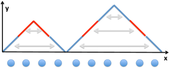
Refer to caption
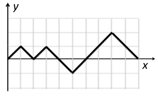
Figure 1: A Dyck walk with s=2𝑠2s=2 colors on a chain of length 2​n=102𝑛102n=10.

Let s𝑠s be a positive integer. An sβˆ’limit-from𝑠s-colored Dyck path from (0,0)00(0,0) to (2n,0(2n,0) is a Dyck path whose steps (1,1)11(1,1) and (1,βˆ’1)11(1,-1) each can have sβ‰₯1𝑠1s\geq 1 different colors. In addition, every step of a given color is uniquely matched with a step down of the same color. Note that s=1𝑠1s=1 corresponds to the standard Dyck paths (see Fig. (1) for an example).

Below, at times, we denote a step up by u≑(1,1)𝑒11u\equiv(1,1) and a step down by d≑(1,βˆ’1)𝑑11d\equiv(1,-1). When there are colorings, we use uksuperscriptπ‘’π‘˜u^{k} and dksuperscriptπ‘‘π‘˜d^{k} to denote a step up and down of color kπ‘˜k, where 1≀k≀s1π‘˜π‘ 1\leq k\leq s.

A peak on the walk is defined to be any coordinate whose height (i.e., yβˆ’limit-from𝑦y-coordinate) is larger than both of its neighbors.

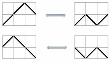
3. Fredkin Markov Chain. The Markov chain in this paper and it predecessors Movassagh2012_brackets ; movassagh2016supercritical have local transition rules. Such Markov chains are said to have Glauber dynamics. Let us describe the uncolored Fredkin Markov chain first as it is more mainstream in the combinatorics community. The state space is the set of Dyck paths, and the Markov chain has the local transition rules shown in Fig. (2). These moves interchange a peak with a step up or down to its left or right. It is important to emphasize that any given Dyck walk can be related to any other by a series of these local moves. Moreover, applying any sequence of these local moves to any given Dyck results in a sequence of Dyck walks only.
Refer to caption
Figure 2: Local transition rules for the Fredkin Markov chain.

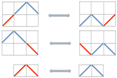
The sβˆ’limit-from𝑠s-colored version is entirely similar except that any peak of a given color can be interchanged with any step up or down step of whatever color. Moreover, there is a transition rule that changes the color of a given peak. Some of these transition rules are shown in Fig. (3).
Refer to caption
Figure 3: Local transition rules for the 2βˆ’limit-from22-colored Fredkin Markov chain. We are only showing exchange of a blue peak with red steps to convey the transition rules with an understanding that there are other moves. Namely, a peak of any given color (here blue or red) can be exchanged with a step down or up of any color (here blue or red).

4. Lower-bound on the gap of Fredkin Markov Chain. We wish to lower bound the spectral gap of the Fredkin Markov chain. Previously we considered another Markov chain on the space of sβˆ’limit-from𝑠s-colored Dyck paths, where the transition rules were as follows:

  1. 1.

    Pick a position between 111 and 2​nβˆ’12𝑛12n-1 on the Dyck path at random.

  2. 2.

    If there is a peak there, remove it to get a path of length 2​nβˆ’22𝑛22n-2.

  3. 3.

    Insert a peak at a random position between 00 and 2​nβˆ’22𝑛22n-2 with a color randomly chosen uniformly out of the s𝑠s possibilities.

The spectral gap of this Markov chain was proved to be 1βˆ’Ξ»1=sπ​n11/21subscriptπœ†1π‘ πœ‹superscript𝑛1121-\lambda_{1}=\frac{s}{\sqrt{\pi}n^{11/2}} movassagh2016supercritical . Let us call this Markov chain peak-displacing.

We use the comparison theorem of Diaconis and Saloff-Coste diaconis1993comparison to lower bound the gap of the sβˆ’limit-from𝑠s-colored Fredkin Markov chain in terms of the known gap of the peak-displacing Markov chain. Let us first describe the comparison theorem. We follow the presentation of diaconis1993comparison .

Suppose P,Ο€π‘ƒπœ‹P,\pi and P~,Ο€~~𝑃~πœ‹\tilde{P},\tilde{\pi} are two reversible Markov chains that are supported on the same state space ΩΩ\Omega. We think of P,Ο€π‘ƒπœ‹P,\pi as the chain whose mixing time or gap is unknown and desired, and think of P~,Ο€~~𝑃~πœ‹\tilde{P},\tilde{\pi} as the chain with known eigenvalues. For each pair of states xβ‰ yπ‘₯𝑦x\neq y with P~​(x,y)>0~𝑃π‘₯𝑦0\tilde{P}(x,y)>0, fix a sequence of steps x=x0,x1,x2,…,xk=yformulae-sequenceπ‘₯subscriptπ‘₯0subscriptπ‘₯1subscriptπ‘₯2…subscriptπ‘₯π‘˜π‘¦x=x_{0},x_{1},x_{2},\dots,x_{k}=y with P​(xi,xi+1)>0𝑃subscriptπ‘₯𝑖subscriptπ‘₯𝑖10P(x_{i},x_{i+1})>0. This sequence of steps defines a path Ξ³x,ysubscript𝛾π‘₯𝑦\gamma_{x,y} on the state space with the length |Ξ³x,y|=ksubscript𝛾π‘₯π‘¦π‘˜|\gamma_{x,y}|=k. Let the set of edges in P𝑃P be E={(x,y); ​P​(x,y)>0}𝐸π‘₯𝑦 𝑃π‘₯𝑦0E=\{(x,y);\text{ }P(x,y)>0\} and the set of edges in P~~𝑃\tilde{P} be E~={(x,y); ​P~​(x,y)>0}~𝐸π‘₯𝑦 ~𝑃π‘₯𝑦0\tilde{E}=\{(x,y);\text{ }\tilde{P}(x,y)>0\}. Moreover, let E~​(e)={(x,y)∈E~; ​e∈γx,y}~𝐸𝑒formulae-sequenceπ‘₯𝑦~𝐸 𝑒subscript𝛾π‘₯𝑦\tilde{E}(e)=\{(x,y)\in\tilde{E};\text{ }e\in\gamma_{x,y}\}, where e∈E𝑒𝐸e\in E. In words, E~​(e)~𝐸𝑒\tilde{E}(e) is the set of paths that contain the edge e𝑒e.

In our case, P~~𝑃\tilde{P} is the peak-displacing Markov chain and P𝑃P is the Fredkin Markov chain.

Theorem.

(Comparison theorem diaconis1993comparison , randall2000analyzing ) Let P~,Ο€~~𝑃~πœ‹\tilde{P},\tilde{\pi} and P,Ο€π‘ƒπœ‹P,\pi be reversible Markov chains on a finite set ΩΩ\Omega. Then

(1βˆ’Ξ»1​(P))β‰₯1A​(1βˆ’Ξ»1​(P~)),1subscriptπœ†1𝑃1𝐴1subscriptπœ†1~𝑃\left(1-\lambda_{1}(P)\right)\geq\frac{1}{A}\left(1-\lambda_{1}(\tilde{P})\right),

where

A=maxzβ‰ w:P​(z,w)β‰ 0⁑{1π​(z)​P​(z,w)β€‹βˆ‘xβ‰ y:(z,w)∈γx,y|Ξ³x,y|​π~​(x)​P~​(x,y)}.𝐴subscript:𝑧𝑀𝑃𝑧𝑀01πœ‹π‘§π‘ƒπ‘§π‘€subscript:π‘₯𝑦𝑧𝑀subscript𝛾π‘₯𝑦subscript𝛾π‘₯𝑦~πœ‹π‘₯~𝑃π‘₯𝑦A=\max_{z\neq w:P(z,w)\neq 0}\left\{\frac{1}{\pi(z)P(z,w)}\sum_{x\neq y:(z,w)\in\gamma_{x,y}}|\gamma_{x,y}|\tilde{\pi}(x)\tilde{P}(x,y)\right\}. (2)
Remark 1.

The quantity A𝐴A depends on the choice of canonical paths {Ξ³x,y}subscript𝛾π‘₯𝑦\{\gamma_{x,y}\} that we are free to choose. They play an important role similar to the canonical path technique that was introduced by Jerrum and Sinclair Sinclair1992 . However, the notion of paths in the comparison theorem is fundamentally different because the paths relate two different Markov chains.

Both the peak-displacing and Fredkin Markov chains have the sβˆ’limit-from𝑠s-colored Dyck paths as their vertex sets. They both have the uniform distribution of all (sβˆ’limit-from𝑠s-colored) Dyck walks as their stationary distribution. However, they have different edge sets E𝐸E and E~~𝐸\tilde{E}.

Lemma 1.

The spectral gap of Fredkin Markov chain is upper bounded by

1βˆ’Ξ»1​(P)β‰₯O​(s​nβˆ’15/2)​ minzβ‰ w​P​(z,w).1subscriptπœ†1𝑃𝑂𝑠superscript𝑛152subscriptΒ min𝑧𝑀𝑃𝑧𝑀1-\lambda_{1}(P)\geq{O(sn^{-15/2})\text{ }\text{min}_{z\neq w}P(z,w)}. (3)
Proof.

Since in our case π​(x)=Ο€~​(x)=sβˆ’n/Cnπœ‹π‘₯~πœ‹π‘₯superscript𝑠𝑛subscript𝐢𝑛\pi(x)=\tilde{\pi}(x)=s^{-n}/C_{n}, where Cnsubscript𝐢𝑛C_{n} is the nthsuperscript𝑛thn^{\text{th}} Catalan number we have

Refer to caption
Refer to caption
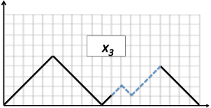
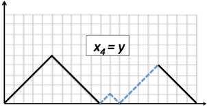
Figure 4: Two adjacent states in peak-displacing Markov chain.
1βˆ’Ξ»1​(P)β‰₯Aβˆ’1​{sπ​n11/2}.1subscriptπœ†1𝑃superscript𝐴1π‘ πœ‹superscript𝑛1121-\lambda_{1}(P)\geq A^{-1}\left\{\frac{s}{\sqrt{\pi}n^{11/2}}\right\}.

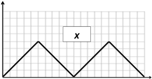
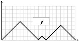
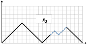
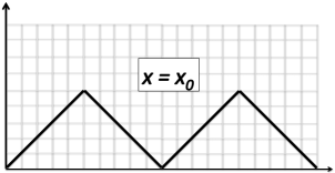
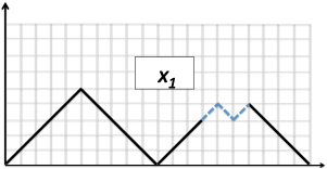
We now define the set of canonical paths. First take the uncolored version s=1𝑠1s=1. Let xπ‘₯x and y𝑦y be two Dyck paths of length 2​n2𝑛2n, where y𝑦y is obtained from xπ‘₯x by randomly cutting a peak and inserting it at a random position. An example of this is shown in Fig. (4), where the right most peak in xπ‘₯x was cut and placed in the valley. Let the initial position of the peak (in xπ‘₯x) be between i𝑖i and i+1𝑖1i+1 and let its final position be between j𝑗j and j+1𝑗1j+1 (in y𝑦y). With no loss of generality take j>i𝑗𝑖j>i and define k=jβˆ’iπ‘˜π‘—π‘–k=j-i. We define the canonical path to be x=x0,x1,…​xk=yformulae-sequenceπ‘₯subscriptπ‘₯0subscriptπ‘₯1…subscriptπ‘₯π‘˜π‘¦x=x_{0},x_{1},\dots x_{k}=y, where each xβ„“subscriptπ‘₯β„“x_{\ell} is a Dyck path that is obtained from xβ„“βˆ’1subscriptπ‘₯β„“1x_{\ell-1} by exchanging the peak with a step to its right. This results in β€œwalking” the peak kπ‘˜k steps to the right until xk=ysubscriptπ‘₯π‘˜π‘¦x_{k}=y. Fig. (5) shows the canonical path that takes xπ‘₯x to y𝑦y, that are adjacent in P𝑃P, shown in Fig. (4).

Turning to the colored case, suppose the peak to be displaced has different colors in xπ‘₯x and y𝑦y. This can easily be implemented in the canonical path by adding a single step at the end of the path which changes the color of the peak at its final position.
Refer to caption
Refer to caption
Refer to caption
Refer to caption
Refer to caption
Figure 5: An example of canonical paths in Fredkin Markov chain with the start state xπ‘₯x and final state y𝑦y.

It remains to upper bound the quantity A𝐴A. It is clear that the length of any canonical path is at most 2​n2𝑛2n. Since Ο€=Ο€~πœ‹~πœ‹\pi=\tilde{\pi}, and choosing a peak at random and inserting at a random position on a chain of length 2​n2𝑛2n with s𝑠s possible choices of random coloring corresponds to P~​(x,y)β‰ˆ1s​(2​n)2~𝑃π‘₯𝑦1𝑠superscript2𝑛2\tilde{P}(x,y)\approx\frac{1}{s\left(2n\right)^{2}}, Eq. (2) is bounded by

A≀maxzβ‰ w:P​(z,w)β‰ 0⁑{2​nP​(z,w)β€‹βˆ‘xβ‰ y:(z,w)∈γx,yP~​(x,y)}≀12​n​s​maxzβ‰ w:P​(z,w)β‰ 0β‘βˆ‘xβ‰ y:(z,w)∈γx,y1P​(z,w)𝐴subscript:𝑧𝑀𝑃𝑧𝑀02𝑛𝑃𝑧𝑀subscript:π‘₯𝑦𝑧𝑀subscript𝛾π‘₯𝑦~𝑃π‘₯𝑦12𝑛𝑠subscript:𝑧𝑀𝑃𝑧𝑀0subscript:π‘₯𝑦𝑧𝑀subscript𝛾π‘₯𝑦1𝑃𝑧𝑀A\leq\max_{z\neq w:P(z,w)\neq 0}\left\{\frac{2n}{P(z,w)}\sum_{x\neq y:(z,w)\in\gamma_{x,y}}\tilde{P}(x,y)\right\}\leq\frac{1}{2ns}\max_{z\neq w:P(z,w)\neq 0}\frac{\sum_{x\neq y:(z,w)\in\gamma_{x,y}}1}{P(z,w)}

The final step is to upper-bound the number of canonical paths going through any edge of Fredkin Markov chain. Suppose (z,w)𝑧𝑀(z,w) is an edge in the a canonical path that maximizes A𝐴A. It is clear that z𝑧z and w𝑀w are equal everywhere except from three consecutive positions corresponding to exchange of a a peak with a single step.

In any canonical path that has (z,w)𝑧𝑀(z,w) as an edge, the peak could have started its motion from, at most, 2​n2𝑛2n places on the path and similarly can terminate its motion in at most 2​n2𝑛2n positions. This gives us O​(n2)𝑂superscript𝑛2O(n^{2}) paths that use the edge with the maximum edge load.

Moreover, there can be at most n𝑛n such peaks whose motion would result in the same edge (z,w)𝑧𝑀(z,w) as we now show. Suppose the edge is the local move that connects π—Œπ–«β€‹Β β€‹u​d​uβ€‹Β β€‹π—Œπ–±subscriptπ—Œπ–«Β π‘’π‘‘π‘’Β subscriptπ—Œπ–±\mathsf{s_{L}}\mbox{ }udu\mbox{ }\mathsf{s_{R}} to π—Œπ–«β€‹Β β€‹u​u​dβ€‹Β β€‹π—Œπ–±subscriptπ—Œπ–«Β π‘’π‘’π‘‘Β subscriptπ—Œπ–±\mathsf{s_{L}}\mbox{ }uud\mbox{ }\mathsf{s_{R}}, where d𝑑d and u𝑒u denote a step down and up, respectively, and π—Œπ–«subscriptπ—Œπ–«\mathsf{s_{L}} and π—Œπ–±subscriptπ—Œπ–±\mathsf{s_{R}} denote a string on the left and a string on the right of the local move, respectively. In this configuration π—Œπ–«subscriptπ—Œπ–«\mathsf{s_{L}} and π—Œπ–±subscriptπ—Œπ–±\mathsf{s_{R}} count once as far as initial and final configurations are concerned; however, they can contribute O​(n)𝑂𝑛O(n) times in the number of paths that use this local move. This can be seen if we take, as an example, π—Œπ–«=u​d​u​d​…​u​dsubscriptπ—Œπ–«π‘’π‘‘π‘’π‘‘β€¦π‘’π‘‘\mathsf{s_{L}}=udud...ud; any of the peaks u​d𝑒𝑑ud could have started walking, leading to the local move. There can be O​(n)𝑂𝑛O(n) choices of such peaks in π—Œπ–«subscriptπ—Œπ–«\mathsf{s_{L}}, all leading to the particular transition described just above.

Therefore, the total number of canonical paths using the maximum edge load is O​(n3)𝑂superscript𝑛3O(n^{3}). In the case that the peak can change color at the last step, this upper bound becomes O​(n3​s)𝑂superscript𝑛3𝑠O(n^{3}s). With this we arrive at the upper-bound on A𝐴A

A≀O​(n2)minzβ‰ w​P​(z,w).𝐴𝑂superscript𝑛2subscriptmin𝑧𝑀𝑃𝑧𝑀A\leq\frac{O(n^{2})}{\text{min}_{z\neq w}P(z,w)}.

Lastly we have the desired bound on the gap

1βˆ’Ξ»1​(P)β‰₯s​ minzβ‰ w​P​(z,w)O​(n15/2).1subscriptπœ†1𝑃𝑠subscriptΒ min𝑧𝑀𝑃𝑧𝑀𝑂superscript𝑛1521-\lambda_{1}(P)\geq\frac{s\text{ }\text{min}_{z\neq w}P(z,w)}{O(n^{15/2})}. (4)

∎

The gap gives us an upper-bound on the mixing time of the Fredkin Markov chain via Eq. (1).

If we take P​(z,w)=1/2𝑃𝑧𝑀12P(z,w)=1/2, then we have a polynomial upper (lower)-bound on the spectral gap (mixing time) of Fredkin Markov chain. In Section III.3 we define a suitable Markov chain in which P​(z,w)∝1/nproportional-to𝑃𝑧𝑀1𝑛P(z,w)\propto 1/n, which also yields a polynomial upper bound.

5. An interesting failed attempt: Wilson’s lattice path Markov chain. In wilson2004mixing , David B. Wilson defines a lattice path from (0,0)00(0,0) to (2n,0(2n,0) to be a connected path with steps (1,1)11(1,1) and (1,βˆ’1)11(1,-1). In other words, a lattice path on 2​n2𝑛2n steps is a walk from left to right between the coordinates (x0,y0)=(0,0)subscriptπ‘₯0subscript𝑦000\left(x_{0},y_{0}\right)=\left(0,0\right) and (x2​n,y2​n)=(2​n,0)subscriptπ‘₯2𝑛subscript𝑦2𝑛2𝑛0\left(x_{2n},y_{2n}\right)=\left(2n,0\right). And at each step the yβˆ’limit-from𝑦y-coordinate changes by one (xi+1,yi+1)=(xi+1,yiΒ±1)subscriptπ‘₯𝑖1subscript𝑦𝑖1subscriptπ‘₯𝑖1plus-or-minussubscript𝑦𝑖1(x_{i+1},y_{i+1})=(x_{i}+1,y_{i}\pm 1). See Fig. (6). In particular, such lattice paths can go below the xβˆ’limit-fromπ‘₯x-axis

Refer to caption
Figure 6: A lattice path through 5Γ—5555\times 5 square.

The lattice path Markov chain is local and has the lattice paths as its state space. The transition rules are as follows: Randomly pick two adjacent steps on the lattice path and if they correspond to a peak then randomly change it to a valley and vice versa. The mixing time of lattice path Markov chain wilson2004mixing , was proven by D.B. Wilson to be Ξ˜β€‹(n3​log⁑n)Θsuperscript𝑛3𝑛\Theta(n^{3}\log n) wilson2004mixing . It is noteworthy that this scaling is exact.

Let positive lattice path Markov chain be a local Markov chain, that has the Dyck paths as its state space. The transition rules are the same as the lattice path Markov chain with the additional condition that if changing a peak to a valley results in the walk crossing the xβˆ’limit-fromπ‘₯x-axis to become negative then the chain will skip that move in that time step (i.e., the chain sits idle). The mixing time that Wilson obtained also upper bounds the mixing time of the positive lattice path Markov chain:

Lemma 2.

The mixing time of positive lattice path Markov chain is upper bounded by O​(n3​log⁑n)𝑂superscript𝑛3𝑛O(n^{3}\log n).

Proof.

The positive lattice path Markov chain has the space of Dyck walks as its possible states, which is a subset of all possible lattice paths. D. J. Aldous’ Theorem says that if Xtsubscript𝑋𝑑X_{t} is a reversible Markov chain on the state space ΩΩ\Omega with the stationary measure Ο€πœ‹\pi and spectral gap ΔΔ\Delta and BβŠ‚Ξ©π΅Ξ©B\subset\Omega is a non-empty subset, then the gap of the chain induced on B𝐡B is Ξ”Bβ‰₯Ξ”subscriptΔ𝐡Δ\Delta_{B}\geq\Delta (see also (levin2009markov, , Theorem 13.20)). Therefore, the spectral gap of lattice path Markov chain lower-bounds the gap of positive lattice path chains. ∎

So it seems quite natural that one would apply the comparison technique to positive lattice path Markov chain and leverage Wilson’s tight bound to ultimately lower bound the spectral gap of the Fredkin Markov chain.
Refer to caption
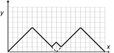
Figure 7: The local move between two adjacent states in the lattice path Markov chain with no corresponding adjacent moves in the Fredkin chain.

Although the Fredkin Markov chain is similar to the positive lattice path Markov chain, it has a crucial difference.

For every Fredkin adjacent move there is a corresponding adjacent move in positive lattice paths. That is, there is a flipping of a peak or valley that relates any two adjacent states under Fredkin Markov chain. In Fig. (2) imagine flipping peaks to valleys and vice versa, then the resulting local moves coincide with Fredkin moves.

However, the converse is not true; there are adjacent states in the positive Markov chain that do not have equivalent adjacent states under the Fredkin Markov chain. In particular, any valley with side lengths of at least 222 has an adjacent state with a single peak at the bottom of the dale under positive Markov chain moves. But the Fredkin Markov chain cannot relate them with a single move. See Fig. (7) for an example of two adjacent states under a positive lattice path Markov chain with no single Fredkin local move that would relate them.

Although we could find paths of length O​(n)𝑂𝑛O(n) to relate the worst case scenario shown in Fig. (7), the bounds on A𝐴A ended up being exponentially large in n𝑛n. This was because exponentially many canonical paths would end up needing to use a single edge. Therefore, in Section III.3 we apply the comparison technique using a different Markov chain that gives us the desired result.

It will be very exciting if, like the lattice path Markov chain, an exact bound is obtained for the Fredkin Markov chain. We leave this problem for future work.

III Hamiltonian Gap of Recent Exactly Solvable Models

III.1 Mapping quantum spin Hamiltonians to classical Markov chains

There is a fascinating bridge between certain classical and quantum statistical mechanical systems. This connection goes beyond the well-known equivalence of certain D𝐷D dimensional quantum systems and (D+1)𝐷1(D+1) dimensional classical systems polyakov1987gauge . Suppose we have a quantum Hamiltonian

H=βˆ‘jHj.𝐻subscript𝑗subscript𝐻𝑗H=\sum_{j}H_{j}. (5)
Definition 1.

H𝐻H is called kβˆ’limit-fromπ‘˜k-local if each Hjsubscript𝐻𝑗H_{j} acts non-trivially only on a constant number (k)k) of particles (e.g, spins). For example a spin chain with nearest neighbors interaction is a 2βˆ’limit-from22-local Hamiltonian.

Definition 2.

H𝐻H is Frustration Free (FF) if the ground state of H𝐻H, which is the eigenvector corresponding to the lowest eigenvalue (ground state energy) of H𝐻H, is also the ground state of every Hjsubscript𝐻𝑗H_{j}.

Definition 3.

H𝐻H is called Stoquastic with respect to a basis ℬℬ{\cal B} if each Hjsubscript𝐻𝑗H_{j} has non-positive off-diagonal entries with respect to ℬℬ{\cal B} bravyi2006complexity .

Definition 4.

The gap of a quantum Hamiltonian H𝐻H is the positive difference of its two smallest eigenvalues and is denoted by Δ​(H)Δ𝐻\Delta(H).

Comment: The definition of the gap is different from the definition in the Markov chain literature, where the gap is the difference of the two largest eigenvalues.

Comment: The usage of Perron-Frobenius theorem in the context of quantum spin systems has a long history. In particular the non-positivity was utilized in Marshall’s paper marshall1955antiferromagnetism and Mattis-Lieb theory lieb1962ordering as well as more recent works aizenman1994geometric . In particular, the stability of the gap along a path that connects the Hamiltonian to an exactly solvable Hamiltonian is a result of positivity.

The term stoquastic is meant to emphasize the connection between classical stochastic matrices and quantum Hamiltonians. Stoquastic Hamiltonians avoid the so called sign problem and their ground state properties can be simulated using classical Monte Carlo algorithms (bravyi2009complexity, , and references therein.). With no loss of generality the smallest eigenvalue of any FF Hamiltonian is taken to be zero and we have H​|ψ⟩=0𝐻ketπœ“0H|\psi\rangle=0, where |ψ⟩ketπœ“|\psi\rangle is the ground state of H𝐻H and FF condition implies that Hj​|ψ⟩=0subscript𝐻𝑗ketπœ“0H_{j}|\psi\rangle=0 for all j𝑗j.

Remark 2.

If we multiply the generator or generating matrix of continuous time Markov chains by minus one, the resulting matrix would be a stoquastic matrix. However, stoquastic matrices may have diagonal entries of any sign.

Using the Perron-Frobenius theorem, Bravyi and Terhal showed that the ground state |ψ⟩ketπœ“|\psi\rangle of any stoquastic FF Hamiltonian can be chosen to be a vector with non-negative amplitudes on a standard basis bravyi2009complexity . Suppose H𝐻H is restricted to the ground subspace. Following bravyi2009complexity let us define the transition matrix

P​(x,y)=Ξ΄x,yβˆ’Ξ²β€‹Ο€β€‹(y)π​(x)β€‹βŸ¨x|H|yβŸ©π‘ƒπ‘₯𝑦subscript𝛿π‘₯π‘¦π›½πœ‹π‘¦πœ‹π‘₯quantum-operator-productπ‘₯𝐻𝑦P(x,y)=\delta_{x,y}-\beta\sqrt{\frac{\pi(y)}{\pi(x)}}\langle x|H|y\rangle (6)

where Ξ²>0𝛽0\beta>0 is real and chosen such that P​(x,y)β‰₯0𝑃π‘₯𝑦0P(x,y)\geq 0 and π​(x)=⟨x|ψ⟩2πœ‹π‘₯superscriptinner-productπ‘₯πœ“2\pi(x)=\langle x|\psi\rangle^{2} is the stationary distribution. The eigenvalue equation (π•€βˆ’Ξ²β€‹H)​|ψ⟩=|ΟˆβŸ©π•€π›½π»ketπœ“ketπœ“(\mathbb{I}-\beta H)|\psi\rangle=|\psi\rangle implies that βˆ‘yP​(x,y)=1subscript𝑦𝑃π‘₯𝑦1\sum_{y}P(x,y)=1. Therefore the matrix P𝑃P really defines a random walk.

Recall that the spectral gap of a Markov chain is the difference of its two largest eigenvalues, i.e. 1βˆ’Ξ»1​(P)1subscriptπœ†1𝑃1-\lambda_{1}(P). Because of the minus sign in Eq. (6) the energy gap of the FF Hamiltonian is related to the gap of the Markov chain by

Δ​(H)=Ξ»1​(P)Ξ².Δ𝐻subscriptπœ†1𝑃𝛽\Delta(H)=\frac{\lambda_{1}(P)}{\beta}.

This provides a powerful tool for quantifying the gap of a class of quantum local Hamiltonians using the arsenal of existing techniques for proving the gap of classical Markov chains.

We will use this connection along with the scaling of the gap proved for the Fredkin Markov chain in the previous section to prove the gap of the Fredkin quantum spin chain model salberger2016fredkin ; dell2016violation .

III.2 The Motzkin spin chain and its ground state
Refer to caption
Figure 8: Labels for the 2​s+12𝑠12s+1 states for s=1𝑠1s=1 and s=2𝑠2s=2. Note that the flat steps are always black for all s𝑠s.

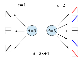
The predecessor of the Fredkin spin chain is the colored Motzkin spin chain movassagh2016supercritical , which we now describe. Throughout we take the length of the chain to be 2​n2𝑛2n. Let us consider an integer spinβˆ’s𝑠-s chain of length 2​n2𝑛2n. It is convenient to label the d=2​s+1𝑑2𝑠1d=2s+1 spin states by steps up and down of s𝑠s different colors as shown in Fig. (8). Equivalently, and for better readability, we instead use the labels {u1,u2,β‹―,us,0,d1,d2,β‹―,ds}superscript𝑒1superscript𝑒2β‹―superscript𝑒𝑠0superscript𝑑1superscript𝑑2β‹―superscript𝑑𝑠\left\{u^{1},u^{2},\cdots,u^{s},0,d^{1},d^{2},\cdots,d^{s}\right\} where u𝑒u means a step up and d𝑑d a step down. We distinguish each type of step by associating a color from the s𝑠s colors shown as superscripts on u𝑒u and d𝑑d.

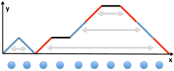
A Motzkin walk on 2​n2𝑛2n steps is any walk from (x,y)=(0,0)π‘₯𝑦00\left(x,y\right)=\left(0,0\right) to (x,y)=(2​n,0)π‘₯𝑦2𝑛0\left(x,y\right)=\left(2n,0\right) with steps (1,0)10\left(1,0\right), (1,1)11\left(1,1\right) and (1,βˆ’1)11\left(1,-1\right) that never passes below the xβˆ’limit-fromπ‘₯x-axis, i.e., yβ‰₯0𝑦0y\geq 0. An example of such a walk is shown in Fig. (9). In our model the unique ground state is the sβˆ’limit-from𝑠s-colored Motzkin state which is defined to be the uniform superposition of all s𝑠s colorings of Motzkin walks on 2​n2𝑛2n steps.

The Schmidt rank is sn+1βˆ’1sβˆ’1β‰ˆsn+1sβˆ’1superscript𝑠𝑛11𝑠1superscript𝑠𝑛1𝑠1\frac{s^{n+1}-1}{s-1}\approx\frac{s^{n+1}}{s-1}, and the half-chain entanglement entropy asymptotically is movassagh2016supercritical

S𝑆\displaystyle S =\displaystyle= 2​log2⁑(s)​ ​2​σπ​ ​n+12​log2⁑(2​π​σ​n)+(Ξ³βˆ’12)​log2⁑ebits2subscript2𝑠 2πœŽπœ‹Β π‘›12subscript22πœ‹πœŽπ‘›π›Ύ12subscript2𝑒bits\displaystyle 2\log_{2}\left(s\right)\mbox{ }\sqrt{\frac{2\sigma}{\pi}}\mbox{ }\sqrt{n}+\frac{1}{2}\log_{2}\left(2\pi\sigma n\right)+\left(\gamma-\frac{1}{2}\right)\log_{2}e\quad\mbox{bits}

where Οƒ=s2​s+1πœŽπ‘ 2𝑠1\sigma=\frac{\sqrt{s}}{2\sqrt{s}+1} and γ𝛾\gamma is Euler’s constant. The ground state is a pure state (the Motzkin state), whose entanglement entropy is zero. However, the entanglement entropy quantifies the amount of disorder produced (i.e., information lost) by ignoring a subset of the chain. The leading order n𝑛\sqrt{n} scaling of the half-chain entropy establishes that there is a large amount of quantum correlations between the two halves.
Refer to caption
Figure 9: A Motzkin walk with s=2𝑠2s=2 colors on a chain of length 2​n=102𝑛102n=10.

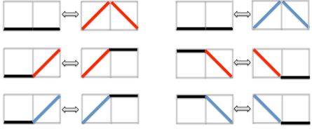
Consider the following local operations to any Motzkin walk: interchanging zero with a non-flat step (i.e., 0​uk↔uk​0↔0superscriptπ‘’π‘˜superscriptπ‘’π‘˜00u^{k}\leftrightarrow u^{k}0 or 0​dk↔dk​0↔0superscriptπ‘‘π‘˜superscriptπ‘‘π‘˜00d^{k}\leftrightarrow d^{k}0) or interchanging a consecutive pair of zeros with a peak of a given color (i.e., 00↔uk​dk↔00superscriptπ‘’π‘˜superscriptπ‘‘π‘˜00\leftrightarrow u^{k}d^{k}). These are shown in Fig. (10). Any sβˆ’limit-from𝑠s-colored Motzkin walk can be obtained from another one by a sequence of these local changes.

To construct a local Hamiltonian with projectors as interactions that has the uniform superposition of the Motzkin walks as its zero energy ground state, each of the local terms of the Hamiltonian has to annihilate states that are symmetric under these interchanges. Physically, local projectors as interactions have the advantage of being robust against certain perturbations Kraus2008 . This is important from a practical point of view and experimental realizations.
Refer to caption
Figure 10: Local moves for s=2𝑠2s=2.

The local Hamiltonian that has the Motzkin state as its unique zero energy ground state is movassagh2016supercritical

H=Ξ b​o​u​n​d​a​r​y+βˆ‘j=12​nβˆ’1Ξ j,j+1+βˆ‘j=12​nβˆ’1Ξ j,j+1c​r​o​s​s,𝐻subscriptΞ π‘π‘œπ‘’π‘›π‘‘π‘Žπ‘Ÿπ‘¦superscriptsubscript𝑗12𝑛1subscriptΠ𝑗𝑗1superscriptsubscript𝑗12𝑛1superscriptsubscriptΠ𝑗𝑗1π‘π‘Ÿπ‘œπ‘ π‘ H=\Pi_{boundary}+\sum_{j=1}^{2n-1}\Pi_{j,j+1}+\sum_{j=1}^{2n-1}\Pi_{j,j+1}^{cross}, (7)

where Ξ j,j+1subscriptΠ𝑗𝑗1\Pi_{j,j+1} implements the local operations discussed above and is defined by

Ξ j,j+1β‰‘βˆ‘k=1s[|Uk⟩j,j+1⟨U|k+|Dk⟩j,j+1⟨Dk|+|Ο†k⟩j,j+1βŸ¨Ο†k|]\Pi_{j,j+1}\equiv\sum_{k=1}^{s}\left[|U^{k}\rangle_{j,j+1}\langle U{}^{k}|+|D^{k}\rangle_{j,j+1}\langle D^{k}|+|\varphi^{k}\rangle_{j,j+1}\langle\varphi^{k}|\right]

with |Uk⟩=12​[|0​ukβŸ©βˆ’|uk​0⟩]ketsuperscriptπ‘ˆπ‘˜12delimited-[]ket0superscriptπ‘’π‘˜ketsuperscriptπ‘’π‘˜0|U^{k}\rangle=\frac{1}{\sqrt{2}}\left[|0u^{k}\rangle-|u^{k}0\rangle\right], |Dk⟩=12​[|0​dkβŸ©βˆ’|dk​0⟩]ketsuperscriptπ·π‘˜12delimited-[]ket0superscriptπ‘‘π‘˜ketsuperscriptπ‘‘π‘˜0|D^{k}\rangle=\frac{1}{\sqrt{2}}\left[|0d^{k}\rangle-|d^{k}0\rangle\right] and |Ο†k⟩=12​[|00βŸ©βˆ’|uk​dk⟩]ketsuperscriptπœ‘π‘˜12delimited-[]ket00ketsuperscriptπ‘’π‘˜superscriptπ‘‘π‘˜|\varphi^{k}\rangle=\frac{1}{\sqrt{2}}\left[|00\rangle-|u^{k}d^{k}\rangle\right]. The term Ξ b​o​u​n​d​a​r​yβ‰‘βˆ‘k=1s[|dk⟩1β€‹βŸ¨dk|+|uk⟩2​nβ€‹βŸ¨uk|]subscriptΞ π‘π‘œπ‘’π‘›π‘‘π‘Žπ‘Ÿπ‘¦superscriptsubscriptπ‘˜1𝑠delimited-[]subscriptketsuperscriptπ‘‘π‘˜1brasuperscriptπ‘‘π‘˜subscriptketsuperscriptπ‘’π‘˜2𝑛brasuperscriptπ‘’π‘˜\Pi_{boundary}\equiv\sum_{k=1}^{s}\left[|d^{k}\rangle_{1}\langle d^{k}|+|u^{k}\rangle_{2n}\langle u^{k}|\right] selects out the Motzkin state by excluding all walks that start and end at non-zero heights. Lastly, Ξ j,j+1c​r​o​s​s=βˆ‘kβ‰ i|uk​di⟩j,j+1β€‹βŸ¨uk​di|superscriptsubscriptΠ𝑗𝑗1π‘π‘Ÿπ‘œπ‘ π‘ subscriptπ‘˜π‘–subscriptketsuperscriptπ‘’π‘˜superscript𝑑𝑖𝑗𝑗1brasuperscriptπ‘’π‘˜superscript𝑑𝑖\Pi_{j,j+1}^{cross}=\sum_{k\neq i}|u^{k}d^{i}\rangle_{j,j+1}\langle u^{k}d^{i}| ensures that balancing is well ordered (i.e., prohibits 00↔uk​di↔00superscriptπ‘’π‘˜superscript𝑑𝑖00\leftrightarrow u^{k}d^{i}); these projectors are required only when s>1𝑠1s>1 and do not appear in Movassagh2012_brackets .

In movassagh2016supercritical we proved that the energy gap to the first excited state is Ξ˜β€‹(nβˆ’c)Θsuperscript𝑛𝑐\Theta(n^{-c}).

III.3 The Fredkin spin chain and its energy gap

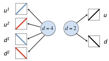
The Fredkin spin chain is a Fermionic extension of movassagh2016supercritical in which d𝑑d is even. The spin states are naturally labeled as shown in See Fig. (11).
Refer to caption
Figure 11: Labeling of the spin states for half-integer spin s𝑠s. Left s=3/2𝑠32s=3/2 and on right s=1/2𝑠12s=1/2.

In salberger2016fredkin , the unique ground state is the sβˆ’limit-from𝑠s-colored Dyck state which is defined to be the uniform superposition of all s𝑠s colored Dyck paths on 2​n2𝑛2n steps. An example of such a path was shown in Fig. (1).

Therefore, the Fredkin spin chain’s unique ground state, denoted by |π’Ÿs⟩ketsuperscriptπ’Ÿπ‘ |{\cal D}^{s}\rangle, is

|π’Ÿs⟩=1Nβ€‹βˆ‘w∈{sβˆ’coloredΒ Dyck walks}|w⟩|{\cal D}^{s}\rangle=\frac{1}{\sqrt{N}}\sum_{\begin{array}[]{c}w\in\{s-\text{colored }\\ \text{Dyck walks}\}\end{array}}|w\rangle

where N=sn​Cn𝑁superscript𝑠𝑛subscript𝐢𝑛N=s^{n}C_{n} is the normalization , with Cnsubscript𝐢𝑛C_{n} denoting the nt​hsuperscriptπ‘›π‘‘β„Žn^{th} Catalan number. The Hamiltonian whose zero energy state is |π’Ÿs⟩ketsuperscriptπ’Ÿπ‘ |{\cal D}^{s}\rangle is 3-local and reads

H=βˆ‘j=12​nβˆ’2Ξ j,j+1,j+2+βˆ‘j=12​nβˆ’1Ξ j,j+1c​r​o​s​s+Ξ b​o​u​n​d​a​r​y𝐻superscriptsubscript𝑗12𝑛2subscriptΠ𝑗𝑗1𝑗2superscriptsubscript𝑗12𝑛1superscriptsubscriptΠ𝑗𝑗1π‘π‘Ÿπ‘œπ‘ π‘ subscriptΞ π‘π‘œπ‘’π‘›π‘‘π‘Žπ‘Ÿπ‘¦H=\sum_{j=1}^{2n-2}\Pi_{j,j+1,j+2}+\sum_{j=1}^{2n-1}\Pi_{j,j+1}^{cross}+\Pi_{boundary} (8)

where

Ξ j,j+1,j+2subscriptΠ𝑗𝑗1𝑗2\displaystyle\Pi_{j,j+1,j+2} =\displaystyle= βˆ‘k1,k2=1s|Uk1,k2⟩j,j+1,j+2β€‹βŸ¨Uk1,k2|+|Dk1,k2⟩j,j+1,j+2β€‹βŸ¨Dk1,k2|+|Ο†k1,k2⟩j,j+1,j+2β€‹βŸ¨Ο†k1,k2|superscriptsubscriptsubscriptπ‘˜1subscriptπ‘˜21𝑠subscriptketsuperscriptπ‘ˆsubscriptπ‘˜1subscriptπ‘˜2𝑗𝑗1𝑗2brasuperscriptπ‘ˆsubscriptπ‘˜1subscriptπ‘˜2subscriptketsuperscript𝐷subscriptπ‘˜1subscriptπ‘˜2𝑗𝑗1𝑗2brasuperscript𝐷subscriptπ‘˜1subscriptπ‘˜2subscriptketsuperscriptπœ‘subscriptπ‘˜1subscriptπ‘˜2𝑗𝑗1𝑗2brasuperscriptπœ‘subscriptπ‘˜1subscriptπ‘˜2\displaystyle\sum_{k_{1},k_{2}=1}^{s}|U^{k_{1},k_{2}}\rangle_{j,j+1,j+2}\langle U^{k_{1},k_{2}}|+|D^{k_{1},k_{2}}\rangle_{j,j+1,j+2}\langle D^{k_{1},k_{2}}|+|\varphi^{k_{1},k_{2}}\rangle_{j,j+1,j+2}\langle\varphi^{k_{1},k_{2}}|
Ξ j,j+1c​r​o​s​ssuperscriptsubscriptΠ𝑗𝑗1π‘π‘Ÿπ‘œπ‘ π‘ \displaystyle\Pi_{j,j+1}^{cross} =\displaystyle= βˆ‘k1β‰ k2=1s|uk1​dk2⟩j,j+1β€‹βŸ¨uk1​dk2|superscriptsubscriptsubscriptπ‘˜1subscriptπ‘˜21𝑠subscriptketsuperscript𝑒subscriptπ‘˜1superscript𝑑subscriptπ‘˜2𝑗𝑗1brasuperscript𝑒subscriptπ‘˜1superscript𝑑subscriptπ‘˜2\displaystyle\sum_{k_{1}\neq k_{2}=1}^{s}|u^{k_{1}}d^{k_{2}}\rangle_{j,j+1}\langle u^{k_{1}}d^{k_{2}}|
Ξ b​o​u​n​d​a​r​ysubscriptΞ π‘π‘œπ‘’π‘›π‘‘π‘Žπ‘Ÿπ‘¦\displaystyle\Pi_{boundary} =\displaystyle= βˆ‘k=1s|dk⟩1β€‹βŸ¨dk|+|uk⟩2​nβ€‹βŸ¨uk|superscriptsubscriptπ‘˜1𝑠subscriptketsuperscriptπ‘‘π‘˜1brasuperscriptπ‘‘π‘˜subscriptketsuperscriptπ‘’π‘˜2𝑛brasuperscriptπ‘’π‘˜\displaystyle\sum_{k=1}^{s}|d^{k}\rangle_{1}\langle d^{k}|+|u^{k}\rangle_{2n}\langle u^{k}|

and |Uk1,k2⟩=12​{|uk1​uk2​dk2βŸ©βˆ’|uk2​dk2​uk1⟩}ketsuperscriptπ‘ˆsubscriptπ‘˜1subscriptπ‘˜212ketsuperscript𝑒subscriptπ‘˜1superscript𝑒subscriptπ‘˜2superscript𝑑subscriptπ‘˜2ketsuperscript𝑒subscriptπ‘˜2superscript𝑑subscriptπ‘˜2superscript𝑒subscriptπ‘˜1|U^{k_{1},k_{2}}\rangle=\frac{1}{\sqrt{2}}\left\{|u^{k_{1}}u^{k_{2}}d^{k_{2}}\rangle-|u^{k_{2}}d^{k_{2}}u^{k_{1}}\rangle\right\} , |Dk1,k2⟩=12​{|dk1​uk2​dk2βŸ©βˆ’|uk2​dk2​dk1⟩}ketsuperscript𝐷subscriptπ‘˜1subscriptπ‘˜212ketsuperscript𝑑subscriptπ‘˜1superscript𝑒subscriptπ‘˜2superscript𝑑subscriptπ‘˜2ketsuperscript𝑒subscriptπ‘˜2superscript𝑑subscriptπ‘˜2superscript𝑑subscriptπ‘˜1|D^{k_{1},k_{2}}\rangle=\frac{1}{\sqrt{2}}\left\{|d^{k_{1}}u^{k_{2}}d^{k_{2}}\rangle-|u^{k_{2}}d^{k_{2}}d^{k_{1}}\rangle\right\} and |Ο†k1,k2⟩=12​{|uk1​dk1βŸ©βˆ’|uk2​dk2⟩}ketsuperscriptπœ‘subscriptπ‘˜1subscriptπ‘˜212ketsuperscript𝑒subscriptπ‘˜1superscript𝑑subscriptπ‘˜1ketsuperscript𝑒subscriptπ‘˜2superscript𝑑subscriptπ‘˜2|\varphi^{k_{1},k_{2}}\rangle=\frac{1}{\sqrt{2}}\left\{|u^{k_{1}}d^{k_{1}}\rangle-|u^{k_{2}}d^{k_{2}}\rangle\right\}, where k1subscriptπ‘˜1k_{1} and k2subscriptπ‘˜2k_{2} denote the colors of each step.

Ξ j,j+1,j+2subscriptΠ𝑗𝑗1𝑗2\Pi_{j,j+1,j+2} in the Hamiltonian implements the Glauber dynamics whose local moves are shown in Fig. (3). The projectors |Uk1,k2βŸ©β€‹βŸ¨Uk1,k2|ketsuperscriptπ‘ˆsubscriptπ‘˜1subscriptπ‘˜2brasuperscriptπ‘ˆsubscriptπ‘˜1subscriptπ‘˜2|U^{k_{1},k_{2}}\rangle\langle U^{k_{1},k_{2}}| and |Dk1,k2βŸ©β€‹βŸ¨Dk1,k2|ketsuperscript𝐷subscriptπ‘˜1subscriptπ‘˜2brasuperscript𝐷subscriptπ‘˜1subscriptπ‘˜2|D^{k_{1},k_{2}}\rangle\langle D^{k_{1},k_{2}}| implement the exchange of a peak with a step up or down and |Ο†k1,k2βŸ©β€‹βŸ¨Ο†k1,k2|ketsuperscriptπœ‘subscriptπ‘˜1subscriptπ‘˜2brasuperscriptπœ‘subscriptπ‘˜1subscriptπ‘˜2|\varphi^{k_{1},k_{2}}\rangle\langle\varphi^{k_{1},k_{2}}| implements the recoloring of a peak (compare with Fig. (3)). βˆ‘jΞ j,j+1c​r​o​s​ssubscript𝑗superscriptsubscriptΠ𝑗𝑗1π‘π‘Ÿπ‘œπ‘ π‘ \sum_{j}\Pi_{j,j+1}^{cross} ensures that the matching steps up and down have the same color. Lastly, Ξ b​o​u​n​d​a​r​ysubscriptΞ π‘π‘œπ‘’π‘›π‘‘π‘Žπ‘Ÿπ‘¦\Pi_{boundary} ensures that the walk always starts and ends at height zero.

Theorem.

The gap of Fredkin spin chain is Δ​(H)=O​(nβˆ’c)Δ𝐻𝑂superscript𝑛𝑐\Delta(H)=O(n^{-c}), with cβ‰₯2𝑐2c\geq 2.

Below we prove this theorem by the following strategy:

1. Upper-bound: Choose a state |Ο•βŸ©ketitalic-Ο•|\phi\rangle which is a uniform superposition of Dyck paths except that each path has a complex phase whose exponent is proportional to the area between the Dyck path and the xβˆ’limit-fromπ‘₯x-axis. We then utilize ideas from universality of Brownian motion and Brownian excursions to prove an O​(nβˆ’2)𝑂superscript𝑛2O(n^{-2}) upper bound on the gap of the Hamiltonian.

2. Lower-bound in the balanced subspace: We restrict the Hamiltonian to the balanced subspace which is the subspace spanned by paths that start at zero height and end at zero height and never become negative. We prove that the gap in this subspace is Δ​(H)β‰₯O​(s​nβˆ’15/2)Δ𝐻𝑂𝑠superscript𝑛152\Delta(H)\geq O(sn^{-15/2}). We obtain this by casting the original Hamiltonian onto a classical Markov chain and then use the results of Section II.

3. Lower-bound in the unbalanced subspace: Prove that the lowest energy in the unbalanced subspace is polynomially small. We achieve this by expressing the Hamiltonian as an effective next-nearest neighbors hopping matrix. We then solve the ground state of the effective Hopping matrix exactly.

III.3.1 The upper-bound on the gap is O​(nβˆ’c)𝑂superscript𝑛𝑐O(n^{-c}), cβ‰₯2𝑐2c\geq 2

Let s=1𝑠1s=1 for now and |Ο•βŸ©ketitalic-Ο•|\phi\rangle be any state with a constant overlap with the zero energy ground state |π’ŸβŸ©ketπ’Ÿ|{\cal D}\rangle. Let |βŸ¨Ο•|D⟩|2≀1/2superscriptinner-productitalic-ϕ𝐷212|\langle\phi|D\rangle|^{2}\leq 1/2; we now show that βŸ¨Ο•|H|Ο•βŸ©β‰₯12​Δ​(H)quantum-operator-productitalic-ϕ𝐻italic-Ο•12Δ𝐻\langle\phi|H|\phi\rangle\geq\frac{1}{2}\Delta(H). First the test state can be written in the orthonormal eigenbasis of the Hamiltonian via

|Ο•βŸ©=Ξ±0​|π’ŸβŸ©+Ξ±1​|e1⟩+β‹―+Ξ±(Cnβˆ’1)​|e(Cnβˆ’1)⟩,ketitalic-Ο•subscript𝛼0ketπ’Ÿsubscript𝛼1ketsubscript𝑒1β‹―subscript𝛼subscript𝐢𝑛1ketsubscript𝑒subscript𝐢𝑛1|\phi\rangle=\alpha_{0}|{\cal D}\rangle+\alpha_{1}|e_{1}\rangle+\dots+\alpha_{(C_{n}-1)}|e_{(C_{n}-1)}\rangle,

where |e1⟩,…,|e(Cnβˆ’1)⟩ketsubscript𝑒1…ketsubscript𝑒subscript𝐢𝑛1|e_{1}\rangle,\dots,|e_{(C_{n}-1)}\rangle are the excited states of H𝐻H. Since |βŸ¨Ο•|D⟩|2≀1/2superscriptinner-productitalic-ϕ𝐷212|\langle\phi|D\rangle|^{2}\leq 1/2 , we have

βŸ¨Ο•|H|Ο•βŸ©=βˆ‘iβ‰₯1|Ξ±i|2β€‹βŸ¨ei|H|ei⟩β‰₯⟨e1|H|e1βŸ©β€‹βˆ‘iβ‰₯1|Ξ±i|2β‰₯12β€‹βŸ¨e1|H|e1⟩,quantum-operator-productitalic-ϕ𝐻italic-Ο•subscript𝑖1superscriptsubscript𝛼𝑖2quantum-operator-productsubscript𝑒𝑖𝐻subscript𝑒𝑖quantum-operator-productsubscript𝑒1𝐻subscript𝑒1subscript𝑖1superscriptsubscript𝛼𝑖212quantum-operator-productsubscript𝑒1𝐻subscript𝑒1\langle\phi|H|\phi\rangle=\sum_{i\geq 1}|\alpha_{i}|^{2}\langle e_{i}|H|e_{i}\rangle\geq\langle e_{1}|H|e_{1}\rangle\sum_{i\geq 1}|\alpha_{i}|^{2}\geq\frac{1}{2}\langle e_{1}|H|e_{1}\rangle,

where Δ​(H)=⟨e1|H|e1βŸ©Ξ”π»quantum-operator-productsubscript𝑒1𝐻subscript𝑒1\Delta(H)=\langle e_{1}|H|e_{1}\rangle is the energy gap. Therefore, all we need is a good test state |Ο•βŸ©ketitalic-Ο•|\phi\rangle with a small overlap with the ground state for which we can prove βŸ¨Ο•|H|Ο•βŸ©β‰₯O​(nβˆ’c)quantum-operator-productitalic-ϕ𝐻italic-ϕ𝑂superscript𝑛𝑐\langle\phi|H|\phi\rangle\geq O(n^{-c}).

Lemma 3.

The gap of Fredkin spin chain, Δ​(H)β‰₯O​(nβˆ’2)Δ𝐻𝑂superscript𝑛2\Delta(H)\geq O(n^{-2}).

Proof.

Let |Ο•βŸ©=1Cnβ€‹βˆ‘π—ŒβˆˆDe2​π​i​A~s​θ~​|π—ŒβŸ©ketitalic-Ο•1subscript𝐢𝑛subscriptπ—Œπ·superscript𝑒2πœ‹π‘–subscript~𝐴𝑠~πœƒketπ—Œ|\phi\rangle=\frac{1}{\sqrt{C_{n}}}\sum_{\mathsf{s}\in D}e^{2\pi i\tilde{A}_{s}\tilde{\theta}}|\mathsf{s}\rangle, and we have

βŸ¨Ο•|D⟩=1Cnβ€‹βˆ‘π—ŒβˆˆDe2​π​i​A~s​θ~inner-productitalic-ϕ𝐷1subscript𝐢𝑛subscriptπ—Œπ·superscript𝑒2πœ‹π‘–subscript~𝐴𝑠~πœƒ\langle\phi|D\rangle=\frac{1}{C_{n}}\sum_{\mathsf{s}\in D}e^{2\pi i\tilde{A}_{s}\tilde{\theta}}

as nβ†’βˆžβ†’π‘›n\rightarrow\infty, the random walk converges to a Wiener process and a random Dyck walk to a Brownian excursion. Currently the length of the walk is over 2​n2𝑛2n steps. We need to map this walk to the interval [0,1]01[0,1] and do so by scaling the walks such that they take the standard form.

Recall that a Brownian excursion, B​(t)𝐡𝑑B(t), is a Brownian motion that takes place on the unit interval, starts and ends at height zero, and never becomes negative. That is, B​(t)𝐡𝑑B(t) is a Brownian motion on the t∈[0,1]𝑑01t\in[0,1], with B​(0)=B​(1)=0𝐡0𝐡10B(0)=B(1)=0 and B​(t)β‰₯0𝐡𝑑0B(t)\geq 0. Let the area below the Brownian excursion be janson2007brownian

Be​x=∫01B​(t)​ ​𝑑t.subscript𝐡𝑒π‘₯superscriptsubscript01𝐡𝑑 differential-d𝑑B_{ex}=\int_{0}^{1}B(t)\mbox{ }dt.

Let fA​(x)subscript𝑓𝐴π‘₯f_{A}(x) be the probability density function of Be​xsubscript𝐡𝑒π‘₯B_{ex}. It is known that (janson2007brownian, , p. 92)

fA​(x)=2​6x2β€‹βˆ‘j=1∞vj2/3​eβˆ’vj​U​(βˆ’54,43;vj)x∈[0,∞)formulae-sequencesubscript𝑓𝐴π‘₯26superscriptπ‘₯2superscriptsubscript𝑗1superscriptsubscript𝑣𝑗23superscript𝑒subscriptπ‘£π‘—π‘ˆ5443subscript𝑣𝑗π‘₯0f_{A}(x)=\frac{2\sqrt{6}}{x^{2}}\sum_{j=1}^{\infty}v_{j}^{2/3}e^{-v_{j}}U(-\frac{5}{4},\frac{4}{3};v_{j})\qquad x\in[0,\infty)

with vj=2​|aj|3/27​x2subscript𝑣𝑗2superscriptsubscriptπ‘Žπ‘—327superscriptπ‘₯2v_{j}=2|a_{j}|^{3}/27x^{2} where ajsubscriptπ‘Žπ‘—a_{j} are the zeros of the Airy function, A​i​(x)𝐴𝑖π‘₯Ai(x), and Uπ‘ˆU is the confluent hypergeometric function. The expected value and standard of deviation of Be​xsubscript𝐡𝑒π‘₯B_{ex}, respectively, are

𝔼​[Be​x]𝔼delimited-[]subscript𝐡𝑒π‘₯\displaystyle\mathbb{E}[B_{ex}] =\displaystyle= 12​π212πœ‹2\displaystyle\frac{1}{2}\sqrt{\frac{\pi}{2}}
ΟƒBe​xsubscript𝜎subscript𝐡𝑒π‘₯\displaystyle\sigma_{B_{ex}} =\displaystyle= 5/12βˆ’Ο€/8.512πœ‹8\displaystyle\sqrt{5/12-\pi/8}.

The sum of the areas of the Dyck paths of length 2​n2𝑛2n is chapman1999moments

A2​n=4nβˆ’12​(2​n+2n+1)∼2​ ​4nπ​(n+1).subscript𝐴2𝑛superscript4𝑛122𝑛2𝑛1similar-to2Β superscript4π‘›πœ‹π‘›1A_{2n}=4^{n}-\frac{1}{2}\left(\begin{array}[]{c}2n+2\\ n+1\end{array}\right)\sim 2\mbox{ }\frac{4^{n}}{\sqrt{\pi(n+1)}}.

Since Cn∼4nn3/2​πsimilar-tosubscript𝐢𝑛superscript4𝑛superscript𝑛32πœ‹C_{n}\sim\frac{4^{n}}{n^{3/2}\sqrt{\pi}}, the expected area is

𝔼​[A~s]=A2​nCnβˆΌΟ€β€‹n3/2.𝔼delimited-[]subscript~𝐴𝑠subscript𝐴2𝑛subscript𝐢𝑛similar-toπœ‹superscript𝑛32\mathbb{E}[\tilde{A}_{s}]=\frac{A_{2n}}{C_{n}}\sim\sqrt{\pi}n^{3/2}.

We now define the scaling constant, c𝑐c, by

𝔼​[A~s]=c​n3/2​𝔼​[Be​x].𝔼delimited-[]subscript~𝐴𝑠𝑐superscript𝑛32𝔼delimited-[]subscript𝐡𝑒π‘₯\mathbb{E}[\tilde{A}_{s}]=cn^{3/2}\mathbb{E}[B_{ex}].

This gives c=2​2𝑐22c=2\sqrt{2}. Make the following change of variables A~p=2​2​n3/2​xsubscript~𝐴𝑝22superscript𝑛32π‘₯\tilde{A}_{p}=2\sqrt{2}n^{3/2}x and ΞΈ~=nβˆ’3/22​2​θ~πœƒsuperscript𝑛3222πœƒ\tilde{\theta}=\frac{n^{-3/2}}{2\sqrt{2}}\theta. With these scalings we have mapped the problem onto a standard Brownian excursion.

The overlap, in the limit, is the characteristic function of the density of the area under the excursion

limnβ†’βˆžβŸ¨π’Ÿ|Ο•βŸ©β‰ˆFA​(ΞΈ)β‰‘βˆ«0∞fA​(x)​e2​π​i​x​θ.subscript→𝑛inner-productπ’Ÿitalic-Ο•subscriptπΉπ΄πœƒsuperscriptsubscript0subscript𝑓𝐴π‘₯superscript𝑒2πœ‹π‘–π‘₯πœƒ\lim_{n\rightarrow\infty}\langle{\cal D}|\phi\rangle\approx F_{A}(\theta)\equiv\int_{0}^{\infty}f_{A}(x)e^{2\pi ix\theta}.

Taking ΞΈ=1/Οƒπœƒ1𝜎\theta=1/\sigma with ΟƒπœŽ\sigma being the standard of deviation, as done in movassagh2016supercritical , we arrive at ΞΈ~=nβˆ’3/22​σ​2=nβˆ’3/210/3βˆ’Ο€~πœƒsuperscript𝑛322𝜎2superscript𝑛32103πœ‹\tilde{\theta}=\frac{n^{-3/2}}{2\sigma\sqrt{2}}=\frac{n^{-3/2}}{\sqrt{10/3-\pi}}.

βˆ‘jβŸ¨Ο•|U⟩j,j+1,j+2β€‹βŸ¨U|Ο•βŸ©subscript𝑗subscriptinner-productitalic-Ο•π‘ˆπ‘—π‘—1𝑗2inner-productπ‘ˆitalic-Ο•\sum_{j}\langle\phi|U\rangle_{j,j+1,j+2}\langle U|\phi\rangle is nonzero only if it relates two walks that differ by a local move at the positions j,j+1,j+2𝑗𝑗1𝑗2j,j+1,j+2. In particular,

βˆ‘jβŸ¨Ο•|U⟩j,j+1,j+2β€‹βŸ¨U|Ο•βŸ©=12​Cnβ€‹βˆ‘j=12​nβˆ’2βˆ‘π—Œ,π—βˆˆDe2​π​i​(A~sβˆ’A~t)​θ~β€‹βŸ¨π—Œ|U⟩j,j+1,j+2β€‹βŸ¨U|π—βŸ©.subscript𝑗subscriptinner-productitalic-Ο•π‘ˆπ‘—π‘—1𝑗2inner-productπ‘ˆitalic-Ο•12subscript𝐢𝑛superscriptsubscript𝑗12𝑛2subscriptπ—Œπ—π·superscript𝑒2πœ‹π‘–subscript~𝐴𝑠subscript~𝐴𝑑~πœƒsubscriptinner-productπ—Œπ‘ˆπ‘—π‘—1𝑗2inner-productπ‘ˆπ—\sum_{j}\langle\phi|U\rangle_{j,j+1,j+2}\langle U|\phi\rangle=\frac{1}{2C_{n}}\sum_{j=1}^{2n-2}\sum_{\mathsf{s,t}\in D}e^{2\pi i\left(\tilde{A}_{s}-\tilde{A}_{t}\right)\tilde{\theta}}\langle\mathsf{s}|U\rangle_{j,j+1,j+2}\langle U|\mathsf{t}\rangle. (9)

The change in the area is either zero or one. There are three types of nonzero contributions per j,j+1,j+2𝑗𝑗1𝑗2j,j+1,j+2 in the foregoing equation

π—Œj,j+1,j+2=𝗍j,j+1,j+2:e2​π​i​(A~sβˆ’A~t)​θ~β€‹βŸ¨π—Œ|U⟩j,j+1,j+2β€‹βŸ¨U|π—βŸ©=1,π—Œj,j+1,j+2=u​d​u𝗍j,j+1,j+2=u​u​d:e2​π​i​(A~sβˆ’A~t)​θ~β€‹βŸ¨π—Œ|U⟩j,j+1,j+2β€‹βŸ¨U|π—βŸ©=βˆ’eβˆ’4​π​i​θ~,π—Œj,j+1,j+2=u​u​d𝗍j,j+1,j+2=u​d​u:e2​π​i​(A~sβˆ’A~t)​θ~β€‹βŸ¨π—Œ|U⟩j,j+1,j+2β€‹βŸ¨U|π—βŸ©=βˆ’e4​π​i​θ~.subscriptπ—Œπ‘—π‘—1𝑗2subscript𝗍𝑗𝑗1𝑗2:superscript𝑒2πœ‹π‘–subscript~𝐴𝑠subscript~𝐴𝑑~πœƒsubscriptinner-productπ—Œπ‘ˆπ‘—π‘—1𝑗2inner-productπ‘ˆπ—1formulae-sequencesubscriptπ—Œπ‘—π‘—1𝑗2𝑒𝑑𝑒subscript𝗍𝑗𝑗1𝑗2𝑒𝑒𝑑:superscript𝑒2πœ‹π‘–subscript~𝐴𝑠subscript~𝐴𝑑~πœƒsubscriptinner-productπ—Œπ‘ˆπ‘—π‘—1𝑗2inner-productπ‘ˆπ—superscript𝑒4πœ‹π‘–~πœƒformulae-sequencesubscriptπ—Œπ‘—π‘—1𝑗2𝑒𝑒𝑑subscript𝗍𝑗𝑗1𝑗2𝑒𝑑𝑒:superscript𝑒2πœ‹π‘–subscript~𝐴𝑠subscript~𝐴𝑑~πœƒsubscriptinner-productπ—Œπ‘ˆπ‘—π‘—1𝑗2inner-productπ‘ˆπ—superscript𝑒4πœ‹π‘–~πœƒ\begin{array}[]{ccc}\mathsf{s}_{j,j+1,j+2}=\mathsf{t}_{j,j+1,j+2}&:&e^{2\pi i\left(\tilde{A}_{s}-\tilde{A}_{t}\right)\tilde{\theta}}\langle\mathsf{s}|U\rangle_{j,j+1,j+2}\langle U|\mathsf{t}\rangle=1,\\ \mathsf{s}_{j,j+1,j+2}=udu\quad\mathsf{t}_{j,j+1,j+2}=uud&:&e^{2\pi i\left(\tilde{A}_{s}-\tilde{A}_{t}\right)\tilde{\theta}}\langle\mathsf{s}|U\rangle_{j,j+1,j+2}\langle U|\mathsf{t}\rangle=-e^{-4\pi i\tilde{\theta}},\\ \mathsf{s}_{j,j+1,j+2}=uud\quad\mathsf{t}_{j,j+1,j+2}=udu&:&e^{2\pi i\left(\tilde{A}_{s}-\tilde{A}_{t}\right)\tilde{\theta}}\langle\mathsf{s}|U\rangle_{j,j+1,j+2}\langle U|\mathsf{t}\rangle=-e^{4\pi i\tilde{\theta}}.\end{array}

The dependence is only on the difference of A~sβˆ’A~tsubscript~𝐴𝑠subscript~𝐴𝑑\tilde{A}_{s}-\tilde{A}_{t} which is zero or two. Using the values of these three cases in Eq. 9, we find

βˆ‘j=12​nβˆ’2βŸ¨Ο•|U⟩j,j+1,j+2β€‹βŸ¨U|Ο•βŸ©=1Cnβ€‹βˆ‘j=12​nβˆ’2aj​[1βˆ’cos⁑(4​π​θ~)]β‰ˆ1Cnβ€‹βˆ‘j=12​nβˆ’28​π2​θ~2​ajsuperscriptsubscript𝑗12𝑛2subscriptinner-productitalic-Ο•π‘ˆπ‘—π‘—1𝑗2inner-productπ‘ˆitalic-Ο•1subscript𝐢𝑛superscriptsubscript𝑗12𝑛2subscriptπ‘Žπ‘—delimited-[]14πœ‹~πœƒ1subscript𝐢𝑛superscriptsubscript𝑗12𝑛28superscriptπœ‹2superscript~πœƒ2subscriptπ‘Žπ‘—\sum_{j=1}^{2n-2}\langle\phi|U\rangle_{j,j+1,j+2}\langle U|\phi\rangle=\frac{1}{C_{n}}\sum_{j=1}^{2n-2}a_{j}\left[1-\cos(4\pi\tilde{\theta})\right]\approx\frac{1}{C_{n}}\sum_{j=1}^{2n-2}8\pi^{2}\tilde{\theta}^{2}a_{j} (10)

where ajsubscriptπ‘Žπ‘—a_{j} is the number of strings that have u​u​d𝑒𝑒𝑑uud or u​d​u𝑒𝑑𝑒udu in their j,j+2,j+2𝑗𝑗2𝑗2j,j+2,j+2 positions. An entirely a similarly calculation gives

βˆ‘jβŸ¨Ο•|D⟩j,j+1,j+2β€‹βŸ¨D|Ο•βŸ©=1Cnβ€‹βˆ‘j=12​nβˆ’2bj​[1βˆ’cos⁑(4​π​θ~)]β‰ˆ1Cnβ€‹βˆ‘j=12​nβˆ’28​π2​θ~2​bjsubscript𝑗subscriptinner-productitalic-ϕ𝐷𝑗𝑗1𝑗2inner-product𝐷italic-Ο•1subscript𝐢𝑛superscriptsubscript𝑗12𝑛2subscript𝑏𝑗delimited-[]14πœ‹~πœƒ1subscript𝐢𝑛superscriptsubscript𝑗12𝑛28superscriptπœ‹2superscript~πœƒ2subscript𝑏𝑗\sum_{j}\langle\phi|D\rangle_{j,j+1,j+2}\langle D|\phi\rangle=\frac{1}{C_{n}}\sum_{j=1}^{2n-2}b_{j}\left[1-\cos(4\pi\tilde{\theta})\right]\approx\frac{1}{C_{n}}\sum_{j=1}^{2n-2}8\pi^{2}\tilde{\theta}^{2}b_{j} (11)

where bjsubscript𝑏𝑗b_{j} is the number of strings that have d​u​d𝑑𝑒𝑑dud or u​d​d𝑒𝑑𝑑udd in their j,j+2,j+2𝑗𝑗2𝑗2j,j+2,j+2 positions. Summing up Eq. (10) and Eq. (11) and recalling that ΞΈ~=nβˆ’3/210/3βˆ’Ο€~πœƒsuperscript𝑛32103πœ‹\tilde{\theta}=\frac{n^{-3/2}}{\sqrt{10/3-\pi}}, we have

βŸ¨Ο•|H|Ο•βŸ©=8​π2Cn​(nβˆ’310/3βˆ’Ο€)β€‹βˆ‘j=12​nβˆ’2aj+bjquantum-operator-productitalic-ϕ𝐻italic-Ο•8superscriptπœ‹2subscript𝐢𝑛superscript𝑛3103πœ‹superscriptsubscript𝑗12𝑛2subscriptπ‘Žπ‘—subscript𝑏𝑗\langle\phi|H|\phi\rangle=\frac{8\pi^{2}}{C_{n}}\left(\frac{n^{-3}}{10/3-\pi}\right)\sum_{j=1}^{2n-2}a_{j}+b_{j}

Since (aj+bj)/Cn=π’ͺ​(1)subscriptπ‘Žπ‘—subscript𝑏𝑗subscript𝐢𝑛π’ͺ1(a_{j}+b_{j})/C_{n}=\mathcal{O}(1) , we have that βŸ¨Ο•|H|Ο•βŸ©=π’ͺ​(nβˆ’2)quantum-operator-productitalic-ϕ𝐻italic-Ο•π’ͺsuperscript𝑛2\langle\phi|H|\phi\rangle=\mathcal{O}(n^{-2}). If we take sβ‰₯1𝑠1s\geq 1, then similar arguments give

βŸ¨Ο•|H|Ο•βŸ©βˆnβˆ’3Cn​snβ€‹βˆ‘j=12​nβˆ’2a~j+b~j∼O​(nβˆ’2).proportional-toquantum-operator-productitalic-ϕ𝐻italic-Ο•superscript𝑛3subscript𝐢𝑛superscript𝑠𝑛superscriptsubscript𝑗12𝑛2subscript~π‘Žπ‘—subscript~𝑏𝑗similar-to𝑂superscript𝑛2\langle\phi|H|\phi\rangle\propto\frac{n^{-3}}{C_{n}s^{n}}\sum_{j=1}^{2n-2}\tilde{a}_{j}+\tilde{b}_{j}\sim O(n^{-2}).

∎

III.3.2 The lower bound on the gap in balanced subspace is O​(nβˆ’15/2)𝑂superscript𝑛152O(n^{-15/2})

For now let us be restricted to the balanced subspace, where all the walks in the superposition start at height zero and end at height zero and never become negative. Moreover all up steps and down steps have correctly ordered matching colors.

In this subspace, |π’Ÿs⟩ketsuperscriptπ’Ÿπ‘ |{\cal D}^{s}\rangle is the unique ground state of the frustration free Hamiltonian

H=βˆ‘j=12​nβˆ’2𝕀djβˆ’1βŠ—{βˆ‘k1,k2=1s|Uk1,k2⟩j,j+1,j+2β€‹βŸ¨Uk1,k2|+|Dk1,k2⟩j,j+1,j+2β€‹βŸ¨Dk1,k2|}βŠ—π•€d2​nβˆ’jβˆ’2,𝐻superscriptsubscript𝑗12𝑛2tensor-productsubscript𝕀superscript𝑑𝑗1superscriptsubscriptsubscriptπ‘˜1subscriptπ‘˜21𝑠subscriptketsuperscriptπ‘ˆsubscriptπ‘˜1subscriptπ‘˜2𝑗𝑗1𝑗2brasuperscriptπ‘ˆsubscriptπ‘˜1subscriptπ‘˜2subscriptketsuperscript𝐷subscriptπ‘˜1subscriptπ‘˜2𝑗𝑗1𝑗2brasuperscript𝐷subscriptπ‘˜1subscriptπ‘˜2subscript𝕀superscript𝑑2𝑛𝑗2H=\sum_{j=1}^{2n-2}\mathbb{I}_{d^{j-1}}\otimes\left\{\sum_{k_{1},k_{2}=1}^{s}|U^{k_{1},k_{2}}\rangle_{j,j+1,j+2}\langle U^{k_{1},k_{2}}|+|D^{k_{1},k_{2}}\rangle_{j,j+1,j+2}\langle D^{k_{1},k_{2}}|\right\}\otimes\mathbb{I}_{d^{2n-j-2}},

where Ξ b​o​u​n​d​a​r​ysubscriptΞ π‘π‘œπ‘’π‘›π‘‘π‘Žπ‘Ÿπ‘¦\Pi_{boundary} and βˆ‘j=12​nβˆ’1Ξ j,j+1c​r​o​s​ssuperscriptsubscript𝑗12𝑛1superscriptsubscriptΠ𝑗𝑗1π‘π‘Ÿπ‘œπ‘ π‘ \sum_{j=1}^{2n-1}\Pi_{j,j+1}^{cross} automatically vanish in the balanced subspace.

The Hamiltonian can be mapped to a classical Markov chain, denoted by the matrix P𝑃P, with the entries

P​(𝗍,π—Œ)=Ξ΄π—Œ,π—βˆ’12​s​(nβˆ’1)​π​(π—Œ)π​(𝗍)β€‹βŸ¨π—|H|π—ŒβŸ©,π‘ƒπ—π—Œsubscriptπ›Ώπ—Œπ—12𝑠𝑛1πœ‹π—Œπœ‹π—quantum-operator-productπ—π»π—ŒP(\mathsf{t,s})=\delta_{\mathsf{s,t}}-\frac{1}{2s(n-1)}\sqrt{\frac{\pi(\mathsf{s})}{\pi(\mathsf{t})}}\langle\mathsf{t}|H|\mathsf{s}\rangle, (12)

where π​(π—Œ)β‰‘βŸ¨π—Œ|π’ŸβŸ©2=sβˆ’n​Cnβˆ’1πœ‹π—Œsuperscriptinner-productπ—Œπ’Ÿ2superscript𝑠𝑛superscriptsubscript𝐢𝑛1\pi(\mathsf{s})\equiv\langle\mathsf{s}|{\cal D}\rangle^{2}=s^{-n}C_{n}^{-1} is the stationary distribution. Note that the gap of the Hamiltonian is now related to the spectral gap of the Markov chain (because of the minus sign). Denote the gap by Δ​(H)Δ𝐻\Delta(H). Since they are related by a similarity transformation, we have that

Δ​(H)=2​s​(nβˆ’1)​(1βˆ’Ξ»2​(P)).Δ𝐻2𝑠𝑛11subscriptπœ†2𝑃\Delta(H)=2s(n-1)(1-\lambda_{2}(P)). (13)

Since π​(π—Œ)=π​(𝗍)πœ‹π—Œπœ‹π—\pi(\mathsf{s})=\pi(\mathsf{t}), the Markov chain takes the simpler form

P​(𝗍,π—Œ)π‘ƒπ—π—Œ\displaystyle P(\mathsf{t,s}) =\displaystyle= Ξ΄π—Œ,π—βˆ’12​s​(nβˆ’1)β€‹βŸ¨π—|H|π—ŒβŸ©,subscriptπ›Ώπ—Œπ—12𝑠𝑛1quantum-operator-productπ—π»π—Œ\displaystyle\delta_{\mathsf{s,t}}-\frac{1}{2s(n-1)}\langle\mathsf{t}|H|\mathsf{s}\rangle, (14)
Lemma 4.

P𝑃P defined by Eq. (14) is a reversible Markov chain

Proof.

1. P𝑃P is stochastic. The row sums are equal to one:

βˆ‘π—ŒP​(𝗍,π—Œ)subscriptπ—Œπ‘ƒπ—π—Œ\displaystyle\sum_{\mathsf{s}}P(\mathsf{t,s}) =\displaystyle= βˆ‘π—Œ{Ξ΄π—Œ,π—βˆ’12​s​(nβˆ’1)β€‹βŸ¨π—|H|π—ŒβŸ©}=1βˆ’βˆ‘π—ŒΟ€β€‹(𝗍)βˆ’1/22​s​(nβˆ’1)β€‹βŸ¨π—|H|π—ŒβŸ©β€‹Ο€β€‹(π—Œ)subscriptπ—Œsubscriptπ›Ώπ—Œπ—12𝑠𝑛1quantum-operator-productπ—π»π—Œ1subscriptπ—Œπœ‹superscript𝗍122𝑠𝑛1quantum-operator-productπ—π»π—Œπœ‹π—Œ\displaystyle\sum_{\mathsf{s}}\{\delta_{\mathsf{s,t}}-\frac{1}{2s(n-1)}\langle\mathsf{t}|H|\mathsf{s}\rangle\}=1-\sum_{\mathsf{s}}\frac{\pi(\mathsf{t})^{-1/2}}{2s(n-1)}\langle\mathsf{t}|H|\mathsf{s}\rangle\sqrt{\pi(\mathsf{s})}
=\displaystyle= 1βˆ’Ο€β€‹(𝗍)βˆ’1/22​s​(nβˆ’1)β€‹βˆ‘π—ŒβŸ¨π—|H|π—ŒβŸ©β€‹βŸ¨π—Œ|π’ŸβŸ©=1βˆ’Ο€β€‹(𝗍)βˆ’1/22​s​(nβˆ’1)β€‹βˆ‘π—ŒβŸ¨π—|H|π’ŸβŸ©=11πœ‹superscript𝗍122𝑠𝑛1subscriptπ—Œquantum-operator-productπ—π»π—Œinner-productπ—Œπ’Ÿ1πœ‹superscript𝗍122𝑠𝑛1subscriptπ—Œquantum-operator-productπ—π»π’Ÿ1\displaystyle 1-\frac{\pi(\mathsf{t})^{-1/2}}{2s(n-1)}\sum_{\mathsf{s}}\langle\mathsf{t}|H|\mathsf{s}\rangle\langle\mathsf{s}|{\cal D}\rangle=1-\frac{\pi(\mathsf{t})^{-1/2}}{2s(n-1)}\sum_{\mathsf{s}}\langle\mathsf{t}|H|{\cal D}\rangle=1

where we used the completeness βˆ‘π—Œ|π—ŒβŸ©β€‹βŸ¨π—Œ|=1subscriptπ—Œketπ—Œbraπ—Œ1\sum_{\mathsf{s}}|\mathsf{s}\rangle\langle\mathsf{s}|=1 and the fact that H​|π’Ÿs⟩=0𝐻ketsuperscriptπ’Ÿπ‘ 0H|{\cal D}^{s}\rangle=0 as |π’Ÿs⟩ketsuperscriptπ’Ÿπ‘ |{\cal D}^{s}\rangle is the zero energy ground state of H𝐻H. Therefore, P𝑃P has row sums equal to one.

2. P𝑃P has a unique stationary state:

βˆ‘π—Ο€β€‹(𝗍)​P​(𝗍,π—Œ)subscriptπ—πœ‹π—π‘ƒπ—π—Œ\displaystyle\sum_{\mathsf{t}}\pi(\mathsf{t})P(\mathsf{t,s}) =\displaystyle= π​(π—Œ)βˆ’βˆ‘π—12​s​(nβˆ’1)​π​(π—Œ)​π​(𝗍)β€‹βŸ¨π—|H|π—ŒβŸ©=π​(π—Œ)βˆ’βˆ‘π—12​s​(nβˆ’1)β€‹βŸ¨π—|π’ŸsβŸ©β€‹βŸ¨π—|H|π—ŒβŸ©β€‹βŸ¨π—Œ|π’ŸsβŸ©πœ‹π—Œsubscript𝗍12𝑠𝑛1πœ‹π—Œπœ‹π—quantum-operator-productπ—π»π—Œπœ‹π—Œsubscript𝗍12𝑠𝑛1inner-product𝗍superscriptπ’Ÿπ‘ quantum-operator-productπ—π»π—Œinner-productπ—Œsuperscriptπ’Ÿπ‘ \displaystyle\pi(\mathsf{s})-\sum_{\mathsf{t}}\frac{1}{2s(n-1)}\sqrt{\pi(\mathsf{s})\pi(\mathsf{t})}\langle\mathsf{t}|H|\mathsf{s}\rangle=\pi(\mathsf{s})-\sum_{\mathsf{t}}\frac{1}{2s(n-1)}\langle\mathsf{t}|{\cal D}^{s}\rangle\langle\mathsf{t}|H|\mathsf{s}\rangle\langle\mathsf{s}|{\cal D}^{s}\rangle
=\displaystyle= π​(π—Œ)βˆ’βˆ‘π—12​s​(nβˆ’1)​1Cn​sn/2β€‹βŸ¨π—|H|π—ŒβŸ©β€‹βŸ¨π—Œ|π’Ÿs⟩=π​(π—Œ)βˆ’12​s​(nβˆ’1)β€‹βŸ¨π’Ÿs|H|π—ŒβŸ©β€‹βŸ¨π—Œ|π’Ÿs⟩=π​(π—Œ)πœ‹π—Œsubscript𝗍12𝑠𝑛11subscript𝐢𝑛superscript𝑠𝑛2quantum-operator-productπ—π»π—Œinner-productπ—Œsuperscriptπ’Ÿπ‘ πœ‹π—Œ12𝑠𝑛1quantum-operator-productsuperscriptπ’Ÿπ‘ π»π—Œinner-productπ—Œsuperscriptπ’Ÿπ‘ πœ‹π—Œ\displaystyle\pi(\mathsf{s})-\sum_{\mathsf{t}}\frac{1}{2s(n-1)}\frac{1}{\sqrt{C_{n}}s^{n/2}}\langle\mathsf{t}|H|\mathsf{s}\rangle\langle\mathsf{s}|{\cal D}^{s}\rangle=\pi(\mathsf{s})-\frac{1}{2s(n-1)}\langle\mathsf{{\cal D}}^{s}|H|\mathsf{s}\rangle\langle\mathsf{s}|{\cal D}^{s}\rangle=\pi(\mathsf{s})

3. P𝑃P is reversible. Noting that π​(𝗍)=π​(π—Œ)πœ‹π—πœ‹π—Œ\pi(\mathsf{t})=\pi(\mathsf{s}) and , βŸ¨π—|H|π—ŒβŸ©=βŸ¨π—Œ|H|π—βŸ©,quantum-operator-productπ—π»π—Œquantum-operator-productπ—Œπ»π—\langle\mathsf{t}|H|\mathsf{s}\rangle=\langle\mathsf{s}|H|\mathsf{t}\rangle, it is easy to check that π​(𝗍)​P​(𝗍,π—Œ)=π​(π—Œ)​P​(π—Œ,𝗍)πœ‹π—π‘ƒπ—π—Œπœ‹π—Œπ‘ƒπ—Œπ—\pi(\mathsf{t})P(\mathsf{t,s})=\pi(\mathsf{s})P(\mathsf{s,t}). ∎

Lemma 5.

P​(π—Œ,π—Œ)β‰₯1/2π‘ƒπ—Œπ—Œ12P(\mathsf{s},\mathsf{s})\geq 1/2 and for π—Œβ‰ π—π—Œπ—\mathsf{s}\neq\mathsf{t}, P​(𝗍,π—Œ)π‘ƒπ—π—ŒP(\mathsf{t},\mathsf{s}) is nonzero if only if 𝗍𝗍\mathsf{t} and π—Œπ—Œ\mathsf{s} differ by moving a peak by one position, in which case its value is

P​(𝗍,π—Œ)=14​s​(nβˆ’1).π‘ƒπ—π—Œ14𝑠𝑛1P(\mathsf{t},\mathsf{s})=\frac{1}{4s(n-1)}.
Proof.

From Eq. (14) we have P​(π—Œ,π—Œ)=1βˆ’12​s​(nβˆ’1)β€‹βŸ¨π—Œ|H|π—ŒβŸ©β‰₯1/2π‘ƒπ—Œπ—Œ112𝑠𝑛1quantum-operator-productπ—Œπ»π—Œ12P(\mathsf{s},\mathsf{s})=1-\frac{1}{2s(n-1)}\langle\mathsf{s}|H|\mathsf{s}\rangle\geq 1/2 since βŸ¨π—Œ|H|π—ŒβŸ©β‰€(nβˆ’1)quantum-operator-productπ—Œπ»π—Œπ‘›1\langle\mathsf{s}|H|\mathsf{s}\rangle\leq(n-1). Now take π—β‰ π—Œπ—π—Œ\mathsf{t}\neq\mathsf{s}: it is clear that if π—Œπ—Œ\mathsf{s} differs from 𝗍𝗍\mathsf{t} in more than three consecutive positions then P​(π—Œ,𝗍)=0π‘ƒπ—Œπ—0P(\mathsf{s},\mathsf{t})=0. Therefore P​(π—Œ,𝗍)π‘ƒπ—Œπ—P(\mathsf{s},\mathsf{t}) is nonzero if and only if 𝗍𝗍\mathsf{t} is obtained from π—Œπ—Œ\mathsf{s} by moving a single peak by one position. Now suppose π—Œπ—Œ\mathsf{s} is obtained from 𝗍𝗍\mathsf{t} by moving a single peak. Then for any local move that moves only a single peak and leaves the rest of the positions equal we have βŸ¨π—Œ|H|π—βŸ©=βˆ’1/2quantum-operator-productπ—Œπ»π—12\langle\mathsf{s}|H|\mathsf{t}\rangle=-1/2. Suppose π—Œπ—Œ\mathsf{s} and 𝗍𝗍\mathsf{t} differ at positions j,j+1,j+2𝑗𝑗1𝑗2j,j+1,j+2, then

P​(π—Œ,𝗍)π‘ƒπ—Œπ—\displaystyle P(\mathsf{s},\mathsf{t}) =\displaystyle= βˆ’12​s​(nβˆ’1)β€‹βˆ‘j=12​nβˆ’2βŸ¨π—Œ|​𝕀djβˆ’1βŠ—{|U⟩j,j+1,j+2β€‹βŸ¨U|+|D⟩j,j+1,j+2β€‹βŸ¨D|}βŠ—π•€d2​nβˆ’jβˆ’2​|π—βŸ©12𝑠𝑛1superscriptsubscript𝑗12𝑛2tensor-productbraπ—Œsubscript𝕀superscript𝑑𝑗1subscriptketπ‘ˆπ‘—π‘—1𝑗2braπ‘ˆsubscriptket𝐷𝑗𝑗1𝑗2bra𝐷subscript𝕀superscript𝑑2𝑛𝑗2ket𝗍\displaystyle-\frac{1}{2s(n-1)}\sum_{j=1}^{2n-2}\langle\mathsf{s}|\mathbb{I}_{d^{j-1}}\otimes\left\{|U\rangle_{j,j+1,j+2}\langle U|+|D\rangle_{j,j+1,j+2}\langle D|\right\}\otimes\mathbb{I}_{d^{2n-j-2}}|\mathsf{t}\rangle
=\displaystyle= βˆ’12​s​(nβˆ’1)β€‹βŸ¨π—Œ|​𝕀djβˆ’1βŠ—{|U⟩j,j+1,j+2β€‹βŸ¨U|+|D⟩j,j+1,j+2β€‹βŸ¨D|}βŠ—π•€d2​nβˆ’jβˆ’2​|π—βŸ©=14​s​(nβˆ’1).tensor-product12𝑠𝑛1braπ—Œsubscript𝕀superscript𝑑𝑗1subscriptketπ‘ˆπ‘—π‘—1𝑗2braπ‘ˆsubscriptket𝐷𝑗𝑗1𝑗2bra𝐷subscript𝕀superscript𝑑2𝑛𝑗2ket𝗍14𝑠𝑛1\displaystyle-\frac{1}{2s(n-1)}\langle\mathsf{s}|\mathbb{I}_{d^{j-1}}\otimes\left\{|U\rangle_{j,j+1,j+2}\langle U|+|D\rangle_{j,j+1,j+2}\langle D|\right\}\otimes\mathbb{I}_{d^{2n-j-2}}|\mathsf{t}\rangle=\frac{1}{4s(n-1)}.

∎

Using Eqs. (4) and (13) the lower bound on the gap in the balanced subspace is

Δ​(H)β‰₯O​(s​nβˆ’15/2).Δ𝐻𝑂𝑠superscript𝑛152\Delta(H)\geq O(sn^{-15/2}). (16)

It remains to lower bound the smallest eigenvalues restricted to the unbalanced subspace.

III.3.3 The smallest energy in the unbalanced subspace is O​(nβˆ’c)𝑂superscript𝑛𝑐O(n^{-c}), c≫1much-greater-than𝑐1c\gg 1

Above we proved a polynomial gap to the first excited state by restricting the Hamiltonian to a balanced subspace where no penalties result from boundary terms (i.e., height imbalance) or any of the Ξ j,j+1c​r​o​s​ssuperscriptsubscriptΠ𝑗𝑗1π‘π‘Ÿπ‘œπ‘ π‘ \Pi_{j,j+1}^{cross}’s (i.e., mismatching of colors). We now prove a polynomially small lower bound on the energies of the states in the unbalanced subspace.

Lemma 6.

The ground state energies (smallest eigenvalues) of the Hamiltonian restricted to the unbalanced subspace are at least O​(nβˆ’c)𝑂superscript𝑛𝑐O(n^{-c}) with c≫1much-greater-than𝑐1c\gg 1.

Proof.

We separate the proof into two parts: 1. height-balanced subspace with only mismatched colors and 2. height-imbalance subspace without any mismatches. Simultaneous occurrence of these penalties only increases the energy.

Color mismatching only: In this case the penalty is only due to βˆ‘jΞ j,j+1c​r​o​s​ssubscript𝑗superscriptsubscriptΠ𝑗𝑗1π‘π‘Ÿπ‘œπ‘ π‘ \sum_{j}\Pi_{j,j+1}^{cross} as all the states have zero initial and final heights and they automatically vanish at the boundaries. The Hamiltonian restricted to this space is

H=βˆ‘jΞ j,j+1,j+2+βˆ‘jΞ j,j+1c​r​o​s​s.𝐻subscript𝑗subscriptΠ𝑗𝑗1𝑗2subscript𝑗superscriptsubscriptΠ𝑗𝑗1π‘π‘Ÿπ‘œπ‘ π‘ H=\sum_{j}\Pi_{j,j+1,j+2}+\sum_{j}\Pi_{j,j+1}^{cross}.

Assume we have the minimum (a single mismatch) resulting in the smallest energy penalty. For example we can have w0​u1​w1​u2​w3​d1​w4​d2​w5subscript𝑀0superscript𝑒1subscript𝑀1superscript𝑒2subscript𝑀3superscript𝑑1subscript𝑀4superscript𝑑2subscript𝑀5w_{0}u^{1}w_{1}u^{2}w_{3}d^{1}w_{4}d^{2}w_{5}, where w0,…,w5subscript𝑀0…subscript𝑀5w_{0},\dots,w_{5} are balanced sβˆ’limit-from𝑠s-colored Dyck walks and u1superscript𝑒1u^{1} and u2superscript𝑒2u^{2} are step ups of two different colors being balanced by d1superscript𝑑1d^{1} and d2superscript𝑑2d^{2}, respectively (hence a mismatch of colors). Suppose u2superscript𝑒2u^{2} is at the site i𝑖i and d2superscript𝑑2d^{2} is at the site kπ‘˜k. Now take the amplitude of Ξ i,i+1,i+2subscriptΠ𝑖𝑖1𝑖2\Pi_{i,i+1,i+2} and Ξ iβˆ’1,i,i+1subscriptΠ𝑖1𝑖𝑖1\Pi_{i-1,i,i+1} to zero which would pin u2superscript𝑒2u^{2} to remain at site i𝑖i and overall lower the energy. Also let’s take the amplitude of Ξ k,k+1,k+2subscriptΞ π‘˜π‘˜1π‘˜2\Pi_{k,k+1,k+2} and Ξ kβˆ’1,k,k+1subscriptΞ π‘˜1π‘˜π‘˜1\Pi_{k-1,k,k+1} to zero as to pin d2superscript𝑑2d^{2} at site kπ‘˜k. This reduces the problem to a chain of length kβˆ’iπ‘˜π‘–k-i with a single imbalance d1superscript𝑑1d^{1}. Therefore, a polynomial lower bound on the smallest energy of height-imbalance (only) subspaces lower bounds the purely mismatched subspace. So we now turn to lower bounding the smallest energy of the subspace with only a height-imbalanced.

Height imbalance only: In this subspace Ξ j,j+1c​r​o​s​ssuperscriptsubscriptΠ𝑗𝑗1π‘π‘Ÿπ‘œπ‘ π‘ \Pi_{j,j+1}^{cross} automatically vanishes on any state. So the Hamiltonian restricted to this subspace is

H=βˆ‘jΞ j,j+1,j+2+Ξ b​o​u​n​d​a​r​y.𝐻subscript𝑗subscriptΠ𝑗𝑗1𝑗2subscriptΞ π‘π‘œπ‘’π‘›π‘‘π‘Žπ‘Ÿπ‘¦H=\sum_{j}\Pi_{j,j+1,j+2}+\Pi_{boundary}.

Our goal is to give nβˆ’π’ͺ​(1)superscript𝑛π’ͺ1n^{-\mathcal{O}(1)} lower bound to the minimum energy in the subspace where there are p>0𝑝0p>0 extra down and q>0π‘ž0q>0 extra up steps. Any string on the imbalanced subspace is uniquely written as

π—Œ=w0​dβˆ™β€‹w1​dβˆ™β€‹β€¦β€‹dβˆ™β€‹wp​w0​uβˆ™β€‹v1​uβˆ™β€‹v2​…​uβˆ™β€‹vqπ—Œsubscript𝑀0superscriptπ‘‘βˆ™subscript𝑀1superscriptπ‘‘βˆ™β€¦superscriptπ‘‘βˆ™subscript𝑀𝑝subscript𝑀0superscriptπ‘’βˆ™subscript𝑣1superscriptπ‘’βˆ™subscript𝑣2…superscriptπ‘’βˆ™subscriptπ‘£π‘ž\mathsf{s}=w_{0}d^{\centerdot}w_{1}d^{\centerdot}\dots d^{\centerdot}w_{p}w_{0}u^{\centerdot}v_{1}u^{\centerdot}v_{2}\dots u^{\centerdot}v_{q}

where wisubscript𝑀𝑖w_{i} and visubscript𝑣𝑖v_{i} are colored-Dyck walks and dβˆ™superscriptπ‘‘βˆ™d^{\centerdot} and uβˆ™superscriptπ‘’βˆ™u^{\centerdot} denote the unmatched steps down and up of any color, respectively. Since Dyck walks are of even length, it is clear that p+qπ‘π‘žp+q must be even.

Because of symmetry it is sufficient to consider p>0𝑝0p>0 only, where there are only imbalance down steps. We can omit the boundary terms |uk⟩2​nβ€‹βŸ¨uk|subscriptketsuperscriptπ‘’π‘˜2𝑛brasuperscriptπ‘’π‘˜|u^{k}\rangle_{2n}\langle u^{k}|, which only decreases the energy. Our Hamiltonian becomes

H=βˆ‘jΞ j,j+1,j+2+βˆ‘k=1s|dk⟩1β€‹βŸ¨dk|,𝐻subscript𝑗subscriptΠ𝑗𝑗1𝑗2superscriptsubscriptπ‘˜1𝑠subscriptketsuperscriptπ‘‘π‘˜1brasuperscriptπ‘‘π‘˜H=\sum_{j}\Pi_{j,j+1,j+2}+\sum_{k=1}^{s}|d^{k}\rangle_{1}\langle d^{k}|,

where Ξ j,j+1,j+2subscriptΠ𝑗𝑗1𝑗2\Pi_{j,j+1,j+2} is as before. Note that for a chain of length 2​n2𝑛2n the number of imbalances needs to be even. Assume we have the minimum violation due to a height imbalance at the boundary and let’s focus on a string with a single step up imbalance denoted by w0​dk​w1​dk​w2subscript𝑀0superscriptπ‘‘π‘˜subscript𝑀1superscriptπ‘‘π‘˜subscript𝑀2w_{0}d^{k}w_{1}d^{k}w_{2}, where as before w0subscript𝑀0w_{0}, w1subscript𝑀1w_{1} and w2subscript𝑀2w_{2} are balanced sβˆ’limit-from𝑠s-colored Dyck walks and dksuperscriptπ‘‘π‘˜d^{k} is a step of color k∈{1,…,s}π‘˜1…𝑠k\in\{1,\dots,s\}. This allows us to drop βˆ‘k=1s|uk⟩2​nβ€‹βŸ¨uk|superscriptsubscriptπ‘˜1𝑠subscriptketsuperscriptπ‘’π‘˜2𝑛brasuperscriptπ‘’π‘˜\sum_{k=1}^{s}|u^{k}\rangle_{2n}\langle u^{k}|, which only decreases the energy. Let us denote the first imbalanced dksuperscriptπ‘‘π‘˜d^{k} by xπ‘₯x and the rest of the imbalanced steps by y𝑦y, then the Hamiltonians is

Hx=|x⟩1β€‹βŸ¨x|+βˆ‘jΞ j,j+1,j+2+Θj,j+1,j+2x+Θj,j+1,j+2y,superscript𝐻π‘₯subscriptketπ‘₯1braπ‘₯subscript𝑗subscriptΠ𝑗𝑗1𝑗2superscriptsubscriptΞ˜π‘—π‘—1𝑗2π‘₯superscriptsubscriptΞ˜π‘—π‘—1𝑗2𝑦H^{x}=|x\rangle_{1}\langle x|+\sum_{j}\Pi_{j,j+1,j+2}+\Theta_{j,j+1,j+2}^{x}+\Theta_{j,j+1,j+2}^{y},

where Θj,j+1,j+2xsuperscriptsubscriptΞ˜π‘—π‘—1𝑗2π‘₯\Theta_{j,j+1,j+2}^{x} is the projector that spans βˆ‘k=1s12​(|uk​dk​xβŸ©βˆ’|x​uk​dk⟩)superscriptsubscriptπ‘˜1𝑠12ketsuperscriptπ‘’π‘˜superscriptπ‘‘π‘˜π‘₯ketπ‘₯superscriptπ‘’π‘˜superscriptπ‘‘π‘˜\sum_{k=1}^{s}\frac{1}{\sqrt{2}}\left(|u^{k}d^{k}x\rangle-|xu^{k}d^{k}\rangle\right) and Θj,j+1,j+2ysuperscriptsubscriptΞ˜π‘—π‘—1𝑗2𝑦\Theta_{j,j+1,j+2}^{y} projects onto βˆ‘k=1s12​(|uk​dk​yβŸ©βˆ’|y​uk​dk⟩)superscriptsubscriptπ‘˜1𝑠12ketsuperscriptπ‘’π‘˜superscriptπ‘‘π‘˜π‘¦ket𝑦superscriptπ‘’π‘˜superscriptπ‘‘π‘˜\sum_{k=1}^{s}\frac{1}{\sqrt{2}}\left(|u^{k}d^{k}y\rangle-|yu^{k}d^{k}\rangle\right). We only have |xβŸ©β€‹βŸ¨x|ketπ‘₯braπ‘₯|x\rangle\langle x| as a y𝑦y step can never pass to the left of the xπ‘₯x down step. We think of xπ‘₯x and y𝑦y steps as ’particles’ that can move on the chain. In any configuration of y𝑦y particles, the xπ‘₯x particle vanishes upon touching any y𝑦y; therefore y𝑦y particles serve as kind of domain walls for xπ‘₯x. Since our goal is to get a lower bound on the energy, we can only analyze the interval between 111 and the first y𝑦y particle which is located in the position mπ‘šm which is between the position of xπ‘₯x and 2​n2𝑛2n. So we can equivalently define the length of the chain to be mπ‘šm and analyze a single imbalance (i.e., xπ‘₯x) on this chain. Since, we have a single imbalance, mπ‘šm necessarily is odd.

The Hilbert space now is the span of

|π—ŒβŸ©βŠ—|x⟩jβŠ—|π—βŸ©,whereΒ π—Œβˆˆπ’Ÿjβˆ’1s​ andΒ β€‹π—βˆˆπ’Ÿmβˆ’jstensor-productketπ—Œsubscriptketπ‘₯𝑗ket𝗍whereΒ π—Œsuperscriptsubscriptπ’Ÿπ‘—1𝑠 and 𝗍superscriptsubscriptπ’Ÿπ‘šπ‘—π‘ |\mathsf{s}\rangle\otimes|x\rangle_{j}\otimes|\mathsf{t}\rangle,\quad\text{where }\text{$\mathsf{s}$}\in{\cal D}_{j-1}^{s}\text{ and }\mathsf{t}\in{\cal D}_{m-j}^{s}

where j𝑗j is odd and π’Ÿkssuperscriptsubscriptπ’Ÿπ‘˜π‘ {\cal D}_{k}^{s} denotes the set of all sβˆ’limit-from𝑠s-colored Dyck walks of length kπ‘˜k. We can now use perturbation theory. Define HΟ΅xsuperscriptsubscript𝐻italic-Ο΅π‘₯H_{\epsilon}^{x} by

HΟ΅x=βˆ‘jΞ j,j+1,j+2+ϡ​{βˆ‘jΘj,j+1,j+2x+|x⟩1β€‹βŸ¨x|},superscriptsubscript𝐻italic-Ο΅π‘₯subscript𝑗subscriptΠ𝑗𝑗1𝑗2italic-Ο΅subscript𝑗superscriptsubscriptΞ˜π‘—π‘—1𝑗2π‘₯subscriptketπ‘₯1braπ‘₯H_{\epsilon}^{x}=\sum_{j}\Pi_{j,j+1,j+2}+\epsilon\left\{\sum_{j}\Theta_{j,j+1,j+2}^{x}+|x\rangle_{1}\langle x|\right\},

where 0<ϡ≀10italic-Ο΅10<\epsilon\leq 1. Since the Hamiltonian is a sum of projectors we have Δ​(Hx)β‰₯Δ​(HΟ΅x)Ξ”superscript𝐻π‘₯Ξ”superscriptsubscript𝐻italic-Ο΅π‘₯\Delta(H^{x})\geq\Delta(H_{\epsilon}^{x}). The spectral gap of H0x=βˆ‘jΞ j,j+1,j+2superscriptsubscript𝐻0π‘₯subscript𝑗subscriptΠ𝑗𝑗1𝑗2H_{0}^{x}=\sum_{j}\Pi_{j,j+1,j+2} is 1/poly​(m)1polyπ‘š1/\text{poly}(m) as we now show. This is sufficient because in principle mπ‘šm can be as large as 2​nβˆ’12𝑛12n-1.

First note that the position of xβˆ’limit-fromπ‘₯x-particle at j𝑗j is an invariant of H0xsuperscriptsubscript𝐻0π‘₯H_{0}^{x}. Also any Ξ j,j+1,j+2subscriptΠ𝑗𝑗1𝑗2\Pi_{j,j+1,j+2} vanishes at j𝑗j where the xβˆ’limit-fromπ‘₯x-particle is. So we can analyze H0xsuperscriptsubscript𝐻0π‘₯H_{0}^{x} separately on the disjoint intervals [1,jβˆ’1]1𝑗1[1,j-1] and [j+1,m]𝑗1π‘š[j+1,m]. The ground subspace of H0xsuperscriptsubscript𝐻0π‘₯H_{0}^{x} is spanned by normalized states

|Ο‰j⟩=|π’Ÿjβˆ’1sβŸ©βŠ—|x⟩jβŠ—|π’Ÿmβˆ’js⟩.ketsubscriptπœ”π‘—tensor-productketsuperscriptsubscriptπ’Ÿπ‘—1𝑠subscriptketπ‘₯𝑗ketsuperscriptsubscriptπ’Ÿπ‘šπ‘—π‘ |\omega_{j}\rangle=|{\cal D}_{j-1}^{s}\rangle\otimes|x\rangle_{j}\otimes|{\cal D}_{m-j}^{s}\rangle. (17)

The gap of H0xsuperscriptsubscript𝐻0π‘₯H_{0}^{x} can be computed separately on these intervals. But above we showed that the gap of the Hamiltonian in the balanced sβˆ’limit-from𝑠s-colored Dyck space is polynomially small in the length of the chain. Therefore, we have that Δ​(H0x)β‰₯nβˆ’π’ͺ​(1)Ξ”superscriptsubscript𝐻0π‘₯superscript𝑛π’ͺ1\Delta(H_{0}^{x})\geq n^{-\mathcal{O}(1)}.

Suppose now Ο΅>0italic-Ο΅0\epsilon>0, the first order Hamiltonian acting on |Ο‰j⟩ketsubscriptπœ”π‘—|\omega_{j}\rangle states describes a β€œhopping” of the particle xπ‘₯x over uk​dksuperscriptπ‘’π‘˜superscriptπ‘‘π‘˜u^{k}d^{k} pairs on the chain of length 2​n2𝑛2n with a delta potential at j=1𝑗1j=1.

Comment: The hopping is nonstandard in that the xπ‘₯x particle hops two positions to the right (left) and the uk​dksuperscriptπ‘’π‘˜superscriptπ‘‘π‘˜u^{k}d^{k} pair moves one position to the left (right).

The parameters of the hopping Hamiltonian can now be obtained. Let us , as before, denote the number of the sβˆ’limit-from𝑠s-colored Dyck walks in |π’Ÿks⟩ketsuperscriptsubscriptπ’Ÿπ‘˜π‘ |{\cal D}_{k}^{s}\rangle by Dks=sk​Cksuperscriptsubscriptπ·π‘˜π‘ superscriptπ‘ π‘˜subscriptπΆπ‘˜D_{k}^{s}=s^{k}C_{k}, where CksubscriptπΆπ‘˜C_{k} is the kt​hsuperscriptπ‘˜π‘‘β„Žk^{th} Catalan number. The diagonal terms are:

Ξ±j2β‰‘βŸ¨Ο‰j|Θj,j+1,j+2x|Ο‰j⟩superscriptsubscript𝛼𝑗2quantum-operator-productsubscriptπœ”π‘—superscriptsubscriptΞ˜π‘—π‘—1𝑗2π‘₯subscriptπœ”π‘—\displaystyle\alpha_{j}^{2}\equiv\langle\omega_{j}|\Theta_{j,j+1,j+2}^{x}|\omega_{j}\rangle =\displaystyle= s2​smβˆ’jβˆ’2​Cmβˆ’jβˆ’2smβˆ’j​Cmβˆ’j=12​s​Cmβˆ’jβˆ’2Cmβˆ’j𝑠2superscriptπ‘ π‘šπ‘—2subscriptπΆπ‘šπ‘—2superscriptπ‘ π‘šπ‘—subscriptπΆπ‘šπ‘—12𝑠subscriptπΆπ‘šπ‘—2subscriptπΆπ‘šπ‘—\displaystyle\frac{s}{2}\frac{s^{m-j-2}C_{m-j-2}}{s^{m-j}C_{m-j}}=\frac{1}{2s}\frac{C_{m-j-2}}{C_{m-j}}
βŸ¨Ο‰j+1|Θj,j+1,j+2x|Ο‰j+1⟩quantum-operator-productsubscriptπœ”π‘—1superscriptsubscriptΞ˜π‘—π‘—1𝑗2π‘₯subscriptπœ”π‘—1\displaystyle\langle\omega_{j+1}|\Theta_{j,j+1,j+2}^{x}|\omega_{j+1}\rangle =\displaystyle= 00\displaystyle 0
Ξ²j2β‰‘βŸ¨Ο‰j+2|Θj,j+1,j+2x|Ο‰j+2⟩superscriptsubscript𝛽𝑗2quantum-operator-productsubscriptπœ”π‘—2superscriptsubscriptΞ˜π‘—π‘—1𝑗2π‘₯subscriptπœ”π‘—2\displaystyle\beta_{j}^{2}\equiv\langle\omega_{j+2}|\Theta_{j,j+1,j+2}^{x}|\omega_{j+2}\rangle =\displaystyle= 12​s​Cjβˆ’1Cj+1,12𝑠subscript𝐢𝑗1subscript𝐢𝑗1\displaystyle\frac{1}{2s}\frac{C_{j-1}}{C_{j+1}},

and off-diagonal terms are

βŸ¨Ο‰j|Θj,j+1,j+2x|Ο‰j+1⟩quantum-operator-productsubscriptπœ”π‘—superscriptsubscriptΞ˜π‘—π‘—1𝑗2π‘₯subscriptπœ”π‘—1\displaystyle\langle\omega_{j}|\Theta_{j,j+1,j+2}^{x}|\omega_{j+1}\rangle =\displaystyle= 00\displaystyle 0
βˆ’Ξ±j​β​jβ‰‘βŸ¨Ο‰j|Θj,j+1,j+2x|Ο‰j+2⟩subscript𝛼𝑗𝛽𝑗quantum-operator-productsubscriptπœ”π‘—superscriptsubscriptΞ˜π‘—π‘—1𝑗2π‘₯subscriptπœ”π‘—2\displaystyle-\alpha_{j}\beta j\equiv\langle\omega_{j}|\Theta_{j,j+1,j+2}^{x}|\omega_{j+2}\rangle =\displaystyle= βˆ’s2​Djβˆ’1s​Dmβˆ’jβˆ’2sDj+1s​Dmβˆ’js=βˆ’12​s​Cjβˆ’1​Cmβˆ’jβˆ’2Cj+1​Cmβˆ’j.𝑠2superscriptsubscript𝐷𝑗1𝑠superscriptsubscriptπ·π‘šπ‘—2𝑠superscriptsubscript𝐷𝑗1𝑠superscriptsubscriptπ·π‘šπ‘—π‘ 12𝑠subscript𝐢𝑗1subscriptπΆπ‘šπ‘—2subscript𝐢𝑗1subscriptπΆπ‘šπ‘—\displaystyle-\frac{s}{2}\frac{\sqrt{D_{j-1}^{s}D_{m-j-2}^{s}}}{\sqrt{D_{j+1}^{s}D_{m-j}^{s}}}=-\frac{1}{2s}\frac{\sqrt{C_{j-1}C_{m-j-2}}}{\sqrt{C_{j+1}C_{m-j}}}.

We arrive at the effective next nearest neighbors hopping Hamiltonian acting on β„‚msuperscriptβ„‚π‘š\mathbb{C}^{m}:

He​f​f=|1βŸ©β€‹βŸ¨1|+βˆ‘j=1mβˆ’2Ξ“j,j+1,j+2subscript𝐻𝑒𝑓𝑓ket1bra1superscriptsubscript𝑗1π‘š2subscriptΓ𝑗𝑗1𝑗2H_{eff}=|1\rangle\langle 1|+\sum_{j=1}^{m-2}\Gamma_{j,j+1,j+2} (18)

where Ξ“j,j+1,j+2subscriptΓ𝑗𝑗1𝑗2\Gamma_{j,j+1,j+2} is a rank-111 operator

Ξ“j,j+1,j+2subscriptΓ𝑗𝑗1𝑗2\displaystyle\Gamma_{j,j+1,j+2} =\displaystyle= Ξ±j2​|jβŸ©β€‹βŸ¨j|+Ξ²j2|j+2βŸ©β€‹βŸ¨j+2|superscriptsubscript𝛼𝑗2ket𝑗quantum-operator-product𝑗superscriptsubscript𝛽𝑗2𝑗2bra𝑗2\displaystyle\alpha_{j}^{2}|j\rangle\langle j|+\beta_{j}^{2}|j+2\rangle\langle j+2|
βˆ’Ξ±j​βj​{|jβŸ©β€‹βŸ¨j+2|+|j+2βŸ©β€‹βŸ¨j|}.subscript𝛼𝑗subscript𝛽𝑗ket𝑗bra𝑗2ket𝑗2bra𝑗\displaystyle-\alpha_{j}\beta_{j}\left\{|j\rangle\langle j+2|+|j+2\rangle\langle j|\right\}.

For example the matrix representation of βˆ‘j=1mβˆ’2Ξ“j,j+1,j+2superscriptsubscript𝑗1π‘š2subscriptΓ𝑗𝑗1𝑗2\sum_{j=1}^{m-2}\Gamma_{j,j+1,j+2} for m=5π‘š5m=5 is

[Ξ±120βˆ’Ξ±1​β1000Ξ±220βˆ’Ξ±2​β20βˆ’Ξ±1​β10Ξ±32+Ξ²12βˆ’Ξ±3​β30βˆ’Ξ±2​β20Ξ²22000βˆ’Ξ±3​β30Ξ²32]=12​s​[C2C40βˆ’C0C4000C1C30βˆ’C1C30βˆ’C0C402​C0C2βˆ’C0C40βˆ’C1C30C1C3000βˆ’C0C40C2C4]delimited-[]superscriptsubscript𝛼120subscript𝛼1subscript𝛽1000superscriptsubscript𝛼220subscript𝛼2subscript𝛽20subscript𝛼1subscript𝛽10superscriptsubscript𝛼32superscriptsubscript𝛽12missing-subexpressionsubscript𝛼3subscript𝛽30subscript𝛼2subscript𝛽20superscriptsubscript𝛽22000subscript𝛼3subscript𝛽30superscriptsubscript𝛽3212𝑠delimited-[]subscript𝐢2subscript𝐢40subscript𝐢0subscript𝐢4000subscript𝐢1subscript𝐢30subscript𝐢1subscript𝐢30subscript𝐢0subscript𝐢402subscript𝐢0subscript𝐢2missing-subexpressionsubscript𝐢0subscript𝐢40subscript𝐢1subscript𝐢30subscript𝐢1subscript𝐢3000subscript𝐢0subscript𝐢40subscript𝐢2subscript𝐢4\left[\begin{array}[]{ccccc}\alpha_{1}^{2}&0&-\alpha_{1}\beta_{1}&0&0\\ 0&\alpha_{2}^{2}&0&-\alpha_{2}\beta_{2}&0\\ -\alpha_{1}\beta_{1}&0&\alpha_{3}^{2}+\beta_{1}^{2}&&-\alpha_{3}\beta_{3}\\ 0&-\alpha_{2}\beta_{2}&0&\beta_{2}^{2}&0\\ 0&0&-\alpha_{3}\beta_{3}&0&\beta_{3}^{2}\end{array}\right]=\frac{1}{2s}\left[\begin{array}[]{ccccc}\frac{C_{2}}{C_{4}}&0&-\sqrt{\frac{C_{0}}{C_{4}}}&0&0\\ 0&\frac{C_{1}}{C_{3}}&0&-\frac{C_{1}}{C_{3}}&0\\ -\sqrt{\frac{C_{0}}{C_{4}}}&0&2\frac{C_{0}}{C_{2}}&&-\sqrt{\frac{C_{0}}{C_{4}}}\\ 0&-\frac{C_{1}}{C_{3}}&0&\frac{C_{1}}{C_{3}}&0\\ 0&0&-\sqrt{\frac{C_{0}}{C_{4}}}&0&\frac{C_{2}}{C_{4}}\end{array}\right]

Ignoring the repulsive delta potential at j=1𝑗1j=1, i.e., |1βŸ©β€‹βŸ¨1|ket1bra1|1\rangle\langle 1|, we have Hm​o​v​e=βˆ‘j=1mβˆ’2Ξ“j,j+1,j+2subscriptπ»π‘šπ‘œπ‘£π‘’superscriptsubscript𝑗1π‘š2subscriptΓ𝑗𝑗1𝑗2H_{move}=\sum_{j=1}^{m-2}\Gamma_{j,j+1,j+2}, which is frustration free. It has the unique zero energy ground state that is:

|g⟩∝smβˆ’12β€‹βˆ‘j=1mCjβˆ’1​Cmβˆ’j​ ​|j⟩.proportional-toket𝑔superscriptπ‘ π‘š12superscriptsubscript𝑗1π‘šsubscript𝐢𝑗1subscriptπΆπ‘šπ‘—Β ket𝑗|g\rangle\propto s^{\frac{m-1}{2}}\sum_{j=1}^{m}\sqrt{C_{j-1}C_{m-j}}\text{ }|j\rangle. (19)

The gap of HΟ΅xsuperscriptsubscript𝐻italic-Ο΅π‘₯H_{\epsilon}^{x} can be related to the gap of He​f​fsubscript𝐻𝑒𝑓𝑓H_{eff} via the projection lemma KempeKitaevRegev . This lemma says that

Ξ»1​(HΟ΅x)β‰₯ϡ​λ1​(He​f​f)βˆ’π’ͺ​(Ο΅2)​‖Kβ€–Ξ»2​(H0x)βˆ’2​ϡ​‖Kβ€–,subscriptπœ†1superscriptsubscript𝐻italic-Ο΅π‘₯italic-Ο΅subscriptπœ†1subscript𝐻𝑒𝑓𝑓π’ͺsuperscriptitalic-Ο΅2norm𝐾subscriptπœ†2superscriptsubscript𝐻0π‘₯2italic-Ο΅norm𝐾\lambda_{1}(H_{\epsilon}^{x})\geq\epsilon\lambda_{1}(H_{eff})-\frac{\mathcal{O}(\epsilon^{2})\left\|K\right\|}{\lambda_{2}(H_{0}^{x})-2\epsilon\left\|K\right\|},

where K=|x⟩1β€‹βŸ¨x|+βˆ‘j=1mβˆ’2Θj,j+1,j+2x𝐾subscriptketπ‘₯1braπ‘₯superscriptsubscript𝑗1π‘š2superscriptsubscriptΞ˜π‘—π‘—1𝑗2π‘₯K=|x\rangle_{1}\langle x|+\sum_{j=1}^{m-2}\Theta_{j,j+1,j+2}^{x} is the perturbation operator. Since Ξ»2​(H0x)β‰₯mβˆ’O​(1)subscriptπœ†2superscriptsubscript𝐻0π‘₯superscriptπ‘šπ‘‚1\lambda_{2}(H_{0}^{x})\geq m^{-O(1)}, we can choose Ο΅italic-Ο΅\epsilon polynomially small in 1/m1π‘š1/m such that 2​ϡ​‖Kβ€–2italic-Ο΅norm𝐾2\epsilon\left\|K\right\| is small compared to Ξ»2​(H0x)subscriptπœ†2superscriptsubscript𝐻0π‘₯\lambda_{2}(H_{0}^{x}). With this choice of Ο΅italic-Ο΅\epsilon one gets

Ξ»1​(HΟ΅x)β‰₯ϡ​λ1​(He​f​f)βˆ’π’ͺ​(Ο΅2)​mπ’ͺ​(1).subscriptπœ†1superscriptsubscript𝐻italic-Ο΅π‘₯italic-Ο΅subscriptπœ†1subscript𝐻𝑒𝑓𝑓π’ͺsuperscriptitalic-Ο΅2superscriptπ‘šπ’ͺ1\lambda_{1}(H_{\epsilon}^{x})\geq\epsilon\lambda_{1}(H_{eff})-\mathcal{O}(\epsilon^{2})m^{\mathcal{O}(1)}.

The problem reduces to showing that Ξ»1​(He​f​f)β‰₯mβˆ’π’ͺ​(1),subscriptπœ†1subscript𝐻𝑒𝑓𝑓superscriptπ‘šπ’ͺ1\lambda_{1}(H_{eff})\geq m^{-\mathcal{O}(1)}, where He​f​fsubscript𝐻𝑒𝑓𝑓H_{eff} is the single particle hopping Hamiltonian defined by Eq. (18).

We now use the projection lemma to bound the gap of He​f​fsubscript𝐻𝑒𝑓𝑓H_{eff} by first bounding the gap of Hm​o​v​esubscriptπ»π‘šπ‘œπ‘£π‘’H_{move} and then treating |1βŸ©β€‹βŸ¨1|ket1bra1|1\rangle\langle 1| as a perturbation to Hm​o​v​esubscriptπ»π‘šπ‘œπ‘£π‘’H_{move}. As before we map Hm​o​v​esubscriptπ»π‘šπ‘œπ‘£π‘’H_{move} onto a classical stochastic matrix that describes a random walk on [1,m]1π‘š[1,m] with stationary distribution π​(j)β‰‘βŸ¨j|g⟩2πœ‹π‘—superscriptinner-product𝑗𝑔2\pi(j)\equiv\langle j|g\rangle^{2}:

P​(j,k)=Ξ΄j,kβˆ’Ο€β€‹(k)π​(j)β€‹βŸ¨j|Hm​o​v​e|k⟩.π‘ƒπ‘—π‘˜subscriptπ›Ώπ‘—π‘˜πœ‹π‘˜πœ‹π‘—quantum-operator-product𝑗subscriptπ»π‘šπ‘œπ‘£π‘’π‘˜P(j,k)=\delta_{j,k}-\sqrt{\frac{\pi(k)}{\pi(j)}}\langle j|H_{move}|k\rangle.

Similar to before, π​(k)​|kβŸ©πœ‹π‘˜ketπ‘˜\sqrt{\pi(k)}|k\rangle is in the kernel of Hm​o​v​esubscriptπ»π‘šπ‘œπ‘£π‘’H_{move} and we have βˆ‘kPj,k=1subscriptπ‘˜subscriptπ‘ƒπ‘—π‘˜1\sum_{k}P_{j,k}=1 and βˆ‘jπ​(j)​P​(j,k)=π​(k)subscriptπ‘—πœ‹π‘—π‘ƒπ‘—π‘˜πœ‹π‘˜\sum_{j}\pi(j)P(j,k)=\pi(k). The entries of P​(j,k)π‘ƒπ‘—π‘˜P(j,k) can be bounded. The off diagonal elements are simply

P​(j,j+2)𝑃𝑗𝑗2\displaystyle P(j,j+2) =\displaystyle= βˆ’βŸ¨j+2|g⟩⟨j|gβŸ©β€‹βŸ¨j|Hm​o​v​e|j+2⟩=Cj+1​Cmβˆ’jβˆ’2Cjβˆ’1​Cmβˆ’j​αj​βj=12​s​Cmβˆ’jβˆ’2Cmβˆ’jinner-product𝑗2𝑔inner-product𝑗𝑔quantum-operator-product𝑗subscriptπ»π‘šπ‘œπ‘£π‘’π‘—2subscript𝐢𝑗1subscriptπΆπ‘šπ‘—2subscript𝐢𝑗1subscriptπΆπ‘šπ‘—subscript𝛼𝑗subscript𝛽𝑗12𝑠subscriptπΆπ‘šπ‘—2subscriptπΆπ‘šπ‘—\displaystyle-\frac{\langle j+2|g\rangle}{\langle j|g\rangle}\langle j|H_{move}|j+2\rangle=\frac{\sqrt{C_{j+1}C_{m-j-2}}}{\sqrt{C_{j-1}C_{m-j}}}\alpha_{j}\beta_{j}=\frac{1}{2s}\frac{C_{m-j-2}}{C_{m-j}}
P​(j+2,j)𝑃𝑗2𝑗\displaystyle P(j+2,j) =\displaystyle= βˆ’βŸ¨j|g⟩⟨j+2|gβŸ©β€‹βŸ¨j+2|Hm​o​v​e|j⟩=Cjβˆ’1​Cmβˆ’jCj+1​Cmβˆ’jβˆ’2​αj​βj=12​s​Cjβˆ’1Cj+1inner-product𝑗𝑔inner-product𝑗2𝑔quantum-operator-product𝑗2subscriptπ»π‘šπ‘œπ‘£π‘’π‘—subscript𝐢𝑗1subscriptπΆπ‘šπ‘—subscript𝐢𝑗1subscriptπΆπ‘šπ‘—2subscript𝛼𝑗subscript𝛽𝑗12𝑠subscript𝐢𝑗1subscript𝐢𝑗1\displaystyle-\frac{\langle j|g\rangle}{\langle j+2|g\rangle}\langle j+2|H_{move}|j\rangle=\frac{\sqrt{C_{j-1}C_{m-j}}}{\sqrt{C_{j+1}C_{m-j-2}}}\alpha_{j}\beta_{j}=\frac{1}{2s}\frac{C_{j-1}}{C_{j+1}}

The Catalan numbers have the property that asymptotically they grow as Ck∼4kk3/2​πsimilar-tosubscriptπΆπ‘˜superscript4π‘˜superscriptπ‘˜32πœ‹C_{k}\sim\frac{4^{k}}{k^{3/2}\sqrt{\pi}} and for any kβ‰₯1π‘˜1k\geq 1 one has 1/16≀Ck/Ck+2≀1116subscriptπΆπ‘˜subscriptπΆπ‘˜211/16\leq C_{k}/C_{k+2}\leq 1, which implies that

132​s≀P​(j,jΒ±2)≀12​sβˆ€j.formulae-sequence132𝑠𝑃𝑗plus-or-minus𝑗212𝑠for-all𝑗\frac{1}{32s}\leq P(j,j\pm 2)\leq\frac{1}{2s}\qquad\forall j.

This implies that the diagonal entries P​(j,j)β‰₯0𝑃𝑗𝑗0P(j,j)\geq 0 and therefore P​(j,k)π‘ƒπ‘—π‘˜P(j,k) is indeed a transition matrix from j𝑗j to kπ‘˜k. The steady state is nearly uniform because

π​(k)π​(j)β‰‘βŸ¨k|g⟩⟨j|g⟩=Ckβˆ’1​Cmβˆ’kCjβˆ’1​Cmβˆ’jπœ‹π‘˜πœ‹π‘—inner-productπ‘˜π‘”inner-product𝑗𝑔subscriptπΆπ‘˜1subscriptπΆπ‘šπ‘˜subscript𝐢𝑗1subscriptπΆπ‘šπ‘—\frac{\pi(k)}{\pi(j)}\equiv\frac{\langle k|g\rangle}{\langle j|g\rangle}=\frac{C_{k-1}C_{m-k}}{C_{j-1}C_{m-j}}

is upper bounded by mπ’ͺ​(1)superscriptπ‘šπ’ͺ1m^{\mathcal{O}(1)} and lower bounded by mβˆ’π’ͺ​(1)superscriptπ‘šπ’ͺ1m^{-\mathcal{O}(1)}. We can now bound the spectral gap of P𝑃P using the canonical path theorem of Jerrum and Sinclair Sinclair1992 . This technique gives 1βˆ’Ξ»2​(P)β‰₯1/ρ​L1subscriptπœ†2𝑃1𝜌𝐿1-\lambda_{2}(P)\geq 1/\rho L and ρ𝜌\rho is the maximum edge load defined by Sinclair1992

ρ=max(a,b)∈E⁑1π​(a)​P​(a,b)β€‹βˆ‘π—Œ,𝗍​:​(a,b)βˆˆΞ³π—Œ,𝗍π​(π—Œ)​π​(𝗍),𝜌subscriptπ‘Žπ‘πΈ1πœ‹π‘Žπ‘ƒπ‘Žπ‘subscriptπ—Œπ—:π‘Žπ‘subscriptπ›Ύπ—Œπ—πœ‹π—Œπœ‹π—\rho=\max_{(a,b)\in E}\frac{1}{\pi(a)P(a,b)}\sum_{\mathsf{s},\mathsf{t}\text{:}(a,b)\in\gamma_{\mathsf{s},\mathsf{t}}}\pi(\mathsf{s})\pi(\mathsf{t}), (20)

where a,bπ‘Žπ‘a,b are arbitrary vertices and Ξ³π—Œ,𝗍subscriptπ›Ύπ—Œπ—\gamma_{\mathsf{s},\mathsf{t}} is a canonical path and we take L≑maxπ—Œ,𝗍⁑|Ξ³π—Œ,𝗍|𝐿subscriptπ—Œπ—subscriptπ›Ύπ—Œπ—L\equiv\max_{\mathsf{s},\mathsf{t}}|\gamma_{\mathsf{s},\mathsf{t}}|. This formula resembles Eq. (2) in the comparison theorem; however, it is different because it defines the canonical paths on the same Markov chain.

The Canonical path γ​(π—Œ,𝗍)π›Ύπ—Œπ—\gamma(\mathsf{s},\mathsf{t}) simply moves xπ‘₯x from π—Œπ—Œ\mathsf{s} to 𝗍𝗍\mathsf{t}. With the lower bound of mβˆ’π’ͺ​(1)superscriptπ‘šπ’ͺ1m^{-\mathcal{O}(1)}, in the denominator of Eq. (20), we arrive at 1βˆ’Ξ»2​(P)β‰₯mβˆ’π’ͺ​(1)1subscriptπœ†2𝑃superscriptπ‘šπ’ͺ11-\lambda_{2}(P)\geq m^{-\mathcal{O}(1)}. It proves that Ξ»2​(HM​o​v​e)β‰₯mβˆ’π’ͺ​(1)subscriptπœ†2subscriptπ»π‘€π‘œπ‘£π‘’superscriptπ‘šπ’ͺ1\lambda_{2}(H_{Move})\geq m^{-\mathcal{O}(1)}.

To finish the proof we apply the projection lemma to Eq. (18), treating |1βŸ©β€‹βŸ¨1|ket1bra1|1\rangle\langle 1| as a perturbation. Since

⟨1|g⟩2=π​(1)=smβˆ’1​C0​Cmsmβˆ’1β€‹βˆ‘j=1mCjβˆ’1​Cmβˆ’j,superscriptinner-product1𝑔2πœ‹1superscriptπ‘ π‘š1subscript𝐢0subscriptπΆπ‘šsuperscriptπ‘ π‘š1superscriptsubscript𝑗1π‘šsubscript𝐢𝑗1subscriptπΆπ‘šπ‘—\langle 1|g\rangle^{2}=\pi(1)=\frac{s^{m-1}C_{0}C_{m}}{s^{m-1}\sum_{j=1}^{m}C_{j-1}C_{m-j}},

using the recursion property of Catalan numbers, we conclude that ⟨1|g⟩2=Cm/Cm+1superscriptinner-product1𝑔2subscriptπΆπ‘šsubscriptπΆπ‘š1\langle 1|g\rangle^{2}=C_{m}/C_{m+1}, which is a constant. This proves that Ξ»1​(He​f​f)β‰₯mβˆ’π’ͺ​(1)subscriptπœ†1subscript𝐻𝑒𝑓𝑓superscriptπ‘šπ’ͺ1\lambda_{1}(H_{eff})\geq m^{-\mathcal{O}(1)}. Moreover, recall from the discussion above, that this lower bound is sufficient for lower bounding the ground state when there is mismatches in the colors of the paths as well. This completes the proof.∎

Lemmas (3) and (6), and Eq. (16) prove the Theorem in (Theorem).

IV Conclusions

We have proved that the energy gap of Fredkin spin chain is Δ​(H)=O​(nβˆ’c)Δ𝐻𝑂superscript𝑛𝑐\Delta(H)=O(n^{-c}) with cβ‰₯2𝑐2c\geq 2. This in particular implies that the continuum limit of this model will not be a conformal field theory either.

We now have quantum spin chain models that violate the area law exponentially more than previously thought possible. This started with movassagh2016supercritical , which is a local and an integer spin (bosonic) chain model. Here we proved that the corresponding fermionic model introduced in salberger2016fredkin ; dell2016violation also has a gap that closes slowly (polynomially small with the system’s size) as in movassagh2016supercritical . Violating the area law is not necessarily hard; however, proposing models that are local, translationally invariant with a unique ground state that violate the area law is more difficult. An outstanding challenge is to find an exactly solvable model that violates the area law maximally (i.e., fact or of n𝑛n) and has a polynomially small gap. So far the maximum violation has been achieved with an exponentially small (in system size squared) gap zhang2017novel ; levine2016gap .

V Acknowledgements

I thank Peter W. Shor for fruitful discussions. I also thank Scott Sheffield, Baruch Schieber, Lionel Levine, Sergey Bravyi and Richard Stanley. I am grateful for the support and freedom provided by the Herman Goldstine fellowship in mathematical sciences at IBM TJ Watson Research Center. I acknowledge the support of the Simons Foundation and the American Mathematical Society for the AMS-Simons travel grant.

References

  • [1] Michael Aizenman and Bruno Nachtergaele. Geometric aspects of quantum spin states. Communications in Mathematical Physics, 164(1):17–63, 1994.
  • [2] Sergey Bravyi, Libor Caha, Ramis Movassagh, Daniel Nagaj, and PeterΒ W. Shor. Criticality without frustration for quantum spin-1 chains. Phys. Rev. Lett., 109:207202, 2012.
  • [3] Sergey Bravyi, DavidΒ P Divincenzo, RobertoΒ I Oliveira, and BarbaraΒ M Terhal. The complexity of stoquastic local hamiltonian problems. arXiv preprint quant-ph/0606140, 2006.
  • [4] Sergey Bravyi and Barbara Terhal. Complexity of stoquastic frustration-free hamiltonians. Siam journal on computing, 39(4):1462–1485, 2009.
  • [5] Robin Chapman. Moments of dyck paths. Discrete mathematics, 204(1):113–117, 1999.
  • [6] L.Β Dell’Anna, O.Β Salberger, L.Β Barbiero, A.Β Trombettoni, and V.Β E. Korepin. Violation of cluster decomposition and absence of light cones in local integer and half-integer spin chains. Phys. Rev. B, 94:155140, Oct 2016.
  • [7] Persi Diaconis and Laurent Saloff-Coste. Comparison theorems for reversible markov chains. The Annals of Applied Probability, pages 696–730, 1993.
  • [8] MatthewΒ B. Hastings. An area law for one-dimensional quantum systems. Journal of Statistical Physics, page P08024, 2007.
  • [9] Svante Janson. Brownian excursion area, wrights constants in graph enumeration, and other brownian areas. Probability Surveys, 4:80–145, 2007.
  • [10] J.Β Kempe, A.Β Kitaev, and O.Β Regev. The complexity of local hamiltonian problem. SIAM Journal of Comp., 35:2070, 2006.
  • [11] B.Β Kraus, H.Β P. BΓΌchler, S.Β Diehl, A.Β Kantian, A.Β Micheli, and P.Β Zoller. Preparation of entangled states by quantum markov processes. Phys. Rev. A, 78:042307, 2008.
  • [12] DavidΒ Asher Levin, Yuval Peres, and ElizabethΒ Lee Wilmer. Markov chains and mixing times. American Mathematical Soc., 2009.
  • [13] Lionel Levine and Ramis Movassagh. The gap of the area-weighted motzkin spin chain is exponentially small. J. Phys. A: Math. Theor., page 255302, 2017.
  • [14] Elliott Lieb and Daniel Mattis. Ordering energy levels of interacting spin systems. Journal of Mathematical Physics, 3(4):749–751, 1962.
  • [15] WΒ Marshall. Antiferromagnetism. In Proceedings of the Royal Society of London A: Mathematical, Physical and Engineering Sciences, volume 232, pages 48–68. The Royal Society, 1955.
  • [16] Ramis Movassagh. Entanglement and correlation functions of the quantum motzkin spin-chain. Journal of Mathematical Physics, 58(3):031901, 2017.
  • [17] Ramis Movassagh and PeterΒ W Shor. Supercritical entanglement in local systems: Counterexample to the area law for quantum matter. Proceedings of the National Academy of Sciences, page 201605716, 2016.
  • [18] AleksandrΒ Michajlovič Polyakov. Gauge fields and strings, volume 140. Harwood academic publishers Chur, 1987.
  • [19] Dana Randall and Prasad Tetali. Analyzing glauber dynamics by comparison of markov chains. Journal of Mathematical Physics, 41(3):1598–1615, 2000.
  • [20] Olof Salberger and Vladimir Korepin. Fredkin spin chain. arXiv preprint arXiv:1605.03842, 2016.
  • [21] Alistair Sinclair. Algorithms for random generation and counting: a Markov chain approach, volumeΒ 7. Springer, Lecture Notes in Computer Science, 1992.
  • [22] DavidΒ Bruce Wilson. Mixing times of lozenge tiling and card shuffling markov chains. Annals of Applied Probability, pages 274–325, 2004.
  • [23] Zhao Zhang, Amr Ahmadain, and Israel Klich. Novel quantum phase transition from bounded to extensive entanglement. Proceedings of the National Academy of Sciences, page 201702029, 2017.