Strain-dependent internal parameters in hyperelastic biological materials

Abstract

The behavior of hyperelastic energies depending on an internal parameter, which is a function of the deformation gradient, is discussed. As an example, the analysis of two models where the parameter describes the activation of a tetanized skeletal muscle tissue is presented. In those models, the activation parameter depends on the strain and it is shown the importance of considering the derivative of the parameter with respect to the strain in order to capture the proper stress-strain relations.

1 Introduction

The theory of hyperelasticity, where the stress derives from a strain energy density, is widely used for modeling the nonlinear mechanical response of many biological materials, see for instance [1]. Denoting with ${\mathbf{F}}$ the deformation gradient and with $W({\mathbf{F}})$ the strain energy density of a homogeneous hyperelastic material, one can express the first Piola-Kirchhoff stress tensor field $\mathbf{P}$ as

$${\mathbf{P}}=\frac{\partial W}{\partial{\mathbf{F}}}(\mathbf{F}).$$

Hence, in the choice of constitutive prescriptions only the scalar quantity $W$ needs to be described, which is much simpler than modeling a tensor such as the stress.

Furthermore, for some complex materials an internal parameter $\gamma$ can be introduced [2, 3], in order to account for microstructural changes, and the energy density becomes a function both of $\mathbf{F}$ and $\gamma$. For simplicity, we assume that $\gamma$ is scalar valued, although similar considerations can be carried on also when the parameter is vector or tensor valued.

In some situations it is customary to model the internal parameter as a function of the deformation gradient, that is $\gamma=\gamma(\mathbf{F})$. This happens, for instance, in the description of a tetanized skeletal muscle tissue, where the strength developed by the sarcomeres depends on the overlap between the actin and myosin chains, and the overlap changes with the deformation. In [4] a similar approach is applied to quite a different situation, namely the description of strain-induced microstructural changes in the context of plasticity. In that case, however, these changes are permanent and the hyperelastic behavior is lost.

In general, if one persists in the context of hyperelasticity, the dependence of the parameter $\gamma$ on the deformation gradient has to be taken into account in the expression of the stress:

$${\mathbf{P}}=\frac{\partial W}{\partial{\mathbf{F}}}(\mathbf{F},\gamma(\mathbf{F}))+\frac{\partial W}{\partial{\gamma}}(\mathbf{F},\gamma(\mathbf{F}))\frac{\partial\gamma}{\partial{\mathbf{F}}}(\mathbf{F}).$$

The previous calculation has often been overlooked in the literature, especially in the modeling of active biological tissues, and the simpler expression ${\mathbf{P}}=\frac{\partial W}{\partial{\mathbf{F}}}(\mathbf{F},\gamma)$ has been used instead of the former (see for instance [5, 6, 7, 8, 9]).

In this paper we want to emphasize the correct expression of the stress when the internal parameter depends on the strain and one persists in the context of hyperelasticity. Moreover, we propose two reliable models for the tetanized skeletal muscle tissue. The issue has been widely studied in the recent literature [6, 10, 7, 8, 11, 9]; the new approaches here proposed use the same passive strain energy function, which has been introduced in [6], while the activation is described in two different ways. Notice that the proposed models consider the behavior of a muscle when the activation is at its maximum: the amount of activation cannot be voluntarily controlled, but it is an experimental datum which depends only on the strain.

2 Theoretical framework

In Continuum Mechanics the motion of a body is described by an invertible smooth map from a bounded subset $\Omega\subset\mathbb{R}^{3}$ into $\mathbb{R}^{3}$: the function ${\mathbf{x}}=\chi({\mathbf{X}},t)$ associates every point $\mathbf{X}$ in the reference configuration $\Omega$ with its current placement $\mathbf{x}$. The deformation gradient

$${\mathbf{F}}=\operatorname{\rm Grad}{\chi},\ \ F_{ij}=\frac{\partial x_{i}}{\partial X_{j}},i,j=1,2,3$$

belongs to the space of linear operators with strictly positive determinant ($\operatorname{Lin}^{+}$).

The tensional state in a continuum is described in material coordinates by the first Piola-Kirchhoff (or nominal) stress tensor ${\mathbf{P}}$, which is related to the Cauchy stress tensor ${\mathbf{T}}$ and the second Piola-Kirchhoff stress tensor ${\mathbf{S}}$ by

$${\mathbf{T}}=J^{-1}{\mathbf{P}}{\mathbf{F}}^{T},\quad{\mathbf{S}}={\mathbf{F}}^{-1}{\mathbf{P}}=J{\mathbf{F}}^{-1}{\mathbf{T}}{\mathbf{F}}^{-T},\qquad J=\det\mathbf{F}.$$

In Elasticity, a relation between the stress and the deformation gradient $\mathbf{F}$ is assumed, so that $\mathbf{P}$ can be expressed as a function of $\mathbf{F}$. If the material is supposed to be hyperelastic, there exists a strain energy density function $W:\Omega\times\operatorname{Lin}^{+}\rightarrow\mathbb{R}$ such that

$${\mathbf{P}}(\mathbf{X},\mathbf{F})=\frac{\partial W}{\partial{\mathbf{F}}}(\mathbf{X},\mathbf{F}).$$ (1)

Hence the behavior of the elastic body is described by a hyperelastic strain energy function

$$\int_{\Omega}W(\mathbf{X},\mathbf{F})dV.$$

For the sake of simplicity, from now on we will assume that the material is homogeneous, so that the explicit dependence of $W$ on $\mathbf{X}$ can be dropped.

The hyperelastic model can be useful in describing the elastic behavior of many biological tissues. Moreover, in order to account for biological phenomena such as, for instance, activation and growth, a parameter is introduced in the function $W$ which keeps into account of (micro)structural changes of the material, usually related to some chemical reactions. We denote by $\gamma$ such a parameter which describes the internal state of the material. Then the elastic energy density writes

$$W=W({\mathbf{F}},\gamma).$$ (2)

Even if $\gamma$ can be a vector or a tensor quantity (see [2, Sect. 2]), in the sequel we will assume that it is a scalar parameter.

We are interested in some applications, such as the description of a tetanized skeletal muscle tissue, where it is necessary to relate the parameter $\gamma$ to the deformation gradient $\mathbf{F}$, that is $\gamma=\gamma({\mathbf{F}})$; in that case, the nominal stress tensor is given by

$${\mathbf{P}}=\frac{\partial W}{\partial{\mathbf{F}}}({\mathbf{F}},\gamma({\mathbf{F}}))+\frac{\partial W}{\partial{\gamma}}({\mathbf{F}},\gamma({\mathbf{F}}))\frac{\partial\gamma}{\partial\mathbf{F}}({\mathbf{F}}).$$ (3)

However, in the literature, the term $\frac{\partial W}{\partial{\gamma}}\frac{\partial\gamma}{\partial\mathbf{F}}$ is often neglected, so that the stress is not the derivative of the strain energy density with respect to the deformation gradient. Our aim is to show that this term is important in order to describe the tensional state of the hyperelastic material.

We remark that in some papers, such as [2, 12, 13], it is assumed that $\frac{\partial W}{\partial{\gamma}}=0$, so that (3) reduces to the simpler expression ${\mathbf{P}}=\frac{\partial W}{\partial{\mathbf{F}}}({\mathbf{F}},\gamma)$; from that assumption, a relation between $\gamma$ and $\mathbf{F}$ is deduced. Nevertheless, there are many situations in which the relation between $\gamma$ and $\mathbf{F}$ comes from biological data and does not satisfy the constraint $\frac{\partial W}{\partial{\gamma}}=0$.

In the next section we will give two examples in which the parameter $\gamma$ describes the activation state of a tetanized muscle and the term $\frac{\partial W}{\partial{\gamma}}\frac{\partial\gamma}{\partial\mathbf{F}}$ cannot be neglected.

3 Examples related to the activation of skeletal muscle tissue

One of the main features of the muscle tissue is its ability of activating through a chemical reaction between actin and myosin filaments, which induces a contraction of the muscle fibers. The two filaments form the basic motor unit of the muscle, that is the sarcomere. A typical stress-stretch curve of a sarcomere reveals that the amount of activation is a function of the stretch [14, Chapter 4]. For this reason in the literature the activation of a skeletal muscle usually depends on the deformation.

The experiments in vivo are often performed in two steps:

1. first, the stress-stretch relation is measured without activation, obtaining the so called passive curve;

2. second, the muscle is kept in a tetanized state by an electrical stimulus and the total stress-stretch curve is plotted.

The so called active curve, which describes the amount of stress due to activation, is obtained by taking the difference of the two previous curves. In Figure 1 we show the three stress-stretch curves obtained in a celebrated experiment in vivo by Hawkins and Bey [15] for a tetanized tibialis anterior of a rat.

Figure 1: Stress-stretch relationship reported in [15].

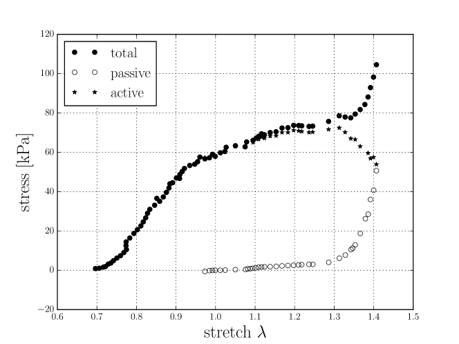
In order to model the activation of muscle tissue, a parameter can be introduced in the hyperelastic energy, such as in equation (2). We will now present two different ways of including the activation parameter in the same strain energy function; both of them aim to reproduce the active data of Figure 1.

Following the model by Ehret, Böl and Itskov [6], we describe the passive behavior of the skeletal muscle tissue as a transversely isotropic hyperelastic incompressible material. By frame-indifference, the passive strain energy density depends only on the right Cauchy-Green tensor $\mathbf{C}={\mathbf{F}}^{T}{\mathbf{F}}$ and is assumed to be

$$W_{p}({\mathbf{C}})=\frac{\mu}{4}\left\{\frac{1}{\alpha}\left[e^{\alpha({I}_{p}-1)}-1\right]+\frac{1}{\beta}\left[e^{\beta(K_{p}-1)}-1\right]\right\},\quad\det\mathbf{C}=1,$$ (4)

where

$${I}_{p}=\frac{w_{0}}{3}\operatorname{\rm tr}({\mathbf{C}})+(1-w_{0})\operatorname{\rm tr}({\mathbf{C}}{\mathbf{M}}),\ \ K_{p}=\frac{w_{0}}{3}\operatorname{\rm tr}({{\mathbf{C}}^{-1}})+(1-w_{0})\operatorname{\rm tr}({\mathbf{C}}^{-1}\mathbf{M}).$$

The tensor $\mathbf{M}=\mathbf{m}\otimes\mathbf{m}$ is called structural tensor, $\mathbf{m}$ being the orientation of the fibers. The incompressibility constraint $\det\mathbf{C}=1$ is due to the large amount of water contained in the skeletal muscle tissue. The material parameters $\alpha,\beta,w_{0}$ and $\mu$ are related to the passive proprieties of the muscle (in particular, $w_{0}$ measures the amount of anisotropy of the material).

In the following, we want to modify the passive model in order to account for the activation. Hence it is useful to introduce a constitutive assumption for $P_{act}$ , which is the active part of the stress given in Figure 1. As in [6], we assume that

$$P_{act}(\lambda)=\left\{\begin{aligned} &P_{opt}\frac{\lambda_{min}-\lambda}{\lambda_{min}-\lambda_{opt}}e^{\frac{(2\lambda_{min}-\lambda-\lambda_{opt})(\lambda-\lambda_{opt})}{2(\lambda_{min}-\lambda_{opt})^{2}}}&\text{if $\lambda>\lambda_{min}$},\\[4.30554pt] &0&\text{otherwise}.\end{aligned}\right.$$ (5)

The values of the material parameters, which have been obtained in [6] by least squares optimization using the experimental data, are given in Table 1. Notice that the value of $P_{opt}$ takes into account some information at the mesoscale level, such as the number of activated motor units and the interstimulus interval; in our model, $P_{opt}$ describes the maximal activation, which is reached in the tetanized case.

Table 1: Material parameters.

$\mu$ [kPa]	$\alpha$ [-]	$\beta$ [-]	$w_{0}$ [-]	$\lambda_{min}$ [-]	$\lambda_{opt}$ [-]	$P_{opt}$ [kPa]
0.1599	19.69	1.190	0.7388	0.682	1.192	73.52

3.1 First activation model: modification of the generalized invariant $I_{p}$

A simple way to model the activation is proposed in [6]. There, a parameter $\gamma\geq 0$ is introduced which adjusts the generalized invariant $I_{p}$:

$$\widetilde{I}=I_{p}+\gamma\operatorname{\rm tr}({\mathbf{C}}{\mathbf{M}})=\frac{w_{0}}{3}\operatorname{\rm tr}({\mathbf{C}})+(1-w_{0}+\gamma)\operatorname{\rm tr}({\mathbf{C}}{\mathbf{M}}).$$

In fact, the parameter $\gamma$ increases the amount of elastic energy during an elongation in the direction of the fibers. Then the total strain energy density becomes

$$W({\mathbf{C}},\gamma)=\frac{\mu}{4}\left\{\frac{1}{\alpha}\left[e^{\alpha(\widetilde{I}-1)}-1\right]+\frac{1}{\beta}\left[e^{\beta(K_{p}-1)}-1\right]\right\},\quad\det\mathbf{C}=1.$$ (6)

The stress evaluated on a uniaxial deformation along the fibers should fit the total stress of the experimental data reported in Figure 1; it turns out that $\gamma$ cannot be constant and it has to be considered as a function of the deformation. In order to choose a suitable model for the active parameter $\gamma(\mathbf{F})$, let us consider a uniaxial deformation of stretch $\lambda$ along the fiber direction $\mathbf{m}=\mathbf{e}_{1}$ in the transversely isotropic incompressible case:

$$\mathbf{F}=\begin{pmatrix}\lambda&0&0\\ 0&\frac{1}{\sqrt{\lambda}}&0\\ 0&0&\frac{1}{\sqrt{\lambda}}\end{pmatrix}.$$

Then the elastic energy density writes

$$W(\lambda,\gamma(\lambda))=\frac{\mu}{4}\left\{\frac{1}{\alpha}\left[e^{\alpha(\widetilde{I}(\lambda,\gamma(\lambda))-1)}-1\right]+\frac{1}{\beta}\left[e^{\beta(K_{p}(\lambda)-1)}-1\right]\right\}$$ (7)

with

$$\widetilde{I}(\lambda,\gamma(\lambda))=\frac{w_{0}}{3}\left({\lambda^{2}}+\frac{2}{\lambda}\right)+(1-w_{0}+\gamma(\lambda)){\lambda^{2}}=I_{p}(\lambda)+\gamma(\lambda)\lambda^{2},$$ (8)

$$K_{p}(\lambda)=\frac{w_{0}}{3}\left(\frac{1}{\lambda^{2}}+2\lambda\right)+\frac{1-w_{0}}{\lambda^{2}}.$$ (9)

Using (3), the total stress $P_{tot}$ and the passive stress $P_{pas}$ are given by

$$P_{tot}(\lambda,\gamma(\lambda))=\frac{\partial W}{\partial\lambda}(\lambda,\gamma(\lambda))+\frac{\partial W}{\partial\gamma}(\lambda,\gamma(\lambda))\gamma^{\prime}(\lambda),$$ (10)

$${P}_{pas}(\lambda)=\frac{\partial W}{\partial\lambda}(\lambda,0).$$ (11)

Hence, in order to fit the experimental data of the total stress, $\gamma$ has to solve the equation

$${P}_{tot}(\lambda,\gamma(\lambda))={P}_{pas}(\lambda)+{P}_{act}(\lambda),$$ (12)

which leads to the Cauchy problem

$$\left\{\begin{aligned} &\frac{\partial W}{\partial\lambda}(\lambda,\gamma(\lambda))+\frac{\partial W}{\partial\gamma}(\lambda,\gamma(\lambda))\gamma^{\prime}(\lambda)=P_{pas}(\lambda)+P_{act}(\lambda),\\[4.30554pt] &\gamma(\lambda_{min})=0.\end{aligned}\right.$$ (13)

The condition $\gamma(\lambda_{min})=0$ comes from the expression of $P_{act}$ in (5), i.e. we assume that the activation begins after $\lambda_{min}$.

We note that (13) can be explicitly integrated, so that $\gamma$ can be found by solving the equation

$$W(\lambda,\gamma(\lambda))=W(\lambda,0)+S_{act}(\lambda),$$ (14)

where

$$S_{act}(\lambda)=\left\{\begin{aligned} &\int_{\lambda_{min}}^{\lambda}P_{act}(\xi)d\xi&\text{if $\lambda>\lambda_{min}$},\\[4.30554pt] &0&\text{otherwise},\end{aligned}\right.$$ (15)

and

$$\int_{\lambda_{min}}^{\lambda}P_{act}(\xi)d\xi=P_{opt}(\lambda_{min}-\lambda_{opt})\left[e^{\frac{(2\lambda_{min}-\lambda-\lambda_{opt})(\lambda-\lambda_{opt})}{2(\lambda_{min}-\lambda_{opt})^{2}}}-e^{\frac{1}{2}}\right].$$ (16)

The solution of equation (14) is given by

$$\gamma(\lambda)=\frac{1}{\alpha\lambda^{2}}\ln{\left\{1+\frac{4\alpha}{\mu}S_{act}(\lambda)e^{\left[1-\frac{w_{0}}{3}\left(\lambda^{2}+\frac{2}{\lambda}\right)-(1-w_{0})\lambda^{2}\right]}\right\}}$$ (17)

and is represented in Figure 2.

Figure 2: The behavior of the activation parameter $\gamma(\lambda)$ give in (17).

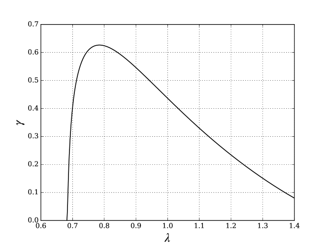
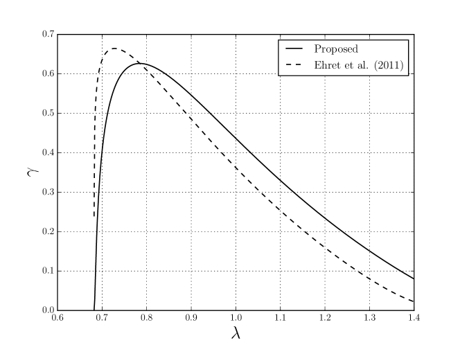
In the Appendix we will briefly comment the function $\gamma(\lambda)$ given in [6], which is different from (17). Indeed, in the computation of $P_{tot}$ in (10) we took into account that $\gamma$ has to depend on the stretch $\lambda$, while in [6] the derivative of the energy is computed as if $\gamma$ be a constant.

It is interesting to perform a numerical simulation for a general deformation. In that case, the stretch of the fibers $\lambda$ is given by the quantity

$$I_{4}=\sqrt{\operatorname{\rm tr}({\mathbf{C}}{\mathbf{M}})},$$

so that the energy density of the hyperelastic active skeletal muscle tissue is

$$W(\mathbf{C},\gamma(I_{4})),$$

where $W$ and $\gamma$ are given in (6) and (17), respectively. Taking into account that $\frac{\partial I_{4}}{\partial\mathbf{C}}=\mathbf{M}$, the expression of the stress becomes

$${\mathbf{P}}=2\mathbf{F}\frac{\partial W}{\partial\mathbf{C}}(\mathbf{C},\gamma(I_{4}))+2\frac{\partial W}{\partial\gamma}(\mathbf{C},\gamma(I_{4}))\,\frac{\partial\gamma}{\partial I_{4}}(I_{4})\,\mathbf{F}\mathbf{M}-p\mathbf{F}^{-T},$$

where $p$ is a Lagrange multiplier associated with the hydrostatic pressure which results from the incompressibility constraint $\det\mathbf{C}=1$.

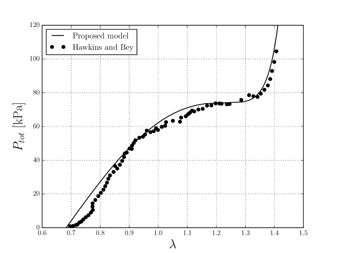
We simulate numerically a uniaxial deformation of a cylindrical slab of tissue, along the axis of the cylinder. We assume radial symmetry, so that the computational mesh reduces to a rectangle. Concerning the boundary conditions, the bases of the cylinder are kept perpendicular to the axial direction. Moreover, a basis of the cylinder is fixed and a load is applied to the other. The finite element simulation is performed using the open source project FEniCS [16], a collection of numerical software, supported by a set of novel algorithms and techniques, aimed at the automated solution of differential equations. In Figure 3 we show the stress-stretch relation obtained numerically, which fits the experimental data quite well.

Figure 3: Stress-stretch relation obtained using (17).

3.2 Second activation model: the active strain approach

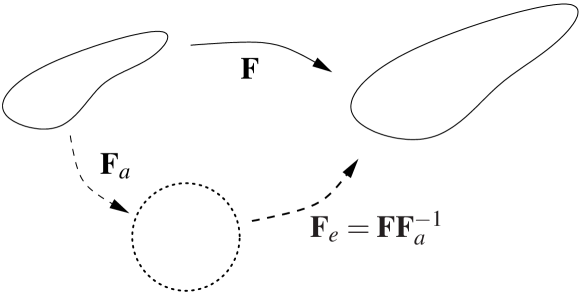
A more interesting way of modeling activation through a parameter is by means of active strain. Actually, the activation model considered in the previous section is halfway between active strain and active stress, which are the two main paths followed in the literature (for a review see [17]). The so called active stress method adds an extra contribution to the stress, accounting for activation (see for example [18, 19, 11]). On the other hand, the active strain approach assumes that only a part of the deformation gradient is responsible for storing the elastic energy, although the form of the strain energy function does not change. Similarly to the Kröner-Lee decomposition of finite plasticity [20], the deformation gradient is written as ${\mathbf{F}}={\mathbf{F}}_{e}{\mathbf{F}}_{a}$, where ${\mathbf{F}}_{e}$ is the elastic part and ${\mathbf{F}}_{a}$ describes the active contribution (see Figure 4). The tensor $\mathbf{F}_{a}$, which needs not be the gradient of some displacement, has a clear biological interpretation, since it is related to the sliding movement of the filaments in the sarcomeres, which is the main mechanism of contraction at the mesoscale. This method was first proposed by Taber and Perucchio [21] for the activation of the cardiac tissue, and it is detailed in [22] for soft living tissues. In [9] the active strain approach has been specifically applied to skeletal muscle tissue.

Figure 4: Pictorial view of the Kröner-Lee decomposition in the active strain approach.

Given a passive strain energy density $W_{p}$, the hyperelastic energy density of the activated material is given by

$${W}({\mathbf{C}},\mathbf{F}_{a})=(\det{\mathbf{F}}_{a})W_{p}({\mathbf{C}}_{e}),\quad\mathbf{C}_{e}={\mathbf{F}}^{-T}_{a}{\mathbf{C}}{\mathbf{F}}_{a}^{-1},$$

where the active strain ${\mathbf{F}}_{a}$ has to be constitutively prescribed as a function of the deformation gradient.

Let us consider the same passive strain energy density function given in (4) and choose the incompressible activation as

$${\mathbf{F}}_{a}(I_{4})=(1-\gamma(I_{4})){\mathbf{m}}\otimes{\mathbf{m}}+\frac{1}{\sqrt{1-\gamma(I_{4})}}({\mathbf{I}}-{\mathbf{m}}\otimes{\mathbf{m}}),\quad I_{4}=\sqrt{\operatorname{\rm tr}(\mathbf{C}\mathbf{M})},$$ (18)

where $0\leq\gamma<1$ represents the relative contraction of activated fibers ($\gamma=0$ meaning no contraction). Since $\det\mathbf{F}_{a}=1$, the modified strain energy density becomes

$${W}({\mathbf{C}},\gamma(I_{4}))=W_{p}({\mathbf{C}}_{e})=\frac{\mu}{4}\left\{\frac{1}{\alpha}\left[e^{\alpha(I_{e}-1)}-1\right]+\frac{1}{\beta}\left[e^{\beta(K_{e}-1)}-1\right]\right\},$$ (19)

where $\det\mathbf{C}=1$ and

$$I_{e}=\frac{w_{0}}{3}\operatorname{\rm tr}({\mathbf{C}}_{e})+(1-w_{0})\operatorname{\rm tr}({\mathbf{C}}_{e}{\mathbf{M}}),$$

$$K_{e}=\frac{w_{0}}{3}\operatorname{\rm tr}({{{\mathbf{C}}_{e}}^{-1}})+(1-w_{0})\operatorname{\rm tr}({{\mathbf{C}}_{e}}^{-1}{\mathbf{M}}).$$

As in Section 3.1, the parameter $\gamma$ has to be calibrated in order to obtain the active curve given in (5). Let us consider a uniaxial incompressible tension along the fiber direction ${\mathbf{m}}={\mathbf{e}}_{1}$, so that

$$\mathbf{C}_{e}=\begin{pmatrix}\frac{\lambda^{2}}{(1-\gamma(\lambda))^{2}}&0&0\\ 0&\frac{1-\gamma(\lambda)}{\lambda}&0\\ 0&0&\frac{1-\gamma(\lambda)}{\lambda}\end{pmatrix}.$$

Then the Cauchy problem (13) reduces again to equation (14) which, after some trivial simplifications, writes

$$\frac{1}{\alpha}e^{\alpha({I}_{e}(\lambda,\gamma(\lambda))-1)}+\frac{1}{\beta}e^{\beta(K_{e}(\lambda,\gamma(\lambda))-1)}=\frac{1}{\alpha}e^{\alpha({I}_{p}(\lambda)-1)}+\frac{1}{\beta}e^{\beta(K_{p}(\lambda)-1)}+\frac{4}{\mu}S_{act}(\lambda),$$ (20)

where

$$I_{e}(\lambda,\gamma(\lambda))=\frac{w_{0}}{3}\left[\frac{\lambda^{2}}{(1-\gamma(\lambda))^{2}}+\frac{2(1-\gamma(\lambda))}{\lambda}\right]+(1-w_{0})\frac{\lambda^{2}}{(1-\gamma(\lambda))^{2}},$$

$$K_{e}(\lambda,\gamma(\lambda))=\frac{w_{0}}{3}\left[\frac{(1-\gamma(\lambda))^{2}}{\lambda^{2}}+2\frac{\lambda}{1-\gamma(\lambda)}\right]+(1-w_{0})\frac{(1-\gamma(\lambda))^{2}}{\lambda^{2}},$$

$$I_{p}(\lambda)=I_{e}(\lambda,0),\quad K_{p}(\lambda)=K_{e}(\lambda,0).$$

Differently from the previous model, equation (20) cannot be explicitly solved, because the dependence of $W$ on $\gamma$ is much more complicated than before. However, one can employ standard numerical methods in order to find the solution. Figure 5, which is obtained by a bisection method, shows the solution $\gamma$ as a function of $\lambda$.

Figure 5: Numerical solution of equation (20).

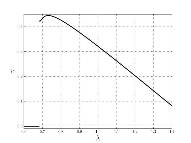
The behavior of the solution is quite similar to that shown in Figure 2, in the sense that it has a maximum point and then decreases to 0 for large $\lambda$. However, in this case $\gamma(\lambda)$ is discontinuous in $\lambda_{min}=0.682$.

In order to perform a finite element simulation, it is convenient to have an explicit function $\gamma(\lambda)$. A possible strategy is to choose a suitable form for $\gamma$ and to fit this expression to the data. Using a polynomial of degree 5 and running the simulation as in the previous section, we obtain Figure 6. As one can see, the numerical results describe quite well the experimental data.

Figure 6: Stress-stretch relation obtained using the active strain approach.

4 Concluding remarks

We analyzed the behavior of hyperelastic materials depending on a strain-dependent internal parameter $\gamma$. The parameter is introduced in the strain energy density function in order to capture some real phenomena such as growth and activation of biological tissues. In the fitting of experimental data, it is necessary to relate the internal parameter with the deformation gradient: in that case, if the material is supposed to be hyperelastic, a further term appears in the stress tensor, due to the derivative of $\gamma$ with respect to the deformation gradient. The present paper underlines the importance of considering such a term in order to get the proper behavior of the stress.

To this aim, we focused our attention on active skeletal muscle tissue, where it is often useful to consider an internal parameter describing the activation state of the muscle in its tetanized state. Starting from [6, 9], two different ways of including $\gamma$ in the hyperelastic energy are presented. First, activation is described following the approach used in [6] and the corresponding hyperelastic energy is found. Second, the active strain approach studied in [9] is used. In both cases, $\gamma$ is given as the solution of an equation which relates the passive and active strain energy functions. We remark that the first approach is not customary in the literature, while the active strain method seems to be closer to the biological meaning of activation. However, the simplicity of the first method allows to find an explicit function for $\gamma$, differently from the active strain case.

Notice that, once the dependence of $\gamma$ on the deformation has been taken into account, the hyperelastic energy of the active material can lose some of the mathematical properties of the passive one: for instance, if the latter is polyconvex, as in the case of (4), the former can even be not rank-1 convex. A future development will be a study of the properties of the active material depending on the form of the activation function $\gamma$ and the passive energy.

Appendix A Comparison with the activation parameter in [6]

The aim of this Appendix is to point out the differences between the activation parameter $\gamma(\lambda)$ computed in Section 3.1 and the results of [6, Sect. 3.1].

Let us consider again a uniaxial deformation along the fibers and the elastic energy (7). If one computes the derivative of the energy as if $\gamma$ were a constant, it follows that

$${P}_{tot}(\lambda,\gamma)=\frac{\partial W}{\partial\lambda}(\lambda,\gamma)=\frac{\mu}{4}\left[\frac{\partial\widetilde{I}}{\partial\lambda}(\lambda,\gamma)\,e^{\alpha(\widetilde{I}(\lambda,\gamma)-1)}+\frac{\partial K_{p}}{\partial\lambda}(\lambda)\,e^{\beta(K_{p}(\lambda)-1)}\right],$$ (21)

where $\widetilde{I}$ and $K_{p}$ are given in (8)-(9) and

$$\frac{\partial\widetilde{I}}{\partial\lambda}(\lambda,\gamma)=2\frac{w_{0}}{3}\left({\lambda}-\frac{1}{\lambda^{2}}\right)+2(1-w_{0}+\gamma){\lambda}=I_{p}^{\prime}(\lambda)+2\gamma\lambda,$$

$$\frac{\partial K_{p}}{\partial\lambda}(\lambda)=2\frac{w_{0}}{3}\left(-\frac{1}{\lambda^{3}}+1\right)-2(1-w_{0})\frac{1}{\lambda^{3}}.$$

The passive part of the stress is given by ${P}_{pas}(\lambda)={P}_{tot}(\lambda,0)$ and, in order to fit the experimental data of the total stress, $\gamma$ has to solve the equation

$${P}_{tot}(\lambda,\gamma(\lambda))={P}_{pas}(\lambda)+{P}_{act}(\lambda),$$

where $P_{act}$ is again given by (5). Such an equation is not so easy to solve in $\gamma$, since it is of the form

$$\Big{(}I^{\prime}_{p}(\lambda)+2\lambda\gamma\Big{)}e^{\alpha\lambda^{2}\gamma}=f(\lambda),$$

where $f(\lambda)$ is a given function of $\lambda$. However, after some calculations the solution writes

$$\gamma(\lambda)=\left\{\begin{aligned} &\frac{W_{0}(x^{*}(\lambda))}{\alpha\lambda^{2}}-\frac{I_{p}^{\prime}(\lambda)}{2\lambda}&&\text{if $\lambda>\lambda_{min}$},\\[4.30554pt] &0&&\text{otherwise},\end{aligned}\right.$$ (22)

where $W_{0}$ is the Lambert W-function, which is the inverse of $xe^{x}$, and

$$x^{*}(\lambda)=P_{act}(\lambda)\frac{2\alpha\lambda}{\mu}e^{\frac{\alpha}{2}(2-2I_{p}(\lambda)+\lambda I_{p}^{\prime}(\lambda))}+\frac{\alpha}{2}\lambda I_{p}^{\prime}(\lambda)e^{\frac{\alpha}{2}\lambda I_{p}^{\prime}(\lambda)}.$$

As one can see, even if the internal parameter $\gamma$ is a function of $\lambda$, the stress (21) has been computed assuming that $\gamma$ is independent of the strain. In particular, the stress (21) does not come from the hyperelastic energy $W(\lambda,\gamma(\lambda))$. Moreover, from a mathematical viewpoint the expression of $\gamma$ in (17) is much simpler than the one given in (22).

The trend of $\gamma(\lambda)$ is showed in Figure 7 in comparison to the one obtained in Section 3.1.

Figure 7: Comparison between the behavior of $\gamma(\lambda)$ in (17) (solid line) and the one in (22) (dashed line).

References

- [1] G. Chagnon, M. Rebouah, and D. Favier. Hyperelastic Energy Densities for Soft Biological Tissues: A Review. Journal of Elasticity, 120(2):129–160, 2015.
- [2] K. A. Lazopoulos and R. W. Ogden. Nonlinear Elasticity Theory with Discontinuous Internal Variables. Mathematics and Mechanics of Solids, 3(1):29–51, 1998.
- [3] R. W. Ogden and D. G. Roxburgh. A pseudo–elastic model for the Mullins effect in filled rubber. Proceedings of the Royal Society of London A: Mathematical, Physical and Engineering Sciences, 455(1988):2861–2877, 1999.
- [4] K.R. Rajagopal and A.S. Wineman. A constitutive equation for nonlinear solids which undergo deformation induced microstructural changes. International Journal of Plasticity, 8(4):385 – 395, 1992.
- [5] Markus Böl, Roman Weikert, and Christine Weichert. A coupled electromechanical model for the excitation-dependent contraction of skeletal muscle. Journal of the Mechanical Behavior of Biomedical Materials, 4(7):1299–1310, 2011.
- [6] Alexander E. Ehret, Markus Böl, and Mikhail Itskov. A continuum constitutive model for the active behaviour of skeletal muscle. Journal of the Mechanics and Physics of Solids, 59(3):625–636, 2011.
- [7] B. Hernández-Gascón, J. Grasa, B. Calvo, and J.F. Rodríguez. A 3D electro-mechanical continuum model for simulating skeletal muscle contraction. Journal of Theoretical Biology, 335:108–118, 2013.
- [8] J. Weickenmeier, M. Itskov, E. Mazza, and M. Jabareen. A physically motivated constitutive model for 3D numerical simulation of skeletal muscles. International Journal for Numerical Methods in Biomedical Engineering, 30(5):545–562, 2014.
- [9] Giulia Giantesio and Alessandro Musesti. A continuum model of skeletal muscle tissue with loss of activation. In Alf Gerisch, Raimondo Penta, and J. Lang, editors, Multiscale Models in Mechano and Tumor Biology: Modeling, Homogenization, and Applications, Lecture Notes in Computational Science and Engineering. Springer, in press.
- [10] Babak Sharifimajd and Jonas Stålhand. A continuum model for skeletal muscle contraction at homogeneous finite deformations. Biomechanics and Modeling in Mechanobiology, 12(5):965–973, 2013.
- [11] Thomas Heidlauf and Oliver Röhrle. A multiscale chemo-electro-mechanical skeletal muscle model to analyze muscle contraction and force generation for different muscle fiber arrangements. Frontiers in Physiology, 5:498, 2014.
- [12] Cornelius O. Horgan, Ray W. Ogden, and Giuseppe Saccomandi. A theory of stress softening of elastomers based on finite chain extensibility. Proceedings of the Royal Society of London A: Mathematical, Physical and Engineering Sciences, 460(2046):1737–1754, 2004.
- [13] C. Paetsch, B.A. Trimmer, and A. Dorfmann. A constitutive model for active-passive transition of muscle fibers. International Journal of Non-Linear Mechanics, 47(2):377–387, 2012.
- [14] Carol A. Oatis. Kinesiology. The Mechanics and Pathomechanics of Human Movement. Lippincott Williams & Wilkins, 2nd edition, 2009.
- [15] D Hawkins and M. Bey. A Comprehensive Approach for Studying Muscle-Tendon Mechanics. ASME Journal of Biomechanical Engineering, 116:51–55, 1994.
- [16] Martin Alnæs, Jan Blechta, Johan Hake, August Johansson, Benjamin Kehlet, Anders Logg, Chris Richardson, Johannes Ring, Marie Rognes, and Garth Wells. The FEniCS Project Version 1.5. Archive of Numerical Software, 3(100):9–23, 2015.
- [17] D. Ambrosi and S. Pezzuto. Active Stress vs. Active Strain in Mechanobiology: Constitutive Issues. Journal of Elasticity, 107:199–212, 2012.
- [18] J.a.C. Martins, E.B. Pires, R. Salvado, and P.B. Dinis. A numerical model of passive and active behavior of skeletal muscles. Computer Methods in Applied Mechanics and Engineering, 151(3-4):419–433, 1998.
- [19] Silvia S Blemker, Peter M Pinsky, and Scott L Delp. A 3D model of muscle reveals the causes of nonuniform strains in the biceps brachii. Journal of biomechanics, 38(4):657–65, 2005.
- [20] Antonıo DiCarlo and Sara Quiligotti. Growth and balance. Mechanics Research Communications, 29(6):449–456, 2002.
- [21] Larry A. Taber and Renato Perucchio. Modeling heart development. Journal of Elasticity, 61(1):165–197, 2000.
- [22] Paola Nardinocchi and Luciano Teresi. On the Active Response of Soft Living Tissues. Journal of Elasticity, 88(1):27–39, 2007.