Additional authors: Matthias Schubert (LMU Munich, Oettingenstraße 67, 80583 Munich, Germany) schubert@dbs.ifi.lmu.de)
Scenic Routes Now: Efficiently Solving the Time-Dependent Arc Orienteering Problem
This paper extends the Arc Orienteering Problem (AOP) to large road networks with time-dependent travel times and time-dependent value gain, termed Twofold Time-Dependent AOP or 2TD-AOP for short. In its original definition, the NP-hard Orienteering Problem (OP) asks to find a path from a source to a destination maximizing the accumulated value while not exceeding a cost budget. Variations of the OP and AOP have many practical applications such as mobile crowdsourcing tasks (e.g., repairing and maintenance or dispatching field workers), diverse logistics problems (e.g., crowd control or controlling wildfires) as well as several tourist guidance problems (e.g., generating trip recommendations or navigating through theme parks). In the proposed 2TD-AOP, travel times and value functions are assumed to be time-dependent. The dynamic values model, for instance, varying rewards in crowdsourcing tasks or varying urgency levels in damage control tasks. We discuss this novel problem, prove the benefit of time-dependence empirically and present an efficient approximative solution, optimized for fast response systems. Our approach is the first time-dependent variant of the AOP to be evaluated on a large scale, fine-grained, real-world road network. We show that optimal solutions are infeasible and solutions to the static problem are often invalid. We propose an approximate dynamic programming solution which produces valid paths and is orders of magnitude faster than any optimal solution.††⋆These authors contributed equally to this work.
1 Introduction
Not long ago, finding the shortest or fastest path in road networks was the core challenge of route planning. Nowadays, challenges are manifold – due to the abundance of sensor data, due to the existence of increasingly complex traffic models and due to the demand for efficient yet convenient solutions. Modern navigation systems often take multiple, sometimes time-dependent, cost criteria into account and solve complex queries in order to increase driver convenience and traffic efficiency. In view of this progress, we propose a novel query with multiple applications. As an extension to the family of Orienteering Problems, we present the Twofold Time-Dependent Arc Orienteering Problem (2TD-AOP).
In its original formulation [OriginalPaper-87], the Orienteering Problem (OP) requires to find a path from a given source to a given destination abiding by a given cost budget but maximizing the value collected along the way. In most cases, the cost function corresponds to the travel time within the given network. The problem may for instance occur in the field of spatial crowdsourcing [CSMTA-GeocrowdEnablingQueryAnsweringWithSpatialCrowdsourcing12SHAHABI, CS-Chen-VLDB-15, CS-Shahabi-ACM-15] where individuals complete advertised tasks in order to collect rewards. A recent popular example of this is the augmented reality game Pokémon Go. A worker who is willing to complete crowdsourced tasks will want to maximize the collected rewards within his chosen time frame. The OP combines the NP-hard Knapsack and Traveling Salesman Problems, hence is NP-hard itself. Numerous variations of the problem have been proposed, for instance, extending it to multiple workers (Team Orienteering Problem) [OP-Survey-Vansteenwegen-16] or restricting the collectable values to certain time windows ((Team) Orienteering Problem with Time Windows) [TTDP-Survey-Gavalas-14]. Another variation is the Arc Orienteering Problem (AOP) [AOP-Survey-ArchettiSperanza-13]. In the OP, the value is associated with the vertices of the graph, whereas in the AOP, it is associated with the arcs. Thus, the OP intuitively corresponds to logistic or crowdsourcing tasks, where the value is collected at particular points. The AOP, on the other hand, corresponds to tasks where the value is collected “along the way”. Examples of such tasks are the routes of firefighting planes or the planning of scenic bike trips [AOP-GRASP-PlanningOfCycleTripsInEastFlanders-VANSTEENWEGEN-OMEGA10].
Until recently, the AOP has only been answered for networks with static travel times. However, assuming static costs is not reasonable for most real-world scenarios. For road networks, the significance of time-dependence was empirically proven in [TD-CaseForTimeDepRoadNetworks-FoundationPaper-DEMIR-SHAHABI-GIS10] and substantiated by the incorporation into many navigation services such as Waze111waze.com. In a recent study, Verbeeck et. al [TDOP-YING-AntColony-DriveSpeedModel-FastSolutionToTDOP-OR14-VANSTEENWEGEN] first introduced time-dependent travel times but the values have been assumed to be static. In this paper, we propose to incorporate time-dependent values in addition to time-dependent travel times, introducing the 2TD-AOP. As will be shown, results benefit greatly from time-dependent values which model the varying benefit for different times. Without loss of generality, we restrict ourselves to the application of scenic route planning. In this use case, a view of the sea might only be worthwhile during day, whereas a view of the skyline might be particularly worthwhile at night. Thus, the value of a coastline road is high during the day but low at night, while a road passing through downtown may have the opposite values. Other use cases include the aforementioned firefighting planes, collecting street view data or gathering Pokémon Go items.
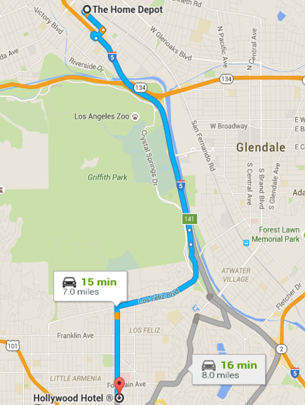
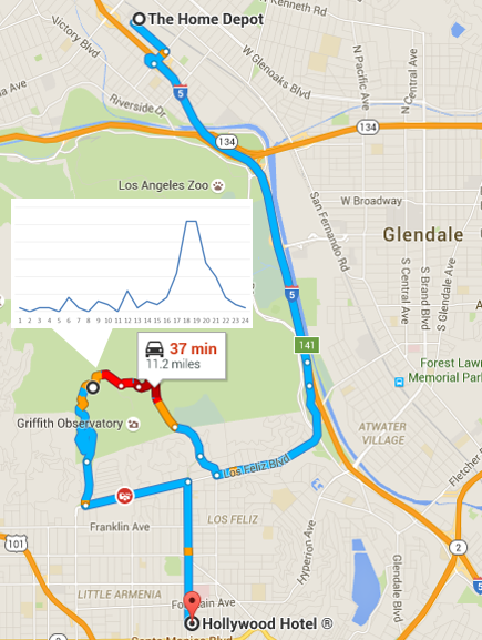
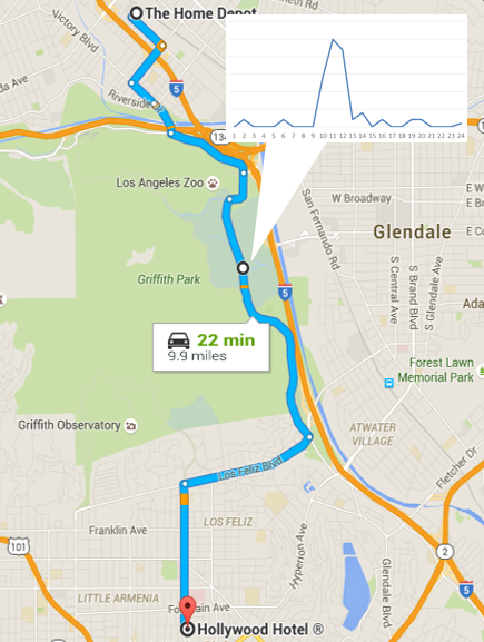
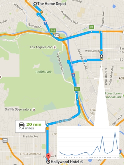
Consider the example given in Figure 1 which shows different result paths for a scenic path query with the same source and destination. Figure 1(a) shows the time-dependent fastest path according to our algorithm for two departure times. While the path is the same at 11 am and 6 pm, the travel times are not the same (15 and 20 minutes, respectively). In this example, the fastest path does not pass through particularly scenic areas, according to the crowdsourced data set. The other paths pass through such areas, and for particular scenic parts of the respective paths, the hourly value distributions are highlighted. At first glance it is evident that the value functions show great variance over the course of a day. If not allowing for time-dependent values, these functions are commonly averaged, evening out the significant peaks of the distribution.
Suppose a driver is willing to spend 25 minutes for his trip from Hollywood Hotel to the Home Depot north of Griffith Park. Employing an algorithm for the AOP in static networks[AOP-Ying-Shahabi-ACMGIS-15], we obtain the static scenic path displayed in Figure 1(b). The path was computed in a static network derived from our time-dependent network. The static travel time along an arc is set as the average of all travel times along this arc in the time-dependent network. The static scenicness values are derived analogously. The generated result path has a static travel time of 22 minutes which abides by the budget. However, the actual travel time might of course deviate in either direction. For a desired departure at 11 am, the time-dependent travel time coincides with the static time of 22 minutes, but for a desired departure at 6 pm, the time-dependent path takes 37 minutes. Thus, at 6 pm the result path clearly exceeds the budget and is therefore invalid. In a similar way, the averaged scenicness values can deviate from the time-dependent ones. While the static scenic path at 11 am does not exceed the budget, it is not optimal either. Griffith Observatory, which it passes along the way, is a popular sight but particularly scenic during sunset or in the evening. Instead, the best solution at 11 am is displayed in Figure 1(c). This time-dependent scenic path takes 20 minutes and passes a golf course, offering particularly nice views at daytime. The best solution at 6 pm is shown in Figure 1(d). This path takes 22 minutes and passes through central Glendale, a bustling area in the evening and at night.
Taking time-dependence into account when computing AOP paths is crucial. Not only result quality but also result validity depends on it. Our experiments show that every second static solution in a moderately complex settings is invalid. Users benefit considerably from time-dependent travel times as every 2TD-AOP path is valid. Furthermore, results are improved significantly when the values reflect time-dependence as well. Our experiments show that 2TD-AOP paths generate three to four times more value than static solutions. We therefore propose to employ value distribution models whenever possible.
Due to their NP-hardness, static variations of the OP and AOP are usually solved employing metaheuristics. Allowing for time-dependent travel times adds further complexity to the task. Slight modifications of valid solutions may invalidate them. For instance, when taking a minor detour at the beginning of the path, travel times for the rest of the path may change and exceed the budget. Additionally incorporating time-dependent values multiplies this effect. Taking a minor detour at the beginning of a path may result in a change of value and travel time. We propose to solve the 2TD-AOP with a novel dynamic programming approach which makes use of pruning techniques to limit the candidate set and reduce intermediate path computations.
To the best of our knowledge, no previous work has allowed for both travel times and values to be time-dependent. In addition to handling the increased complexity, we require fast response times. We focus on the practicality of the solution where fast response times are crucial and large road network are standard, for instance, in order to meet the requirements of a mobile application. In conclusion, the contributions of this paper are as follows:
-
1.
We motivate and introduce the 2TD-AOP, as a new graph-based routing problem and a Mixed Integer Programming formulation.
-
2.
We present an efficient approximate solution to the 2TD-AOP.
-
3.
We present experiments on a large-scale real-world road network. Our evaluation is the first of this dimension for any time-dependent AOP. We show the value of twofold time-dependence empirically and compare 2TD-AOP solutions to static solutions as well as to optimal results.
The remainder of this paper is organized as follows. In Section 2 we give an overview of research relevant to our work. In Section 3 the 2TD-AOP is formally defined and formulated as an Mixed Integer Programming. In Section 4 we lay the theoretical foundation for our algorithm which is described in Sections 5 and 6. Subsequently, our algorithm is evaluated in Section LABEL:sec:exp. A conclusion is provided in Section LABEL:sec:conclusion.
2 Related Work
We divide research relevant to this work into three groups. First, we review research on how to attain profit values from data in general and crowdsourced content in particular. Next, we briefly introduce related research from the database community such as the Trip Planning Query (TPQ). These problems have a similar field of application but are not congruent to the problem discussed in this paper. Finally, we present research on the family of OPs which mostly stems from the field of Operations Research. We give an overview of solutions to the static and time-dependent OP and AOP.
2.1 Attaining Value Functions
An important aspect of the OP/AOP is how to attain the value functions, in particular when aiming to solve a time-dependent instance. Most works from the field of Operations Research rely on specific bench mark data sets, some synthetic, others real. The authors of [AOP-GRASP-PlanningOfCycleTripsInEastFlanders-VANSTEENWEGEN-OMEGA10], for instance, evaluate their approach to cycle trip planning on real-world tourist data from Flanders, Belgium. The authors of [TDOP-MathematicalModelMetaheuristicsTDOP-Gunawan2014] use data from Chinese theme parks. Relying on specifically recorded data like the above has two major drawbacks. First, expert knowledge or an official mandate may be required to attain the data. Second, the data may not be available globally. As this approach usually lacks scalability, there exist advances to mine this knowledge from freely available data.
Crowdsourced data is a rich source of information. It is for instance used for general POI recommendation [TDOP-YING-PredOfCIKM14-ExploitingLargeScaleCheckInDataToRecommendTimeSensitiveRoutes-UrbComp12], for categorization [TDVCOP-TripPlannerPersTripPlanLeveragingHeterogenCrowdsourcedDigiFootprints-TITS14], for popularity estimation [POI-Preferences-Categories-GenMaxCover-PlanningTouristicToursWithTripBuilder-CIKM13], for determining opening hours or visiting times [TDOP-YING-Gowalla-CheckIns-MiningPlanningTimeAwareRoutesfromCheckInData-CIKM14], for determining duration of stay [POI-VisTimeFromFlickrPics-AutomaticConstructionOfTravelItinerariesFromSocialBreadcrumbs-YAHOO10] or for determining spatial connectivity [SSTD15-Knowledge]. The most common data sources for these purposes are Foursquare, Yelp, Twitter, Flickr222foursquare.com, yelp.com, twitter.com, flickr.com or the inoperative but oft-cited Gowalla. When interested in how to attain value functions from the raw data, we refer the reader to the respective works. In the context of this paper, we assume the values to be given. For our experimental evaluation, we rely on Flickr data, details are given in Section LABEL:sec:exp.
2.2 TPQ and Related Queries
The most related query in the database community is the TPQ [TPQ] (alternatively, Route Planning Query [MRPSRQ] or Route Search Query [LevKanSafSag09]). In this problem setting, the user specifies a different POI categories, e.g., “ATM”, “restaurant”, “florist”, “cinema”. The result of a TPQ is the fastest path from a given source to a given destination visiting exactly one instance of each resource. The TPQ is NP-hard because in the case that each category occurs exactly once, the TPQ degenerates to the Traveling Salesman Problem. There exist several variations, for instance introducing order constraints [OSR, InteractiveRouteSearchPresenceOrderConstraints] or modeling the fulfillment at a location probabilistically or time-dependent [FollowUpToKRoute, EDBT15-ResourceRoute, DelEfsVer11]. Solutions to this problem include full enumeration [DelEfsVer11], heuristics [MRPSRQ, OSR, DelEfsVer11], or backtracking and branch-and-bound approaches [EDBT15-ResourceRoute]. Partially time-dependent variations of these queries exist, however, most of the research pertains to static networks. Most importantly, albeit related, the problem settings of the OP/AOP and the TPQ are not congruent.
2.3 OP and AOP
Blueprint for the OP was the family of orienteering sports where efficient navigation from checkpoint to checkpoint is the goal [OriginalPaper-87]. Alternative names for the OP include the Selective Traveling Salesman Problem [OP-STSP] or the Traveling Salesman Problem with Profits [OP-TSPwithProfits]. The OP is executed on a graph whose arc weights represent traversal costs and whose vertices may yield certain value. Given a source, a destination and a cost budget, the output of an OP is the path with maximum value among all paths not exceeding the budget. In the variation referred to as AOP or Privatized Rural Postman Problem [AOP-PrivatizedRuralPostmanProblems], the profit is not assigned to vertices but to arcs, while the rest is as before. Extensive surveys on these problems and their numerous variants are given in [OP-Survey-Vansteenwegen-11, OP-Survey-Vansteenwegen-16, AOP-Survey-ArchettiSperanza-13] (or from the perspective of the related Tourist Trip Design Problem in [TTDP-Survey-Gavalas-14]).
Although NP-hard [OriginalPaper-87], exact solutions to the OP exist [OP-STSP, OP-Exact-Ramesh-91, OP-TSPwithProfits]. Most solutions, however, are approximative. While in older research specific heuristic approaches were proposed [OP-Heuristics-84, OP-Heuristic-Golden-88, OP-Heuristic-Chao-96], the trend shifted towards algorithms following particular meta-heuristics such as Tabu Search [OP-TabuSearch-Gendreau-98], Genetic Algorithms [OP-Genetic-Tasgitiren-01] or Ant Colony Algorithms [OP-AntColony-Liang-02]. This holds similarly for the AOP where exact algorithms [AOP-Exact, AOP-ILS-ExtensionOfAOPAndApplicationCycleTripPlanning-VANSTEENWEGEN-TR14] are rare but available. Generating approximative solutions is the standard approach [AOP-AppoximationAlgorithms-Gavalas-14], most effectively following the meta-heuristics Iterative Local Search (ILS) [AOP-ILS-ExtensionOfAOPAndApplicationCycleTripPlanning-VANSTEENWEGEN-TR14] and Greedy Randomized Adaptive Search Procedure (GRASP) [AOP-GRASP-PlanningOfCycleTripsInEastFlanders-VANSTEENWEGEN-OMEGA10, AOP-Ying-Shahabi-ACMGIS-15]. Recently, ILS and GRASP have been improved to solve the AOP on large scale real-world road networks in near-interactive time [AOP-Ying-Shahabi-ACMGIS-15].
Introduced in [TDOP-NPhardness-FirstApprox-Fomin-02], the OP with time-dependent (TD-OP) costs has gained attention recently [TDOP-MathematicalModelMetaheuristicsTDOP-Gunawan2014, TDTOPTW-Garcia-First-09, TDTOPTW-EfficientHeuristicsForTDTOPTW-13, TDOP-YING-AntColony-DriveSpeedModel-FastSolutionToTDOP-OR14-VANSTEENWEGEN, TDOP-ResearchOnTOPwithDynamicTT-Li-12]. Typical applications for the TD-OP include electronic tourist guides [TDTOPTW-Garcia-First-09, TDTOPTW-POI-PublicTransport-PersonalizedTouristRouteGen-10] or routing in theme parks [TDOP-MathematicalModelMetaheuristicsTDOP-Gunawan2014]. The time-dependent AOP (TD-AOP) as presented in [TDOP-YING-AntColony-DriveSpeedModel-FastSolutionToTDOP-OR14-VANSTEENWEGEN] is not directly linked to an application but a time-dependent extension of the authors’ cycle trip planning application [AOP-ILS-ExtensionOfAOPAndApplicationCycleTripPlanning-VANSTEENWEGEN-TR14] is imaginable.
The above works are all evaluated on small graphs (with the exception of [AOP-Ying-Shahabi-ACMGIS-15]) with no more than a couple of hundred vertices. Most arcs in these graphs connect two non-zero value vertices. For instance, in the theme park data set of [TDOP-MathematicalModelMetaheuristicsTDOP-Gunawan2014], vertices correspond to attractions and the arcs are fastest paths between them. The travel times and the values are derived from user data of the theme parks and their attractions. Similarly, [TDTOPTW-EfficientHeuristicsForTDTOPTW-13] and the demonstration paper [TDTOPTW-POI-PublicTransport-PersonalizedTouristRouteGen-10] are evaluated on data sets consisting of Points of Interest (POIs) and fastest paths connecting these POIs (by walking or by public transportation). When considering real-world road networks, this is not feasible. A moderate-sized network usually contains over one million vertices and two to three million arcs. In a time-dependent network, there usually exist numerous fastest paths from a given vertex to another, depending on the departure time. Hence, introducing shortcuts for precomputed fastest paths as in the approaches above is not possible. This is particularly the case, if the travel times are not statistically inferred but real-time, i.e., depending on live information, as is the case in the network of our evaluation.
The most closely related problem to the 2TD-AOP is the TD-AOP with time-dependent costs and static value. Verbeeck et. al recently proposed to solve this problem with an Ant Colony System algorithm [TDOP-YING-AntColony-DriveSpeedModel-FastSolutionToTDOP-OR14-VANSTEENWEGEN]. Evaluated on specific benchmark instances with at most 100 vertices, the proposed approach finds near-optimal to optimal solutions within an average runtime of one second. The complex solver has excessive time requirements (“often more than 100 hours” [TDOP-YING-AntColony-DriveSpeedModel-FastSolutionToTDOP-OR14-VANSTEENWEGEN]) to generate optimal solutions on these benchmark instances of the TD-AOP. In comparison, we increase complexity of the problem in two ways. First, by including time-dependent value functions 2TD-AOP adds another dimension of time-dependence to the problem. Second, we aim to solve the problem on large-scale real-world road networks with hundred thousands of vertices. Established solutions to related problems like the TD-AOP or the TD-OP rely on metaheuristics such as the Ant Colony System [TDOP-YING-AntColony-DriveSpeedModel-FastSolutionToTDOP-OR14-VANSTEENWEGEN], Iterative Local Search [AOP-ILS-ExtensionOfAOPAndApplicationCycleTripPlanning-VANSTEENWEGEN-TR14] or Greedy Randomized Adaptive Search Procedure [AOP-GRASP-PlanningOfCycleTripsInEastFlanders-VANSTEENWEGEN-OMEGA10, AOP-Ying-Shahabi-ACMGIS-15]). Instead, we propose a heuristic dynamic programming approach.
3 Problem Definition
We model the road network as a graph , where denotes the set of vertices (or nodes), denotes the set of directed arcs (or edges), and (with the same domains) denote the non-negative functions mapping each arc onto its respective value and the travel time, respectively
For the representation of the time-dependent travel time along an arc, we use a piecewise constant function with equal step width . In the following, we refer to the intervals where travel time is constant as time windows and denote the -th time window by , where for some maximum time window .
A consecutive set of arcs which visits no arc twice is called a path. A path from source to destination departing at is denoted by where is the source vertex and the destination vertex. In the remainder of this paper, we simplify notation for the sake of clarity. We omit the double indexes and denote a path by
For each query, we denote source and destination by and , respectively. The travel time of a path is defined as , where denotes the time of arrival at (and departure from) vertex . is dependent on the travel times along the preceding arcs and is defined iteratively:
The value of a path is defined as:
For a given source , destination , and departure time , we denote the set of all paths from to starting at by .
The input for the 2TD-AOP is a graph , a source vertex , a destination vertex , a departure time , and a time budget . When speaking of a query, we mean the set of these inputs. The optimal path to a 2TD-AOP query is the path maximizing the collected value among all feasible paths. Both notions are defined in the following.
Definition 1 (feasible path)
Given a query, we call any path departing from at and arriving at no later than (i.e., ) a feasible path.
Definition 2 (optimal path)
Given a query, among all feasible paths, we call one with maximum value an optimal path.
Extending the work in [OP-Survey-Vansteenwegen-11, TDOP-YING-AntColony-DriveSpeedModel-FastSolutionToTDOP-OR14-VANSTEENWEGEN], we give a mixed integer programming (MIP) formulation of the problem. We introduce the following two decision variables: is a binary decision variable which equals if the result path enters the arc in time window and if the arc is not traversed at all or entered in a different time window. is a continuous decision variable containing the time of departure at when entering the arc in time window . Again, it is if the arc is not traversed at all or entered in a different time window.
| (1a) | |||
| (1b) | |||
| (1c) | |||
| (1d) | |||
| (1e) | |||
| (1f) | |||
| (1g) | |||
| (1h) | |||
Equation 1a gives the objective function while Equation 1b gives the budget constraint. Note that due to the time-dependent nature of the problem, all time windows have to be taken into account when summing the collected value and cost. Remember, however, that is a binary decision variable which for each arc can at most once be equal to , as each vertex (and thereby also each arc) is at most visited once. This is expressed in Constraint 1. Constraint 1d ensures that the result path starts at the source and ends at the destination. Next, Constraint 1 ensures that the departure time at each arc is the departure time at its predecessor plus the travel time within the corresponding time window. Note that this condition implicitly forbids “waiting” at vertices. Finally, Constraints 1f and 1g determine the domain of the decision variables and Constraint 1h ensures that the path departs from the source at .
4 Solving the 2TD-AOP
In this section, we present terminology and insights essential to our solution of the 2TD-AOP.
Definition 3 (earliest arrival)
Given a graph , a source , a vertex , and a departure time , we define the earliest arrival (time) for reaching from when departing at , denoted by ( for short), as follows:
Definition 4 (latest departure)
Given a graph , a destination , a vertex , and a latest arrival time , we define the latest departure (time) for reaching from no later than , denoted by ( for short), as follows:
i.e., the latest departure time among all feasible paths w.r.t. , , and .
Definition 5 (forward-reachable)
Given a graph , a source , a departure time , and a time budget , we refer to the vertices reachable within the budget from (when departing at ) as forward-reachable vertices, denoted by (FWR for short if and are clear from context).
Definition 6 (backward-reachable)
Given a graph , a destination , a departure time , and a time budget , we refer to the vertices from which the destination can be reached within the budget when departing no earlier than as backward-reachable vertices, denoted by (BWR for short).
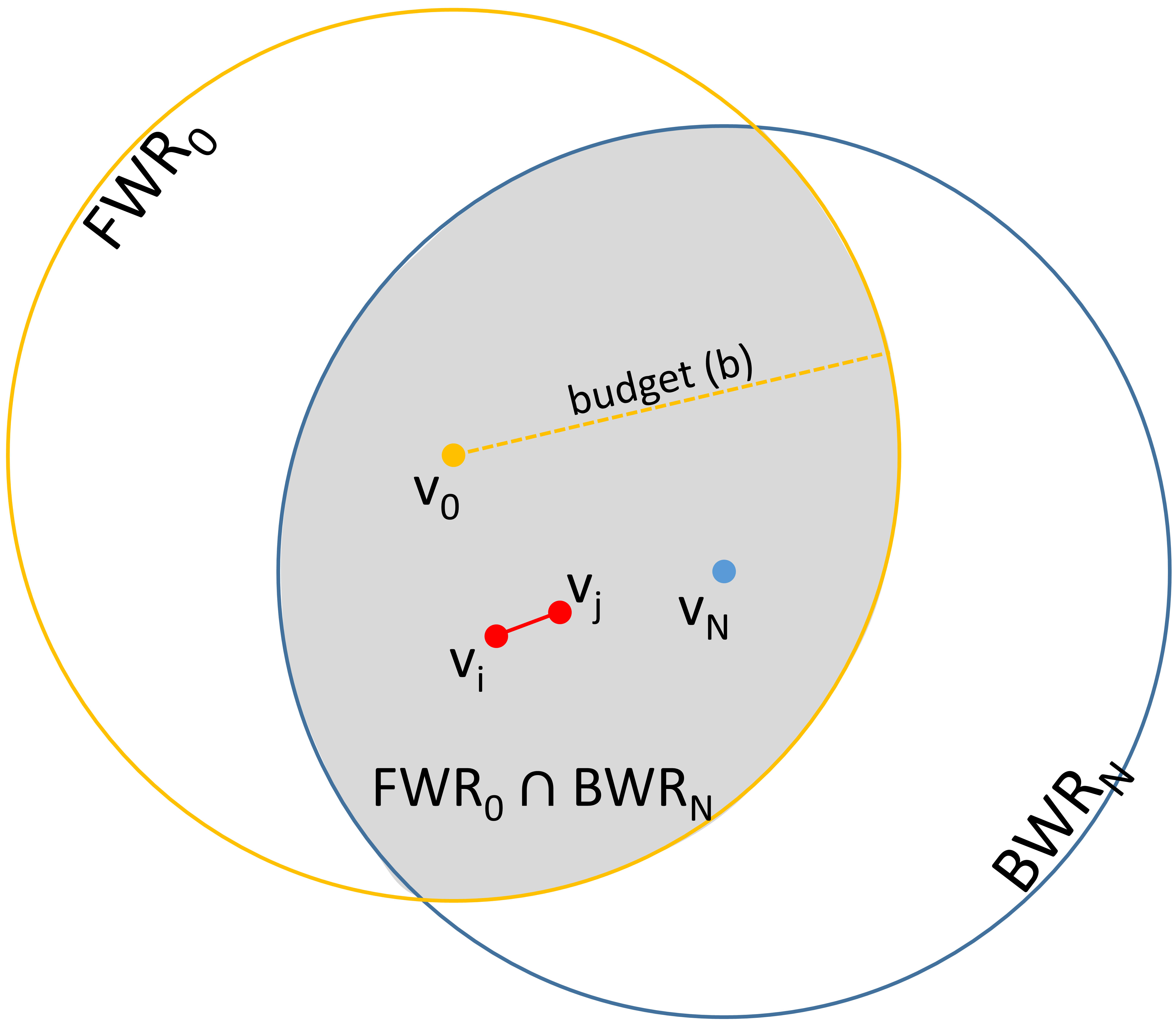
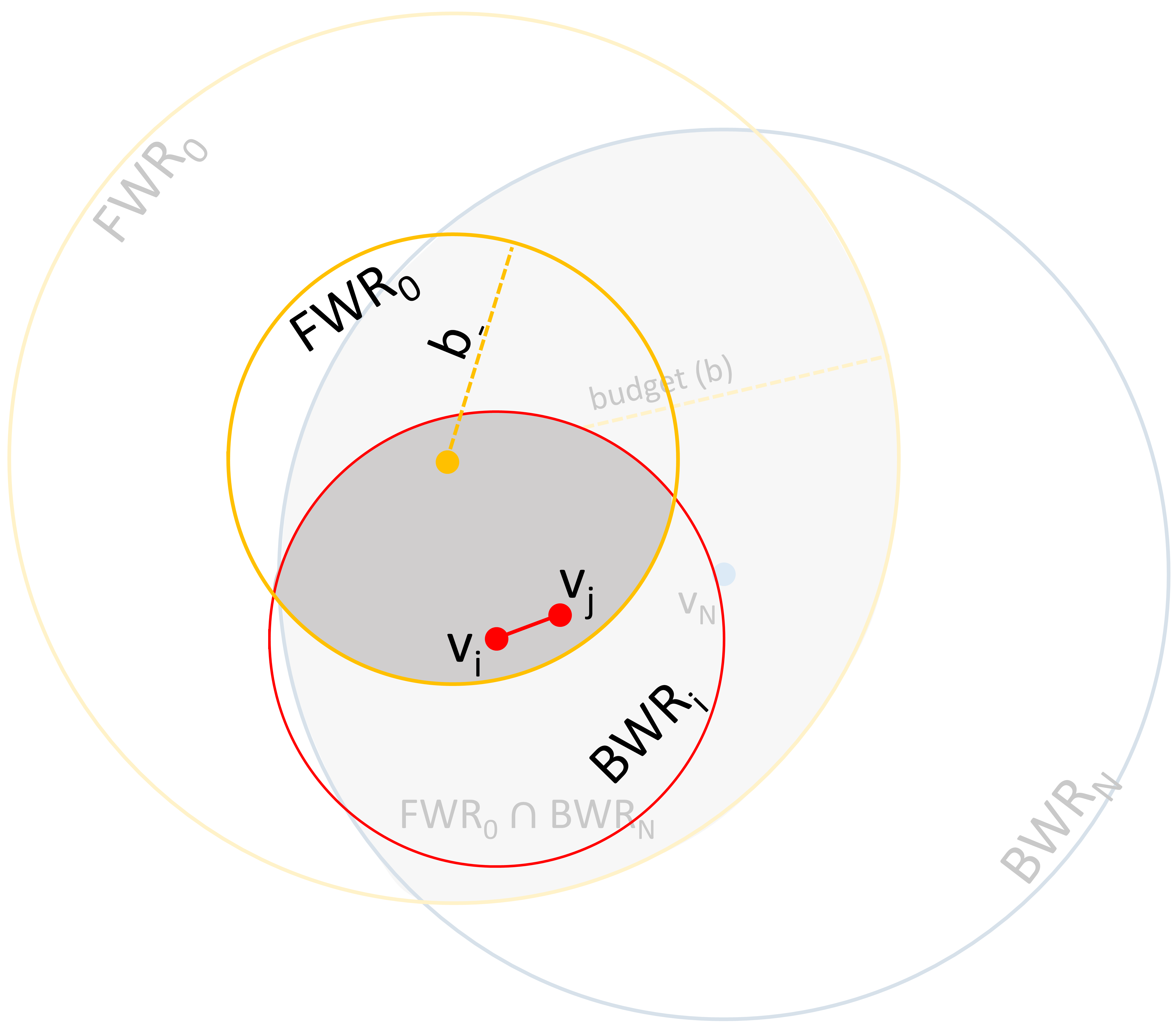
Intuitively, all forward-reachable vertices lie in a quasi-circular region around the source. This region is similar to the circular expansion of a Dijkstra-search. The difference is that in this case the cost criterion is time-dependent travel time. Analogously, all backward-reachable vertices lie in a quasi-circular region around the destination. This graphical intuition is visualized in Figure 2(a). If the destination is not forward-reachable from the source (and/or vice versa), then the query has no answer.
Our solution to the 2TD-AOP is based on an extension of this observation: For an arc to be part of a feasible path, it is a necessary condition that is forward-reachable from the source and is backward-reachable from the destination . Hence, if an arc is not contained in the intersection of the forward-reachability region and the backward-reachability region, it cannot be part of a feasible path. This property will be proved later on. In our solution to the 2TD-AOP, arcs which increase the value are recursively inserted until the budget is exhausted. With every insertion of an arc, the overall travel time of the path increases. Hence, the reachability regions iteratively contract until no more arcs can be inserted. Before we detail this approach in the next section, let us explain the above definitions and their computation with an example.


The definitions are visualized in Figure 3. Figure 3(a) shows a graph with source and destination . Departure time is , and let the time budget . The time-dependent travel times along the arcs are visualized in Figure 3(b). The arcs in Figure 3(a) are labeled with letters which correspond to the travel time functions in Figure 3(b). Figure 3(c) shows the earliest arrivals and latest departures according to this query. If not indicated otherwise, vertices are forward-reachable as well as backward-reachable. The earliest arrivals are computed as in the definition. For example, , implying that the fastest path from at arrives at at time .
Consider the following path:
Since there is no shorter path from to , is not FWR within the given budget. From there are two feasible paths to :
Which of the two constitutes the optimal path depends on the time-dependent value functions and will be discussed later on.
Let us turn to the computation of the latest departures. For example, , implying that in order to arrive at no later than , one must depart at time . Now, consider : the only path to the destination follows the arc . Departing at time results in exceeding the budget, since . The same holds for time . However, when departing at , then , resulting in an arrival within the budget . Hence, in order to compute the latest departure time of a vertex a linear scan among the time windows might be required. Note that the difference between “at time ” and “before time ” is infinitesimal. In theory we set the latest departure at to , in practice, we adjust it by a sufficiently small number. Let us note that this special case only occurs if the latest departure at a vertex by chance coincides with the border between two time windows which is very unlikely in practice. Finally, we prove that in order to compute all feasible paths it suffices to consider the vertices which are forward-reachable and backward-reachable.
Lemma 1
All vertices along all feasible paths are contained in the intersection of the sets of forward-reachable and backward-reachable vertices.
Proof 4.1.
Suppose there exists a feasible path visiting a vertex . Case 1: , this implies , meaning that the subpath from to already exceeds the budget, which contradicts the assumption that is feasible. Case 2: Analogously, if , then , hence cannot be a feasible path.
5 Computing Reachability
Having clarified the importance of the sets of reachable vertices, we will now go into detail on their computation. Both sets are generated by expansions around source and destination with “time-radius ”. By the above lemma, all vertices along all feasible paths are contained in the intersection of the two reachability regions.
In order to compute the set of forward-reachable vertices (for a given source , departure time , and a time budget ), we perform a modified time-dependent all-target Dijkstra search starting at at time , called FWR and illustrated in Algorithm 1. All earliest arrival times are initialized as except for the source for which it is . Additional to a result set containing all visited vertices, we maintain a priority queue containing vertices sorted in ascending order by the earliest arrival time of each vertex. In every iteration, the top element of the queue is removed. In the for-loop spanning lines 8-21, the outgoing arcs of the current vertex are explored. In line 9, the travel time from to its neighbor is added to the earliest arrival time at . If this value does not exceed the budget , is forward-reachable. If was previously not visited, is set accordingly and is added to the queue as well as the result set. If was previously visited and the updated earliest arrival time is better than the previous, it is updated accordingly. Note that once a vertex has been dequeued, the label is final. This is equivalent to the Dijkstra property which ensures that any processed vertex is reached by the shortest path, in this case the fastest time-dependent path. Finally, the result set contains all vertices reachable from the source within the budget.
The set of backward-reachable vertices is computed in a similar fashion but slightly more complicated. The procedure is presented in Algorithm 2 and called BWR. In addition to the result set containing all backward-reachable vertices, we maintain a queue of vertices sorted in descending order by . Initially, the latest departure at the destination is set to the latest possible arrival time, . The algorithm operates backwards from the destination, following incoming arcs which are explored in the for-loop spanning lines 8-25. As was illustrated in the above example (Figure 3), in order to find the latest departure, it is required to linearly scan the time windows. When exploring an incoming arc from to , is initially set to the latest time window not exceeding the latest departure from . If at the travel time from to is too high (i.e., cannot be reached in time for its latest departure), is decremented implying an earlier departure at but possibly also a different travel time along the arc. Note the in line 13, corresponding to the aforementioned special case that for some . In this case, is decreased by a small number in order to avoid computational errors which may occur at time window boundaries. Once a valid latest departure time for is found, is set accordingly. If was previously visited, is only set if it is later than the previous latest departure. Upon termination, all vertices which are backward-reachable from the destination within the given budget are in the result set and labeled with their respective latest departure.
6 Computing Solutions
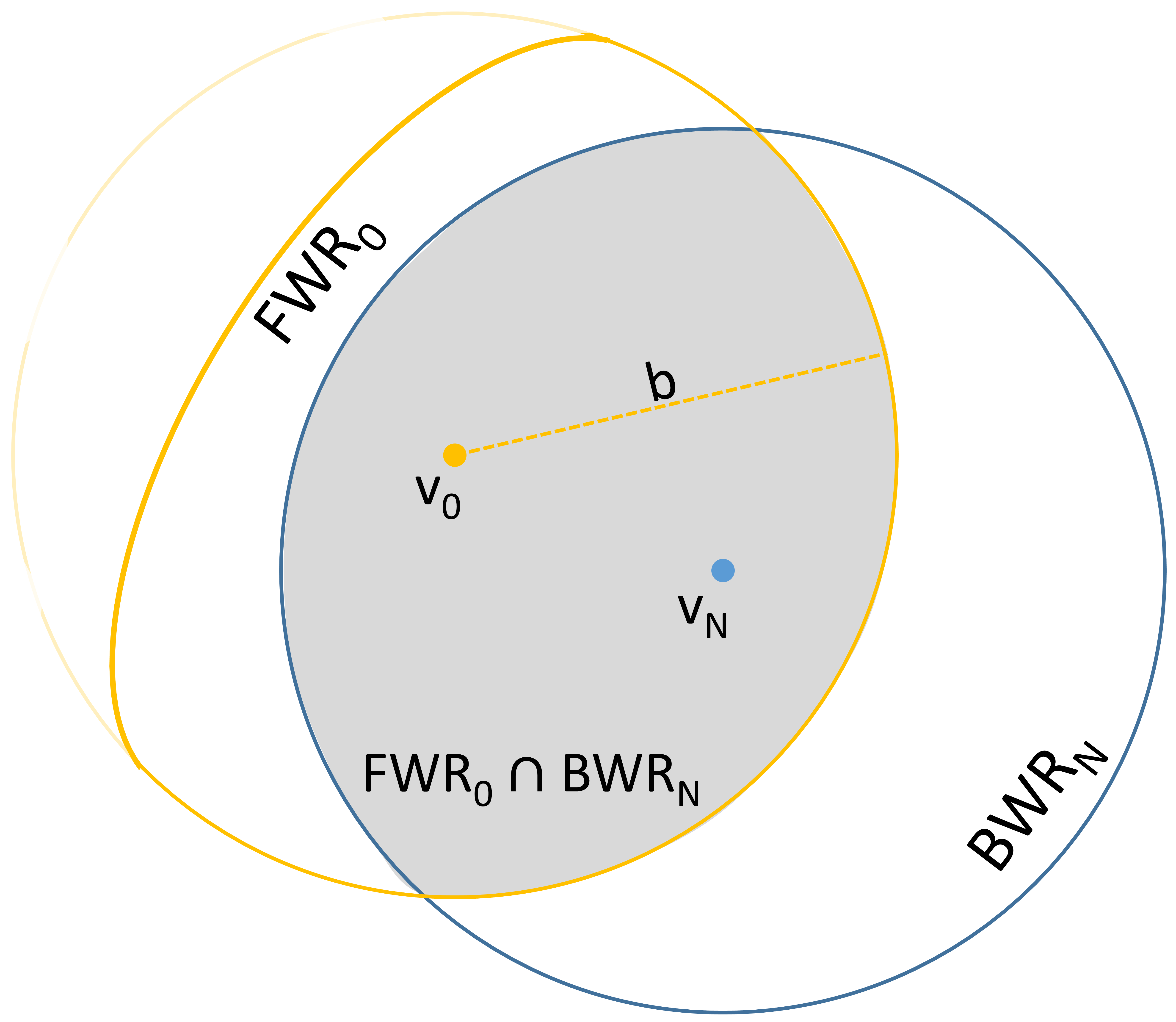
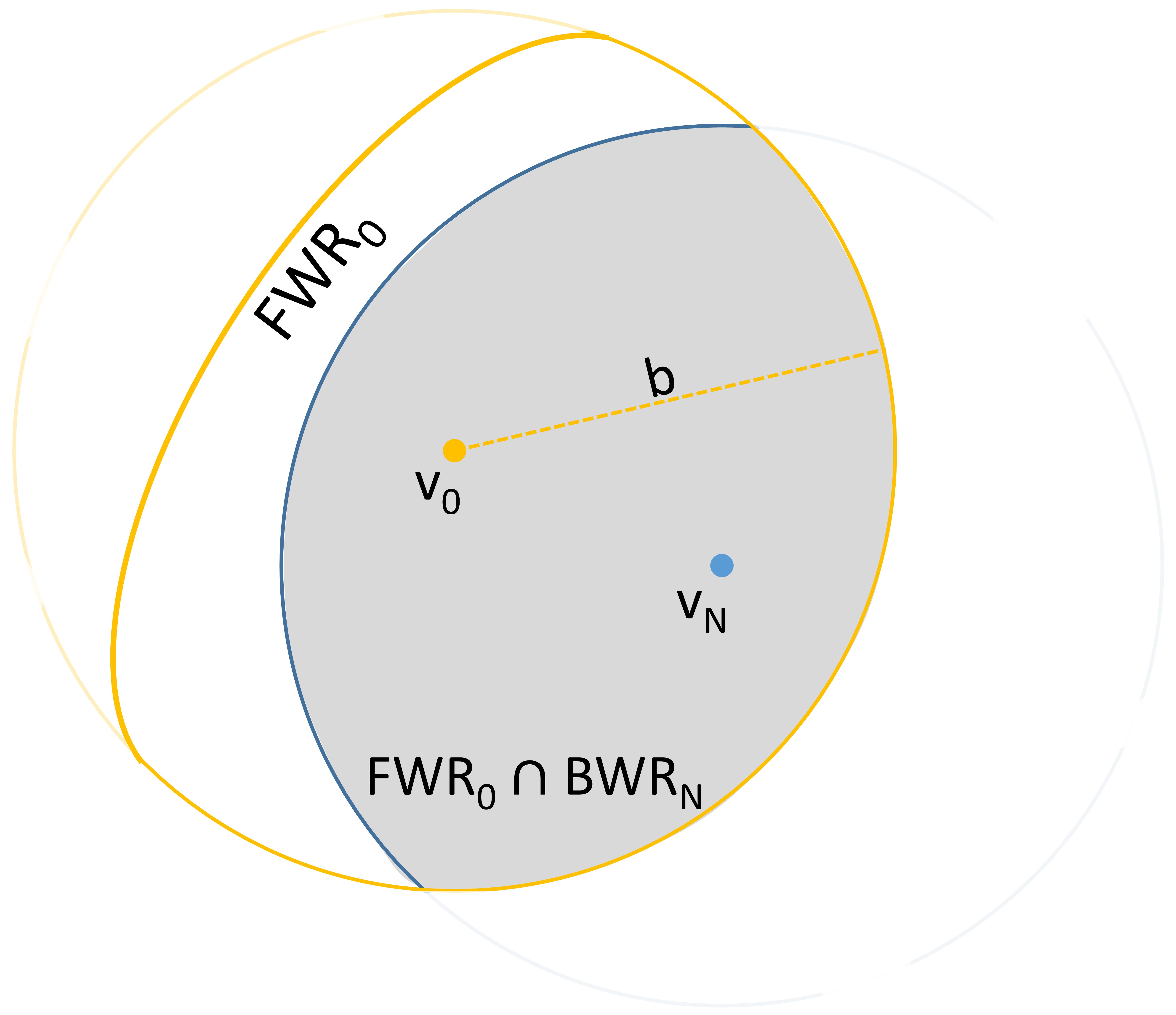
Due to the NP-hardness of the problem, we forgo giving an optimal solution as it would not meet our requirements of providing solutions on large graphs in efficient time. Instead, we propose a heuristic solution to the
Problem 1.
. So far no other solution to the