Optimal Placement and Sizing of Distributed Battery Storage in Low Voltage Grids using Receding Horizon Control Strategies

Abstract

In this paper we present a novel methodology for leveraging Receding Horizon Control (RHC), also known as Model Predictive Control (MPC) strategies for distributed battery storage in a planning problem using a Benders decomposition technique. Longer prediction horizons lead to better storage placement strategies but also higher computational complexity that can quickly become computationally prohibitive. The MPC strategy proposed here in conjunction with a Benders decomposition technique effectively reduces the computational complexity to a manageable level. We use the CIGRE low voltage (LV) benchmark grid as a case study for solving an optimal placement and sizing problem for different control strategies with different MPC prediction horizons. The objective of the MPC strategy is to maximize the photovoltaic (PV) utilization and minimize battery degradation in a local residential area, while satisfying all grid constraints. For this case study we show that the economic value of battery storage is higher when using MPC based storage control strategies than when using heuristic storage control strategies, because MPC strategies explicitly exploit the value of forecast information. The economic merit of this approach can be further increased by explicitly incorporating a battery degradation model in the MPC strategy.

Nomenclature

$\alpha$

proxy subproblem costs

$\alpha_{\mathrm{down}}$

lower bound of proxy subproblem costs

$\boldsymbol{\lambda}^{[j]}$

subproblem dual vector

$\boldsymbol{\lambda}_{\mathrm{s}}$

weighted dual vector

$\eta_{\mathrm{dis},i},\eta_{\mathrm{ch},i}$

battery discharging and charging efficiency

$\boldsymbol{a}_{1},\boldsymbol{a}_{2},\boldsymbol{a}_{3}$

degradation plane parameter vectors

$\boldsymbol{A}^{[j]}$

partitioned subproblem inequality matrix

[][t]l $\boldsymbol{A}$_deg^u, $\boldsymbol{A}$_deg^D,
$\boldsymbol{A}$_deg^u, $\boldsymbol{A}$_deg^z

matrices to include battery degradation for multiple battery systems and time steps

$\boldsymbol{A}_{\mathrm{cost}}^{x},\boldsymbol{A}_{\mathrm{cost}}^{y}$

generator cost matrices for single shot problem

$\tilde{\boldsymbol{A}}_{\mathrm{cost}}^{x},\tilde{\boldsymbol{A}}_{\mathrm{cost}}^{y}$

generator cost matrices for the multiperiod OPF problem

$\boldsymbol{A}_{\mathrm{g}}^{\mathrm{eq}},\boldsymbol{A}_{\mathrm{g}}^{\mathrm{in}}$

grid matrices for single shot problem

$\tilde{\boldsymbol{A}}_{\mathrm{g}}^{\mathrm{eq}},\tilde{\boldsymbol{A}}_{\mathrm{g}}^{\mathrm{in}}$

grid matrices for the multiperiod OPF problem

$\boldsymbol{A}_{q}$

matrix to describe polygonal P,Q regions

$\boldsymbol{A}_{\mathrm{s}}$

intertemporal storage coupling matrix

$\boldsymbol{b}^{\mathrm{c}}_{i}$

offset vector for generator cost segments

$\boldsymbol{b}^{[j]}$

partitioned subproblem right hand vector

$\boldsymbol{b}_{\mathrm{deg}}$

column vector to include battery degradation

$\boldsymbol{b}_{\mathrm{cost}}$

cost offset vector for the single shot problem

$\tilde{\boldsymbol{b}}_{\mathrm{cost}}$

cost offset vector for the multiperiod problem

$\boldsymbol{b}_{\mathrm{g}}^{\mathrm{eq}},\boldsymbol{b}_{\mathrm{g}}^{\mathrm{in}}$

grid related column vectors for the single shot problem

$\tilde{\boldsymbol{b}}_{\mathrm{g}}^{\mathrm{eq}},\tilde{\boldsymbol{b}}_{\mathrm{g}}^{\mathrm{in}}$

grid related column vectors for the multi-period problem

$\boldsymbol{b}$

loss plane offset vector

$\boldsymbol{b}_{\mathrm{s}}$

storage coupling right hand vector

$\boldsymbol{B}$

battery system control input matrix

$\boldsymbol{B}_{\mathrm{r}}$

branch flow matrix

$\boldsymbol{B}_{\mathrm{v}}$

linearized active and reactive power to voltage matrix

$\boldsymbol{B}_{q}$

matrix to describe polygonal P,Q regions

$c$

update cycle

$c_{i}^{\mathrm{net}}$

net power costs and feed-in tariff in €/MWh

$c_{1}^{\mathrm{pv}}$

PV generator costs in €/MWh

$c_{1}^{\mathrm{s}}$

battery generator costs in €/MWh

$\boldsymbol{c}_{i}$

gradient vector for generator cost segments

$\boldsymbol{c}_{\mathrm{s}}$

equivalent battery cost vector in €/kWh

$\boldsymbol{c}_{\mathrm{d}}$

battery cost vector in €/kWh

$\boldsymbol{C}_{\mathrm{g}}$

controllable generator to bus mapping matrix

$\boldsymbol{C}_{\mathrm{pv}}$

PV generator to decisioin variable matrix

$\boldsymbol{C}_{\mathrm{s}}$

battery to decision variable mapping matrix

$\boldsymbol{d}_{k}\in\boldsymbol{D}$

decision vector for battery degradation

$E_{\mathrm{ld}}$

yearly energy consumption

$E_{\mathrm{net}}^{\mathrm{im}}$

yearly imported energy from the feeder

$\boldsymbol{e}$

state of energy vector

$\boldsymbol{e}(0)$

initial state of energy vector

$\boldsymbol{E}$

state of energy evolution vector

$H$

control horizon

$\boldsymbol{i}_{\mathrm{b}}$

branch current vector in p.u.

$\boldsymbol{i}_{\mathrm{b}}^{\mathrm{max}}$

max branch current vector in p.u.

$\boldsymbol{i}^{0},\boldsymbol{i}^{1}$

supporting current vectors for piecewise linear loss approximation

$j$

subproblem index

$J_{\mathrm{sub}}$

sum of subproblem objective values

$J_{\mathrm{sub}}^{\mathrm{wS}}$

yearly revenue with battery storage

$J_{\mathrm{sub}}^{\mathrm{w/oS}}$

yearly revenue without battery storage

$J^{[j]}$

subproblem objective value

$k$

time step

$l$

Benders stage

$\boldsymbol{L}_{0},\boldsymbol{L}_{1}$

supporting plane matrices for piecewise linear loss approximation

$m$

battery lifetime in years

$\boldsymbol{M}_{\mathrm{f}}$

bus-injection to branch-current matrix

$\boldsymbol{M}$

reduced bus-injection to branch-current matrix

$n$

number of subproblems

$n_{\mathrm{b}}$

number of buses

$n_{\mathrm{c}}$

number of linear constraints

$n_{\mathrm{d}}$

number of decision variables

$n_{\mathrm{g}}$

number of controllable generators

$n_{\mathrm{l}}$

number of branches

$n_{\mathrm{pv}}$

number of PV units

$n_{\mathrm{p}}$

number of planes

$n_{s}$

number of battery systems

$N$

investment horizon

$p_{\mathrm{bat}}$

active battery stack power

$\boldsymbol{p}$

nodal active bus power vector

$\boldsymbol{p}_{\mathrm{d}},\boldsymbol{q}_{\mathrm{d}}$

nodal active and reactive power load vectors

$\boldsymbol{p}_{\mathrm{gen}},\boldsymbol{q}_{\mathrm{gen}}$

active and reactive generator power vectors

[][t]l$\boldsymbol{p}$_gen^pv,$\boldsymbol{q}$_gen^pv,
$\boldsymbol{p}$_gen^pv,^$\boldsymbol{p}$_gen^pv

active and reactive PV generator power and prediction vectors

$\boldsymbol{p}_{\mathrm{gen}}^{\mathrm{s,dis}}$

active discharging battery grid power vector

$\boldsymbol{p}_{\mathrm{gen}}^{\mathrm{s,ch}}$

active charging battery grid power vector

$\boldsymbol{p}_{\mathrm{l}}^{\mathrm{p}},\boldsymbol{p}_{\mathrm{l}}^{\mathrm{q}}$

decision vectors of real network losses

$\boldsymbol{p}_{\mathrm{d}},\boldsymbol{q}_{\mathrm{d}},\hat{\boldsymbol{p}}_{\mathrm{d}}$

active and reactive power load measurement and prediction vectors

$\boldsymbol{p}_{\mathrm{min}},\boldsymbol{p}_{\mathrm{max}}$

min and max active generator power vectors

$\boldsymbol{q}$

nodal reactive bus power vector

$\boldsymbol{R}_{\mathrm{d}}$

diagonal branch resistance matrix in p.u.

$\boldsymbol{s}_{\mathrm{max}}$

max apparent generator power vector

$\boldsymbol{S}_{x},\boldsymbol{S}_{u}$

matrices to describe the storage evolution

$T$

sample time

$\boldsymbol{v}$

nodal line to neutral RMS voltage vector

$\boldsymbol{v}_{\mathrm{min}},\boldsymbol{v}_{\mathrm{max}}$

min and max nodal RMS voltage vectors

$\boldsymbol{v}_{\mathrm{s}}$

slack bus voltage vector

$\boldsymbol{V}_{\mathrm{df}}$

inverse diagonal voltage matrix

$\boldsymbol{x}_{k}\in\boldsymbol{X}$

decision vector for grid variables

$\boldsymbol{X}_{\mathrm{d}}$

diagonal branch reactance matrix in p.u.

$\boldsymbol{y}_{k}\in\boldsymbol{Y}$

generator cost decision vector

$\boldsymbol{z}$

decision vector for battery capacity variables

$\boldsymbol{z}_{\mathrm{max}}$

upper bound for battery capacity variables

$Z_{\mathrm{down}}$

lower bound for total profit

$Z_{\mathrm{up}}$

upper bound for total profit

I Introduction

I-A Motivation

Energy storage technologies can have a key role for decarbonizing the power sector [1]. In particular, Distributed Battery Storage (DBS) in Low Voltage (LV) grids is considered to be a promising technology for balancing short-term fluctations and for alleviating grid congestion caused by a high share of distributed photovaltaic (PV) units [2, 3]. Since a large number of PV units is installed in LV grids and since LV grid capacity is typically limited, it can be expected that Distribution System Operators will have to increasingly curtail PV output to mitigate grid congestion. This is already the case in Germany, where more than half of the installed PV power, i.e. 22 GW of 39 GW (2015), is installed in LV grids [4, p. 6] and where PV curtailment has risen more than tenfold in recent years (2012–2015) [4, p. 12]. With more and more roof-top PV units being currently installed in the US, this issue is likely to attract more attention there as well. In this context, DBS configurations can help DSOs to reduce PV curtailment in LV grids. But DBS installations in combination with PV are also able to increase the self-consumption of PV, thereby lowering electricity costs for end-consumers. This is particularly attractive in net-metering tariff schemes. The authors in [5] report that the optimal size and location of storage depend highly on congested lines in transmission networks and hence on the grid topology. This also holds for DBS applications in LV grids, where an optimal DBS scheme can give support for specific lines that would be overloaded under high PV penetration levels.

Furthermore, previous research has drawn attention to Model Predictive Control (MPC) strategies that allow for an optimal predictive dispatch of energy storage in LV grids, for instance [6, 7], in combination with other generation sources. Such strategies solve a multi-period Optimal Power Flow (OPF) problem to optimally schedule generator setpoints over a receding control horizon taking storage dynamics and grid constraints into account. Please note that the application of MPC to power system (dispatch) problems is a long-standing concept, see for example [8, 9]. Varying the prediction horizon of the predictive dispatch optimization has a great influence on how much energy can be shifted within this time window. This implies that the optimal energy storage size heavily depends on the employed operational policy (for an illustrative example cf. [10, p. 203–205]). Hence, there is a clear need to combine grid planning considerations with grid operational aspects.

The main objective of this paper is to develop a planning strategy that leverages MPC control strategies acting on different control horizons to find the optimal location and size of DBS in LV grids.

I-B Related Work

Recent studies [11, 1, 12, 13] evaluate the economic value of energy storage without considering the grid topology. In contrast, the papers [14, 15, 5, 16, 17, 18] incorporate a grid model. They solve a multi-period OPF problem over a fixed finite control horizon e.g. 24 hours to obtain the optimal location and size of the storage devices and do not consider the influence of seasonality. By solving a finite horizon problem, the optimal siting results would be different for different seasons, i.e. in summer due to high PV irradiation storage capacities would be bigger than in winter. According to [14] enlarging the horizon makes the siting problem computationally intractable. For this reason, [14] proposes a heuristic to find the best storage locations and capacities by comparing a sequence of multi-period problems resulting in a near-optimal allocation of DBS or [16] solves a finite problem over four representative days from each season following that the variability within each season cannot be captured. Moreover, considering long horizons does not reflect the operational strategy, since in reality predictive dispatch methods can only act on shorter horizons e.g. in the presence of predictive Receding Horizon Control (RHC) strategies. This is due to the fact that accurate weather and load predictions are only available for limited periods in advance.

The methods from [12, 13, 14, 15, 5] can deal with uncertainty of PV infeed and load consumption by either solving consecutively-cycled multi-period problems over the course of a reference year [14, 15], a stochastic dynamic programming problem [12, 13], or for a defined set of PV and load scenarios [5].

To further reduce the computational complexity, [14, 15, 5] include the so-called DC power flow approximation. Unfortunately, a DC power flow approximation is not applicable for LV grids, since active power flow is determined by voltage magnitude differences and not by voltage angle differences as it would be the case in transmission grids. The authors in [17, 18] incorporate a semi-definite power flow relaxation, which is still hard to solve. The authors of [19] incorporate the operational strategy inside a sub-optimal greedy heuristic algorithm that determines the optimal storage size and location. Another way to tackle such complex problems is to decompose the problem into subproblems. This is done in [20, 21] by either using Benders decomposition [20] or via an alternate direction method of multipliers [21]. In addition, none of the papers include a battery degradation objective in the operational strategy to take battery lifetime into account.

I-C Contribution

The main contribution of this paper is two-fold. First, we develop a Benders decomposition algorithm for DBS applications that links the operational domain with the planning domain. Our approach decomposes with respect to time the sizing and placement problem into a tractable master problem and subproblems. This allows us to account for PV and load uncertainty in the same way as proposed in [14] by incorporating different PV and load realizations inside the coupled subproblems that can be considered as different scenarios. Second, to demonstrate the usefulness of our approach, we present a cost analysis that assesses at which storage cost levels and under which operational strategy a DBS investment becomes viable. In our previous work [22] we developed a linearized OPF scheme for LV grids and incorporated the resulting Linear Programming (LP) problem in a multi-period OPF problem to solve an optimal placement and sizing problem for an infinite control horizon. As an extension we incorporate our linearized OPF scheme into an MPC control strategy that reflects the operational strategy. The objective of the MPC strategy is to maximize the PV utilization, while taking battery degradation into account and complying with grid constraints in a local residential area. Unlike [23] the subproblems cannot be solved in a parallel fashion, since storage induces an inherent intertemporal coupling between the subproblems. Nevertheless, we show how we can formulate a Benders decomposition algorithm for this problem class, which significantly reduces the computational effort.

The remainder of this paper is organized as follows. Section II defines the problem that we aim to solve. Section III reviews the optimal placement and sizing problem and describes the proposed Benders decomposition method. Section IV presents the simulation results and an economic assessment. Finally, Section V presents the conclusions.

II Problem Definition

Figure 1: Illustration of the local control area. The overall objective of the proposed MPC strategy is to maximize PV utilization and to minimize battery degradation. Dual variables and decision variables are exchanged between planning master problem and MPC storage control strategy.

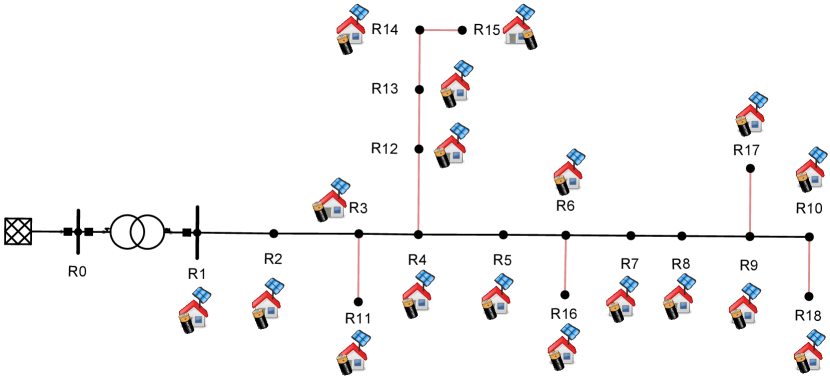
This section defines the problem that we aim to solve. Figure 1 illustrates the test case environment. We assume that we have a residential local control area with a group of so-called prosumers that have installed PV generators and battery systems. The energy capacities $\boldsymbol{z}$ are determined by the planning master problem. The area has a centralized local area control entity and a communication infrastructure. The storage control entity is an MPC controller that incorporates a multi-period distribution-level OPF and acts as a scheduler with control horizons ranging from 24 hours to 1 month. By using an OPF method, we enable the optimal utilization of the grid and make use of optimal Active Power Curtailment (APC) and Reactive Power Control (RPC). We solve a multi-period problem considering a two-tariff price scenario and a feed-in tariff for the net power $p_{\mathrm{gen}}^{\mathrm{net}}$. In this way, we impose that the scheduler exploits the price differences from the tariff scheme and maximizes the self-consumption of PV in the local area. In addition, we incorporate a battery degradation objective to assess when revenue benefits outweigh degradation cost. The MPC controller gets perfect load $\hat{\boldsymbol{p}}_{\mathrm{d}}$ and solar $\hat{\boldsymbol{p}}_{\mathrm{gen}}^{\mathrm{pv}}$ forecast time-series and schedules the control inputs of the real and reactive powers for the batteries $p_{\mathrm{gen}}^{\mathrm{s}},q_{\mathrm{gen}}^{\mathrm{s}}$ and the PV generators $p_{\mathrm{gen}}^{\mathrm{pv}},q_{\mathrm{gen}}^{\mathrm{pv}}$. It has also the knowledge of the State of Energy (SoE) of the batteries acting as a feedback signal to run a new optimization cycle. To account for energy, the SoE definition is needed. It differs from the State of Charge (SoC) due to the nonlinear relationship between open-circuit potential and charge. The dual variables $\boldsymbol{\lambda}_{\mathrm{s}}$ need to be exchanged with the planning problem to initiate a new iteration of the Benders decomposition.

III Optimal Placement and Sizing Problem

III-A Linearized OPF Problem

In our previous work [22] we developed a linearized OPF method for radial LV networks. Here, we extend our method to incorporate any convex generator cost function and summarize the linear approximations for voltage, branch flow, and network power losses from [22].

III-A1 Voltage Approximation

Under the assumption of a high $R/X$ ratio, the absolute voltage magnitude drops along $n_{\mathrm{l}}$ lines in a radial balanced grid are linearly approximated by

$$\boldsymbol{v}-\boldsymbol{v}_{\mathrm{s}}\approx\underbrace{\left[\boldsymbol{M}^{T}\boldsymbol{R}_{\mathrm{d}}\boldsymbol{M}_{\mathrm{f}}{\boldsymbol{V}}_{\mathrm{df}}\quad\boldsymbol{M}^{T}\boldsymbol{X}_{\mathrm{d}}\boldsymbol{M}_{\mathrm{f}}{\boldsymbol{V}}_{\mathrm{df}}\right]}_{\boldsymbol{B}_{\mathrm{v}}}\left[\begin{array}[]{c}\boldsymbol{p}\\ \boldsymbol{q}\end{array}\right],$$ (1)

where $\boldsymbol{v}\in\mathbb{R}^{n_{\mathrm{l}}\times 1}$ is the nodal absolute voltage magnitude vector in per unit and $\boldsymbol{v}_{\mathrm{s}}\in\mathbb{R}^{n_{\mathrm{l}}\times 1}$ is the absolute voltage magnitude vector for the slack bus in per unit. The vectors $\boldsymbol{p},\boldsymbol{q}\in\mathbb{R}^{n_{\mathrm{b}}\times 1}$ are the nodal per unit injections for active and reactive power for $n_{\mathrm{b}}$ buses. The matrix $\boldsymbol{M}_{\mathrm{f}}\in\mathbb{R}^{n_{\mathrm{l}}\times n_{\mathrm{b}}}$ maps the bus-injection currents to branch-currents and is also called the bus-injection to branch-current (BIBC) matrix. Here, we also define a reduced version of $\boldsymbol{M}_{\mathrm{f}}$ indicated with $\boldsymbol{M}\in\mathbb{R}^{n_{\mathrm{l}}\times n_{\mathrm{b}}-1}$, in which the row of the involved slack bus is deleted. $\boldsymbol{R}_{\mathrm{d}}^{n_{\mathrm{l}}\times n_{\mathrm{l}}}=\mathrm{diag}\{r_{\mathrm{d}1},...,r_{\mathrm{d}n_{\mathrm{l}}}\}$ is the branch resistance matrix in per unit and $\boldsymbol{X}_{\mathrm{d}}^{n_{\mathrm{l}}\times n_{\mathrm{l}}}=\mathrm{diag}\{x_{\mathrm{d}1},...,x_{\mathrm{d}n_{\mathrm{l}}}\}$ is the reactance matrix in per unit. The matrix ${\boldsymbol{V}}_{\mathrm{df}}\in\mathbb{R}^{n_{\mathrm{b}}\times n_{\mathrm{b}}}$ includes the inverse nodal complex voltages of the grid and is defined as

$${\boldsymbol{V}}_{\mathrm{df}}=|\mathrm{diag}\{1/\underline{v}_{1},\ldots,1/\underline{v}_{n_{\mathrm{b}}}\}^{*}|\quad.$$ (2)

III-A2 Branch Flow Approximation

If we assume that the reactive power injections are much smaller than the active power injections, which holds for normal grid operation in LV grids, we can neglect the contribution on the reactive power by approximating

$$\boldsymbol{i}_{\mathrm{b}}\approx\underbrace{\boldsymbol{M}_{\mathrm{f}}{\boldsymbol{V}}_{\mathrm{df}}}_{\boldsymbol{B}_{\mathrm{r}}}\boldsymbol{p}\quad,$$ (3)

where $\boldsymbol{i}_{\mathrm{b}}\in\mathbb{R}^{n_{\mathrm{l}}\times 1}$ is the current branch flow magnitude vector in per unit.

III-A3 Loss Approximation

We approximate active network power losses by

$$\boldsymbol{p}_{\mathrm{l}}^{\mathrm{p}} \approx\max\left\{\boldsymbol{L}_{0}\boldsymbol{p},-\boldsymbol{L}_{0}\boldsymbol{p},\boldsymbol{L}_{1}\boldsymbol{p}+\boldsymbol{b},-\boldsymbol{L}_{1}\boldsymbol{p}+\boldsymbol{b}\right\}\quad,$$ (4)

$$\boldsymbol{p}_{\mathrm{l}}^{\mathrm{q}} \approx\max\left\{\boldsymbol{L}_{0}\boldsymbol{q},-\boldsymbol{L}_{0}\boldsymbol{q},\boldsymbol{L}_{1}\boldsymbol{q}+\boldsymbol{b},-\boldsymbol{L}_{1}\boldsymbol{q}+\boldsymbol{b}\right\}\quad.$$ (5)

where

$$\boldsymbol{L}_{0} = \mathrm{diag}\{i^{0}_{1},\cdots,i^{0}_{n_{\mathrm{l}}}\}\boldsymbol{R}_{\mathrm{d}}\boldsymbol{M}_{\mathrm{f}}{\boldsymbol{V}}_{\mathrm{df}}\quad,$$ (6)

$$\boldsymbol{L}_{1} = \mathrm{diag}\{i^{0}_{1}+i^{1}_{1},\cdots,i^{0}_{n_{\mathrm{l}}}+i^{1}_{n_{\mathrm{l}}}\}\boldsymbol{R}_{\mathrm{d}}\boldsymbol{M}_{\mathrm{f}}{\boldsymbol{V}}_{\mathrm{df}}\quad,$$ (7)

$$\boldsymbol{b} = -[r_{1}i^{0}_{1}i^{1}_{1},\cdots,r_{n_{\mathrm{l}}}i^{0}_{n_{\mathrm{l}}}i^{1}_{n_{\mathrm{l}}}]^{T}\quad.$$ (8)

The power line loss vectors $\boldsymbol{p}_{\mathrm{l}}^{\mathrm{p}}\in\mathbb{R}^{n_{\mathrm{l}}\times 1}$ and $\boldsymbol{p}_{\mathrm{l}}^{\mathrm{q}}\in\mathbb{R}^{n_{\mathrm{l}}\times 1}$ are the real network power losses resulting from active and reactive power injections. Equations (6)-(8) define hyperplanes with the supporting currents $\boldsymbol{i}_{0},\boldsymbol{i}_{1}$ for the power losses that are inner approximations of the quadratic power loss functions.

III-A4 Forward Backward Sweep Optimal Power Flow (FBS-OPF) Formulation

With the presented approximations we can state a linearized OPF problem. Since the approximations are in the Forward Backward Sweep (FBS) load flow framework [24], we call our linearized method FBS-OPF. We first define the optimization vector $\boldsymbol{x}=\left[\boldsymbol{p}_{\mathrm{l}}^{\mathrm{p}},\boldsymbol{p}_{\mathrm{l}}^{\mathrm{q}},\boldsymbol{p}_{\mathrm{gen}},\boldsymbol{q}_{\mathrm{gen}},\boldsymbol{v}\right]^{T}$ reflecting all grid related variables. The helper decision vector $\boldsymbol{y}\in\mathbb{R}^{n_{\mathrm{g}}\times 1}$ specifies the generation costs for $n_{\mathrm{g}}$ generators. The objective is to find the optimal generator setpoints $\boldsymbol{p}_{\mathrm{gen}},\boldsymbol{q}_{\mathrm{gen}}$ that minimize the generation costs, while satisfying all grid constraints. The active and reactive generator bus injections $\boldsymbol{p}_{\mathrm{gen}}\in\mathbb{R}^{n_{\mathrm{g}}\times 1}$ and $\boldsymbol{q}_{\mathrm{gen}}\in\mathbb{R}^{n_{\mathrm{g}}\times 1}$ are mapped to the buses with the matrix $\boldsymbol{C}_{\mathrm{g}}\in\mathbb{R}^{n_{\mathrm{b}}\times n_{\mathrm{g}}}$.

The extended linearized optimization problem is then:

$$\begin{array}[]{lllll}\lx@intercol J^{*}=\displaystyle\min_{\boldsymbol{x},\boldsymbol{y}}\boldsymbol{1}^{T}\boldsymbol{y}\hfil\lx@intercol\\ &\text{s.t.}\\ &\text{(a)}&\left[\begin{array}[]{@{\hspace{2pt}}c@{\hspace{2pt}}c@{\hspace{2pt}}c@{\hspace{2pt}}}\hskip 2.0pt\lx@intercol\hfil\boldsymbol{c}_{1}\hfil\hskip 2.0&\hfil\hskip 2.0&\hfil\hskip 2.0\\ \hskip 2.0pt\lx@intercol\hfil\hfil\hskip 2.0&\ddots\hfil\hskip 2.0&\hfil\hskip 2.0\\ \hskip 2.0pt\lx@intercol\hfil\hfil\hskip 2.0&\hfil\hskip 2.0&\boldsymbol{c}_{n_{\mathrm{g}}}\hfil\hskip 2.0\end{array}\right]\boldsymbol{p}_{\mathrm{gen}}-\left[\begin{array}[]{@{\hspace{2pt}}c@{\hspace{2pt}}c@{\hspace{2pt}}c@{\hspace{2pt}}}\hskip 2.0pt\lx@intercol\hfil\boldsymbol{1}\hfil\hskip 2.0&\hfil\hskip 2.0&\hfil\hskip 2.0\\ \hskip 2.0pt\lx@intercol\hfil\hfil\hskip 2.0&\ddots\hfil\hskip 2.0&\hfil\hskip 2.0\\ \hskip 2.0pt\lx@intercol\hfil\hfil\hskip 2.0&\hfil\hskip 2.0&\boldsymbol{1}\hfil\hskip 2.0\end{array}\right]\boldsymbol{y}\leq-\left[\begin{array}[]{c}\boldsymbol{b}^{\mathrm{c}}_{1}\\ \vdots\\ \boldsymbol{b}^{\mathrm{c}}_{n_{\mathrm{g}}}\end{array}\right]\\ &\text{(b)}&\lx@intercol\boldsymbol{1}^{T}\boldsymbol{C}_{\mathrm{g}}\boldsymbol{p}_{\mathrm{gen}}-\boldsymbol{1}^{T}\boldsymbol{p}_{\mathrm{l}}^{\mathrm{p}}-\boldsymbol{1}^{T}\boldsymbol{p}_{\mathrm{l}}^{\mathrm{q}}=\boldsymbol{1}^{T}\boldsymbol{p}_{\mathrm{d}}\hfil\lx@intercol\\ &\text{(c)}&\lx@intercol\boldsymbol{B}_{\mathrm{v}}\left[\begin{array}[]{l}\boldsymbol{C}_{\mathrm{g}}\boldsymbol{p}_{\mathrm{gen}}\\ \boldsymbol{C}_{\mathrm{g}}\boldsymbol{q}_{\mathrm{gen}}\end{array}\right]-\boldsymbol{v}=\boldsymbol{B}_{\mathrm{v}}\left[\begin{array}[]{l}\boldsymbol{p}_{\mathrm{d}}\\ \boldsymbol{q}_{\mathrm{d}}\end{array}\right]-\boldsymbol{v}_{\mathrm{s}}\hfil\lx@intercol\\ &\text{(d)}&\lx@intercol\boldsymbol{p}_{\mathrm{l}}^{\mathrm{p}}-\boldsymbol{L}_{0}\boldsymbol{C}_{\mathrm{g}}\boldsymbol{p}_{\mathrm{gen}}\geq-\boldsymbol{L}_{0}\boldsymbol{p}_{\mathrm{d}}\hfil\lx@intercol\\ &\text{(e)}&\lx@intercol\boldsymbol{p}_{\mathrm{l}}^{\mathrm{p}}+\boldsymbol{L}_{0}\boldsymbol{C}_{\mathrm{g}}\boldsymbol{p}_{\mathrm{gen}}\geq\boldsymbol{L}_{0}\boldsymbol{p}_{\mathrm{d}}\hfil\lx@intercol\\ &\text{(f)}&\lx@intercol\boldsymbol{p}_{\mathrm{l}}^{\mathrm{p}}-\boldsymbol{L}_{1}\boldsymbol{C}_{\mathrm{g}}\boldsymbol{p}_{\mathrm{gen}}\geq-\boldsymbol{L}_{1}\boldsymbol{p}_{\mathrm{d}}+\boldsymbol{b}\hfil\lx@intercol\\ &\text{(g)}&\lx@intercol\boldsymbol{p}_{\mathrm{l}}^{\mathrm{p}}+\boldsymbol{L}_{1}\boldsymbol{C}_{\mathrm{g}}\boldsymbol{p}_{\mathrm{gen}}\geq+\boldsymbol{L}_{1}\boldsymbol{p}_{\mathrm{d}}+\boldsymbol{b}\hfil\lx@intercol\\ &\text{(h)}&\lx@intercol\boldsymbol{p}_{\mathrm{l}}^{\mathrm{q}}-\boldsymbol{L}_{0}\boldsymbol{C}_{\mathrm{g}}\boldsymbol{q}_{\mathrm{gen}}\geq-\boldsymbol{L}_{0}\boldsymbol{q}_{\mathrm{d}}\hfil\lx@intercol\\ &\text{(i)}&\lx@intercol\boldsymbol{p}_{\mathrm{l}}^{\mathrm{q}}+\boldsymbol{L}_{0}\boldsymbol{C}_{\mathrm{g}}\boldsymbol{q}_{\mathrm{gen}}\geq\boldsymbol{L}_{0}\boldsymbol{q}_{\mathrm{d}}\hfil\lx@intercol\\ &\text{(j)}&\lx@intercol\boldsymbol{p}_{\mathrm{l}}^{\mathrm{q}}-\boldsymbol{L}_{1}\boldsymbol{C}_{\mathrm{g}}\boldsymbol{q}_{\mathrm{gen}}\geq-\boldsymbol{L}_{1}\boldsymbol{q}_{\mathrm{d}}+\boldsymbol{b}\hfil\lx@intercol\\ &\text{(k)}&\lx@intercol\boldsymbol{p}_{\mathrm{l}}^{\mathrm{q}}+\boldsymbol{L}_{1}\boldsymbol{C}_{\mathrm{g}}\boldsymbol{q}_{\mathrm{gen}}\geq+\boldsymbol{L}_{1}\boldsymbol{q}_{\mathrm{d}}+\boldsymbol{b}\hfil\lx@intercol\\ &\text{(l)}&\lx@intercol-\boldsymbol{i}_{\mathrm{b}}^{\mathrm{max}}+\boldsymbol{B}_{\mathrm{r}}\boldsymbol{p}_{\mathrm{d}}\leq\boldsymbol{B}_{\mathrm{r}}\boldsymbol{C}_{\mathrm{g}}\boldsymbol{p}_{\mathrm{gen}}\leq\boldsymbol{i}_{\mathrm{b}}^{\mathrm{max}}+\boldsymbol{B}_{\mathrm{r}}\boldsymbol{p}_{\mathrm{d}}\hfil\lx@intercol\\ &\text{(m)}&\boldsymbol{v}_{\mathrm{min}}\leq\boldsymbol{v}\leq\boldsymbol{v}_{\mathrm{max}}\\ &\text{(n)}&\boldsymbol{p}_{\mathrm{min}}\leq\boldsymbol{p}_{\mathrm{gen}}\leq\boldsymbol{p}_{\mathrm{max}}\\ &\text{(o)}&-\boldsymbol{s}_{\mathrm{max}}\leq\boldsymbol{p}_{\mathrm{gen}}+\boldsymbol{A}_{q}\boldsymbol{q}_{\mathrm{gen}}\leq\boldsymbol{s}_{\mathrm{max}}\\ &\text{(p)}&-\boldsymbol{s}_{\mathrm{max}}\leq\boldsymbol{p}_{\mathrm{gen}}-\boldsymbol{A}_{q}\boldsymbol{q}_{\mathrm{gen}}\leq\boldsymbol{s}_{\mathrm{max}}\\ &\text{(q)}&-\boldsymbol{B}_{q}\boldsymbol{s}_{\mathrm{max}}\leq\boldsymbol{q}_{\mathrm{gen}}\leq\boldsymbol{B}_{q}\boldsymbol{s}_{\mathrm{max}}\quad,\end{array}$$ (9)

where $\boldsymbol{p}_{\mathrm{d}}\in\mathbb{R}^{n_{\mathrm{b}}\times 1}$ and $\boldsymbol{q}_{\mathrm{d}}\in\mathbb{R}^{n_{\mathrm{b}}\times 1}$ are the active and reactive net load. Constraint (9a) includes the epigraphs of convex piecewise-affine (PWA) generator cost functions, i.e. the set of points lying above the specified cost functions. The vectors $\boldsymbol{c}_{i}\in\mathbb{R}^{n_{\mathrm{ls}}\times 1}$ and $\boldsymbol{b}^{\mathrm{c}}_{i}\in\mathbb{R}^{n_{\mathrm{ls}}\times 1}$ assign the gradients and offsets of the PWA cost function for each generator. The variable $n_{\mathrm{ls}}$ specifies the number of the cost function segments. In this way, we can model the generation costs as a set of linear constraints. Figure 2 illustrates the PWA cost function representation for three line segments and one generator. Constraint (9b) enforces power balance in the grid. The voltage approximation (1) is included in (9c). The constraints (9d-k) incorporate epigraph formulations of (4) and (5) that are piecewise linear inner approximations of the real power losses. Constraint (9l) includes the branch flow limit approximation (3). Constraints (9m,n) specify the lower and upper bounds for the voltage ($\boldsymbol{v}_{\mathrm{min}},\boldsymbol{v}_{\mathrm{max}}$) and active generator powers ($\boldsymbol{p}_{\mathrm{min}},\boldsymbol{p}_{\mathrm{max}}$). Constraints (9o-q) approximate the generators’ apparent power limits, where $\boldsymbol{s}_{\mathrm{max}}$ is the generators’ maximum apparent power; specifically, we define circular-bounded and $\cos\phi$-bounded active and reactive power settings by approximating the circular area/segments with convex sets [25] that describe the polygons depicted in Fig 3.

Figure 2: Piecewise-affine (PWA) cost function representation showing illustratively three line segments to reflect any convex generator cost curves.

Figure 3: Approximated reactive power capability areas a) circular-bounded b) $\cos\phi$-bounded. The polygonal convex regions can be described with the constraints (9h-l). [25]

For the sake of convenience, problem (9) can be written in a more compact form:

$$\begin{array}[]{lll}J^{*}=&\lx@intercol\displaystyle\min_{\boldsymbol{x,y}}\ \boldsymbol{1}^{T}\boldsymbol{y}\hfil\lx@intercol\\ &\text{s.t.}\\ &\text{(a)}&\boldsymbol{A}_{\mathrm{cost}}^{x}\boldsymbol{x}-\boldsymbol{A}_{\mathrm{cost}}^{y}\boldsymbol{y}\leq-\boldsymbol{b}_{\mathrm{cost}}\\ &\text{(b)}&\boldsymbol{A}_{\mathrm{g}}^{\mathrm{in}}\boldsymbol{x}\geq\boldsymbol{b}_{\mathrm{g}}^{\mathrm{in}}\\ &\text{(c)}&\boldsymbol{A}_{\mathrm{g}}^{\mathrm{eq}}\boldsymbol{x}=\boldsymbol{b}_{\mathrm{g}}^{\mathrm{eq}}\\ &\text{(d)}&\boldsymbol{x}_{\mathrm{min}}\leq\boldsymbol{x}\leq\boldsymbol{x}_{\mathrm{max}}\quad,\end{array}$$ (10)

where constraint (10a) incorporates (9a), (10b) incorporates (9d-l,o-q), (10c) incorporates (9b,c), and (10d) incorporates (9m,n).

III-B Multi-period Problem

Since energy storage introduces an intertemporal coupling into our dispatch problems, the placement and sizing problem has to be formulated as a multi-period problem over a given investment horizon $N$. By incorporating the single shot solutions of (10), the purpose is to find the optimal placement and sizes of storage devices, while considering a certain operational strategy. We introduce a further optimization vector $\boldsymbol{z}\in\mathbb{R}^{n_{\mathrm{s}}\times 1}$ that specifies the energy capacities of $n_{\mathrm{s}}$ batteries. Here, we require that battery capacities are continuous variables for complexity reasons. This is based on the assumption that batteries are scalable devices in size. We extend $\boldsymbol{X}=\left[\boldsymbol{x}_{0},\ldots,\boldsymbol{x}_{N-1}\right]^{T}$ and $\boldsymbol{Y}=\left[\boldsymbol{y}_{0},\ldots,\boldsymbol{y}_{N-1}\right]^{T}$ to account for multiple steps. The sizing and placement problem can be written as follows:

$$\begin{array}[]{lll}J^{*}=&\lx@intercol\displaystyle\min_{\boldsymbol{X},\boldsymbol{Y},\boldsymbol{z},\boldsymbol{D}}\ \underbrace{T\left(\sum\limits_{k=0}^{N-1}\ \boldsymbol{1}^{T}\boldsymbol{y}(k)+\boldsymbol{c}_{\mathrm{d}}^{T}\boldsymbol{d}(k)\right)}_{\text{costs}}+\ \underbrace{\boldsymbol{c}_{\mathrm{s}}^{T}\boldsymbol{z}}_{\begin{subarray}{c}\text{storage}\\ {\text{investment}}\end{subarray}}\hfil\lx@intercol\\ &\text{s.t.}\\ &\text{(a)}&\tilde{\boldsymbol{A}}_{\mathrm{cost}}^{x}\boldsymbol{X}-\tilde{\boldsymbol{A}}_{\mathrm{cost}}^{y}\boldsymbol{Y}\leq-\tilde{\boldsymbol{b}}_{\mathrm{cost}}\\ &\text{(b)}&\tilde{\boldsymbol{A}}_{\mathrm{g}}^{\mathrm{in}}\boldsymbol{X}\geq\tilde{\boldsymbol{b}}_{\mathrm{g}}^{\mathrm{in}}\\ &\text{(c)}&\tilde{\boldsymbol{A}}_{\mathrm{g}}^{\mathrm{eq}}\boldsymbol{X}=\tilde{\boldsymbol{b}}_{\mathrm{g}}^{\mathrm{eq}}\\ &\text{(d)}&\boldsymbol{A}_{\mathrm{s}}\left[\begin{array}[]{c}\boldsymbol{X}\\ \boldsymbol{z}\end{array}\right]\leq\boldsymbol{b}_{\mathrm{s}}\vspace{0.1cm}\\ &\text{(e)}&[\boldsymbol{A}_{\mathrm{deg}}^{u}\ \boldsymbol{A}_{\mathrm{deg}}^{z}\ \boldsymbol{A}_{\mathrm{deg}}^{D}]\left[\begin{array}[]{c}\boldsymbol{X}\\ \boldsymbol{z}\\ \boldsymbol{D}\end{array}\right]\leq\boldsymbol{b}_{\mathrm{deg}}\\ &\text{(f)}&\boldsymbol{X}_{\mathrm{min}}\leq\boldsymbol{X}\leq\boldsymbol{X}_{\mathrm{max}}\quad,\end{array}$$ (11)

where $\boldsymbol{c}_{\mathrm{d}}$ specifies the total battery cost, $\boldsymbol{c}_{\mathrm{s}}$ is the equivalent battery cost for the given investment horizon $N$ related to the battery lifetime, and $T$ is the sample interval. In contrast to our previous work, we also include battery degradation with $\boldsymbol{D}=[\boldsymbol{d}(0),\ldots,\boldsymbol{d}(N-1)\in\mathbb{R}^{n_{s}\times 1}]^{T}$ representing the capacity loss evolution. The overall objective consists of two parts: (1) storage investment and (2) operational costs. Note that the costs can take negative values that would correspond to revenue. Therefore, problem (11) can also be regarded as a profit maximization problem. The constraints of problem (11) are described in the following subsections.

III-B1 Generator Cost Functions (11a)

Any convex cost structure of the operational domain can be considered by applying different cost data for the individual time steps:

$$\tilde{\boldsymbol{A}}_{\mathrm{cost}}^{x}= \text{blkdiag}\{\boldsymbol{A}_{\mathrm{cost},0}^{x},\ldots,\boldsymbol{A}_{\mathrm{cost},N-1}^{x}\}\ ,$$ (12)

$$\tilde{\boldsymbol{A}}_{\mathrm{cost}}^{y}= \text{blkdiag}\{\boldsymbol{A}_{\mathrm{cost},0}^{y},\ldots,\boldsymbol{A}_{\mathrm{cost},N-1}^{y}\}\ ,$$ (13)

$$\tilde{\boldsymbol{b}}_{\mathrm{cost}}= \left[\boldsymbol{b}_{\mathrm{cost},0},\ldots,\boldsymbol{b}_{\mathrm{cost},N-1}\right]^{T}\quad.$$ (14)

This generic representation allows us to model various tariff schemes such as high and low tariff schemes in combination with feed-in tariffs or even energy price profiles.

III-B2 Grid constraints (11b,c)

To comply with the multi-period problem structure, the following matrices need to be replicated for each time step:

$$\tilde{\boldsymbol{A}}_{\mathrm{g}}^{\mathrm{in}}= \text{blkdiag}\{\boldsymbol{A}_{\mathrm{g},0}^{\mathrm{in}},\ldots,\boldsymbol{A}_{\mathrm{g},N-1}^{\mathrm{in}}\}\quad,$$ (15)

$$\tilde{\boldsymbol{b}}_{\mathrm{g}}^{\mathrm{in}}= [\boldsymbol{b}_{\mathrm{g},0}^{\mathrm{in}},\ldots,\boldsymbol{b}_{\mathrm{g},N-1}^{\mathrm{in}}]^{T}\quad,$$ (16)

$$\tilde{\boldsymbol{A}}_{\mathrm{g}}^{\mathrm{eq}}= \text{blkdiag}\{\boldsymbol{A}_{\mathrm{g},0}^{\mathrm{eq}},\ldots,\boldsymbol{A}_{\mathrm{g},N-1}^{\mathrm{eq}}\}\quad,$$ (17)

$$\tilde{\boldsymbol{b}}_{\mathrm{g}}^{\mathrm{eq}}= [\boldsymbol{b}_{\mathrm{g},0}^{\mathrm{eq}},\ldots,\boldsymbol{b}_{\mathrm{g},N-1}^{\mathrm{eq}}]^{T}\quad.$$ (18)

III-B3 Incorporation of Storage (11d)

We can define the SoE vector $\boldsymbol{e}=[e_{1},\ldots,e_{n_{\mathrm{s}}}]^{T}$ at time step $k$ by

$$\boldsymbol{e}(k+1)=\boldsymbol{I}^{n_{\mathrm{s}}}\boldsymbol{e}(k)+\boldsymbol{B}\left[\begin{array}[]{l}\boldsymbol{p}_{\mathrm{gen}}^{\mathrm{s,dis}}(k)\\ \boldsymbol{p}_{\mathrm{gen}}^{\mathrm{s,ch}}(k)\end{array}\right]\quad,$$ (19)

where $\boldsymbol{p}_{\mathrm{gen}}^{\mathrm{s,dis}}(k)\geq\boldsymbol{0}\in\mathbb{R}^{n_{s}\times 1}$, $\boldsymbol{p}_{\mathrm{gen}}^{\mathrm{s,ch}}(k)<\boldsymbol{0}\in\mathbb{R}^{n_{s}\times 1}$ are the total discharging and charging powers of the storage units, and $\boldsymbol{I}^{n_{s}}$ denotes the identity matrix of dimension $n_{\mathrm{s}}$. The input matrix $\boldsymbol{B}\in\mathbb{R}^{n_{\mathrm{s}}\times 2n_{\mathrm{s}}}$ is

$$\boldsymbol{B}=T\left[-\mathrm{diag}\{\eta_{\mathrm{dis},1}^{-1},...,\eta_{\mathrm{dis},n_{\mathrm{s}}}^{-1}\}\ \mathrm{diag}\{\eta_{\mathrm{ch},1},...,\eta_{\mathrm{ch},n_{\mathrm{s}}}\}\right]\quad,$$ (20)

where $\eta_{\mathrm{ch},i},\eta_{\mathrm{dis},i}$ are the charging and discharging efficiencies. To incorporate the complete energy level evolution $\boldsymbol{E}=[\boldsymbol{e}(1),...,\boldsymbol{e}(N-1)]^{T}$, we define

$$\boldsymbol{E}=\underbrace{\left[\begin{array}[]{c}\boldsymbol{I}\\ \vdots\\ \boldsymbol{I}\end{array}\right]}_{\boldsymbol{S}_{x}}\boldsymbol{e}(0)+\underbrace{\left[\begin{array}[]{ccc}\boldsymbol{B}\boldsymbol{C}_{\mathrm{s}}&&\boldsymbol{0}\\ \vdots&\ddots\\ \boldsymbol{B}\boldsymbol{C}_{\mathrm{s}}&\cdots&\boldsymbol{B}\boldsymbol{C}_{\mathrm{s}}\end{array}\right]}_{\boldsymbol{S}_{u}}\underbrace{\left[\begin{array}[]{l}\boldsymbol{x}_{0}\\ \vdots\\ \boldsymbol{x}_{N-1}\end{array}\right]}_{\boldsymbol{X}}\quad,$$ (21)

where $\boldsymbol{e}(0)$ denotes the initial SoE vector. The storage power variables for charging and discharging are mapped with the matrix $\boldsymbol{C}_{\mathrm{s}}\in\mathbb{R}^{2n_{\mathrm{s}}\times 2n_{\mathrm{l}}+2n_{\mathrm{g}}+n_{\mathrm{b}}}$ to the vector $\boldsymbol{x}_{k}$ by

$$\left[\begin{array}[]{l}\boldsymbol{p}_{\mathrm{gen}}^{\mathrm{s,dis}}(k)\\ \boldsymbol{p}_{\mathrm{gen}}^{\mathrm{s,ch}}(k)\end{array}\right]=\boldsymbol{C}_{\mathrm{s}}\boldsymbol{x}_{k}\quad.$$ (22)

We can specify the following constraint sets

$$\boldsymbol{A}_{\mathrm{s}}= \left[\begin{array}[]{rc}\boldsymbol{S}_{u}&[-\boldsymbol{1}^{N\times 1}\otimes\boldsymbol{I}^{n_{\mathrm{s}}}]\\ -\boldsymbol{S}_{u}&\boldsymbol{0}\end{array}\right],\boldsymbol{b}_{\mathrm{s}}= \left[\begin{array}[]{r}-\boldsymbol{S}_{x}\boldsymbol{e}(0)\\ \boldsymbol{S}_{x}\boldsymbol{e}(0)\end{array}\right]\quad,$$ (27)

to define the minimum and maximum energy SoE bounds as a function of the variable storage capacities $\boldsymbol{z}$ and $\boldsymbol{X}$. The operator $\otimes$ defines the Kronecker product.

III-B4 Incorporation of Degradation (11e)

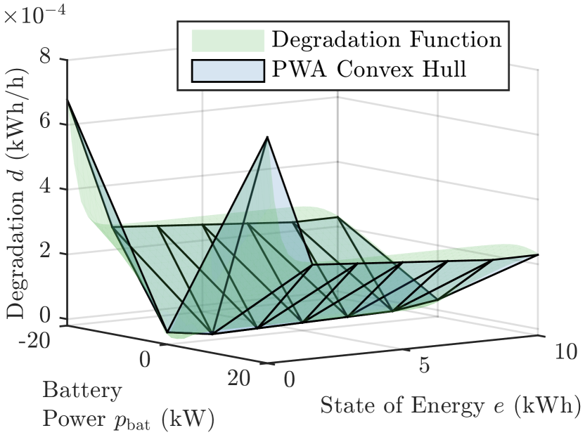
Battery degradation reduces the available battery capacity. It has an impact on the overall profitability, since the storage revenue decreases over time due to the capacity loss. There is a complex relationship between battery degradation and operational management, such that the operational strategy has an impact on lifetime and profitability. In [26], we presented a method to identify a stationary degradation process on an arbitrary battery usage pattern. The method produces a degradation map, where degradation is a function of the battery power and SoE. By using a convex PWA representation of the degradation map it is possible to account for degradation in the operational domain with efficient optimization solvers. As an illustrative example, we show a degradation map for a LiFePO4 system in Fig. 4. The green surface represents an empirical degradation function from [27] that we have scaled and transformed to the energy/power domain. The blue PWA map denotes its convex hull.

To calculate the total capacity fade per time $d$ e.g. in kWh/h as a function of the SoE $e$, battery power $p_{\mathrm{bat}}$, and energy capacity $z$, the PWA map for one battery system has the following structure

$$d=\max\left(\left[\boldsymbol{a}_{1}\ \boldsymbol{a}_{2}\ \boldsymbol{a}_{3}\right]\left[\begin{array}[h]{c}p_{\mathrm{bat}}\\ e\\ z\end{array}\right]\right)\quad,$$ (28)

where $\boldsymbol{a}_{1},\boldsymbol{a}_{2},\boldsymbol{a}_{3}\in\mathbb{R}^{n_{\mathrm{p}}}$ are parameters that span $n_{\mathrm{p}}$ planes in $\mathbb{R}^{3}$.

Figure 4: Illustration of a degradation map with an energy capacity of $z=$10kWh showing the incremental capacity loss as a function of the State of Energy (SoE) $e$ and applied battery power $p_{\mathrm{bat}}$. The red surface is the original degradation function from [27]. The blue piecewise-affine (PWA) map is its convex hull representation (28).

The incremental capacity loss for one battery system at time step $k$ can be included inside the optimal placement and sizing problem (11) by using the following epigraph formulation:

$$\boldsymbol{a}_{1}(p_{\mathrm{gen}}^{s,\mathrm{dis}}(k)+p_{\mathrm{gen}}^{s,\mathrm{ch}}(k))+\boldsymbol{a}_{2}e(k)+\boldsymbol{a}_{3}z\leq\boldsymbol{1}d(k)\quad,$$ (29)

where $p_{\mathrm{bat}}=p_{\mathrm{gen}}^{s,\mathrm{dis}}+p_{\mathrm{gen}}^{s,\mathrm{ch}}$. In the same straightforward way, we can account for battery degradation for multiple steps and battery systems, the following matrix definitions need to be included into the placement and sizing problem:

$$\boldsymbol{A}_{\mathrm{deg}}^{u}= [\boldsymbol{I}^{Nn_{\mathrm{s}}}\otimes\boldsymbol{a}_{1}][\boldsymbol{I}^{N}\otimes[\boldsymbol{I}^{n_{\mathrm{s}}}\boldsymbol{I}^{n_{\mathrm{s}}}]\boldsymbol{C}_{\mathrm{s}}]+[\boldsymbol{I}^{Nn_{\mathrm{s}}}\otimes\boldsymbol{a}_{2}]\boldsymbol{S}_{u}\ ,$$ (30)

$$\boldsymbol{A}_{\mathrm{deg}}^{z}= \boldsymbol{I}^{N}\otimes[\boldsymbol{I}^{n_{\mathrm{s}}}\otimes\boldsymbol{a}_{3}]\quad,$$ (31)

$$\boldsymbol{A}_{\mathrm{deg}}^{D}= \boldsymbol{I}^{Nn_{\mathrm{s}}}\otimes-\boldsymbol{1}^{n_{\mathrm{p}}\times 1}\quad,$$ (32)

$$\boldsymbol{b}_{\mathrm{deg}}= -[\boldsymbol{I}^{Nn_{\mathrm{s}}}\otimes\boldsymbol{a}_{2}]\boldsymbol{S}_{x}\boldsymbol{e}(0)\quad.$$ (33)

III-B5 Incorporation of PV generators (11f)

The PV predictions $\hat{\boldsymbol{p}}_{\mathrm{gen}}^{\mathrm{pv}}$ for $n_{\mathrm{pv}}$ PV generators can be included as time series into constraint (11f) by applying at each time step $k$

$$\hat{\boldsymbol{p}}_{\mathrm{gen}}^{\mathrm{pv}}(k)=\boldsymbol{C}_{\mathrm{pv}}\boldsymbol{x}_{\max,k}\quad,$$ (34)

where $\boldsymbol{C}_{\mathrm{pv}}\in\mathbb{R}^{n_{\mathrm{pv}}\times 2n_{\mathrm{l}}+2n_{\mathrm{g}}+n_{\mathrm{b}}}$ maps the PV generators to the optimization vector $\boldsymbol{x}_{k}$.

III-B6 Problem Complexity

The average polynomial running time of solving an LP problem with the Simplex method can be approximated according to [28] by

$$\mathcal{O}\left(n_{\mathrm{d}}^{3}n_{\mathrm{c}}^{1/(n_{\mathrm{d}}-1)}\right)\quad,$$ (35)

where $n_{\mathrm{d}}$ is the size of the decision variables and $n_{\mathrm{c}}$ denotes the number of constraints. Taking the specific problem structure into account, the complexity bound for solving the LP problem (11) can be calculated as

$$\mathcal{O}\left(n_{\mathrm{d}}^{3}\right),$$ (36)

where the size of $n_{\mathrm{d}}\approx N(3n_{\mathrm{g}}+2n_{\mathrm{l}}+n_{\mathrm{b}}+n_{\mathrm{s}})$. Here, it is assumed that for large $N$ the term $n_{\mathrm{c}}^{1/(n_{\mathrm{d}}-1)}\rightarrow 1$. This means that the computation time depends strongly on the investment horizon $N$.

III-C Benders Decomposition

Since the LP problem (11) is intractable for infinite control horizons, we try to decompose our placement and sizing problem with respect to time. By exploiting the LP property, we can decompose our problem using Benders decomposition. We use the same decomposition procedure and notation according to [29].

III-C1 Master Problem

According to [29] problem (11) has a decomposable structure, since $\boldsymbol{z}$ acts as the complicating variable. Hence, the problem can be split into a storage planning master problem and sequentially-solvable subproblems reflecting the operational strategy. The master problem is

$$\begin{array}[]{lll}J^{*}(J_{\mathrm{sub}}^{(l)},\boldsymbol{z}^{(l)},\boldsymbol{\lambda}_{\mathrm{s}}^{(l)})=&\lx@intercol\displaystyle\min_{\boldsymbol{z},\alpha}\ \boldsymbol{c}_{\mathrm{s}}^{T}\boldsymbol{z}+\alpha\hfil\lx@intercol\\ &\text{s.t.}\\ &\text{(a)}&J_{\mathrm{sub}}^{(l)}+{\boldsymbol{\lambda}_{\mathrm{s}}^{T}}^{(l)}(\boldsymbol{z}-\boldsymbol{z}^{(l)})\leq\alpha\\ &\text{(b)}&\alpha\geq\alpha_{\mathrm{down}}\\ &\text{(c)}&\boldsymbol{0}\leq\boldsymbol{z}\leq\boldsymbol{z}_{\mathrm{max}}\quad,\end{array}$$ (37)

where $l$ denotes the iteration of the master problem, $\alpha$ is a proxy for the subproblem costs, and the vector $\boldsymbol{\lambda}_{\mathrm{s}}$ is the weighted sum of the dual variables from the subproblems that are associated with the equalities in $\boldsymbol{z}$. The variable $J_{\mathrm{sub}}$ denotes the sum of the subproblem objective values. Constraint (37a) represents the Benders cut at stage $l$ and constraints (37b,c) specify the bounds of the optimization variables.

III-C2 Sequential Subproblems

To reflect an MPC strategy we split the constraints in (11) with regard to the MPC control horizon $H$ and to the partitions $\boldsymbol{X}=[\boldsymbol{x}^{[1]},\ldots,\boldsymbol{x}^{[n]}]^{T}$,$\boldsymbol{Y}=[\boldsymbol{y}^{[1]},\ldots,\boldsymbol{y}^{[n]}]^{T}$, and $\boldsymbol{D}=[\boldsymbol{d}^{[1]},\ldots,\boldsymbol{d}^{[n]}]^{T}$ by defining $\boldsymbol{A}^{[j]},\boldsymbol{b}^{[j]}$. The $j$-th coupled subproblem is defined as

$$\begin{array}[]{lll}{J^{*}}^{[j]}(\boldsymbol{e}(jc),\boldsymbol{z})=&\lx@intercol\underset{\boldsymbol{x}^{[j]},\boldsymbol{y}^{[j]},\boldsymbol{z},\boldsymbol{d}^{[j]}}{\min}\ T\left(\sum\limits_{k=0}^{H-1}\boldsymbol{1}^{T}\boldsymbol{y}^{[j]}(k)\right.\hfil\lx@intercol\\ &&\lx@intercol\hfil\left.+{\boldsymbol{c}^{[j]}_{\mathrm{d}}}^{T}\boldsymbol{d}^{[j]}(k)\right)\hfil\lx@intercol\\ &\text{s.t.}\\ &\text{(a)}&\boldsymbol{A}^{[j]}\left[\begin{array}[]{c}\boldsymbol{x}^{[j]}\\ \boldsymbol{y}^{[j]}\\ \boldsymbol{z}\\ \boldsymbol{d}^{[j]}\end{array}\right]\leq\boldsymbol{b}^{[j]}(\boldsymbol{e}(jc))\\ &\text{(b)}&\boldsymbol{z}=\boldsymbol{z}^{(l)}:\boldsymbol{\lambda}^{[j]}\quad,\end{array}$$ (38)

where $c$ denotes the update cycle of the subproblem recomputation. The coupling arises due to the fact that the actual SoE vector from the previous optimization cycle needs to be transferred to the consecutive subproblem as initial state input denoted by $\boldsymbol{e}(jc)$. This fact does not allow us to solve the subproblems in a parallel fashion. The number of subproblems $n$ depends on how often we rerun the optimization problems, which can be specified with the parameters $c$ and $N$. This is shown in Fig. 5, in which the control actions are applied to the system for $c$ steps, before the next optimization problem is solved. This is also referred to as RHC and can be regarded as a closed loop feedback applied to the system.

Figure 5: Sequence diagram of subproblem decomposition for a closed loop MPC strategy.

To account for this strategy, we need to assign the individual contribution of each subproblem within $c$ steps in terms of the objective value and the dual variables $\boldsymbol{\lambda}^{[j]}$ that are associated with the equality constraints (38b). This can be achieved by calculating a weighted sum of $\boldsymbol{\lambda}^{[j]}$ with

$$\boldsymbol{\lambda}_{\mathrm{s}}=\sum\limits_{j=1}^{n}\boldsymbol{\lambda}^{[j]}\frac{c}{H}\quad,$$ (39)

and determining the total objective value by

$$J_{\mathrm{sub}}=\sum\limits_{j=1}^{n}\sum\limits_{k=1}^{c}\ \boldsymbol{1}^{T}\boldsymbol{y}^{*[j]}(k)+{\boldsymbol{c}^{[j]}_{\mathrm{d}}}^{T}\boldsymbol{d}^{*[j]}(k)\quad,$$ (40)

where the total number of subproblems $n$ that have to be solved is

$$n=\frac{N}{c}\quad.$$ (41)

III-C3 Algorithm

With the aformentioned modifications we can solve the Benders decomposition in the same way as in [29]. Algorithm 1 specifies the needed steps.

1:$\boldsymbol{z}=\boldsymbol{0},\ \alpha_{\mathrm{down}}=-100000,\ l=1$

2:solve master problem (37)

3:              $[\boldsymbol{z}^{(l)},\alpha^{(l)}]=\arg\min J^{*}$ discarding (37a)

4:do

5:     if $(l>1)$ then

6:         calculate Benders cut (37a)

7:         solve master problem (37)

8:              $[\boldsymbol{z}^{(l)},\alpha^{(l)}]=\arg\min J^{*}(J_{\mathrm{sub}}^{(l-1)},\boldsymbol{z}^{(l-1)},\boldsymbol{\lambda}_{\mathrm{s}}^{(l-1)})$

9:     end if

10:     for $j\ =1\ :\ n$ do

11:         solve subproblem (38)

12:              $[\boldsymbol{x}^{[j]},\boldsymbol{z},\boldsymbol{d}^{[j]}]=\arg\min{J^{*}}^{[j]}(\boldsymbol{e}(jc),\boldsymbol{z})$

13:     end for

14:     calculate $\boldsymbol{\lambda}_{\mathrm{s}}$ with (39)

15:     calculate subproblem objective $J_{\mathrm{{sub}}}^{(l)}$ with (40)

16:     $Z_{\mathrm{up}}^{(l)}=J_{\mathrm{{sub}}}^{(l)}+\boldsymbol{c}_{\mathrm{s}}^{T}\boldsymbol{z}^{(l)}$

17:     $Z_{\mathrm{down}}^{(l)}=J_{\mathrm{{sub}}}^{(l)}+\alpha^{(l)}$

18:     $l=l+1$

19:while $\left|\frac{Z_{\mathrm{up}}^{(l)}-Z_{\mathrm{down}}^{(l)}}{Z_{\mathrm{down}}^{(l)}}\right|>\epsilon$

Algorithm 1 Benders decomposition algorithm for optimal sizing and placement of distributed storage.

Note that the only difference from [29] is that we have to solve the subproblems sequentially instead of in parallel.

III-C4 Problem Complexity

We can also define a complexity bound for the decomposed problem (Alg. 1). It can be approximated by adding up the runtimes of the subproblems (38) as follows:

$$\mathcal{O}\left(lnH^{3}(3n_{\mathrm{g}}+2n_{\mathrm{l}}+n_{\mathrm{b}}+n_{\mathrm{s}})^{3}\right)\quad.$$ (42)

This means, if we consider $n=N/H$ subproblems, we can achieve an acceleration by factor of $N^{2}/(lH^{2})$ as compared to the problem (11).

IV Results

Here, we aim to define a realistic case study that assesses the economic value of different storage control strategies.

IV-A Test Case

As depicted in Fig. 6 we assume the LV CIGRE benchmark grid [30] as a realistic reference. The grid parameters are shown in Table I. As listed in Table II we configure the grid with a high PV penetration assuming that we can exploit the full roof top area of a single household. We compute the optimal locations and sizes of the batteries for different MPC controller strategies comprising different horizon lengths using the same input data for PV irradiation and load consumption. The controller objective is to minimize the generation costs at the feeder for a typical tariff scenario (day/night tariff [31] and feed-in tariff [32]) in Switzerland indicated with the cost parameters $c_{1}^{\mathrm{net}},c_{2}^{\mathrm{net}}$ and $c_{1}^{\mathrm{pv}}$. With this formulation we ensure that the group of prosumers gets rewarded for PV export and minimizes the consumption costs from the feeder by exploiting price differences of the tariff scheme and shifting energy from day to night through storage usage. In this way, the controller tries to utilize best the PV potential. We compute the placement and sizing problem for our simulation scenarios on the basis of just one full year to include the influence on seasonality, but also to save computation time. Therefore, $\boldsymbol{c}_{\mathrm{s}}$ represents the equivalent annual battery costs. In this regard we assume that the battery’s calendar lifetime is at maximum 10 years.

Figure 6: Local control area with group of prosumers (PV, battery systems and loads) populated on the CIGRE test grid from [30]. The cables indicated with red lines have a higher resistance (2.05$\Omega$/km) than the black ones (0.405$\Omega$/km).

Table I: Line setup of the CIGRE test grid.

Start node	End node	Resistance $R^{\prime}$ [$\Omega$/km]	Reactance $X^{\prime}_{L}$ [$\Omega$/km]	Length $l$ [m]	Max current $I_{\mathrm{max}}$ [A]
R1	R2	0.405	0.205	35	398
R2	R3	0.405	0.205	35	398
R3	R4	0.405	0.205	35	398
R4	R5	0.405	0.205	35	398
R5	R6	0.405	0.205	35	398
R6	R7	0.405	0.205	35	398
R7	R8	0.405	0.205	35	398
R8	R9	0.405	0.205	35	398
R9	R10	0.405	0.205	35	398
R3	R11	2.05	0.212	35	158
R4	R12	2.05	0.212	30	158
R12	R13	2.05	0.212	35	158
R13	R14	2.05	0.212	35	158
R14	R15	2.05	0.212	35	158
R6	R16	2.05	0.212	30	158
R9	R17	2.05	0.212	30	158
R10	R18	2.05	0.212	30	158

Table II: Simulation parameters.

Storage units	18
Storage power	$p_{\mathrm{gen}}^{\mathrm{s,max}}=$10kW, $q_{\mathrm{gen}}^{\mathrm{s,max}}=$ 10kVar
	rect. bounded
Storage efficiency	$\eta_{\mathrm{dis}}$ = 0.88, $\eta_{\mathrm{ch}}$= 0.88
Degradation model	LiFePO4 convexified
	degradation map from [27]
Prediction horizon $H$	6h, 12h, 24h (1d), 168h (1w), 672h (1m)
Update cycle $c$	6h
Sample time $T$	1h
Feed-in tariff $c_{1}^{\mathrm{net}}:p_{\mathrm{gen}}^{\mathrm{net}}<0$	50 €/MWh averaged from [32]
Net power cost $c_{2}^{\mathrm{net}}:p_{\mathrm{gen}}^{\mathrm{net}}\geq 0$	246 €/MWh 6:00-22:00 (Mon-Sat) [31]
	131.5 €/MWh rest of time
$\epsilon$ criterion	0.01
Battery cost $c_{\mathrm{d}}$	50-1000 €/kWh
PV units	18
PV power	$p_{\mathrm{gen}}^{\mathrm{pv,max}}$= 20 kW,
	$q_{\mathrm{gen}}^{\mathrm{pv,max}}$ = 10kVar, rect. bounded
PV profiles	radiation profiles for the year 2015
	and the city of Zurich
PV gen cost $c_{1}^{\mathrm{pv}}$	0 €/MWh
Storage gen cost $c_{1}^{\mathrm{s}}$	0 €/MWh
Total PV production	465 MWh
Total load consumption	61.5 MWh
Simulation horizon $N$	8760 (1 year)
Households	18 @ 4kWp generated
	load profiles from [33]
Grid	European LV network [30]
Voltage limits	$v_{\mathrm{max}}=1.1$,$v_{\mathrm{min}}=0.9$
Thermal limits	according to [30]

Figure 7: Optimal placement and sizing results of the installed distributed battery storage as a function of the battery investment cost and control horizon $H$. The height of the bars represent the storage size, while the battery locations correspond to the nodes referenced in Fig. 6. The control horizon $H$ also corresponds to hours.

IV-B Heuristic Controller

To compare our enhanced predictive storage control strategy, we modify a standard heuristic control strategy that is described in [34, 35]. In particular, we consider the storage control strategy from [34] that has a fixed feed-in limitation. The authors of [35] refer to this mode as a conventional storage strategy. This rule-based controller does not include any forecast of the PV production and is therefore a non-predictive controller. It stores surplus PV power during the day and curtails PV power when the batteries are full and the grid limit is exceeded. In contrast to [34] and with the aim to utilize more PV power, we force the batteries to empty in the morning in cases when the available energy content was not consumed by the household over night. In addition, we determine dynamically the grid limits by running an AC Optimal Power Flow (AC-OPF). The AC-OPF framework allows us to also consider optimal RPC and APC.

Unfortunately, we cannot formulate an optimal placement and sizing problem using the proposed Benders decomposition technique, since this strategy does not provide any dual variables to reduce the space of feasible solutions by Benders cuts. However, to compare the strategies, we run the heuristic strategy with the optimal storage configuration that is obtained by the MPC strategy.

IV-C Convergence and Computation Time

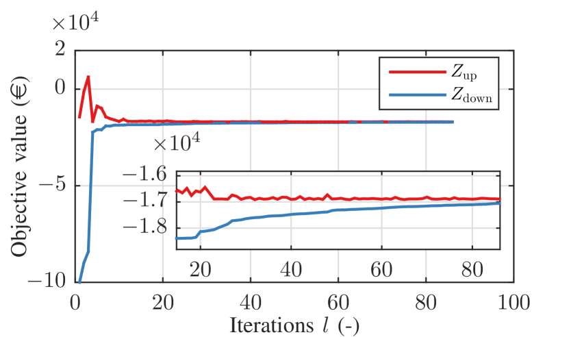
Figure 8 shows the typical convergence rate of our proposed Benders decomposition approach for one simulation scenario. A simulation scenario is defined as a full-year simulation ($N$=8760) at a given control horizon $H$ and a fixed battery cost level. One can observe that around 80 iterations are needed to reach the $\epsilon$-criterion specified in Alg. 1. The computation time ranges from 24 hours ($H=24$) to 3 days ($H=672$) to sequentially solve one simulation scenario with the CPLEX LP solver [36]. Instead of solving all 30 simulation scenarios consecutively, we run multiple simulation scenarios in a parallel fashion on multi-core processors to save computation time.

Figure 8: Typical convergence rate of the proposed Benders decomposition algorithm.

IV-D Sizing and Placement

First, we run the sizing and placement problem without the degradation model in the MPC strategy to further save computation time. Figure 7 shows the results of the optimal DBS distribution as a function of different control horizons and battery costs. The highest line loading we observe is at line R1-R2. The largest storage sizes are placed at the nodes R12-R15 and R9 to support the line R1-R2. The placement decisions for R12-R15 are associated with lines that have a higher resistance. Also the resistance from the feeder to the node R9 is higher due to a longer cable length. This means that with this configuration we can reduce the network losses most effectively and therefore utilize more PV power.

Figure 9 shows the aggregated placed storage size as a function of the battery cost. One can see that when decreasing the horizon length, less storage capacity is placed. In addition, at a cost level of 1000€/kWh it is not viable any longer to place storage in the grid. It is noteworthy that the storage size is almost the same, whether operating the storage at daily ($H=24$), weekly ($H=168$) or monthly ($H=672$) control horizons.

Figure 9: Aggregated storage size as a function of the battery cost for different control horizons.

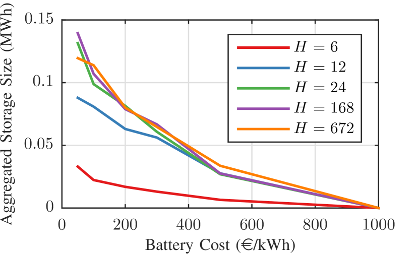
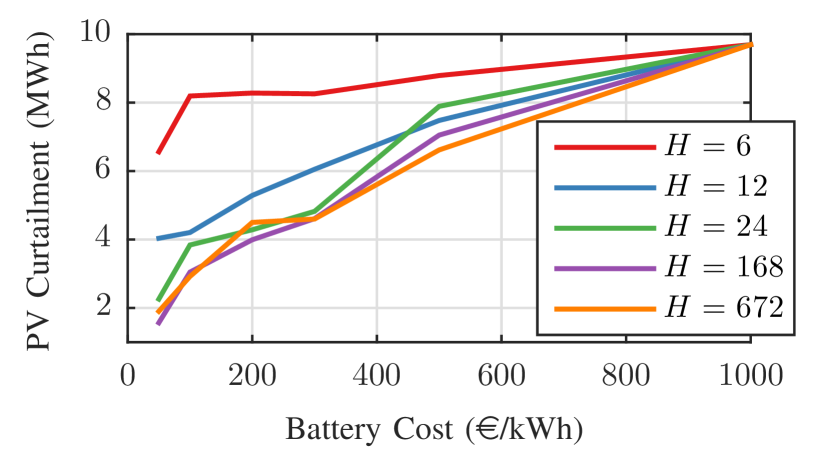
Fig. 10 shows the PV curtailment as a function of the battery cost for the different control horizons. One can observe that the curtailment levels are higher, when using sub-daily horizons. By using longer horizons ($H=24,168,672$) the PV curtailment is reduced by about half, since the aggregated storage size is higher for these controller strategies (see Fig. 9).

Figure 10: Total PV curtailment as a function of the battery cost for different control horizons.

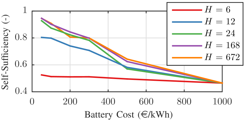
However, despite of the same storage size, the degree of self-sufficiency of the local control area for the horizon strategies ($H=168,672$) is in almost all cases higher (see Fig.11). It can be anticipated that the economic benefit of shifting energy over weekly or monthly intervals to cover the loads is not significant for the considered battery cost levels. This means that the driving factor for sizing is the mitigation of PV curtailment on daily patterns, such that the optimal size is determined by finding the best compromise between minimizing PV curtailment and battery investment. This is also the reason why we observe a saturation in storage size for multi-day horizons, since the storage size is already large enough to increase the self-sufficiency. The degree of self-sufficiency describes to which extent the local control area is independent of the grid. It is defined as

$$\text{self-sufficiency}=\frac{E_{\mathrm{ld}}-E_{\mathrm{net}}^{\mathrm{im}}}{E_{\mathrm{ld}}}\quad,$$ (43)

where $E_{\mathrm{ld}}$ is the yearly energy consumption of all loads and $E_{\mathrm{net}}^{\mathrm{im}}$ is the yearly imported energy from the feeder. A factor of one would mean that the control area is off-the-grid.

Figure 11: Self-sufficiency of the control area as a function of the battery cost for different control horizons.

IV-E Economic Value of Horizon Length

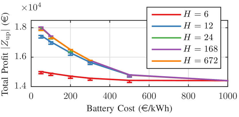
Next, we aim to compare the impact on the investment profit for different control horizon lengths. Figure 12 shows the investment profit corresponding to the objective value of (37) as a function of the battery cost for different control horizons. One can observe that sub-daily horizon strategies are less profitable than daily, weekly or monthly horizon strategies. Another interesting result is that multi-day horizons perform similarly, which means that longer control horizons than one day do not further improve the profit.

Figure 12: Yearly investment profit as a function of the battery cost for different control horizons.

IV-F Economic Assessment

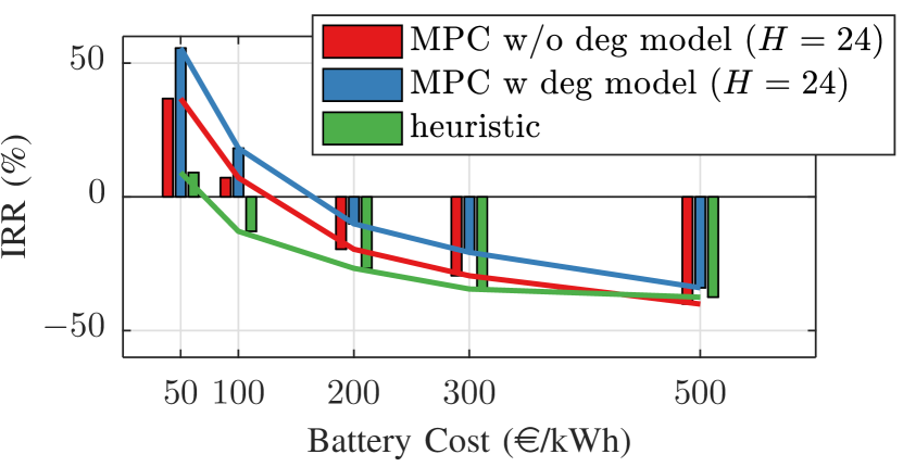
For the economic assessment, we compare the MPC strategies with and without degradation model for a 24 hour horizon with the heuristic storage control strategy. By using the degradation map (28), we first compute the battery lifetime in $m$ years for the different strategies according to the End of Life (EoL) criterion of 0.8. Here, the EoL defines the aggregated remaining capacity in the given control area after $m$ years. This allows us to assume that the expected revenue streams over the years are approximately the same. Figure 13 shows the battery lifetimes for the type of different storage control strategies.

Figure 13: Battery lifetime as a function of the battery cost for different storage control strategies for an EoL criterion 0.8. Note that no battery capacity is installed for the battery cost of 1000€/kWh.

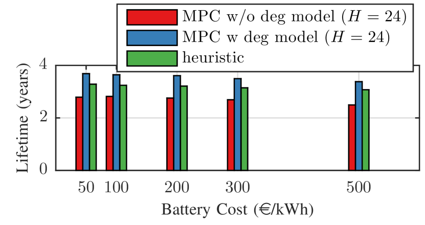
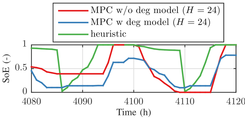
It can be inferred that the storage control strategy has a great impact on battery lifetime. This can be explained by Fig. 14 that shows the resulting evolution of the SoE trajectories from the different controllers. While the MPC with degradation model avoids SoE regimes that are associated with high battery wear, the other ones idle the batteries at low SoE regimes or use the full capacity potential.

Figure 14: Resulting state of energy (SoE) trajectories from different storage control strategies.

The variable $-J_{\mathrm{sub}}$ can be regarded as the revenue stream for one year. To account only for the storage investment, we need to define the revenue difference considering an investment with (wS) and without storage (w/oS). The Net Present Value (NPV) of the investment is

$$\text{NPV}=-\boldsymbol{c}_{\mathrm{d}}^{T}\boldsymbol{z}+\sum\limits_{k=1}^{m}\frac{-J_{\mathrm{sub}}^{\text{wS}}+J_{\mathrm{sub}}^{\text{w/oS}}}{(1+\text{IRR})^{k}}\quad.$$ (44)

To obtain a viable investment the NPV has to be greater than zero. Since the Internal Rate of Return (IRR) is a direct measure for the Return on Investment (ROI), we solve (44) for the IRR by setting the NPV to zero.

Although the battery lifetime is longer for the heuristic controller as compared to the MPC strategy without degradation model, the IRRs for the MPC strategies are superior, which are shown in Fig. 15. When using MPC strategies the group of prosumers gets viable results below battery cost levels of $\approx$175€/kWh (w deg model) and $\approx$125€/kWh (w/o deg model), while the heuristic strategy only achieves a profit below $\approx$60€/kWh. This is due to the fact that the MPC strategies can generate more value by using forecast information and therefore better utilize the batteries.

Figure 15: Internal Rate of Return (IRR) as a function of the battery cost for different storage control strategies.

V Conclusion

This paper presents a novel Benders decomposition method that considers MPC strategies in a planning and operation problem. We split the sizing and placement problem into a master planning problem and sequentially-solvable subproblems reflecting a predictive storage control strategy. The storage control strategy is formulated as an MPC strategy that optimally schedules distributed battery storage to maximize PV self-sufficiency and PV utilization while considering grid constraints and minimizing battery degradation. The grid constraints are incorporated as a multi-period OPF problem using an existing linearized version of the OPF. Due to the linear property of the placement and sizing problem, it can be decomposed by using Benders decomposition.

From the case study it can be concluded that MPC strategies are in general more profitable than heuristic controller strategies and are viable for battery costs below 175€/kWh. The horizon length has a great impact on profitability. Control horizons that are shorter than 24 hours limit the revenue potential, while operating storage on a daily base is as good as on a weekly or monthly base in terms of the overall profitability. Nevertheless, higher horizon lengths increase the degree of self-sufficiency of the control area. The main conclusion on the optimal sizing and placement of DBS is that the best scheme is achieved when overloaded network elements are supported and network losses are reduced. As a further finding, by using a battery degradation model within our MPC controllers, we can extend the battery lifetime and hence further increase the total profitability of the group of prosumers.

Future work relates to further analyze the impact of different PV installations and network topologies on the optimal placement and sizing of DBS. In this regard, it could also be studied whether centralized or distributed battery storage configurations are more preferable.

References

- [1] F. J. de Sisternes, J. D. Jenkins, and A. Botterud, “The value of energy storage in decarbonizing the electricity sector,” Applied Energy, vol. 175, pp. 368–379, 2016.
- [2] R. Sims et al, Integration of Renewable Energy into Present and Future Energy Systems, ser. IPCC Special Report on Renewable Energy Sources and Climate Change Mitigation. Cambridge University Press, 2011.
- [3] K. C. Divya and J. Ostergaard, “Battery energy storage technology for power systems - An overview,” Electric Power Systems Research, vol. 79, no. 4, pp. 511–520, 2009.
- [4] Bundesnetzagentur, “Installierte EE-Leistung zum 31.12.2015.” [Online]. Available: http://www.bundesnetzagentur.de/SharedDocs/Downloads/DE/Sachgebiete/Energie/Unternehmen_Institutionen/ErneuerbareEnergien/ZahlenDatenInformationen/InstallierteLeistung_2015_BF.pdf?__blob=publicationFile&v=4
- [5] S. Wogrin and D. F. Gayme, “Optimizing storage siting, sizing, and technology portfolios in transmission-constrained networks,” IEEE Transactions on Power Systems, vol. 30, no. 6, pp. 3304–3313, 2015.
- [6] B. Xu, A. Ulbig, and G. Andersson, “Impacts of dynamic line rating on power dispatch performance and grid integration of renewable energy sources,” in Innovative Smart Grid Technologies Europe (ISGT EUROPE), 2013 4th IEEE/PES. IEEE, 2013.
- [7] M. R. Almassalkhi and I. A. Hiskens, “Model-predictive cascade mitigation in electric power systems with storage and renewables? part i: Theory and implementation,” IEEE Transactions on Power Systems, vol. 30, no. 1, pp. 67–77, 2015.
- [8] E. Camponogara, D. Jia, B. H. Krogh, and S. Talukdar, “Distributed model predictive control,” IEEE Control Systems, vol. 22, no. 1, pp. 44–52, 2002.
- [9] A. N. Venkat, I. A. Hiskens, J. B. Rawlings, and S. J. Wright, “Distributed MPC strategies with application to power system automatic generation control,” IEEE transactions on control systems technology, vol. 16, no. 6, pp. 1192–1206, 2008.
- [10] A. Ulbig, “Operational flexibility in electric power systems,” Ph.D. dissertation, ETH Zurich, 2014.
- [11] P. Denholm, J. Jorgenson, T. Jenkin, D. Palchak, B. Kirby, M. O. Malley, M. Hummon, and O. Ma, “The value of energy storage for grid applications,” National Renewable Energy Laboratory (NREL), Tech. Rep. NREL/TP-6A20-58465, 2013. [Online]. Available: http://www.nrel.gov/docs/fy13osti/58465.pdf
- [12] P. Harsha and M. Dahleh, “Optimal sizing of energy storage for efficient integration of renewable energy,” IEEE Conference on Decision and Control and European Control Conference, pp. 5813–5819, 2011.
- [13] ——, “Optimal management and sizing of energy storage under dynamic pricing for the efficient integration of renewable energy,” IEEE Transactions on Power Systems, vol. 30, no. 3, pp. 1164–1181, 2014.
- [14] H. Pandzic, Y. Wang, T. Qiu, Y. Dvorkin, and D. S. Kirschen, “Near-optimal method for siting and sizing of distributed storage in a transmission network,” IEEE Transactions on Power Systems, vol. 30, no. 5, pp. 2288–2300, 2015.
- [15] C. Thrampoulidis, S. Bose, and B. Hassibi, “Optimal placement of distributed energy storage in power networks,” IEEE Transactions on Automatic Control, vol. 61, no. 2, pp. 416–429, 2016.
- [16] Y. M. Atwa and E. F. El-Saadany, “Optimal allocation of ESS in distribution systems with a high penetration of wind energy,” IEEE Transactions on Power Systems, vol. 25, no. 4, pp. 1815–1822, 2010.
- [17] A. Castillo and D. F. Gayme, “Profit maximizing storage allocation in power grids,” Proceedings of the IEEE Conference on Decision and Control, pp. 429–435, 2013.
- [18] S. Bose, D. F. Gayme, U. Topcu, and K. M. Chandy, “Optimal placement of energy storage in the grid,” Proceedings of the IEEE Conference on Decision and Control, pp. 5605–5612, 2012.
- [19] K. Dvijotham, M. Chertkov, and S. Backhaus, “Storage sizing and placement through operational and uncertainty-aware simulations,” Proceedings of the Annual Hawaii International Conference on System Sciences, pp. 2408–2416, 2014.
- [20] E. Nasrolahpour, S. J. Kazempour, H. Zareipour, and W. D. Rosehart, “Strategic sizing of energy storage facilities in electricity markets,” IEEE Transactions on Sustainable Energy, vol. 7, no. 4, pp. 1462–1472, 2016.
- [21] M. Nick, R. Cherkaoui, and M. Paolone, “Optimal siting and sizing of distributed energy storage systems via alternating direction method of multipliers,” International Journal of Electrical Power and Energy Systems, vol. 72, pp. 33–39, 2015. [Online]. Available: http://dx.doi.org/10.1016/j.ijepes.2015.02.008
- [22] P. Fortenbacher, M. Zellner, and G. Andersson, “Optimal sizing and placement of distributed storage in low voltage networks,” in 19th Power Systems Computation Conference, Genova, Italy, 2016. [Online]. Available: http://arxiv.org/abs/1512.01218
- [23] L. Baringo and A. J. Conejo, “Wind power investment: A Benders decomposition approach,” IEEE Transactions on Power Systems, vol. 27, no. 1, pp. 433–441, 2012.
- [24] J.-H. Teng, “A direct approach for distribution system load flow solutions,” IEEE Transactions on Power Delivery, vol. 18, no. 3, pp. 882–887, July 2003.
- [25] P. Fortenbacher, J. Mathieu, and G. Andersson, “Optimal real-time control of multiple battery sets for power system applications,” in Proceedings of POWERTECH, 2015.
- [26] ——, “Modeling, identification, and optimal control of batteries for power system applications,” in Proceedings of the Power Systems Computation Conference, 2014.
- [27] J. C. Forman, S. J. Moura, J. L. Stein, and H. K. Fathy, “Optimal Experimental Design for Modeling Battery Degradation,” in Proceedings of ASME Dynamic Systems and Control Conference, vol. 1, 2012, pp. 309–318.
- [28] A. Schrijver, Theory of Linear and Integer Programming, ser. Wiley Series in Discrete Mathematics & Optimization. John Wiley & Sons, 1998.
- [29] A. Conejo, E. Castillo, R. Mínguez, and R. García-Bertrand, Decomposition techniques in mathematical programming. Springer, 2006.
- [30] “Benchmark systems for network integration of renewable and distributed energy resources,” Cigre Task Force C6.04.02, Tech. Rep., 2014. [Online]. Available: http://c6.cigre.org/Publications/Technical-Brochures
- [31] “Tariff scheme of the city Zurich for private households,” Utility of the city Zurich, Zurich, Tech. Rep., 2016. [Online]. Available: https://www.ewz.ch/content/dam/ewz/services/dokumentencenter/energie-beziehen/dokumente/gruener-strom-fuer-mein-zuhause/stromtarif-2016-zh-private.pdf
- [32] “Feed in tariff of the city Zurich,” Utility of the city Zurich, Zurich, Tech. Rep., 2016. [Online]. Available: https://www.ewz.ch/content/dam/ewz/services/dokumentencenter/energie-produzieren/dokumente/verguetung-stromruecklieferung-zh-2016-17.pdf
- [33] C. Bucher and G. Andersson, “Generation of domestic load profiles - an adaptive top-down approach,” in Proceedings of PMAPS 2012, Istanbul, Turkey, June 2012.
- [34] J. Weniger, J. Bergner, and V. Quaschning, “Integration of PV power and load forecasts into the operation of residential PV battery systems,” in 4th Solar Integration Workshop, 2014, pp. 383–390. [Online]. Available: https://pvspeicher.htw-berlin.de/wp-content/uploads/2014/04/SIW-2014-Integration-of-PV-power-and-load-forecasts-into-the-operation-of-residential-PV-battery-systems.pdf
- [35] F. Marra, G. Yang, C. Træholt, J. Østergaard, and E. Larsen, “A decentralized storage strategy for residential feeders with photovoltaics,” IEEE Transactions on Smart Grid, vol. 5, no. 2, pp. 974–981, 2014.
-
[36]
“IBM ILOG CPLEX v12.1 user’s manual for CPLEX,” cplex, Tech. Rep., 2009.
[Online]. Available:
ftp://public.dhe.ibm.com/software
/websphere/ilog/docs/optimization/cplex/ps_usrmancplex.pdf