A fully diagonalized spectral method using generalized Laguerre functions on the half line
Abstract.
A fully diagonalized spectral method using generalized Laguerre functions is proposed and analyzed for solving elliptic equations on the half line. We first define the generalized Laguerre functions which are complete and mutually orthogonal with respect to an equivalent Sobolev inner product. Then the Fourier-like Sobolev orthogonal basis functions are constructed for the diagonalized Laguerre spectral method of elliptic equations. Besides, a unified orthogonal Laguerre projection is established for various elliptic equations. On the basis of this orthogonal Laguerre projection, we obtain optimal error estimates of the fully diagonalized Laguerre spectral method for both Dirichlet and Robin boundary value problems. Finally, numerical experiments, which are in agreement with the theoretical analysis, demonstrate the effectiveness and the spectral accuracy of our diagonalized method.
Key words and phrases:
Spectral method, Sobolev orthogonal Laguerre functions, elliptic boundary value problems, error estimates.2000 Mathematics Subject Classification:
76M22, 33C45, 35J25, 65L701. Introduction
Spectral methods for solving partial differential equations on unbounded domains have gained a rapid development during the last few decades. An abundance of literature on this research topic has emerged, and their underlying approximation approaches can be essentially classified into three catalogues [4, 27]:
- (i)
-
(ii)
map the original problem on an unbounded domain to one on a bounded domain and use classic spectral methods to solve the new problem [9]; or equivalently, approximate the original problem by some non-classical functions mapped from the classic orthogonal polynomials/functions on a bounded domain [2, 3, 7, 11, 12, 27, 31, 34];
- (iii)
The third approach is of particular interest to researchers, and has won an increasing popularity in a broad class of applications, owing to its essential advantages over other two approaches. These direct approximation schemes constitute an initial step towards the efficient spectral methods, which admit fast and stable algorithms for their efficient implementations.
As we know, the Fourier spectral method makes use of the eigenfunctions of the Laplace operator which are orthogonal to each other with respect to the Sobolev inner product involving derivatives, thus the corresponding algebraic system is diagonal [4, 5, 25]. This fact together with the availability of the fast Fourier transform (FFT) makes the Fourier spectral method be an ideal approximation approach for differential equations with periodic boundary conditions. Although the utilization of the genuine orthogonal polynomials/functions in this direct approach usually leads to a highly sparse (e.g., tri-diagonal, penta-diagonal) and well-conditioned algebraic system, however, in many cases, people still want to get a set of Fourier-like basis functions for a fully diagonalized algebraic system [28].
The main purpose of this paper is to construct the Fourier-like Sobolev orthogonal basis functions [8, 21] for elliptic boundary value problems on the half line . For this purpose, we shall first extend the definition of Laguerre polynomials and Laguerre functions for to allow being any real number. The resulting generalized Laguerre functions are proven to be the eigenfunctions of certain high order Sturm-Liouville differential operators (see Lemma 2.6 of this paper). Moreover, they are complete and mutually orthogonal in for any nonnegative integer with respect to an equivalent Sobolev inner product (see (2.23) of this paper).
Since the problem is dependent on the inner product originated from the coercive bilinear form of the elliptic equation, it does not necessarily coincide with the equivalent Sobolev inner product, further efforts should be paid to obtain the Fourier-like basis functions for a fully diagonalized spectral approximation, in spite of the Sobolev orthogonality of . Starting with , stable and efficient algorithms are then proposed to construct the Fourier-like basis functions for the non-homogeneous Dirichlet and Robin boundary value problems of the second order elliptic equations. In the sequel, both the exact solution and the approximate solution can be represented as infinite and truncated Fourier series in , respectively. Although the fully diagonalized spectral methods are studied for second order equations, they can be readily generalized to solve -th order equations by starting with .
An ideal spectral approximation to differential equations may guarantee an optimal error estimate in its convergence analysis. To match this requirement, various orthogonal projections involving different orders of derivatives and boundary conditions have been designed and studied case by case, which frequently make the numerical analysis in spectral method a tedious task. Moreover, the traditional routine to measure the approximation error is first to establish the norm defined by a second-order self-adjoint differential operator, and then estimate the upper bound of the approximation error with the induced norms. However, this practical approach usually fails to characterize the function space in which the orthogonal projection has an optimal error estimate.
To conquer these difficulties, we need a unified definition of the orthogonal spectral projections with a systematic numerical analysis. Fortunately, the Sobolev orthogonality of the generalized Laguerre functions with a negative integer enables us to define the unified orthogonal projection from to the finite approximation space for all nonnegative integer , ignoring the specific value of . More importantly, such an orthogonal projection interpolates the endpoint function values up to the -th derivative, i.e, for any and . This endpoint interpolation property ensures , thus makes applicable to both the Dirichlet and Robin boundary value problems, and available to multi-domain spectral methods. Besides, owing to the clarity of the orthogonality structure of the generalised Laguerre functions, one can not only derive an optimal order of the convergence for the approximated function, but also get a generic characterization of the function space where the orthogonal projection has an optimal error estimate.
Therefore, the second purpose of this paper is to establish such a unified orthogonal Laguerre projection, and apply it to the convergence analysis on the fully diagonalized Laguerre spectral method for both the Dirichlet and Robin boundary value problems of second order elliptic equations.
The remainder of the paper is organized as follows. In Section 2, we first make conventions on the frequently used notations, and then introduce generalized Laguerre polynomials and functions with arbitrary index . The fully diagonalized Laguerre spectral methods and the implementation of algorithms are proposed in Section 3 for the Dirichlet and Robin boundary value problems of second order elliptic equations. Section 4 is then devoted to the convergence analysis of the unified orthogonal projection together with our Laguerre spectral methods. Finally, numerical results are presented in Section 5 to demonstrate the effectiveness and accuracy of the proposed diagonalized Laguerre spectral methods, which are in agreement with our theoretical predictions.
2. Generalized Laguerre polynomials and functions
2.1. Notations and preliminaries
Let and be a weight function which is not necessary in . We define
with the following inner product and norm,
For simplicity, we denote and For any integer , we define
with the following semi-norm and norm,
For any real we define the space and its norm by function space interpolation as in [1]. In cases where no confusion arises, may be dropped from the notations whenever Specifically, we shall use the weight functions and in the subsequent sections.
We denote by the collection of real numbers, by and the collections of nonnegative and negative integers, respectively. Further, we let be the space of polynomials of degree .
Let . We also define the characteristic functions for ,
For short we write .
2.2. Generalized Laguerre polynomials
It is well known that, for the classical Laguerre polynomials admit an explicit representation (see [29]):
| (2.1) |
where we use the Pochhammer symbol for any and .
The classical Laguerre polynomials can be extended to cases with any and the same representation as (2.1), which are referred to as the generalized Laguerre polynomials (cf. [23]). Obviously, the generalized Laguerre polynomials constitute a complete basis for the linear space of real polynomials as well, since for all .
The generalized Laguerre polynomials fulfill the following recurrence relations.
Lemma 2.1.
For any , it holds
| (2.2) |
Proof.
The recurrence relation (2.2) for can be derived from those of the classic Laguerre polynomials for by the continuation method. Here, we also give a concrete proof by the representation (2.1). Using the expression (2.1), we obtain that for integer
Then a direct computation shows that
The desired result is now derived. ∎
Lemma 2.2.
For any and , it holds
| (2.3) | ||||
| (2.4) | ||||
| (2.5) | ||||
| (2.6) |
where for any
Proof.
Lemma 2.3.
For any , the generalized Laguerre polynomials satisfy the Sturm-Liouville equation
| (2.7) |
or equivalently,
| (2.8) |
with the corresponding eigenvalue .
Proof.
We are interested in those generalized Laguerre polynomials with an integer index .
Lemma 2.4.
For any , we have
| (2.9) |
And for any , the following orthogonality relation holds:
| (2.10) |
where is the Kronecker symbol.
Proof.
We now conclude this subsection with some generalized Laguerre polynomials for .
2.3. Generalized Laguerre functions
In this subsection, we shall introduce the generalized Laguerre functions with arbitrary parameters and and present some properties.
The generalized Laguerre functions are defined by
| (2.11) |
and the multiplication of and the leading term of is simply referred to as the leading term of .
According to (2.9), for any , we have
| (2.12) |
which means that is a zero of with the multiplicity , i.e.,
| (2.13) |
Lemma 2.5.
For any , it holds that
| (2.14) | ||||
| (2.15) | ||||
| (2.16) | ||||
| (2.17) | ||||
| (2.18) | ||||
Hereafter, we use the convention that whenever .
The generalized Laguerre functions are eigenfunctions of certain singular Sturm-Liouville differential operators.
Lemma 2.6.
For any , it holds that
| (2.19) |
where satisfies the following recurrence relation,
| (2.20) |
Proof.
For any , and , define the bilinear form on ,
| (2.21) |
It is obvious that is an inner product on if .
Theorem 2.1.
The generalized Laguerre functions for are mutually orthogonal with respect to the weight function ,
| (2.22) |
More generally, for any and ,
| (2.23) |
where the positive numbers satisfy the recurrence relation
| (2.24) |
under the convention that whenever .
Proof.
The orthogonality (2.22) is an immediate consequence of (2.10). Meanwhile, the recursive formula (2.21) of binomial coefficients together with (2.15) and (2.16) yields
| (2.25) | ||||
The normalization constants and the eigenvalues are closely related. In effect, for any , , we get that
| (2.27) | ||||
where the third inequality sign is obtained by integration by parts combined with (2.13).
Moreover, for sufficiently large , an induction procedure starting with (2.20) reveals
| (2.28) |
which implies
| (2.29) |
The following eigenvalues and normalization constants are of our particular interest,
| (2.30) | ||||
| (2.31) |
3. Fully diagonalized spectral methods
In this section, we propose the fully diagonalized spectral methods using generalized Laguerre functions for solving differential equations on the half line. The main idea is to find a system of Sobolev orthogonal functions [8, 21] with respect to the coercive bilinear form arising from differential equation, such that both the exact solution and the approximate solution can be explicitly expressed as a Fourier series in the Sobolev orthogonal functions. Although we only consider in this section non-homogenous Robin/Drichlet boundary value problems of a second order equation, one can extend the fully diagonalized spectral methods for solving partial differential equations of an arbitrary high order.
3.1. Robin boundary value problems
Consider the second order elliptic boundary value problem:
| (3.1) |
A weak formulation of (3.1) is to find such that
| (3.2) |
The Lax-Milgram lemma guarantees a unique solution to (3.2) if .
For an efficient approximation scheme, one usually chooses the generalized Laguerre functions as the basis functions for problem (3.3). However, we are eager for an ideal approximation scheme whose (total) stiff matrix, in analogue to the Fourier spectral method for periodic problem, is diagonal. Obviously, the utilization of the basis functions leads to a tridiagonal algebraic system. To this end, we shall construct new basis functions which are mutually orthogonal with respect to the Sobolev inner product instead of defined in Theorem 2.1.
Lemma 3.1.
Let be the Sobolev orthogonal Laguerre functions such that and
| (3.4) |
Then satisfy the following recurrence relation,
| (3.5) |
where and
Proof.
By the orthogonality assumption (3.4) of ,
Meanwhile, by (3.2) and (2.21), for any ,
Both the first and the second terms in the righthand side above are zero due to the orthogonality relation (2.23) of and the homogeneity boundary condition (2.13) for . Further by (2.15) and the orthogonality relation (2.22) for ,
which, in return, implies
3.2. Dirichlet boundary value problems
Consider the second order elliptic boundary value problem:
| (3.6) |
A weak formulation of (3.6) is to find such that and
| (3.7) |
Clearly, if , then by Lax-Milgram lemma, (3.7) admits a unique solution.
To propose a fully diagonal approximation scheme for (3.7) , we need to construct new basis functions which are mutually orthogonal with respect to the Sobolev inner product .
Lemma 3.2.
Let be the Sobolev orthogonal Laguerre functions such that and
| (3.9) |
Then we have
| (3.10) |
where and
Proof.
The proof is in the same way as Lemma 3.1. We neglect the details. ∎
To deal with the non-homogenous boundary condition, we need to supplement which is orthogonal to all functions in with respect to . Suppose
such that . Then by (2.15), (2.23) and (2.22),
The characteristic equation for the above three term recurrence relation reads
which admits two distinct real roots if and only if . In this case, all , can be expressed as
| (3.11) |
with the coefficients to be determined by and . As a result,
Also, we need a function which satisfies and is orthogonal to all functions in with respect to . Let us write
Then is determined by (3.11) for together with the endpoint values and . Solving the system for we finally have
4. Convergence analysis
In this section, we shall derive the optimal error estimate for the spectral methods using generalized Laguerre functions. To this end, we first conduct some numerical analysis on the orthogonal projections.
4.1. Orthogonal projections
Let , and . Define the orthogonal projection such that
| (4.1) |
In view of the orthogonality relation (2.23), is a truncated Fourier series of in ,
| (4.2) |
In return, one obtains that, for any nonnegative integers and with ,
which states that for all admissible and . For this reason, we shall omit the subscript and simplify write .
Besides, (2.12) clearly states , for any . Thus for , preserves the endpoint values of up to the -th order derivative, i.e.,
| (4.3) |
In other words, for any if .
To measure the error between and , we introduce the equivalent norm in for and ,
Theorem 4.1.
Let , and . Then for any function and any nonnegative integers ,
| (4.4) |
where the implicit constants is independent of , , and .
4.2. Convergence analysis
We first give the error estimate of the generalized Laguerre spectral method (3.8) for the non-homogenous Dirichlet boundary value problem (3.6).
Theorem 4.2.
Proof.
We first prove the inequality (4.5). By (3.7), we get
Subtracting the above equation from (3.8) yields
The above with (4.1) and the Cauchy-Schwartz inequality gives that for any real number ,
Taking , we obtain
This, along with the triangle inequality, leads to
Now taking and using (4.4), we obtain
We next verify the inequality (4.6) using a duality argument. Consider the auxiliary problem
| (4.7) |
Its weak form is
which admits a unique solution . Moreover, (4.7) yields
| (4.8) |
where the second equality sign is derived by integration by parts. Further, a direct computation leads to
| (4.9) |
Hence, taking and using the Cauchy-Schwartz inequality, we have
| (4.10) | ||||
which ends the proof of (4.6). ∎
Next, we present the main theorem on the generalized Laguerre spectral method for the Robin boundary value problem (3.1).
Theorem 4.3.
Proof.
Substracting the above equation by (3.3) yields
Then a similar argument as in the proof of (4.5) gives (4.11).
We next verify the inequality (4.12) using a duality argument. For any , we consider the auxiliary problem
| (4.13) |
Its weak form is
which admits a unique solution . Taking , we have
| (4.14) |
Moreover, by (3.2) and (3.3) we get
| (4.15) |
Let in (4.15). Then by (4.14), (4.15) and (4.3) we deduce
| (4.16) |
Further by integration by parts, (4.13) yields
| (4.17) |
and
| (4.18) |
Hence
| (4.19) |
Thus, a similar argument as (4.2) gives
Finally, we obtain
which ends the proof of (4.12). ∎
5. Numerical experiments
In this section, we examine the effectiveness and the accuracy of the fully diagonalized Laguerre spectral method for solving second order elliptic equations on the half line. The righthand terms or as well as the discrete errors, are evaluated through the Laguerre-Gauss quadrature with nodes (cf. [30]).
5.1. Dirichlet boundary value problems
We first examine the fully diagonalized Laguerre spectral method for the Dirichlet boundary value problem (3.6). We take , in (3.6) and consider the following three cases of the smooth solutions with different decay properties.
-
•
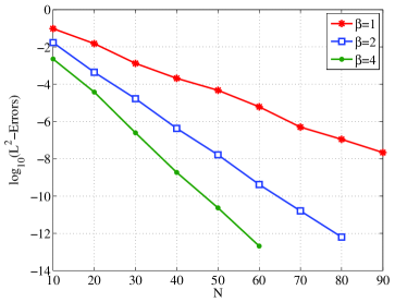
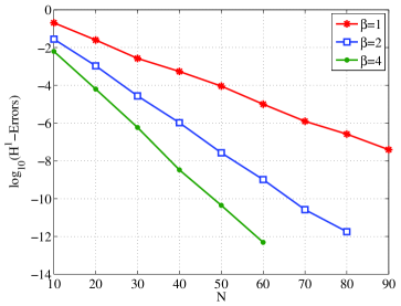
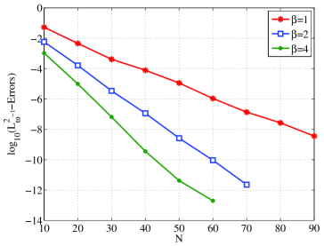
which is exponential decay with oscillation. In Figures 5.2, 5.2 and 5.4, we plot the of the discrete -, - and -errors vs. with various values of . Clearly, the approximate solutions converge at exponential rates. We also see that for fixed , the scheme with produces better numerical results than that with However, the choice of the optimal scaling factor for a given differential equation is still an open problem. Generally speaking, the choice of depends on the asymptotic behavior of solutions.
-
•
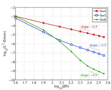
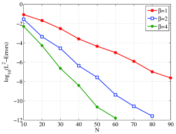
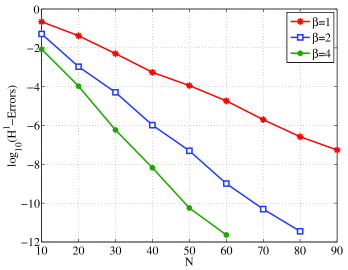
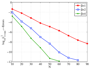
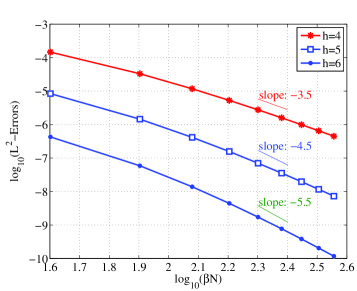
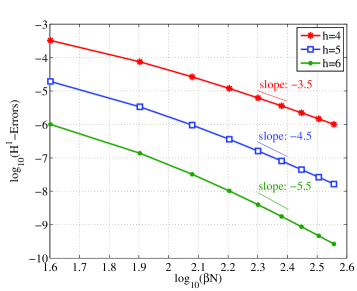
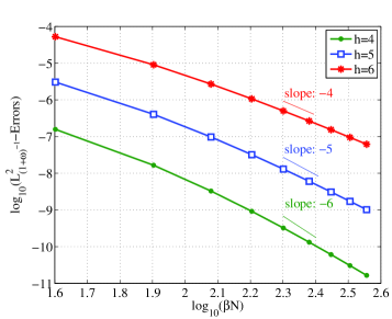
with which is algebraic decay. In Figures 5.4, 5.6 and 5.6, we plot the of the discrete -, - and -errors vs. with fixed and various values of . They show that the faster the exact solution decays, the smaller the numerical errors would be. Clearly,
According to Theorem 4.2, the expected - and -errors can be bounded by for any , and the expected -error can be bounded by for any . The observed convergence rates plotted in Figures 5.4, 5.6 and 5.6 agree well with the theoretical results.
-
•
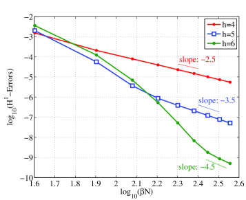
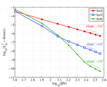
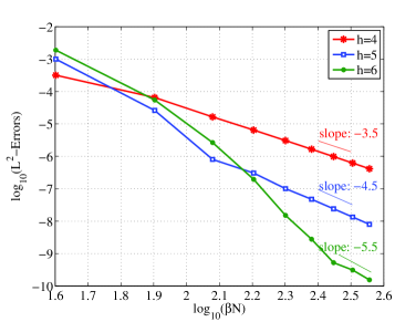
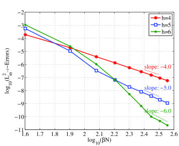
, which is algebraic decay with oscillation. In Figures 5.8, 5.8 and 5.10, we plot the of the discrete -, - and -errors vs. with fixed and various values of . Since
the expected -, - (resp. -) errors given by Theorem 4.2 can be bounded by (resp. ) for any . The observed convergence rates plotted in Figures 5.8, 5.8 and 5.10 also agree well with the theoretical results.
5.2. Robin boundary value problems
We take , and for the Robin boundary value problem (3.1) and consider two examples with different decay properties for the exact solutions.
- •
-
•
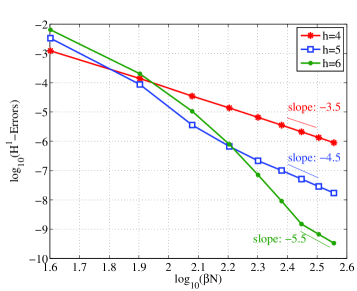
which is algebraic decay with oscillation. In Figures 5.14, 5.14 and 5.15, we plot the of the discrete -, - and -errors vs. with fixed and various values of . Since
the expected - and - (resp. -) errors given by Theorem 4.3 can be bounded by (resp. ) for any . Again, the observed convergence rates plotted in Figures 5.14, 5.14 and 5.15 agree well with the theoretical results.
5.3. On the condition numbers
To demonstrate the essential superiority of our diagonalized Laguerre spectral method to the classic Laguerre methods, we finally examine the issue on condition numbers for the resulting algebraic systems. The diagonalized Laguerre spectral method use the Sobolev-orthogonal Laguerre functions and as the basis functions for (3.8) and (3.3), respectively. All the condition numbers of the corresponding total stiff matrices are equal to . While in the classical Laguerre spectral method, the basis functions for (3.8) and (3.3) are chosen as and , respectively. The corresponding total stiff matrices have off-diagonal entries.
In Table 5.1 below, we list the condition numbers of the total stiff matrices of the classical Laguerre spectral method for (3.6) with versus various and . The condition numbers of the classical Laguerre spectral method for (3.1) with and are tabulated in Table 5.2. We note that the condition numbers of the resulting systems increase asymptotically as
| N | |||
|---|---|---|---|
| 10 | 1.5899E+03 | 5.1603E+02 | 2.8771E+02 |
| 30 | 2.3557E+04 | 6.8162E+03 | 3.5015E+03 |
| 50 | 7.5948E+04 | 2.1307E+04 | 1.0654E+04 |
| 70 | 1.6112E+05 | 4.4494E+04 | 2.1921E+04 |
| 90 | 2.8034E+05 | 7.6647E+04 | 3.7394E+04 |
| 110 | 4.3446E+05 | 1.1795E+05 | 5.7137E+04 |
| 130 | 6.2409E+05 | 1.6853E+05 | 8.1197E+04 |
| 150 | 8.4971E+05 | 2.2850E+05 | 1.0961E+05 |
| N | |||
|---|---|---|---|
| 10 | 5.8863E+01 | 2.1075E+02 | 4.4972E+02 |
| 30 | 4.1557E+02 | 1.6049E+03 | 3.5610E+03 |
| 50 | 1.0965E+03 | 4.2960E+03 | 9.5913E+03 |
| 70 | 2.1016E+03 | 8.2840E+03 | 1.8540E+04 |
| 90 | 3.4309E+03 | 1.3569E+04 | 3.0407E+04 |
| 110 | 5.0845E+03 | 2.0151E+04 | 4.5191E+04 |
| 130 | 7.0623E+03 | 2.8029E+04 | 6.2894E+04 |
| 150 | 9.3643E+03 | 3.7205E+04 | 8.3515E+04 |
References
- [1] J. Bergh and J. Lfstrm, Interpolation Spaces, An Introduction, Spring-Verlag, Berlin, 1976.
- [2] J. P. Boyd, Spectral methods using rational basis functions on an infinite interval, J. Comput. Phys., 69(1987), 112-142.
- [3] J. P. Boyd, Orthogonal rational functions on a semi-infinite interval, J. Comput. Phys., 70(1987), 63-88.
- [4] J. P. Boyd, Chebyshev and Fourier spectral methods, Second edition, Dover, New York, 2001.
- [5] C. Canuto, M. Y. Hussaini, A. Quarteroni and T. A. Zang, Spectral Methods: Fundamentals in single domains, Springer-Verlag, Berlin, 2006.
- [6] O. Coulaud, D. Funaro and O. Kavian, Laugerre spectral approximation of elliptic problems in exterior domains, Comp. Meth. in Appl. Mech. and Eng., 80(1990), 451-458.
- [7] C. I. Christov, A complete orthogonal system of functions in space, SIAM J. Appl. Math., 42(1982), 1337-1344.
- [8] L. Fernandez, F. Marcellan, T. Pérez, M. Piñar and Xu Yuan, Sobolev orthogonal polynomials on product domains. J. Comp. Anal. Appl., 284(2015), 202-215.
- [9] Guo Ben-yu, Jacobi approximations in certain Hilbert spaces and their applications to singular differential equations, J. Math. Anal. Appl., 243(2000), 373-408.
- [10] Guo Ben-yu and Shen Jie, Laguerre-Galerkin method for nonlinear partial differential equations on a semi-infinite interval, Numer. Math., 86(2000), 635-654.
- [11] Guo Ben-yu, Shen Jie and Wang Zhong-qing, A rational approximation and its applications to differential equations on the half line, J. Sci. Comput., 15(2000), 117-147.
- [12] Guo Ben-yu, Shen Jie and Wang Zhong-qing, Chebyshev rational spectral and pseudospectral methods on a semi-infinite interval, Internat. J. Numer. Methods Engrg., 53(2002), 65-84.
- [13] Guo Ben-yu, Shen Jie and Xu Cheng-long, Generalized Laguerre approximation and its applications to exterior problems, J. Comp. Math., 23(2005), 113-130.
- [14] Guo Ben-yu, Sun Tao and Zhang Chao, Jacobi and Laguerre quasi-orthogonal approximations and related interpolations, Math. Comp., 82(2013), 413-441.
- [15] Guo Ben-yu, Wang Li-lian and Wang Zhong-qing, Generalized Laguerre interpolation and pseudospectral method for unbounded domain, SIAM J. Numer. Anal., 43(2006), 2567-2589.
- [16] Guo Ben-yu and Zhang Xiao-yong, A new generalized Laguerre spectral approximation and its applications, J. Comp. Appl. Math., 181(2005), 342-363.
- [17] Guo Ben-yu and Zhang Xiao-yong, Spectral method for differential equations of degenerate type on unbounded domains by using generalized Laguerre functions, Appl. Numer. Math., 57(2007), 455-471.
- [18] V. Iranzo and A. Falquès, Some spectral approximations for differential equations in unbounded domains, Comput. Methods Appl. Mech. Engrg., 98(1992), 105-126.
- [19] Ma He-ping and Guo Ben-yu, Composite Legendre-Laguerre pseudospectral approximation in unbounded domains, IMA J. Numer. Anal., 21(2001), 587-602.
- [20] Y. Maday, B. Pernaud-Thomas and H.Vanderen, Reappraisal of Laguerre type spectral methods, Rech. Aérospat., 6(1985), 353-375.
- [21] F. Marcellán and Xu Yuan, On Sobolev orthogonal polynomials, Expo. Math., 33(2015), 308-352.
- [22] D. Nicholls and Jie Shen, A stable high-order method for two-dimensional bounded-obstacle scattering, SIAM J. Sci. Comput., 28(2006), 1398-1419.
- [23] Teresa E. Pérez and Miguel A. Piñar, On Sobolev orthogonality for the generalized Laguerre polynomials, J. Approx. Theory, 86(1996), 278-285.
- [24] Shen Jie, Stable and efficient spectral methods in unbounded domains using Laguerre functions, SIAM J. Numer. Anal., 38(2000), 1113-1133.
- [25] Shen Jie, Tang Tao and Wang Li-lian, Spectral Methods: Algorithms, Analysis and Applications, Springer Series in Computational Mathematics, Vol. 41, Springer, 2011.
- [26] Shen Jie and Wang Li-lian, Analysis of a spectral-Galerkin approximation to the Helmholtz equation in exterior domains, SIAM J. Numer. Anal., 45(2007), 1954-1978.
- [27] Shen Jie and Wang Li-lian, Some recent advances on spectral methods for unbounded domains, Commun. in Comp. Phys., 5(2009), 195-241.
- [28] Shen Jie and Wang Li-lian, Fourierization of the Legendre-Galerkin method and a new space-time spectral method, Applied Numerical Mathematics, 57(2007), 710-720.
- [29] G. Szegö, Orthogonal Polynomials (fourth edition), Vol. 23, AMS Coll. Publ., 1975.
- [30] Wang Zhong-qing, Guo Ben-yu and Wu Yan-na, Pseudospectral method using generalized Laguerre functions for singular problems on unbounded domains, Discrete Contin. Dyn. Syst. Ser. B, 11(2009), 1019-1038.
- [31] Wang Zhong-qing and Guo Ben-yu, Jacobi rational approximation and spectral method for differential equations of degenerate type, Math. Comp., 77(2008), 883-907.
- [32] Wang Zhong-qing and Xiang Xin-min, Generalized Laguerre approximations and spectral method for the Camassa-Holm equation, IMA J. Numer. Anal., 35(2015), 1456-1482.
- [33] Xu Cheng-long and Guo Ben-yu, Laguerre pseudospectral method for nonlinear partial differential equations, J. Comp. Math., 20(2002), 413-428.
- [34] Yi Yong-gang and Guo Ben-yu, Generalized Jacobi rational spectral method on the half line, Adv. Comput. Math., 37(2012), 1-37.
- [35] Zhuang Qing-qu, Shen Jie and Xu Chuan-ju, A coupled Legendre-Laguerre spectral-element method for the Navier-Stokes equations in unbounded domains, J. Sci. Comput., 42(2010), 1-22.