Local Scale-Invariance of the 2+1 dimensional Kardar–Parisi–Zhang model

Abstract

Local Scale-Invariance theory is tested by extensive dynamical simulations of the driven dimer lattice gas model, describing the surface growth of the 2+1 dimensional Kardar–Parisi–Zhang surfaces. Very precise measurements of the universal autoresponse function enabled us to perform nonlinear fitting with the scaling forms, suggested by local scale-invariance (LSI). While the simple LSI ansatz does not seem to work, forms based on logarithmic extension of LSI provide satisfactory description of the full (measured) time evolution of the autoresponse function.

Understanding universal scaling behavior of nonequilibrium dynamical systems is a challenging task [1]. Critical phenomena can emerge away from equilibrium, but due to the broken time reversal and translational symmetries, an extension of the Renormalization Group method (RG), as the best tool, is not straightforward [2]. The lack of translational symmetry manifests in aging phenomena observed in glasses, polymers, reaction-diffusion systems or cross-linked networks [3].

LSI theory is proposed [4] to generalize dynamical scaling to a larger set of local scale transformations, including $t\to t/(1+t\gamma)$, analogously as conformal invariance (CI) extends RG of equilibrium critical phenomena. As CI [5, 6] works well in case of equilibrium universality classes, LSI aims at the same for nonequilibrium dynamical ones [7]. LSI has been shown to reproduce the universal shapes of responses and correlators in a large variety of models, as reviewed in detail in [7]. The predictive power of generalized dynamical scaling alone was shown to be limited [8], and later the role of the generalized Galilei invariance was recognized. Analogously to the logarithmic CI generalization [9], Henkel suggested the logarithmic extension of LSI (LLSI) to make the theory applicable for more general cases [10].

While many systems are described by a single dynamical length scale $L(t)\sim t^{1/z}$, with the dynamical exponent $z$ [11, 12], aging ones are best characterized by two-time quantities, such as the dynamical correlation and response functions [13]. In the aging regime: $s\gg\tau_{\rm m}$ and $t-s\gg\tau_{\rm m}$, where $\tau_{\rm m}$ is a microscopic time scale, one expects the following law for the autoresponse function of the field $\phi$:

$$R(t,s)=\left.\frac{\delta\left\langle\phi(t)\right\rangle}{\delta j(s)}\right|_{j=0}=s^{-1-a}f_{R}\left(\frac{t}{s}\right)$$ (1)

where $s$ denotes the start and $t>s$ the observation time, $j$ is the external conjugate to $\phi$. This law contains the so-called aging exponent $a$, the universal scaling function, with the asymptotic behavior $f_{R}(t/s)\sim(t/s)^{-\lambda_{R}/z}$, and the autoresponse exponent $\lambda_{R}$.

LSI has been shown to describe aging properties of diffusive, solvable models with $z=2$, like Acetri [14, 15], Edwards–Wilkinson (EW) [16] interface growth and of mean-field like models, exhibiting long-range interactions [17, 7]. It also provided agreement with the numerics in case of reaction-diffusion models [18, 19, 20]. However, tests in the critical (1+1)-dimensional contact process showed systematic deviations in the $t/s\to 1$ limit [21, 10]. On a phenomenological level, these discrepancies could be resolved by the more recent extension to LLSI [10], which we shall recall below.

Numerical testing is easier in systems, which do not need to be tuned to criticality, but exhibit generic scale invariance, like interface models. For nonequilibrium surface growth dynamics the LLSI predictions have been found to be in agreement with the simulations of the $1+1$ dimensional Kardar–Parisi–Zhang (KPZ) model [22]. The purpose of the present study is to extend such investigation to $2+1$ dimensions in the presence of high precision simulation data available by simulations of dimer models describing KPZ surface growth [23, 24, 25].

The KPZ equation [26] describes the evolution of the height function $h(\mathbf{x},t)$ in the $d$ dimensional space relative to its mean position

$$\partial_{t}h(\mathbf{x},t)=\nu\nabla^{2}h(\mathbf{x},t)+\lambda(\nabla h(\mathbf{x},t))^{2}+\eta(\mathbf{x},t)\ ,$$ (2)

where $\lambda$ is the amplitude of the up-down anisotropy, $\nu$ is a smoothing surface tension coefficient and $\eta$ roughening the surface by a zero-mean-value Gaussian noise field exhibiting the variance $\langle\eta(\mathbf{x},t)\eta(\mathbf{x^{\prime}},t^{\prime})\rangle=2T\nu\delta^{d}(\mathbf{x-x^{\prime}})(t-t^{\prime})$. The letter $T$ is related to the noise amplitude (the temperature in the equilibrium system).

This equation was inspired in part by the stochastic Burgers equation [27] and can describe the dynamics of simple growth processes in the thermodynamic limit [28], randomly stirred fluids [29], directed polymers in random media [30], dissipative transport [31, 32], and the magnetic flux lines in superconductors [33].

The morphology of the surface is usually characterized by the roughness

$$W(L,t) =\sqrt{\left\langle h^{2}(\mathbf{x},t)\right\rangle_{\mathbf{x}}-\left\langle h(\mathbf{x},t)\right\rangle_{\mathbf{x}}^{2}}\quad,$$ (3)

where $$\left\langle\;\right\rangle_{\mathbf{x}}$$ denotes an average over all spatial coordinates. Simple growth processes are expected to be scale invariant and follow the Family-Vicsek scaling law [34]:

$$W(L,t) \sim L^{\alpha}f(t/L^{z})\quad,$$ (4)

with the universal scaling function $$f(u)$$,

$$f(u) \sim\begin{cases}u^{\beta}&\text{for }u\ll 1\\ \mathrm{const.}&\text{for }u\gg 1\ .\end{cases}$$ (5)

Here, $\alpha$ is the roughness exponent, describing the stationary state, where the correlation length exceeds the lateral system size $L$. The growth regime is governed by the growth exponent $\beta$. The ratio of these gives the dynamical exponent $z=\alpha/\beta$. KPZ is invariant to the Galilean symmetry [29], resulting in the exponent relation

$$z=2/\left(1+\beta\right)\quad.$$ (6)

Discrete models set up for KPZ have been studied a lot in the past decades [35, 36, 37]. A mapping between KPZ surface growth in two dimensions and driven lattice gases has been advanced in [23]. This is based on the so-called octahedron model, characterized by binary slope variables at the middle points of the up/down edges. Up slopes in the x or y directions are represented by $\sigma_{x/y}=1$, while down ones are encoded by $\sigma_{x/y}=0$. Thus deposition or removal of octahedra corresponds to a stochastic cellular automaton with the simple update rules

$$\left(\begin{array}[]{cc}0&1\\ 0&1\end{array}\right)\overset{p}{\underset{q}{\rightleftharpoons}}\left(\begin{array}[]{cc}1&0\\ 1&0\end{array}\right)$$ (7)

with probability $p$ ($q$) for attachment (detachment). By considering edge values to be lattice occupancy variables we can map the octahedron model onto self-reconstructing dimers following an oriented migration in the bisection of $x$ and $y$ directions (see Fig. in [23]). The surface height can be reconstructed for each lattice site from the slope variables by tracing a path from a reference point: $(1,1)$ with $h_{1,1}:=0$, leading to the expression

$$h_{i,j}=\sum_{l=1}^{i}[2\sigma_{x}(l,1)-1]+\sum_{k=1}^{j}[2\sigma_{y}(i,k)-1]\ .$$ (8)

We have confirmed that this mapping using the parameterization: $\lambda=2p/(p+q)-1$ reproduces the one-point functions of the continuum model [23]. The case $p\approx q$, leading to $\lambda\approx 0$, the EW model is recovered. Numerical results for the autocorrelation have also been found to be in agreement with those of other KPZ models [25, 38, 39]. The dimer lattice gas can be studied by very efficient bit coded simulation methods using graphic cards (GPU) as detailed in [40, 25].

We performed extensive simulations of the dimer model on lattices with lateral size of $L=2^{16}$ and periodic boundary conditions. The large systems serve to stay clear of finite size effects. The initial state corresponded to the flat surface and rule (7) was applied either by a random-sequential (RS) [25] or a sub-lattice parallel stochastic cellular automaton (SCA) site selection algorithm.

We calculated the autoresponse function as described in [25]. To introduce a perturbation, we used space-dependent attachment and detachment probabilities

$$p_{i}=\begin{cases}p_{0}+a_{i}\varepsilon/2&\text{if }p_{0}+a_{i}\varepsilon/2\in[0,1]\\ 1-\varepsilon/2+a_{i}\varepsilon/2&\text{otherwise}\end{cases}$$ (9)

and $q_{i}=p_{0}+q_{0}-p_{i}$, respectively. Here, $a_{i}=\pm 1$ and $\varepsilon=0.005$ is a small parameter. After the waiting time $s$ we used the same stochastic noise $\eta$ (random sequences), in two realizations. System A evolved, up to the waiting time $s$, with the site-dependent probabilities $p_{i}$ and $q_{i}$ and afterwards with the uniform ones $p_{0}$ and $q_{0}=0$. System B evolved always with spatially uniform attachment and detachment.

From these simulations, we determined the time-integrated response function

$$\chi(t,s)=\int_{0}^{s}\!\!{\rm d}u\>R(t,u)$$

$$= \frac{1}{L^{2}}\sum_{\vec{r}}^{L^{2}}\left\langle\frac{h_{\vec{r}}^{(A)}(t,s)-h_{\vec{r}}^{(B)}(t)}{\varepsilon\Delta}\right\rangle=s^{-a}f_{\chi}\left(\frac{t}{s}\right)\quad,$$

where $a$ is the aging exponent for the autoresponse. Measurements were performed at exponentially increasing times

$$t_{i+1}=(t_{i}+10)\cdot\mathrm{e}^{m},\quad\text{with}\quad m>0,\quad t_{0}=0\quad,$$

up to $t_{\mathrm{max}}=200\cdot s$. Throughout this paper time is measured in Monte-Carlo steps (MCS), defined as one sweep over all lattice sites.

The random-sequential GPU implementation from [25] has been modified using a novel combination of the dead border and double tiling domain-decomposition schemes, which we call DTrDB, in order to eliminate previously observed correlations. Details of this algorithm will be discussed elsewhere [41]. To speed up simulations further, we introduced a SCA algorithm on GPUs, which uses a checkerboard pattern for updates: A MCS is performed by updating all odd sites simultaneously with $p<1$ and all even sites afterwards [42]. The GPU implementations were tested by comparing different schemes. Direct comparison of the GPU results with sequential CPU simulations was impossible on the same level of accuracy, but consistency with former simulations [25] could be achieved.

Figure 1: Simulation results of the integrated height autoresponse, comparing variants obtained by RS and SCA simulations. (a): Aging collapse of the functions. (b): Corresponding effective exponents, extrapolating to asymptotic values. Slopes of DTrDB and SCA * are not shown, because the late-time regime was too noisy, due to small sample sizes. The black straight line corresponds to a linear fit to the SCA $s=30$ results. System and sample sizes are: $L_{\mathrm{\lx@glossaries@gls@link{acronym}{cpu}{\leavevmode CPU}*}}=2^{13}$, $n_{\mathrm{\lx@glossaries@gls@link{acronym}{cpu}{\leavevmode CPU}*}}=39083$ [25], all others use $L=2^{16}$, with $n_{\mathrm{\lx@glossaries@gls@link{acronym}{sca}{\leavevmode SCA}},s=30}=23849$, $n_{\mathrm{\lx@glossaries@gls@link{acronym}{sca}{\leavevmode SCA}},s=100}=12012$, $n_{\mathrm{\lx@glossaries@gls@link{acronym}{sca}{\leavevmode SCA}*},s=100}=1390$, $n_{\mathrm{DTrDB},s=30}=830$ and $n_{\mathrm{DTrDB},s=100}=700$.

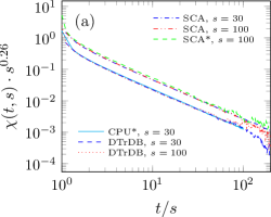
Results from various autoresponse calculations are summarized in Fig. 1(a). The forms of the autoresponse function agree very well across all types of simulations. The most notable difference is a constant factor ($\sim\num{2.08}$) in the response functions between the SCA and RS results, which is caused by model-dependent time-scales. Also note the small shift between SCA ($p=\num{.95},q=0$) and SCA * ($p=\num{.95},q=\num{.05}$) for $s=100$, caused by the different update probabilities.

The aging exponent is often determined by performing a manual collapse of the available datasets for different waiting times $s$. For RS simulations, the value $a_{\text{\lx@glossaries@gls@link{acronym}{rs}{\leavevmode RS}}}^{\text{coll.}}=\num{.30}(1)$ was determined in this way and published in [25]. For the SCA simulations presented in Fig. 1(a), the value $a_{\text{\lx@glossaries@gls@link{acronym}{sca}{\leavevmode SCA}}}^{\text{coll.}}=\num{.26}(1)$ shows the best collapse. However, this method requires visual inspection of plots to determine for which value of $a^{\text{coll.}}$ the data collapse works best, which is prone to bias and underestimation of the attached error margins.

Numerical computation of the aging exponent involves point-wise division of autocorrelation functions for different waiting times:

$$\frac{\chi(t,s_{1})}{\chi(t,s_{2})}=\frac{s_{1}^{a}f_{\chi}(t/s_{1})}{s_{2}^{a}f_{\chi}(t/s_{2})}\overset{(t/s_{1}=t/s_{2})}{=}\left(\frac{s_{1}}{s_{2}}\right)^{a}$$

Since the values $\left\langle\chi(t,s)\right\rangle$ are available only at discrete times an interpolation is required to compute these ratios at arbitrary $t/s$. The simplest option is a linear one, which can also be performed on a double-logarithmic scale, reducing systematic errors when the interpolation values follow a power law. In the implicit average over $t$ all points are weighted with their statistical signal-to-noise ratio, which overall increases the weight of early times, while in the visual method one is tempted to focus on late times. The present method yields $a_{\text{\lx@glossaries@gls@link{acronym}{sca}{\leavevmode SCA}}}=\num{.24}(2)$, for the SCA simulations with $q=0$, and $a_{\text{DTrDB}}=\num{.27}(2)$, for our new RS simulations with $p=1,q=0$. For comparison, we calculated $a_{\text{\lx@glossaries@gls@link{acronym}{rs}{\leavevmode RS}}}=\num{.25}(4)$ from the data published in [25], based on RS CPU and GPU simulations. The present data suggest no significant difference between the aging exponents of RS and SCA.

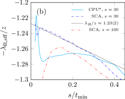
In order to determine the asymptotic scaling and corrections we determined (tail) effective exponents $\lambda_{R,\mathrm{eff}}(t_{\mathrm{min}})/z$, where each value is the exponent of a power-law fit to $\chi(t,s)$ in the interval $(t_{\mathrm{min}},t_{\mathrm{max}})$ using the form

$$g_{t_{\mathrm{min}}}(t)=c\cdot t^{-\lambda_{R,\mathrm{eff}}(t_{\mathrm{min}})/z}\ ,$$ (11)

with free parameters $c$ and $\lambda_{R,\mathrm{eff}}(t_{\mathrm{min}})/z$. The results are displayed in Fig. 1(b) for the three largest datasets, where $t_{\mathrm{min}}\lesssim t_{\mathrm{max}}/4$. This method suppresses short-wavelength noise but preserves scaling corrections of larger scales. Only our best dataset (SCA, $s=30$) allows a reliable extrapolation for ${\lambda_{R,\mathrm{eff}}(t_{\mathrm{min}}\to\infty,)/z}$. The effective exponent curve of the $s=100$ data breaks down at the end; still the trend observed at early times is in agreement with the extrapolations for $s=30$. We attribute this to larger oscillations, similarly as in the case of CPU RS updates, where, however, the asymptotic value still appears to agree.

Table 1 summarizes the estimates for the autoresponse exponent $\lambda_{R}$. Here we assume $z=1.611(2)$, that can be obtained by the scaling relation (6) and using our former, high precision value $\beta=0.2415(15)$ [24]. There is agreement between the results for the considered waiting times across RS and SCA dynamics.

Considering, that earlier results for the autocorrelation exponent marginally allow $\lambda_{C}=2$ [25], which is predicted by Krug’s conjecture $\lambda_{C}=d$ [43, 44], it is interesting to note, that $\lambda_{R}=2$ seems to be satisfied within error margin. The possible equality $\lambda_{C}=\lambda_{R}$ might point to the existence of a non-equilibrium fluctuation-dissipation relation in (2+1)-dimensional KPZ. The autocorrelation function is defined as

$$C(t,s)=\left\langle\phi(t)\phi(s)\right\rangle-\left\langle\phi(t)\right\rangle\left\langle\phi(s)\right\rangle\sim s^{-b}(t/s)^{-\lambda_{C}/z}\quad,$$

with the aging exponent $b=-2\beta$ and definitions analogous to those in Eq. (1). However, one must expect a different relation than in the (1+1)-dimensional case, because the implied relation for the aging exponents $1+a=b+2/z$ [22] does not hold.

Table 1: Estimates for the height autoresponse exponent $\lambda_{R}$, assuming $z=1.611(2)$. Sample and system sizes are listed below Fig. 1. Error-margins were estimated visually.

	CPU * [25]	SCA
	$p=\num{.98},q=\num{.02}$	$p=\num{.95},q=0$
$\lambda_{R}/z$	1.25(3)	1.23(2)
$\lambda_{R}$	2.01(5)	1.98(4)

The quality of the available data allows a precise calculation of effective exponents. Yet, the estimates for the asymptotic values carry larger uncertainties, due to the unknown corrections to scaling. Thus, a next step in the KPZ aging studies is an attempt to determine these corrections, assuming scaling forms for $\chi_{R}$. These forms are based on the LSI hypothesis. For the time-integrated autoresponse, Eq. (Local Scale-Invariance of the 2+1 dimensional Kardar–Parisi–Zhang model), LSI theory for KPZ predicts the scaling function

$$f_{\chi,\mathrm{LSI}}(t/s) =A_{0}(t/s)^{-\lambda_{R}/z}\left(1-s/t\right)^{-1-a^{\prime}}\quad,$$ (12)

where $A_{0}$ is a normalization factor and $a^{\prime}$ is expected to be another universal exponent, like the aging exponent $a$. A different form, adding logarithmic corrections was proposed recently in [10]:

$$f_{\chi,\mathrm{L^{2}LSI}} =(t/s)^{1-\lambda_{R}/z}\left[A_{0}\left(1-(1-s/t)^{-a^{\prime}}\right)\right.$$

$$+\left.(1-s/t)^{-a^{\prime}}\cdot\left(A_{1}\ln(1-s/t)+A_{2}\ln^{2}(1-s/t)\right)\right]\quad,$$ (13)

where the sum of logarithmic terms to second order results from the assumption, that the primary field $\phi$ of the system is replaced by a doublet and the scaling dimensions are represented by $2\times 2$ matrices. The solution in [10] uses a Schrödinger-invariant Lie algebra, which implies $z=2$, a dynamical exponent different from that of the KPZ universality class. However, the scaling form (1) is invariant of the value of $z$, because it depends on the ratio $\lambda_{R}/z$ only. It should be noted, that, this does not hold for the space-dependent part of the response function, which remains an open problem.

The scaling function (13) resembles a form, which contains the first two lowest order correction terms of a logarithmic series to (12). We shall test by fitting if, an assumed more generalized power series form

$$f_{\chi,\mathrm{L^{J}LSI}} =(t/s)^{1-\lambda_{R}/z}\left[A_{0}\left(1-(1-s/t)^{-a^{\prime}}\right)\right.$$

$$+\left.(1-s/t)^{-a^{\prime}}\cdot\sum\limits_{j>0}^{J}A_{j}\ln^{j}(1-s/t)\right]\quad,$$ (14)

which, given enough terms, might fit a broad range of data, really supports the expected L²LSI theory with the scaling (13). However, an LSI extension with triplets, or beyond, would also give physical meaning to some terms with $j\geq 3$. Thus these terms being relevant to describe the data would point to the necessity of higher orders in the extension of LSI.

Figure 2: Plots of Eq. (15) in case of SCA autoresponse calculations with $p=\num{.95}$ and $q=0$. Sample sizes are $n_{\mathrm{\lx@glossaries@gls@link{acronym}{sca}{\leavevmode SCA}},s=30}=23849$ for $s=30$ (a) and $n_{\mathrm{\lx@glossaries@gls@link{acronym}{sca}{\leavevmode SCA}},s=100}=12012$ for $s=100$ (b). Best fits are determined from the region $1\leq t/s\leq 10$.

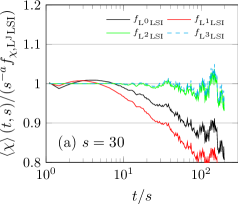
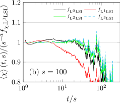
We have tested different ($J$) levels of the series (14) with our data, obtained from the most precise SCA simulations. Figure 2 shows plots of the ratio of data and best fit. This is a visual representation of how well forms for $J\in[0,3]$ describe the data:

$$\frac{\left\langle\chi\right\rangle(t/s)}{s^{-a}f_{\chi,\mathrm{L^{J}LSI}}(t/s)}\overset{!}{=}1\qquad\text{for }t/s>1\quad.$$ (15)

Table 2: Parameters for best fits of $f_{\chi,\mathrm{L^{J}LSI}}$ forms to KPZ autoresponse functions for $1\leq t/s\leq 200$. Values for $\lambda_{R}/z$ in parenthesis result from fits considering $q\leq t/s\leq 10$, as presented in figure 2. $a=\num{.24}$ for all fits. Error margins are not given, because the method employed for fitting does not provide meaningful estimates.

		$\lambda_{R}/z$	$a^{\prime}$	$A_{0}$	$A_{1}$	$A_{2}$	$A_{3}$
$s=30$	$f_{\mathrm{L^{0}LSI}}$	1.164 (1.167)	0.016	38.833
	$f_{\mathrm{L^{1}LSI}}$	1.164 (1.144)	0.023	35.085	0.187
	$f_{\mathrm{L^{2}LSI}}$	1.224 (1.219)	0.501	4.938	1.772	-0.431
	$f_{\mathrm{L^{3}LSI}}$	1.224 (1.224)	0.505	4.790	1.716	-0.422	-0.004
$s=100$	$f_{\mathrm{L^{0}LSI}}$	1.186 (1.191)	0.006	102.584
	$f_{\mathrm{L^{1}LSI}}$	1.165 (1.142)	0.100	14.444	0.844
	$f_{\mathrm{L^{2}LSI}}$	1.230 (1.224)	0.490	5.544	2.019	-0.472
	$f_{\mathrm{L^{3}LSI}}$	1.230 (1.233)	0.475	5.506	1.914	-0.437	-0.008

Non-linear fits for $J>0$ do not converge using the classical least-squares Levenberg–Marquardt algorithm [45, 46]. To obtain the parameters presented in table 2, the Nelder-Mead method [47] was employed, which does not provide statistical error estimates for the fit parameters. Fit results can be governed by any of a multitude of local minima, depending on the initial guesses and the choosen fit interval. Judging by the connected variation in parameter values, the accuracy of the tabulated parameters should be assumed to be no better than 20%, except for the values of $\lambda_{R}/z$ which vary by less than 5%.

It is apparent from figure 2 that the uncorrected LSI ansatz fails to describe the asymptotic behavior of $\chi$, giving $\lambda_{R}/z\approx\num{1.17}$. So does the logarithmic form with $J=1$. The form with $J=2$, which is predicted by the theory yields much better fits, with $\lambda_{R}/z\approx\num{1.22}$, agreeing with the asymptotic value obtained earlier $\lambda_{R}^{\mathrm{tail}}/z=\num{1.23}(2)$. The parameter fits presented in table 2 take into account the observed time interval $1\leq t/s\leq 200$. When the fit is limited to the interval $1\leq t/s\leq 10$, the results for $\lambda_{R}$ (values in parentheses) do not change significantly. This means, that the $f_{\chi,\mathrm{L^{2}LSI}}$ form describes the corrections, affecting the autoresponse function at early times, well enough to determine the correct asymptotic autoresponse exponent just using early-time data.

The form with $J=3$ shows marginally better agreement with the data in figure 2. In fits to the whole observed time interval, the amplitude $A_{3}$ of the added third-order term is severely suppressed (table 2). Adding another fit parameter, a slightly better fit would be expected. The small absolute value of $A_{3}$ in relation to $A_{2}$ suggests, that a third order correction does not carry physical meaning, supporting the L²LSI theory.

The values of the coefficients for $J=2$ and $3$ are similar at different waiting times. This satisfies our expectation, since aging is described by the $s^{-a}$ term in equation (Local Scale-Invariance of the 2+1 dimensional Kardar–Parisi–Zhang model) alone and the functional form of $f_{\chi}(t/s)$ should not depend on $s$ explicitly. The autoresponse functions we obtained by less precise simulations also agree with the L²LSI theory, but they exhibit too much noise to exclude a logarithmic series like (14).

In conclusion, we provide numerical evidence that the L²LSI theory describes well aging data of the autoresponse function for all measured times in case of the $2+1$ dimensional KPZ surface growth. We obtained precise estimates for the autoresponse exponent as well as for the aging exponents. In particular a $\lambda_{R}=2.00(6)$ estimate seems to emerge from our high precision parallel simulations. Our code can be extended to also calculate the space-dependent part of the KPZ response function. For the autocorrelation functions of the KPZ model $f_{C,\mathrm{L^{2}LSI}}$ a form is yet to be proposed. Our GPU simulations generate high precision correlation data for heights as well as density variables that remains to be tested later against different aging functions [41].

Acknowledgments:
We thank M. Henkel for helpful discussions and comments. Support from the Hungarian research fund OTKA (Grant No. K109577), the Initiative and Networking Fund of the Helmholtz Association via the W2/W3 Program (W2/W3-026) and the International Helmholtz Research School NanoNet (VH-KO-606) is acknowledged. We gratefully acknowledge computational resources provided by the HZDR computing center, NIIF Hungary and the Center for Information Services and High Performance Computing (ZIH) at TU Dresden.

References

- [1] Ódor G 2008 Universality in Nonequilibrium Lattice Systems (World Scientific)
- [2] Täuber U C 2014 Critical Dynamics (Cambridge University Press) ISBN 9781139046213 cambridge Books Online URL http://dx.doi.org/10.1017/CBO9781139046213
- [3] Struik L C E 1978 Physical Aging in Amorphous Polymers and Other Materials (Elsevier)
- [4] Henkel M 1994 J. Stat. Phys. 75 1023–1061 ISSN 1572-9613 URL http://dx.doi.org/10.1007/BF02186756
- [5] Cardy J L 1996 Scaling and Renormalization in Statistical Mechanics (Cambridge University Press)
- [6] Henkel M 1999 Conformal Invariance and Critical Phenomena (Springer)
- [7] Henkel M and Pleimling M 2010 Non-Equilibrium Phase Transitions: Volume 2: Ageing and Dynamical Scaling Far from Equilibrium Theoretical and Mathematical Physics (Springer Netherlands) ISBN 9789048128686 URL https://books.google.de/books?id=DN2gjwEACAAJ
- [8] Hinrichsen H 2008 J. Stat. Mech. 2008 P07026 URL http://stacks.iop.org/1742-5468/2008/i=07/a=P07026
- [9] Gurarie V 1993 Nucl. Phys. B 410 535–549 ISSN 0550-3213 URL http://www.sciencedirect.com/science/article/pii/055032139390528W
- [10] Henkel M 2013 Nucl. Phys. B 869 282–302 ISSN 0550-3213 URL http://www.sciencedirect.com/science/article/pii/S0550321312006682
- [11] Hohenberg P C and Halperin B I 1977 Rev. Mod. Phys. 49(3) 435–479 URL http://link.aps.org/doi/10.1103/RevModPhys.49.435
- [12] Bray A 1994 Adv. Phys. 43 357–459 URL http://dx.doi.org/10.1080/00018739400101505
- [13] Cugliandolo L F 2003 (Les Houches - Ecole d’Ete de Physique Theorique vol 77) (Springer) ISBN 978-3-540-40141-4
- [14] Henkel M and Durang X 2015 J. Stat. Mech. 2015 P05022 URL http://stacks.iop.org/1742-5468/2015/i=5/a=P05022
- [15] Henkel M 2015 Symmetry 7 2108 ISSN 2073-8994 URL http://www.mdpi.com/2073-8994/7/4/2108
- [16] Edwards S F and Wilkinson D R 1982 Proc. R. Soc. London, Ser. A 381 17–31 ISSN 0080-4630
- [17] Henkel M 2017 Symmetry 9 2 ISSN 2073-8994 URL http://www.mdpi.com/2073-8994/9/1/2
- [18] Enss T, Henkel M, Picone A and Schollwöck U 2004 J. Phys. A 37 10479 URL http://stacks.iop.org/0305-4470/37/i=44/a=002
- [19] Ódor G 2006 J. Stat. Mech. 2006 L11002 URL http://stacks.iop.org/1742-5468/2006/i=11/a=L11002
- [20] Henkel M 2007 J. Phys. Condens. Matter 19 065101 URL http://stacks.iop.org/0953-8984/19/i=6/a=065101
- [21] Hinrichsen H 2006 J. Stat. Mech. 2006 L06001 URL http://stacks.iop.org/1742-5468/2006/i=06/a=L06001
- [22] Henkel M, Noh J D and Pleimling M 2012 Phys. Rev. E 85(3) 030102 URL http://link.aps.org/doi/10.1103/PhysRevE.85.030102
- [23] Ódor G, Liedke B and Heinig K H 2009 Phys. Rev. E 79 021125
- [24] Kelling J and Ódor G 2011 Phys. Rev. E 84(6) 061150 URL http://link.aps.org/doi/10.1103/PhysRevE.84.061150
- [25] Ódor G, Kelling J and Gemming S 2014 Phys. Rev. E 89(3) 032146 URL http://link.aps.org/doi/10.1103/PhysRevE.89.032146
- [26] Kardar M, Parisi G and Zhang Y C 1986 Phys. Rev. Lett. 56(9) 889–892 URL http://link.aps.org/doi/10.1103/PhysRevLett.56.889
- [27] Burgers J M 1974 The nonlinear diffusion equation : asymptotic solutions and statistical problems (Dordrecht-Holland ; Boston : D. Reidel Pub. Co) ISBN 9027704945 first published in 1973 under title: Statistical problems connected with asymptotic solutions of the one-dimensional nonlinear diffusion equation
- [28] Halpin-Healy T 1990 Phys. Rev. A 42(2) 711–722 URL http://link.aps.org/doi/10.1103/PhysRevA.42.711
- [29] Forster D, Nelson D R and Stephen M J 1977 Phys. Rev. A 16(2) 732–749 URL http://link.aps.org/doi/10.1103/PhysRevA.16.732
- [30] Kardar M 1985 Phys. Rev. Lett. 55(26) 2923–2923 URL http://link.aps.org/doi/10.1103/PhysRevLett.55.2923
- [31] van Beijeren H, Kutner R and Spohn H 1985 Phys. Rev. Lett. 54(18) 2026–2029 URL http://link.aps.org/doi/10.1103/PhysRevLett.54.2026
- [32] Janssen H and Schmittmann B 1986 Z. Phys. B 63 517–520 ISSN 0722-3277 URL http://dx.doi.org/10.1007/BF01726201
- [33] Hwa T 1992 Phys. Rev. Lett. 69(10) 1552–1555 URL http://link.aps.org/doi/10.1103/PhysRevLett.69.1552
- [34] Family F and Vicsek T 1985 J. Phys. A 18 L75 URL http://stacks.iop.org/0305-4470/18/i=2/a=005
- [35] Meakin P, Ramanlal P, Sander L M and Ball R C 1986 Phys. Rev. A 34(6) 5091–5103 URL http://link.aps.org/doi/10.1103/PhysRevA.34.5091
- [36] Barabási A and Stanley H 1995 Fractal Concepts in Surface Growth (Cambridge University Press) ISBN 9780521483186 URL https://books.google.de/books?id=W4SqcNr8PLYC
- [37] Krug J 1997 Adv. Phys. 46 139–282 URL http://dx.doi.org/10.1080/00018739700101498
- [38] Halpin-Healy T and Palasantzas G 2014 EPL 105 50001 URL http://stacks.iop.org/0295-5075/105/i=5/a=50001
- [39] Carrasco I S S, Takeuchi K A, Ferreira S C and Oliveira T J 2014 New J. Phys. 16 123057 URL http://stacks.iop.org/1367-2630/16/i=12/a=123057
- [40] Kelling J, Ódor G, Nagy M F, Schulz H and Heinig K 2012 Eur. Phys. J.: Spec. Top. 210(1) 175–187 ISSN 1951-6355 10.1140/epjst/e2012-01645-8 URL http://dx.doi.org/10.1140/epjst/e2012-01645-8
- [41] Kelling J, Ódor G and Gemming S 2017 To be published
- [42] Kelling J, Ódor G and Gemming S 2016 Bit-vectorized GPU implementation of a stochastic cellular automaton model for surface growth 2016 IEEE 20th Jubilee International Conference on Intelligent Engineering Systems (INES) pp 233–237
- [43] Kallabis H and Krug J 1999 EPL 45 20 URL http://stacks.iop.org/0295-5075/45/i=1/a=020
- [44] Krech M 1997 Phys. Rev. E 55(1) 668–679 URL http://link.aps.org/doi/10.1103/PhysRevE.55.668
- [45] Levenberg K 1944 Q. J. Appl. Math. II 164–168
- [46] Marquardt D W 1963 J. Soc. Ind. Appl. Math. 11 431–441 (Preprint http://dx.doi.org/10.1137/0111030) URL http://dx.doi.org/10.1137/0111030
- [47] Nelder J A and Mead R 1965 Comput. J. 7 308–313 (Preprint http://comjnl.oxfordjournals.org/content/7/4/308.full.pdf+html) URL http://comjnl.oxfordjournals.org/content/7/4/308.abstract