Cycles and Clustering in Multiplex Networks

Abstract

In multiplex networks, cycles cannot be characterized only by their length, as edges may occur in different layers in different combinations. We define a classification of cycles by the number of edges in each layer and the number of switches between layers. We calculate the expected number of cycles of each type in the configuration model of a large sparse multiplex network. Our method accounts for the full degree distribution including correlations between degrees in different layers. In particular, we obtain the numbers of cycles of length $3$ of all possible types. Using these, we give a complete set of clustering coefficients and their expected values. We show that correlations between the degrees of a vertex in different layers strongly affect the number of cycles of a given type, and the number of switches between layers. Both increase with assortative correlations and are strongly decreased by disassortative correlations. The effect of correlations on clustering coefficients is equally pronounced.

I Introduction

The realization that many complex systems cannot be understood by representing them as a single network, has led to an explosion of interest in multilayer and multiplex (multiple types of edges) networks. Applications range from infrastructure Rinaldi et al. (2001), financial Huang et al. (2013), transport De Domenico et al. (2014) and ecological Pocock et al. (2012).

To properly study multilayer systems, it is essential to understand the fundamental properties of such structures. Many concepts from single layer networks have already been generalized to multiple layers, from the degree distribution, to connectivity, adjacency and Laplacian matrices, centrality measures and so on Boccaletti et al. (2014); Kivela et al. (2014); De Domenico et al. (2016). In many cases, the generalization of concepts from single networks—for example, the meaning of “giant connected component” Baxter et al. (2012, 2016)—is not straightforward, and introduces a new dimension to the problem.

In this Paper, we give an analytical description of the statistics of cycles in multiplex networks. In particular, we consider multiplex networks characterized by a given multi-degree distribution (configuration model). As this model is the starting point of any network analysis of a real-world system, it is easy to see how important it is to analytically characterize a structural property like the statistics of cycles. In a multilayer network, the possibility to switch between layers greatly increases the number of cycle types with respect to the single layer case. Cycles are then no longer defined simply by their length. We must take into account the proportion of the cycle in each layer, as well as the number of switches between layers. In particular, this leads to a set of different clustering coefficients generated by different cycles of length $3$.

Even when two cycles contain the same number of edges of each color, they can differ in the way colored edges are arranged within the cycle. We introduce a matrix $\mathbf{s}$ characterizing the number of edges of each color, and the number of switches between layers of a cycle. We give formulæ for calculating the mean number of cycles corresponding to a given $\mathbf{s}$ in a random graph with a given size and degree distribution. As examples, we calculate the distribution of edge colors and switches in cycles of a given length, show the effects of degree correlations between layers, and examine the special case of cycles of length $3$, which allows the calculation of the generalized clustering coefficients in multiplex networks.

The statistics of cycles is relevant both from a theoretical and an applicative point of view. From a theoretical perspective, it allows one to understand whether the distribution of cycles observed in a real world network is significantly different from that in a random graph with similar statistics Cozzo et al. (2015). Even in the single layer case, the high concentration of finite cycles in real-world networks has been a formidable barrier to analytic treatment, as mathematical models of large networks are typically based on the local tree-like assumption, i.e. the vanishing of density of finite cycles as the size of the network diverges Newman (2003); Bianconi and Capocci (2003); Bollobás and Riordan (2003). On the other hand, some analytic theories have been quite successful even in real-world networks Melnik et al. (2011), suggesting that the role played by the detailed architecture of topological correlations and cycles is not easily characterized. In multiplex networks, further types of correlations arise naturally, with implications for the structural properties of the multiplex Kim and Goh (2013); Hackett et al. (2016). It is therefore necessary to turn now to multiplex cycles and investigate the statistics of each category based on edge color and layer switches, and the effects of correlations on them. The properties of cycles is also an important topic of graph theory Bollobás (2001); Harary and Manvel (1971). A relatively smaller volume of work has been devoted to cycles on colored edge graphs, mainly involving only theorems of existence Abouelaoualim et al. (2010).

The statistics of cycles in multiplex networks is also relevant for a number of applications. In information technology, the presence of multiple paths of heterogeneous colors is a structural property that improves the robustness of a network Wang and Desmedt (2011) and the security of a wireless sensor network from a malicious attack Jain (2004). Multiplex cycles are also relevant when examining commuter behavior on multiple transport networks, as they provide alternative routes De Domenico et al. (2014). In such applications, switching between layers may have a time or monetary cost, a consideration which is absent in single layer networks. The statistics of switches is therefore an essential part of any analysis of cycles in multiplex networks.

This paper is organized as follows. In Section II, we describe a classification of cycles in multiplex networks and explain our formula to calculate the number of cycles within a given class. In Section III, we use our formula to calculate multiplex clustering coefficients. Finally, in Section IV we state our conclusions.

II Statistics of cycles

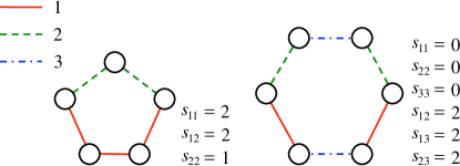
Figure 1: Notation of multiplex cycles.

We characterize a given cycle in a multiplex network, by the matrix $\mathbf{s}=\{s_{ab}\}_{a,b=1,\dots,M}$, where each element $s_{ab}$ defines the number of nodes in the cycle which connect an edge of type $a$ with an edge of type $b$. When $a=b$, this counts the number of nodes where the cycle remains in the same layer. When $a\neq b$, $s_{ab}$ counts the number of switches between layer $a$ and layer $b$. In this Paper, we identify and study the classes of equivalence of cycles with the same $\mathbf{s}$. In addition, here we only consider cycles without an orientation, therefore the order of the switches is not important, i.e. $s_{ba}=s_{ab}$. Examples of cycles with a given $\mathbf{s}$ are shown in Fig. 1. As a consequence of this definition, the total number of edges in layer $a$ is then $n_{a}=s_{aa}+\frac{1}{2}\sum_{b\neq a}s_{ab}$. Clearly, the number of switches must be such that $n_{a}$ is an integer for all $a$. The total length of a cycle $L$ is the sum of all entries of $\mathbf{s}$.

We consider a generalization of the configuration model to multiplex networks, i.e. large sparse random multiplex networks with $N$ nodes in $M$ layers, defined by the joint multidegree distribution $P(q_{1},q_{2},...,q_{M})$. This ensemble includes all possible configurations with multidegree sequence sampled from this distribution with equal statistical weight Bender and Canfield (1978); Bollobás (1980).

To calculate the mean number of cycles $\mathcal{N}(\mathbf{s})$ with a given $\mathbf{s}$ in a random graph, we first count the number of ways we can select, from the given multidegree distribution, the nodes that have the connectivity required for each $s_{ab}$; then, we count the number of ways we can connect these nodes to form a cycle. This method is similar to that used in, for example, Ref. Bianconi and Marsili (2005) but we extend it to account for edges of different colors and switches between layers. The results can be written as the product of several factors:

$$\mathcal{N}(\mathbf{s})=G(\mathbf{s})W(N,\mathbf{s})R[N,\mathbf{s},P(\mathbf{q})]\,,$$ (1)

where $R(N,\mathbf{s},P(\mathbf{q}))$ counts the number of ways one can select pairs of edges connected to $L$ nodes, in the correct numbers to match the elements of matrix $\mathbf{s}$, $W(N,\mathbf{s})$ counts the number of graphs in the ensemble containing the cycle, and $G(\mathbf{s})$ counts the number of ways of arranging the selected nodes to form a cycle. In principle one can complete this calculation for an arbitrary cycle in a multiplex with an arbitrary number of layers. However, the calculation of $G(\mathbf{s})$ becomes somewhat complicated for more than two layers, for anything but the shortest cycles.

Let us focus, now, on a two layer random multiplex (duplex), defined by the joint degree distribution $P(q_{1},q_{2})$. In the case of two layers, $\mathbf{s}$ has three entries: $s_{11}$, $s_{22}$, and $s_{12}$. For a given $L$, $s_{11}$ and $s_{22}$ can take any value from $0$ to $L$, while the number of switches $s_{12}\equiv 2p$, for integer $p$, to ensure that the number of edges of each color is integral, while all three must satisfy $s_{11}+s_{22}+s_{12}=L$. The formula (1) can be calculated explicitly in the asymptotic case characterized by $L\ll N$.

Without switches, $G(\mathbf{s})$ is simply the number of possible orderings of the $L$ nodes, dividing by $2L$ as each direction and starting point in the ordering is equivalent:

$$G(L,0,0)=\frac{L!}{2L}$$ (2)

and similarly for $G(0,L,0)$. When $s_{12}>0$, $G(\mathbf{s})$ is given by the number of ways of ordering the switches $(s_{12}-1)!$ multiplied by the number of ways $D(s_{11},p)D(s_{22},p)$ of placing the non-switching nodes in the spaces between the switches, where

$$D(s,p) = \sum_{n_{1}=0}^{l}{s\choose n_{1}}n_{1}!\sum_{n_{2}=0}^{s-n_{1}}{s-n_{1}\choose n_{2}}n_{2}\dots$$ (3)

$$\dots\sum_{n_{p-1}=0}^{s-\sum_{j=1}^{p-2}n_{j}}{s-\sum_{j=1}^{p-2}n_{j}\choose n_{p-1}}n_{p-1}!\left[s-\sum_{j=1}^{p-1}n_{j}\right]$$

$$= \frac{(s+p-1)!}{(p-1)!}$$

Thus

$$G(s_{11},s_{22},s_{12})=\left\{\begin{array}[]{lcrcl}(s_{12}-1)!D(s_{11},p)D(s_{22},p)&&s_{12}>0\\ \frac{(s_{11}+s_{22})!}{2(s_{11}+s_{22})}&&s_{12}=0\\ \end{array}\right..$$ (4)

The number of ways to form layer $1$ is the number of ways to connect $c_{1}N$ stubs in pairs: $(c_{1}N-1)(c_{1}N-3)...3\cdot 1=(c_{1}N-1)!!$, while the number of ways to connect the edges not forming part of the loop is $(c_{1}N-2s_{11}-s_{12}-1)!!$. Hence the fraction of layer $1$ configurations containing the loop is the ratio of these two numbers. Repeating for layer $2$, we find that $W(N,\mathbf{s})$ can be simply written

$$W(N,\mathbf{s})=\frac{(c_{1}N\!-\!2s_{11}\!-\!s_{12}\!-\!1)!!(c_{2}N\!-\!2s_{22}\!-\!s_{12}\!-\!1)!!}{(c_{1}N-1)!!(c_{2}N-1)!!}.$$ (5)

II.1 Formulæ for short cycles

When $L\ll N$, the factor $W(N,\mathbf{s})$ can be approximated as

$$W(N,\mathbf{s})=\frac{1}{N^{L}\langle q_{1}\rangle^{s_{11}+p}\langle q_{2}\rangle^{s_{22}+p}}.$$ (6)

Furthermore, we can treat the selection of nodes as being done with replacement, meaning that $R(N,\mathbf{s},P(\mathbf{q}))$ can be simply written as a product of terms for each node in the cycle:

$$R(N,\mathbf{s},P(\mathbf{q}))=\frac{N^{L}\langle q_{1}(q_{1}-1)\rangle^{s_{11}}\langle q_{2}(q_{2}-1)\rangle^{s_{22}}\langle q_{1}q_{2}\rangle^{s_{12}}}{s_{11}!s_{22}!s_{12}!}$$ (7)

where $\langle...\rangle$ indicates averages with respect to the degree distribution (ensemble averages).

When Eq. (7) is combined with $G(\mathbf{s})$ and $W(N,\mathbf{s})$ as given by Eqs. (4) and (6) we find that, when none of $s_{11},s_{22},s_{12}$ is zero,

$$\mathcal{N}(\mathbf{s}) =\binom{s_{11}+p-1}{s_{11}}\binom{s_{22}+p-1}{s_{22}}\frac{1}{2p}\left[\frac{\langle q_{1}(q_{1}-1)\rangle}{\langle q_{1}\rangle}\right]^{s_{11}}$$

$$\times \left[\frac{\langle q_{2}(q_{2}-1)\rangle}{\langle q_{2}\rangle}\right]^{s_{22}}\left[\frac{\langle q_{1}q_{2}\rangle}{\sqrt{\langle q_{1}\rangle\langle q_{2}\rangle}}\right]^{2p}\,,$$ (8)

In the case $s_{12}=0$, the cycle consists of only one color, so $\mathcal{N}(\mathbf{s})=0$ unless either $s_{22}=0$ or $s_{11}=0$, in which case

$$\mathcal{N}(L,0,0)=\frac{1}{2L}\left[\frac{\langle q_{1}(q_{1}-1)\rangle}{\langle q_{1}\rangle}\right]^{L}.$$ (9)

This coincides with the single layer result found in, for example, Ref. Bianconi and Marsili (2005). Similarly, the formula for $\mathcal{N}(0,L,0)$ is found simply by exchanging the subscripts.

On the other hand, when $s_{11}=0$, it is still possible to have $s_{12}>0$, when each segment in layer $1$ consists of only a single edge (i.e. each switch between layers is immediately followed by another switch). Then

$$\mathcal{N}(0,s_{22},2p)=\\ \binom{s_{22}+p-1}{s_{22}}\frac{1}{2p}\left[\frac{\langle q_{2}(q_{2}-1)\rangle}{\langle q_{2}\rangle}\right]^{s_{22}}\left[\frac{\langle q_{1}q_{2}\rangle}{\sqrt{\langle q_{1}\rangle\langle q_{2}\rangle}}\right]^{2p}\,,$$ (10)

and similarly for the case $s_{22}=0$ but $s_{12}>0$ and $s_{11}>0$, by exchanging the subscripts $1$ and $2$. If we project the two layers onto a single network, we recover the existing result for a single colored network, which has the same form as Eq. (9).

These results are valid for $L\ll N$, such as in the limit $N\to\infty$. The expected number of cycles in other cases, for longer cycles (when terms of $\mathcal{O}(1/N)$ can’t be neglected) can be found by a more precise derivation, which we outline in the Appendix.

II.2 Representative examples

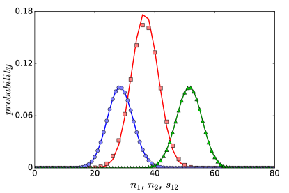
Figure 2: Distribution of number of edges of type $1$ (circles, blue online) and $2$ (triangles, green online) and number of switches $s_{12}$ (squares, red online) in cycles of length $L=80$ in two uncorrelated layers with Poisson degree distributions having mean degrees $\langle q_{1}\rangle=25$ and $\langle q_{2}\rangle=45$. Symbols are from summation of Eq. (II.1), solid lines are binomial distributions for $L$ trials with probabilities $\langle q_{1}\rangle/(\langle q_{1}\rangle+\langle q_{2}\rangle)$, $\langle q_{2}\rangle/(\langle q_{1}\rangle+\langle q_{2}\rangle)$, and $\langle q_{1}\rangle\langle q_{2}\rangle/(\langle q_{1}\rangle+\langle q_{2}\rangle)^{2}$ respectively.

The number of cycles having exactly $n_{1}=s_{11}+\frac{1}{2}s_{12}$ edges of type $1$ for a fixed $L$ can be found by summing Eq. (II.1) over each $s_{ab}$. In the absence of inter-layer degree correlations, the resulting distributions for $n_{1}$ match the Binomial distribution found by selecting $L$ edges at random from the network, as shown in Fig. 2. The mean number of type $1$ edges is $p_{1}=\langle q_{1}\rangle/(\langle q_{1}\rangle+\langle q_{2}\rangle)$, and similarly for $n_{2}$. In addition, the number of switches $s_{12}$, which must always be even, can be found by summing over $s_{11}$ and $s_{22}$. The mean number of switches $\langle s_{12}\rangle$ is well predicted by $2L\langle q_{1}\rangle\langle q_{2}\rangle/(\langle q_{1}\rangle+\langle q_{2}\rangle)^{2}$, which is the expected number of mismatches when pairing $L$ randomly chosen edges, and the distribution is also well matched by a binomial distribution.

The number of cycles for a given matrix $\mathbf{s}$ in Eq. (II.1) depends only on the moments of the joint degree distribution. This means that networks may have quite different degree distributions, and hence different structures, but if the relevant moments are the same, so will be the average number of cycles of each kind.

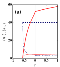
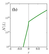
Figure 3: (a) Mean for $n_{1}$ (blue, dashed) and $s_{12}$ (red, heavy solid) and corresponding standard deviations (blue dash-dot, red light, respectively) as a function of Pearson correlation coefficient $r$ for the degrees of a vertex in different layers. Assortative correlations ($r<0$) are created using a joint degree distribution of the form $P(q_{1},q_{2})=\rho\frac{1}{2}[(P(q_{1})+P(q_{2})]\delta_{q_{1},q_{2}}+(1-\rho)P(q_{1})P(q_{2})$. disassortative correlations ($r<0$) are of the form $P(q_{1},q_{2})=\rho[(P(q_{1})\delta_{q_{2},0}+P(q_{2})\delta_{q_{1},0}]+(1-\rho)P(q_{1})P(q_{2})$, where $P(q)\propto q^{-\gamma}$, with $\gamma=3.7$, is a power-law distribution, and $L=80$. Maximum disassortative correlation occurs when the two layers no longer overlap, at which point $n_{1}=0$. The corresponding value of $r$ depends on $\gamma$. Figures are qualitatively similar for any value of $\gamma>3$. (b) Total number of cycles as a function of $r$.

In simplex networks, it has been shown that degree-degree correlations for neighboring vertices affect quite deeply the number of cycles Bianconi and Marsili (2006). In multiplex networks, it is natural to ask about the effect of degree correlations across layers. Indeed, we can see from the last term in Eq. (II.1) that interlayer degree correlations affect the number of cycles having a given number of switches between layers. For a given $L$, assortative interlayer degree correlations will tend to increase the number of switches, as high degree nodes in one layer, which are more frequently visited, will also have more available edges in the other layers. Conversely, disassortative correlations will tend to decrease the number of switches. The mean number of edges of type $1$ remains constant, although the distribution changes. These effects can be seen in Fig. 3, in which we plot the mean and standard deviation of $n_{1}$ and $s_{12}$ as a function of the Pearson correlation coefficient $r$ for the degrees of a vertex in different layers Newman (2003). We see that in the extreme case of disassortative correlations, there are no switches and the entire cycle is of one color, as the standard deviation of $n_{1}$ reaches the maximum value of $L/2$. An even more dramatic change is seen in the total number of cycles of a given length. The right panel in Fig. 3 shows the total number of cycles of length $L$ as a function of $r$. Disassortative correlations greatly restrict the possible number cycles that can be formed, while assortative correlations greatly increase it. Note that the apparently sharp inflections at $r=0$ result simply from the use of different functional forms for assortative and disassortative correlations.

III Clustering

The clustering coefficient of a network is related to the number of triangles, that is, cycles of length three. In such short cycles, the computation of factor $G(\mathbf{s})$ is straightforward, thus we can calculate the number of cycles of length $3$ for any number of layers. Such a cycle may be entirely within one layer: $\mathcal{N}_{m}^{(1)}=z_{m}^{3}/6c_{m}^{3}$; have two edges in one layer ($m$) and one edge in a second layer ($n$): $\mathcal{N}_{m,n}^{(2)}=z_{m}\langle q_{m}q_{n}\rangle^{2}/2c_{m}^{2}c_{n}$; or have one edge each in three different layers: $\mathcal{N}_{m,n,r}^{(3)}=\langle q_{m}q_{n}\rangle\langle q_{m}q_{r}\rangle\langle q_{n}q_{r}\rangle/c_{m}c_{n}c_{r}$ , where $z_{m}\equiv\langle q_{m}(q_{m}-1)\rangle$ and $c_{m}=\langle q_{m}\rangle$. We can then define a global clustering coefficient by

$$C =\frac{3\sum_{\mathbf{s}:L=3}\mathcal{N}(\mathbf{s})}{\mathcal{V}(N)}$$

$$=\frac{3{\displaystyle\sum_{m}}\mathcal{N}_{m}^{(1)}+3{\displaystyle\sum_{m,n\neq m}}\mathcal{N}_{m,n}^{(2)}+3{\displaystyle\sum_{\begin{subarray}{c}m,n\neq m\\ r\neq m,n\end{subarray}}}\mathcal{N}_{n,m,r}^{(3)}}{N\left[\sum_{m}z_{m}+2\sum_{m,n\neq m}\langle q_{m}q_{n}\rangle\right]}\,,$$ (11)

where $\mathcal{V}(N)$ is the number of adjacent edge-pairs in the graph, and the summation is over all cycle matrices $\mathbf{s}$ having length $L=3$.

One may also define partial clustering coefficients for triangles entirely within a given layer, two given layers, or three given layers ($C_{m,n,r}^{(3)}$) respectively:

$$C_{m}^{(1)} =\frac{3\mathcal{N}_{m}^{(1)}}{\frac{1}{2}Nz_{m}}=\frac{z_{m}^{2}}{Nc_{m}^{3}},$$ (12)

$$C_{m,n}^{(2)} =\frac{3\mathcal{N}_{m,n}^{(2)}}{\frac{1}{2}N\left[z_{m}+2\langle q_{m}q_{n}\rangle\right]}=\frac{3z_{m}\langle q_{m}q_{n}\rangle^{2}}{N\left[z_{m}+2\langle q_{m}q_{n}\rangle\right]c_{m}^{2}c_{n}},$$ (13)

$$C_{m,n,r}^{(3)} =\frac{3\mathcal{N}_{m,n,r}^{(3)}}{\frac{1}{2}N\left[\langle q_{m}q_{n}\rangle+\langle q_{m}q_{r}\rangle+\langle q_{n}q_{r}\rangle\right]}$$ (14)

$$=\frac{6\langle q_{m}q_{n}\rangle\langle q_{m}q_{r}\rangle\langle q_{n}q_{r}\rangle}{Nc_{m}c_{n}c_{r}\left[\langle q_{m}q_{n}\rangle+\langle q_{m}q_{r}\rangle+\langle q_{n}q_{r}\rangle\right]},$$ (15)

or triangles entirely in one, two, or three layers, regardless of which particular layers they are (these less fine-grained coefficients were defined and calculated numerically in Ref. Cozzo et al. (2015)):

$$C^{(1)} =\frac{\sum_{m}(z_{m}/c_{m})^{3}}{N\sum_{m}z_{m}}\,,$$ (16)

$$C^{(2)} =\frac{3\sum_{m,n\neq m}z_{m}\langle q_{m}q_{n}\rangle^{2}/(c_{m}^{2}c_{n})}{N\sum_{m,n\neq m}\left[z_{m}+2\langle q_{m}q_{n}\rangle\right]}\,,$$ (17)

$$C^{(3)} =\frac{6\sum_{m,n\neq m,r\neq m,n}\langle q_{m}q_{n}\rangle\langle q_{m}q_{r}\rangle\langle q_{n}q_{r}\rangle/c_{m}c_{n}c_{r}}{N\sum_{m,n\neq m,r\neq m,n}\langle q_{m}q_{n}\rangle}\,.$$ (18)

These formulæ give the expected clustering coefficients for large random graphs, taking into account the full degree distribution. This gives a more accurate result than found by simply matching the mean degree to an Erdős-Rényi network Cozzo et al. (2015), for which the clustering coefficients can be calculated by considering the probability for a given edge to be present or absent:

$$C_{m(ER)}^{(1)} =\frac{c_{m}}{N}\,,$$ (19)

$$C_{m,n(ER)}^{(2)} =\frac{3c_{m}c_{n}}{N(c_{m}+2c_{n})}\,,$$ (20)

$$C_{m,n,r(ER)}^{(3)} =\frac{6c_{m}c_{n}c_{r}}{N(c_{m}c_{n}+c_{m}c_{r}+c_{n}c_{r})}\,,$$ (21)

$$C^{(1)}_{ER} =\frac{\sum_{m}c_{m}^{3}}{N\sum_{m}c_{m}^{2}}\,,$$ (22)

$$C^{(2)}_{ER} =\frac{3\sum_{m,n\neq m}c_{m}^{2}c_{n}}{N\sum_{m,n\neq m}(c_{m}^{2}+2c_{m}c_{n})}\,,$$ (23)

$$C^{(3)}_{ER} =\frac{6\sum_{m,n\neq m,r\neq m,n}c_{m}c_{n}c_{r}}{N\sum_{m,n\neq m,r\neq m,n}c_{m}c_{n}}\,,$$ (24)

$$C_{ER} =\frac{\sum_{m}c_{m}}{2N},$$ (25)

which coincide with the results found by inserting uncorrelated Poisson degree distributions into Eqs. (11)-(18).

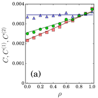
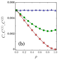
Figure 4: (a) Total clustering coefficient, $C$ (circles, green), single layer, $C^{(1)}$ (triangles, blue) and two layer, $C^{(2)}$ (squares, red), clustering coefficients for a two layer multiplex network with assortative inter layer degree correlations, joint degree distribution $P(q_{1},q_{2})=\rho\frac{1}{2}[(P(q_{1})+P(q_{2})]\delta_{q_{1},q_{2}}+(1-\rho)P(q_{1})P(q_{2})$, where $P(q)\propto q^{-\gamma}$, with $\gamma=2.9$ for $q\in[10,100]$. Each layer has $N=10^{4}$ vertices. For $\rho=0$ correlations are absent, while for $\rho=1$ degrees are perfectly correlated. Solid lines are expected theoretical values using Eqs. (11), (16), and (17). (b) Total $C$, single layer, $C^{(1)}$, and two layer, $C^{(2)}$, clustering coefficients for a two layer multiplex network with disassortative inter layer degree correlations, joint degree distribution $P(q_{1},q_{2})=\rho[(P(q_{1})\delta_{q_{2},0}+P(q_{2})\delta_{q_{1},0}]+(1-\rho)P(q_{1})P(q_{2})$, where $P(q)$ is a Poisson distribution with mean $50$. For $\rho=0$ correlations are absent, while for $\rho=1$ degrees are perfectly disjoint. Solid lines are expected theoretical values using Eqs. (11), (16), and (17).

To illustrate the importance of taking correlations into account, we compared our formulæ Eqs. (11)-(18) with measurements of synthetic networks. The results are summarized in Fig. 4. This shows that our method successfully accounts for the effects of broad degree distributions, and inter-layer correlations. In comparison, the Erdős-Rényi formulæ are generally only accurate for uncorrelated Erdős-Rényi layers and fail completely in the presence of strong correlations between layers.

IV Conclusions

In single layer networks, cycles are characterized by their length. In multiplex networks, there are many more possibilities. In particular, there is the possibility to switch between layers, and this must be accounted for. In this Paper we have introduced a classification for cycles in multiplex networks based on the number of edges in each layer, and the number of switches between layers. We further calculated the expected number of each type of cycle in a large random multiplex. Our results are valid for any multi-degree distribution, including distributions characterized by arbitrary degree correlations between layers. Interestingly, our formulæ show that the first and second order moments of the multi-degree distribution are sufficient to determine the statistics of cycles in large multiplex networks. The effect of correlations between a vertex’s degrees in different layers affects these statistics through the degree-degree moment $\langle q_{m}q_{n}\rangle$. Assortative correlations tend to increase the number of switches in cycles of a given length, while also increasing the total number of cycles. Disassortative correlations, on the other hand, may greatly reduce both the total number of cycles and the total number of switches within these cycles.

These results further allow us to give the expected clustering coefficients in multiplex networks. The possibility that a closed triangle may have edges in multiple layers requires a more detailed discrimination of clustering coefficients. We give a complete classification of the various possible clustering coefficients and give their expected values. Inter layer correlations again have a strong effect, significantly increasing or decreasing the mixed-layer clustering coefficients. These results give a much more precise view of cycles and clustering in multiplex networks than using the mean degree alone, and establish the proper baseline for comparison with real-world networks.

*

Appendix A The factor $R$ for longer cycles

The derivation given in the main body of this Paper is valid for $L\ll N$. If one wants to consider longer cycles, a more complex derivation is required, which we sketch here.

A.1 Cycles in only one layer

For orientation, we first outline the derivation for cycles within a single layer, which is identical to that for a single network, and follows the method used in Bianconi and Marsili (2005).

Consider selecting an arbitrary set of nodes from the network, of which $n_{q}$ have degree $q$. There are $\binom{N_{q}}{n_{q}}$ ways to select $n_{q}$ nodes, where $N_{q}=NP(q)$. We sum over all possible such sets and use a delta function to count only sets containing exactly $L$ nodes. There are $q(q-1)$ ways to select the edges which connect a node of degree $q$ in the cycle. Together these considerations mean we can write

$$R(N,L,P(q))=\\ N^{L}\!\sum_{\{n_{q}\}}\!\delta\!\left(\!\sum_{q}\!n_{q}\!-\!L\!\right)\!\prod_{q}\binom{N_{q}}{n_{q}}\!\left[\frac{q(q-1)}{N}\right]^{n_{q}}.$$ (26)

We can write the delta function in integral form, and after replacing the sum over sets $\{n_{q}\}$ with a sum over $n_{q}$ after the product, we have

$$R (N,L,P(q))$$

$$=\frac{N^{L}}{2\pi}\int\mathrm{d}x\,\prod_{q}\sum_{n_{q}=0}^{N_{q}}\binom{N_{q}}{n_{q}}\left[\frac{e^{ix}q(q-1)}{N}\right]^{n_{q}}e^{-ixL}$$

$$=\frac{N^{L}}{2\pi}\int\mathrm{d}x\,\prod_{q}\left[1+\frac{e^{ix}q(q-1)}{N}\right]^{N_{q}}e^{-ixL}.$$ (27)

Writing the product as a sum within an exponential, and recognising that as $N_{q}=NP(q)$, this gives an average over degree, we have

$$R(N,L,P(q))=\\ \frac{N^{L}}{2\pi}\int\mathrm{d}x\,\exp\left\{-ixL+N\left\langle\log\left[1+\frac{e^{ix}q(q-1)}{N}\right]\right\rangle\right\}.$$ (28)

To evaluate this integral, we assume the integrand to be strongly peaked around a certain value $x^{*}$. Let

$$\phi(x)=\frac{-ixL}{N}+\left\langle\log\left[1+\frac{e^{ix}q(q-1)}{N}\right]\right\rangle.$$ (29)

A local maximum of this function occurs at $x^{*}$ which is the solution of

$$\left\langle\frac{q(q-1)}{Ne^{-ix^{*}}+q(q-1)}\right\rangle=\frac{L}{N}.$$ (30)

The second derivative evaluated at $x^{*}$ is

$$\frac{\mathrm{d}^{2}\phi}{\mathrm{d}x^{2}}\Big{|}_{x=x^{*}}=-\left\langle\frac{q(q-1)}{[Ne^{-ix^{*}}+q(q-1)]^{2}}\right\rangle Ne^{-ix^{*}}.$$ (31)

These results can be used to replace $\phi(x)$ with a Taylor expansion about $x^{*}$ in Eq. (28). It has a simple Gaussian form that can easily be evaluated to give

$$R(N,L,P(q))=\\ \frac{N^{L}}{\sqrt{2\pi}}e^{N\phi(x^{*})}\left\{\left\langle\frac{q(q-1)}{[Ne^{-ix^{*}}+q(q-1)]^{2}}\right\rangle N^{2}e^{-ix^{*}}\right\}^{-1/2}.$$ (32)

To find an explicit expression, we must solve Eq. (30) and evaluate $\phi(x^{*})$ and hence Eq. (32).

In the case $L\ll N$, $Ne^{-ix}$ dominates $q(q-1)$, so that Eq. (30) becomes

$$\langle q(q-1)\rangle=Le^{-ix^{*}}$$ (33)

so that

$$N\phi(x^{*})=L+\log\left(\frac{\langle q(q-1)\rangle}{L}\right)^{L}$$ (34)

and

$$\left\{\left\langle\frac{q(q-1)}{[Ne^{-ix^{*}}+q(q-1)]^{2}}\right\rangle N^{2}e^{-ix^{*}}\right\}^{-1/2}=\frac{1}{\sqrt{L}}$$ (35)

giving

$$R(N,L,P(q))=\frac{N^{L}}{\sqrt{2\pi L}}e^{L}\left[\frac{\langle q(q-1)\rangle}{L}\right]^{L}=\frac{N^{L}}{L!}\langle q(q-1)\rangle^{L}$$ (36)

which when combined with Eqs. (2) and (6) gives exactly Eq. (9).

If instead we expand the lefthand side of Eq. (30) we find

$$\frac{s}{N}=\frac{\langle q(q-1)\rangle}{Ne^{-ix^{*}}}-\frac{\langle q^{2}(q-1)^{2}\rangle}{N^{2}e^{-2ix^{*}}}+...$$ (37)

and keeping the two leading terms , the solution is

$$e^{-ix^{*}} \approx\frac{\langle q(q-1)\rangle}{s}-\frac{\langle q^{2}(q-1)^{2}\rangle}{N\langle q(q-1)\rangle}$$ (38)

which can be substituted into Eqs. (29) and (32) to find the expected number of cycles when $L$ is not small compared with $N$ but $L\ll N^{2}$. The result will include dependence in $N$ and on higher moments of the degree distribution.

A.2 Cycles in two layers

Now we outline the derivation for general cycles in a two layer multiplex. We proceed in the same way, but now there are three sets of nodes $\{n^{(1)}_{q_{1},q_{2}}\}$ for the nodes connecting two edges in layer $1$, $\{n^{(2)}_{q_{1},q_{2}}\}$ for two edges in layer $2$, and $\{n^{(s)}_{q_{1},q_{2}}\}$ for the switches. We sum over all possible such sets, and use three delta functions to count only those whose total number of nodes (of all degrees) match $s_{ij}$. The combinatorial factor for the number of ways to select the three sets is

$$B_{n_{1},n_{2},n_{3}}^{N}=\frac{N!}{n_{1}!n_{2}!n_{3}!(N-n_{1}-n_{2}-n_{3})!}.$$ (39)

There are $q_{1}(q_{1}-1)$ ways to select the two edges connecting each of the $n^{(1)}_{q_{1},q_{2}}$ nodes, and similarly for $n^{(2)}_{q_{1},q_{2}}$, while for the $n^{(s)}_{q_{1},q_{2}}$ switches the factor is $q_{1}q_{2}$. These considerations give us

$$R(N,\mathbf{s},P(\mathbf{q}))=\sum_{\{n^{(1)}_{q_{1},q_{2}}\}}\delta\left(\sum_{q_{1},q_{2}}n^{(1)}_{q_{1},q_{2}}-s_{11}\right)\\ \sum_{\{n^{(2)}_{q_{1},q_{2}}\}}\delta\left(\sum_{q_{1},q_{2}}n^{(2)}_{q_{1},q_{2}}-s_{22}\right)\sum_{\{n^{(s)}_{q_{1},q_{2}}\}}\delta\left(\sum_{q_{1},q_{2}}n^{(s)}_{q_{1},q_{2}}-s_{12}\right)\\ \prod_{q_{1},q_{2}}\!\!B_{n^{(1)}_{q_{1},q_{2}},n^{(2)}_{q_{1},q_{2}},n^{(s)}_{q_{1},q_{2}}}^{N_{q_{1},q_{2}}}\!\!\!\!\left[q_{1}(q_{1}-1)\right]^{n^{(1)}_{q_{1},q_{2}}}\\ \times\left[q_{2}(q_{2}-1)\right]^{n^{(2)}_{q_{1},q_{2}}}\left[q_{1}q_{2}\right]^{n^{(s)}_{q_{1},q_{2}}}.$$ (40)

We can represent the delta function as an integral. Replacing the sums over sets $\{n^{(j)}_{q_{1},q_{2}}\}$ with sums over $n^{(j)}_{q_{1},q_{2}}$ after the product,

$$R(N,\mathbf{s},P(\mathbf{q}))=\frac{N^{L}}{(2\pi)^{3}}\int\mathrm{d}x_{1}\mathrm{d}x_{2}\mathrm{d}x_{3}\\ \exp\big{\{}ix_{1}(\sum_{q_{1},q_{2}}\!n^{(1)}_{q_{1},q_{2}}\!-\!s_{11})+ix_{2}(\sum_{q_{1},q_{2}}\!n^{(2)}_{q_{1},q_{2}}\!-\!s_{22})+\\ ix_{3}(\sum_{q_{1},q_{2}}\!n^{(2)}_{q_{1},q_{2}}\!-\!s_{12})\big{\}}\times\\ \prod_{q_{1},q_{2}}\sum_{n^{(1)}_{q_{1},q_{2}}=0}^{N_{q_{1},q_{2}}}\!\!\!\sum_{n^{(2)}_{q_{1},q_{2}}=0}^{N_{q_{1},q_{2}}\!-n^{(1)}_{q_{1},q_{2}}}\sum_{n^{(s)}_{q_{1},q_{2}}=0}^{N_{q_{1},q_{2}}\!-n^{(1)}_{q_{1},q_{2}}\!-n^{(2)}_{q_{1},q_{2}}}\!\!\!\!\!\!\!\!B_{n^{(1)}_{q_{1},q_{2}},n^{(2)}_{q_{1},q_{2}},n^{(s)}_{q_{1},q_{2}}}^{N_{q_{1},q_{2}}}\\ \!\left[\frac{q_{1}(q_{1}-1)}{N}\right]^{n^{(1)}_{q_{1},q_{2}}}\!\left[\frac{q_{2}(q_{2}-1)}{N}\right]^{n^{(2)}_{q_{1},q_{2}}}\!\left[\frac{q_{1}q_{2}}{N}\right]^{n^{(s)}_{q_{1},q_{2}}}.$$ (41)

Each sum can be completed succesively using the binomial identity. Finally converting the product into a sum within an exponential, and writing it as an expectation value we find

$$R(N,\mathbf{s},P(\mathbf{q}))=\frac{N^{L}}{(2\pi)^{3}}\int\mathrm{d}x_{1}\,\mathrm{d}x_{2}\mathrm{d}\,x_{3}\exp\{N\phi({\bf{x}})\}.$$ (42)

where

$$\phi({\bf{x}})=\frac{1}{N}\left[\log\left(\frac{y_{1}}{N}\right)^{s_{11}}+\log\left(\frac{y_{2}}{N}\right)^{s_{22}}+\log\left(\frac{y_{3}}{N}\right)^{s_{12}}\right]+\\ \bigg{\langle}\log\left[1+\frac{b_{1}}{y_{1}}+\frac{b_{2}}{y_{2}}+\frac{b_{3}}{y_{3}}\right]\bigg{\rangle}$$ (43)

and $y_{j}=Ne^{-ix_{j}}$ and $b_{1}=q_{1}(q_{1}-1)$, $b_{2}=q_{2}(q_{2}-1)$, and $b_{3}=q_{1}q_{2}$.

As before, we expand $\phi({\bf{x}})$ about the local maximum $\bf{x}^{*}$ which is the simultaneous solution of

$$\frac{s_{11}}{N} =\left\langle\frac{b_{1}}{y_{1}^{*}[1+b_{1}/y_{1}^{*}+b_{2}/y_{2}^{*}+b_{3}/y_{3}^{*}]}\right\rangle$$ (44)

$$\frac{s_{22}}{N} =\left\langle\frac{b_{2}}{y_{2}^{*}[1+b_{1}/y_{1}^{*}+b_{2}/y_{2}^{*}+b_{3}/y_{3}^{*}]}\right\rangle$$ (45)

$$\frac{s_{12}}{N} =\left\langle\frac{b_{3}}{y_{3}^{*}[1+b_{1}/y_{1}^{*}+b_{2}/y_{2}^{*}+b_{3}/y_{3}^{*}]}\right\rangle.$$ (46)

The Taylor expansion requires the second order derivatives:

$$\phi_{jj}\equiv\frac{\partial^{2}\phi}{\partial x_{j}^{2}}\Big{|}_{\bf{x}^{*}} =-\frac{1}{y_{j}^{*}}\left\langle\frac{b_{j}(1+b_{k}/y_{k}^{*}+b_{l}/y_{l}^{*})}{(1+b_{1}/y_{1}^{*}+b_{2}/y_{2}^{*}+b_{3}/y_{3}^{*})^{2}}\right\rangle$$ (47)

$$\phi_{jk}\equiv\frac{\partial^{2}\phi}{\partial x_{j}x_{k}}\Big{|}_{\bf{x}^{*}} =\frac{1}{y_{j}^{*}y_{k}^{*}}\left\langle\frac{b_{j}b_{k}}{(1+b_{1}/y_{1}^{*}+b_{2}/y_{2}^{*}+b_{3}/y_{3}^{*})^{2}}\right\rangle$$ (48)

where the subscripts $j,k,l$ each take one of the values $1,2,3$. Substituting the second order Taylor expansion of $\phi(\bf{x})$ around $\bf{x}^{*}$ into Eq. (42) yields a more complex integral than in the single layer case, but its evaluation is still straightforward,

$$R(N,\mathbf{s},P(\mathbf{q}))=\frac{N^{L}e^{N\phi({\bf{x}}^{*})}}{(2\pi N)^{3/2}}\left[\phi_{11}\phi_{22}\phi_{33}\right.\\ \left.-\phi_{11}\phi_{23}^{2}-\phi_{22}\phi_{13}^{2}-\phi_{33}\phi_{12}^{2}-2\phi_{12}\phi_{13}\phi_{23}\right]^{-1/2}.$$ (49)

To evaluate $R(N,\mathbf{s},P(\mathbf{q}))$ for a given distribution, one solves Eqs. (44)-(46), evaluates Eqs. (47) and (48) and substitutes into Eq. (49)).

For $L\ll N$ we can neglect $\mathcal{O}(1/N)$, giving $y_{1}^{*}=N\langle b_{1}\rangle/s_{11}$ and similar expressions for $y_{2}^{*}$ and $y_{3}^{*}$. The cross derivatives $\phi_{12}$, $\phi_{13}$, and $\phi_{23}$ vanish, and we recover Eq. (7). For larger $L$, dependence on $N$ will remain, and there will be dependence on higher moments of the degree distribution.

References

• Rinaldi et al. (2001) S. M. Rinaldi, J. P. Peerenboom,  and T. K. Kelly, “Identifying, understanding, and analyzing critical infrastructure interdependencies,” IEEE Control Syst. Mag. 21, 11–25 (2001).
• Huang et al. (2013) X. Huang, I. Vodenska, S. Havlin,  and H. E. Stanley, Sci. Rep. 3, 1219 (2013).
• De Domenico et al. (2014) M. De Domenico, A. Solé-Ribalta, S. Gómez,  and A. Arenas, “Navigability of interconnected networks under random failures,” Proc. Natl. Acad. Sci. U.S.A. 111, 8351–8356 (2014)arXiv:1306.0519 .
• Pocock et al. (2012) M. J. O. Pocock, D. M. Evans,  and J. Memmott, “The robustness and restoration of a network of ecological networks,” Science 335, 973–976 (2012).
• Boccaletti et al. (2014) S. Boccaletti, G. Bianconi, R. Criado, C. I. Del Genio, J. Gómez-Gardeñes, M. Romance, I. Sendiña-Nadal, Z. Wang,  and M. Zanin, “The structure and dynamics of multilayer networks,” Phys. Rep. 544, 1–122 (2014).
• Kivela et al. (2014) M. Kivela, A. Arenas, M. Barthelemy, J. P. Gleeson, Y. Moreno,  and M. A. Porter, “Multilayer networks,” Journal of Complex Networks 2, 203–271 (2014).
• De Domenico et al. (2016) M. De Domenico, C. Granell, M. A. Porter,  and A. Arenas, “The physics of multilayer networks,” arXiv preprint arXiv:1604.02021  (2016).
• Baxter et al. (2012) G. J. Baxter, S. N. Dorogovtsev, A. V. Goltsev,  and J. F.F. Mendes, “Avalanche collapse of interdependent networks,” Phys.Rev. Lett. 109, 248701 (2012).
• Baxter et al. (2016) G. J. Baxter, D. Cellai, S. N. Dorogovtsev, A. V. Goltsev,  and J. F. F. Mendes, “A unified approach to percolation processes on multiplex networks,” in Interconnected Networks (Springer, 2016) pp. 101–123.
• Cozzo et al. (2015) E. Cozzo, M. Kivelä, M. De Domenico, A. Solé-Ribalta, A. Arenas, S. Gómez, M. A. Porter,  and Y. Moreno, “Structure of triadic relations in multiplex networks,” New J. Phys. 17, 073029 (2015).
• Newman (2003) M. E. J. Newman, “The structure and function of complex networks,” SIAM Review 45, 167–256 (2003)arXiv:cond-mat/0303516 .
• Bianconi and Capocci (2003) G. Bianconi and A. Capocci, “Number of loops of size hh in growing scale-free networks,” Phys. Rev. Lett. 90, 078701 (2003).
• Bollobás and Riordan (2003) B. Bollobás and O. M. Riordan, “Mathematical results on scale-free random graphs,” in Handbook of Graphs and Networks: From the Genome to the Internet, edited by S. Bornholdt and H. G. Schuster (Wiley-VCH, Weinheim, 2003) pp. 1–34.
• Melnik et al. (2011) S. Melnik, A. Hackett, M. A. Porter, P. Mucha,  and J. Gleeson, “The unreasonable effectiveness of tree-based theory for networks with clustering,” Phys. Rev. E 83, 036112 (2011).
• Kim and Goh (2013) J. Y. Kim and K. Goh, “Coevolution and correlated multiplexity in multiplex networks,” Phys. Rev. Lett. 111, 058702 (2013).
• Hackett et al. (2016) A. Hackett, D. Cellai, S. Gómez, A. Arenas,  and J. P. Gleeson, “Bond percolation on multiplex networks,” Physical Review X 6, 021002 (2016).
• Bollobás (2001) Béla Bollobás, Random Graphs, 2nd ed. (Cambridge University Press, Cambridge, 2001).
• Harary and Manvel (1971) F. Harary and B. Manvel, “On the number of cycles in a graph,” Math. Slovaca 21, 55–63 (1971).
• Abouelaoualim et al. (2010) A. Abouelaoualim, Das, W. Fernandez de la Vega, M. Karpinski, Y. Manoussakis, C. A. Martinhon,  and R. Saad, “Cycles and paths in edge-colored graphs with given degrees,” J. Graph Theory 64, 63–86 (2010).
• Wang and Desmedt (2011) Y. Wang and Y. Desmedt, “Edge-colored graphs with applications to homogeneous faults,” Inform. Process. Lett. 111, 634–641 (2011).
• Jain (2004) K. Jain, “Security based on network topology against the wiretapping attack,” IEEE wirel. commun. 11, 68–71 (2004).
• Bender and Canfield (1978) E. A. Bender and E. R. Canfield, “The asymptotic number of labeled graphs with given degree sequences,” J. Combinator. Theor. Series A 24, 296 (1978).
• Bollobás (1980) B. Bollobás, “A probabilistic proof of an asymptotic formula for the number of labelled regular graphs,” Eur. J. Combinator. 1, 311 (1980).
• Bianconi and Marsili (2005) G. Bianconi and M. Marsili, “Loops of any size and hamilton cycles in random scale-free networks,” J. Stat. Mech. Theor. Exp. 2005, P06005 (2005).
• Bianconi and Marsili (2006) G. Bianconi and M. Marsili, “Effect of degree correlations on the loop structure of scale-free networks,” Phys. Rev. E 73, 066127+ (2006).