On fixed gain recursive estimators with discontinuity in the parameters

Abstract

In this paper we estimate the expected tracking error of a fixed gain stochastic approximation scheme. The underlying process is not assumed Markovian, a mixing condition is required instead. Furthermore, the updating function may be discontinuous in the parameter.

MSC 2010 subject classification: Primary: 62L20; secondary: 93E15, 93E35

Keywords: adaptive control, stochastic gradient, fixed gain, recursive estimators, parameter discontinuity, mixing processes, non-Markovian dynamics

1 Introduction

Let $\mathbb{N}:=\{0,1,2,\ldots\}$. We are interested in stochastic approximation procedures where a parameter estimate ${\theta}_{t}$, $t\in\mathbb{N}$ is updated by a recursion of the form

$${\theta}_{t+1}={\theta}_{t}+\gamma_{t+1}H({\theta}_{t},X_{t+1}),\ t\in\mathbb{N},$$ (1)

starting from some guess $\theta_{0}$. Here $X_{t}$ is a stationary signal, $\gamma_{t}$ is a sequence of real numbers and $H(\cdot,\cdot)$ is a given functional. The most common choices are $\gamma_{t}=1/t$ (decreasing gain) and $\gamma_{t}:=\lambda$ (fixed gain). The former family of procedures is aimed to converge to $\theta^{*}$ with $G(\theta^{*})=0$ where $G(\theta):=EH(\theta,X_{t})$. The latter type of procedures is supposed to “track” $\theta^{*}$, even when the system dynamics is (slowly) changing.

In most of the related literature the error analysis of (1) was carried out only in the case where $H$ is (Lipschitz-)continuous in $\theta$. This restrictive hypothesis fails to accommodate discontinuous procedures which are common in practice, e.g. the signed regressor, signed error and sign-sign algorithms (see [3], [7], [8]) or the Kohonen algorithm (see [27, 1]). Recently, the decreasing gain case was investigated in [9] for controlled Markov chains and the procedure (1) was shown to converge almost surely under appropriate assumptions, without requiring continuity of $H$. We refer to [9] for a review of the relevant literature and for examples.

The purpose of the present article is an exploration of the case where $X_{t}$ has possibly non-Markovian dynamics. We consider fixed gain procedures and weaken continuity of $H$ to continuity in the sense of conditional expectations, see (6) below, compare also to condition $\mathbf{H4}$ in [9].

We follow the methodology of the papers [19, 14, 17] which are based on the concept of $L$-mixing, coming from [12]. Our arguments work under a modification of the original definition of $L$-mixing, see Section 2. We furthermore assume a certain asymptotic forgetting property, see Assumption 3.4. We manage to estimate the tracking error for (1), see our main result, Theorem 3.6 in Section 3.

At this point we would like to make comparisons with another important reference, [28], where no Markovian or continuity assumptions were made, certain averaging properties of the driving process were required instead. It follows from Subsection 4.2 of [28] that almost sure convergence of a decreasing gain procedure can be guaranteed under the $\alpha$-mixing property of the driving process, see e.g. [6] about various mixing concepts. It seems that establishing the $L$-mixing property is often relatively simple while $\alpha$-mixing is rather stringent and difficult to prove. In addition, our present work provides explicit estimates for the error. See Section 4 for examples illustrating the scope of Theorem 3.6.

Section 5 reports simulations showing that the theoretical estimate is in accordance with numerical results. Proofs for Sections 2 and 3 are relegated to Section 6.

2 $L$-mixing and conditional $L$-mixing

Estimates for the error of stochastic approximation schemes like (1) can be proved under various ergodicity assumptions on the driving process. It is demonstrated in [14] and [17] that the concept of $L$-mixing (see its definition below in the present section) is sufficiently strong for this purpose. An appealing feature of $L$-mixing is that it can easily be applied in non-Markovian contexts as well, see Section 4.

It turns out, however, that for discontinuous updating functions $H$ the arguments of [14, 17] break down. To tackle discontinuities, we introduce a new concept of mixing here, which is of interest on its own right.

Throughout this paper we are working on a probability space $(\Omega,\mathcal{F},P)$ that is equipped with a discrete-time filtration $\mathcal{F}_{n}$, $n\in\mathbb{N}$ as well as with a decreasing sequence of sigma-fields $\mathcal{F}_{n}^{+}$, $n\in\mathbb{N}$ such that $\mathcal{F}_{n}$ is independent of $\mathcal{F}_{n}^{+}$, for all $n$.

Expectation of a random variable $X$ will be denoted by $EX$. For any $m\geq 1$, for any $\mathbb{R}^{m}$-valued random variable $X$ and for any $1\leq p<\infty$, let us set $\|X\|_{p}:=\sqrt[p]{E|X|^{p}}$. We denote by $L^{p}$ the set of $X$ satisfying $\|X\|_{p}<\infty$. The indicator function of a set $A$ will be denoted by $1_{A}$.

We now present the class of $L$-mixing processes which were introduced in [12]. This concept proved to be extremely useful in solving certain hard problems of system identification, see e.g. [15, 16, 13, 18, 30].

Fix an integer $N\geq 1$ and let $D\subset\mathbb{R}^{N}$ be a set of parameters. A measurable function $X:\mathbb{N}\times D\times\Omega\to\mathbb{R}^{m}$ is called a random field. We will drop dependence on $\omega\in\Omega$ and use the notation $X_{t}(\theta)$, $t\in\mathbb{N}$, $\theta\in D$.

For any $r\geq 1$, a random field $X_{t}(\theta)$, $t\in\mathbb{N}$, $\theta\in D$ is called bounded in $L^{r}$ if

$$M_{r}(X):=\sup_{\theta\in D}\sup_{t\in\mathbb{N}}\|X_{t}(\theta)\|_{r}<\infty.$$ (2)

For an $L^{r}$-bounded $X_{t}(\theta)$, define also the quantities

$$\gamma_{r}(\tau,X):=\sup_{\theta\in D}\sup_{t\geq\tau}\|X_{t}(\theta)-E[X_{t}(\theta)|\mathcal{F}_{t-\tau}^{+}]\|_{r},\ \tau\geq 1,$$

and

$$\Gamma_{r}(X):=\sum_{\tau=1}^{\infty}\gamma_{r}(\tau,X).$$ (3)

For some $r\geq 1$, a random field $X_{t}(\theta)$ is called uniformly $L$-mixing of order $r$ (ULM-$r$) if it is bounded in $L^{r}$; for all $\theta\in D$, $X_{t}(\theta)$, $t\in\mathbb{N}$ is adapted to $\mathcal{F}_{t}$, $t\in\mathbb{N}$; and $\Gamma_{r}(X)<\infty$. Here uniformity refers to the parameter $\theta$. Furthermore, $X_{t}(\theta)$ is called uniformly $L$-mixing if it is uniformly $L$-mixing of order $r$ for all $r\geq 1$.

In the case of a single stochastic process (which corresponds to the case where the parameter set $D$ is a singleton) we apply the terminology “$L$-mixing process of order $r$” and “$L$-mixing process”.

Remark 2.1.

The $L$-mixing property shows remarkable stability under various operations, this is why it proved to be a versatile tool in the analysis of stochastic systems, see [14, 17, 15, 16, 13, 18, 30]. If $F$ is a Lipschitz function and $X_{t}(\theta)$ is ULM-$r$ then $F(X_{t}(\theta))$ is also ULM-$r$, by (33) in Lemma 6.1 below. Actually, if $F$ is such that $|F(x)-F(y)|\leq K(1+|x|^{k}+|y|^{k})|x-y|$ for all $x,y\in\mathbb{R}$ with some $k,K>0$ then $F(X_{t}(\theta))$ is uniformly $L$-mixing whenever $X_{t}(\theta)$ is, see Proposition 2.4 of [30]. Stable linear filters also preserve the $L$-mixing property, see [12]. Proving that $F(X_{t}(\theta))$ is $L$-mixing for discontinuous $F$ is more delicate, see Section 4 for helpful techniques.

Other mixing conditions could alternatively be used. Some of these are inherited by arbitrary measurable functions of the respective processes (e.g. $\phi$-mixing, see Section 7.2 of [6]). However, they are considerably difficult to verify while $L$-mixing (and its conditional version to be defined below) is relatively simple to check, see also the related remarks on page 2129 of [18].

Recall that, for any family $Z_{i}$, $i\in I$ of real-valued random variables, $\mathrm{ess.}\sup_{i\in I}Z_{i}$ denotes a random variable that is an almost sure upper bound for each $Z_{i}$ and it is a.s. smaller than or equal to any other such bound. Such an object is known to exist, independently of the cardinality of $I$, and it is a.s. unique, see e.g. Proposition VI.1.1. of [29].

Now we define conditional $L$-mixing, inspired by (2) and (3). Let $X_{t}(\theta)$, $t\in\mathbb{N}$, $\theta\in D$ be a random field bounded in $L^{r}$ for some $r\geq 1$ and define, for each $n\in\mathbb{N}$,

$$M^{n}_{r}(X) := \mathrm{ess}\sup_{\theta\in D}\sup_{t\in\mathbb{N}}E^{1/r}[|X_{n+t}(\theta)|^{r}\big{|}\mathcal{F}_{n}],$$

$$\gamma^{n}_{r}(\tau,X) := \mathrm{ess}\sup_{\theta\in D}\sup_{t\geq\tau}E^{1/r}[|X_{n+t}(\theta)-E[X_{n+t}(\theta)|\mathcal{F}_{n+t-\tau}^{+}\vee\mathcal{F}_{n}]|^{r}\big{|}\mathcal{F}_{n}],\ \tau\geq 1,$$

$$\Gamma^{n}_{r}(X) := \sum_{\tau=1}^{\infty}\gamma^{n}_{r}(\tau,X).$$

For some $s,r\geq 1$, we call $X_{t}(\theta)$, $t\in\mathbb{N}$, $\theta\in D$ uniformly conditionally $L$-mixing of order $(r,s)$ (abbreviation: UCLM-$(r,s)$) if it is $L^{r}$-bounded; $X_{t}(\theta)$, $t\in\mathbb{N}$ is adapted to $\mathcal{F}_{t}$, $t\in\mathbb{N}$ for all $\theta\in D$ and the sequences $M^{n}_{r}(X)$, $\Gamma^{n}_{r}(X)$, $n\in\mathbb{N}$ are bounded in $L^{s}$. When the UCLM-$(r,s)$ property holds for all $r,s\geq 1$ then we simply say that the random field is uniformly conditionally $L$-mixing. In the case of stochastic processes (when $D$ is a singleton) the terminology “conditionally $L$-mixing process of order $(r,s)$” (respectively, conditionally $L$-mixing process) will be used.

Remark 2.2.

Note that if $\mathcal{F}_{0}$ is trivial and $X_{t}(\theta)$ is UCLM-$(r,1)$ then it is also ULM-$r$. Indeed, in that case

$$M_{r}(X)=M_{r}^{0}(X),\quad\Gamma_{r}(X)=\Gamma_{r}^{0}(X).$$

For non-trivial $\mathcal{F}_{0}$, however, no such implication holds.

Remark 2.3.

If $F$ is a Lipschitz function and $X_{t}(\theta)$ is UCLM-$(r,1)$ then $F(X_{t}(\theta))$ is also UCLM-$(r,1)$, by Lemma 6.1 below. Conditional versions of the arguments in Lemma 6.2 show that if $X_{t}(\theta)$ is UCLM-$(rp,1)$ and $Y_{t}(\theta)$ is UCLM-$(rq,1)$ (where $1/p+1/q=1$) then

$$M^{n}_{r}(XY) \leq M^{n}_{rp}(X)M^{n}_{rq}(Y),$$ (4)

$$\Gamma^{n}_{r}(XY) \leq 2M^{n}_{rp}(X)\Gamma^{n}_{rq}(Y)+2\Gamma^{n}_{rp}(X)M^{n}_{rq}(Y).$$ (5)

We now present another concept, a surrogate for continuity in $\theta\in D$. We say that the random field $X_{t}(\theta)\in L^{1}$, $t\in\mathbb{N}$, $\theta\in D$ satisfies the conditional Lipschitz-continuity (CLC) property if there is a deterministic $K>0$ such that, for all $\theta_{1},\theta_{2}\in D$ and for all $n\in\mathbb{N}$,

$$E\left[|X_{n+1}(\theta_{1})-X_{n+1}(\theta_{2})|\,\Big{|}\mathcal{F}_{n}\right]\leq K|\theta_{1}-\theta_{2}|,\mbox{ a.s.}$$ (6)

Pathwise discontinuities of $\theta\to X_{n}(\theta)$ can often be smoothed out and (6) can be verified by imposing some conditions on the one-step conditional distribution of $X_{n+1}$ given $\mathcal{F}_{n}$, see Assumption 4.3 and Lemma 4.7 below.

Remark 2.4.

We comment on the differences between condition $\mathbf{H4}$ of [9] and our CLC property. Assume that $X$ is stationary and Markovian. On one hand, $\mathbf{H4}$ of [9] stipulates that, for $\delta>0$

$$\sup_{\theta\in D_{c}}E\left[\sup_{\theta^{\prime}\in D_{c},\ |\theta-\theta^{\prime}|\leq\delta}|H(\theta,X_{1})-H(\theta^{\prime},X_{1})|\right]\leq K\delta^{\alpha}$$ (7)

for any compact $D_{c}\subset D$ with some $K>0$ (that may depend on $D_{c}$) and with some $0<\alpha\leq 1$ (independent of $D_{c}$). On the other hand, CLC is equivalent to

$$\sup_{\theta,\theta^{\prime}\in D,\ |\theta-\theta^{\prime}|\leq\delta}E\left[\left|H(\theta,X_{1})-H(\theta^{\prime},X_{1})\right|\,\big{|}X_{0}=x\right]\leq K\delta.$$ (8)

for $\mathrm{Law}(X_{0})$-almost every $x$. Clearly, (7) allows Hölder-continuity (i.e. $\alpha<1$) while (8) requires Lipschitz-continuity. In the case $\alpha=1$ (7) is not comparable to CLC though both express a kind of “continuity in the average”.

The main results of our paper require a specific structure for the sigma-algebras which facilitates to deduce properties of conditional $L$-mixing processes from those of “unconditional” ones. More precisely, we rely on the crucial Doob-type inequality in Theorem 2.5 below. This could probably be proved for arbitrary sigma-algebras but only at the price of redoing all the tricky arguments of [12] in a more difficult context. We refrain from this since Theorem 2.5 can accommodate most models of practical importance. Let $\mathbb{Z}$ denote the set of integers.

Theorem 2.5.

Fix $r>2$, $n\in\mathbb{N}$. Assume that, for all $t\in\mathbb{N}$, $\mathcal{F}_{t}=\sigma(\varepsilon_{j},\ j\in\mathbb{N},\ j\leq t)$, $\mathcal{F}_{t}^{+}:=\sigma(\varepsilon_{j},\ j>t)$ for some i.i.d. sequence $\varepsilon_{j}$, $j\in\mathbb{Z}$ with values in some Polish space $\mathcal{X}$. Let $W_{t}$, $t\in\mathbb{N}$ be a conditionally $L$-mixing process of order $(r,1)$, satisfying $E[W_{t}|\mathcal{F}_{n}]=0$ a.s. for all $t\geq n$. Let $m>n$ and let $b_{t}$, $n<t\leq m$ be deterministic numbers. Then we have

$$E^{1/r}\left[\max_{n<t\leq m}\left|\sum_{s=n+1}^{t}b_{s}W_{s}\right|^{r}\big{|}\mathcal{F}_{n}\right]\leq C_{r}\left(\sum_{s=n+1}^{m}b_{s}^{2}\right)^{1/2}\sqrt{{M}_{r}^{n}(W)\Gamma_{r}^{n}(W)},$$ (9)

almost surely, where $C_{r}$ is a deterministic constant depending only on $r$ but independent of $n,m$.

The proof is reported in Section 6.

3 Fixed gain stochastic approximation

Let $N\geq 1$ be an integer and let $\mathbb{R}^{N}$ be the Euclidean space with norm $|x|:=\sqrt{\sum_{i=1}^{N}x_{i}^{2}}$, $x\in\mathbb{R}^{N}$. Let $D\subset\mathbb{R}^{N}$ be a bounded (nonempty) open set representing possible system parameters. Let $H:D\times\mathbb{R}^{m}\to\mathbb{R}^{N}$ be a bounded measurable function. We assume throughout this section that for all $t\in\mathbb{N}$, $\mathcal{F}_{t}=\sigma(\varepsilon_{j},\ j\in\mathbb{N},\ j\leq t)$, $\mathcal{F}_{t}^{+}:=\sigma(\varepsilon_{j},\ j>t)$ for some i.i.d. sequence $\varepsilon_{j}$, $j\in\mathbb{Z}$ with values in some Polish space $\mathcal{X}$, in particular the condition on the sigma algebras in the statement of Theorem 2.5 holds.

Let

$$X_{t}:=g(\varepsilon_{t},\varepsilon_{t-1},\ldots),\ t\in\mathbb{N},$$ (10)

with some fixed measurable function $g:\mathcal{X}^{-\mathbb{N}}\to\mathbb{R}^{m}$. Clearly, $X$ is a (strongly) stationary $\mathbb{R}^{m}$-valued process, see Lemma 10.1 of [24].

Remark 3.1.

We remark that, in the present setting, the CLC property holds if, for all $\theta_{1},\theta_{2}\in D$,

$$E\left[|H(\theta_{1},X_{1})-H(\theta_{2},X_{1})|\,\Big{|}\mathcal{F}_{0}\right]\leq K|\theta_{1}-\theta_{2}|,\mbox{ a.s.},$$

due to the fact that the law of $(X_{k+1},\varepsilon_{k},\varepsilon_{k-1},\ldots)$ is the same as that of $(X_{1},\varepsilon_{0},\varepsilon_{-1},\ldots)$, for all $k\in\mathbb{Z}$.

Define $G(\theta):=EH(\theta,X_{0})$. Note that, by stationarity of $X$, $G(\theta)=EH(\theta,X_{t})$ for all $t\in\mathbb{N}$. We need some stability hypotheses formulated in terms of an ordinary differential equation related to $G$.

Assumption 3.2.

On $D$, the function $G$ is twice continuously differentiable and bounded, together with its first and second derivatives.

Fix $\lambda>0$. Under Assumption 3.2, the equation

$$\dot{y}_{t}=\lambda G(y_{t}),\quad y_{s}=\xi,$$ (11)

has a unique solution for each $s\geq 0$ and $\xi\in D$, on some (finite or infinite) interval $[s,v(s,\xi))$ with $v(s,\xi)>s$. We will denote this solution by $y(t,s,\xi)$, $t\in[s,v(s,\xi))$. Let $D_{1}\subset D$ such that for all $\xi\in D_{1}$ we have $y(t,0,\xi)\in D$ for any $t\geq 0$. We denote

$$\phi(D_{1})=\{u\in D:\,u=y(t,0,\xi),\text{ for some }t\geq 0,\ \xi\in D_{1}\}.$$

The $\varepsilon$-neighbourhood of a set $D_{1}$ is denoted by $S(D_{1},\varepsilon)$, i.e.

$$S(D_{1},\varepsilon)=\{u\in\mathbb{R}^{N}:|u-\theta|<\varepsilon\text{ for some }\theta\in D_{1}\}.$$

We remark that, under Assumption 3.2, the function $y(t,s,\xi)$ is continuously differentiable in $\xi$.

Notice that all the above observations would be true under weaker hypotheses than those of Assumption 3.2. However, the proof of Lemma 6.5 below requires the full force of Assumption 3.2, see [17].

Assumption 3.3.

There exist open sets

$$\emptyset\neq D_{\xi}\subset D_{y}\subset D_{\theta}\subset D_{\overline{y}}\subset D$$

such that $\phi(D_{\xi})\subset D_{y}$, $S(D_{y},d)\subset D_{\theta}$ for some $d>0$ and $\phi(D_{\theta})\subset D_{\overline{y}}$, $S(D_{\overline{y}},d^{\prime})\subset D$ for some $d^{\prime}>0$. The ordinary differential equation (11) is exponentially asymptotically stable with respect to initial perturbations, i.e. there exist $C^{*}>0,\alpha>0$ such that, for each $\lambda$ sufficiently small, for all $0\leq s\leq t$, $\xi\in D$

$$\left|\frac{\partial}{\partial{\xi}}y(t,s,\xi)\right|\leq C^{*}e^{-\lambda\alpha(t-s)}.$$ (12)

We furthermore assume that there is $\theta^{*}\in D$ such that

$$G(\theta^{*})=0.$$ (13)

It follows from $\phi(D_{\xi})\subset D_{y}$ and (12) that $\theta^{*}$ actually lies in the closure of $D_{y}$ and that there is only one $\theta^{*}$ satisfying (13).

While Assumptions 3.2, 3.3 pertained to a deterministic equation, our next hypothesis is of a stochastic nature.

Assumption 3.4.

For all $n\in\mathbb{N}$,

$$E\left[\sup_{\vartheta\in D}\sum_{k=n}^{\infty}\left|E[H(\vartheta,X_{k+1})|\mathcal{F}_{n}]-G(\vartheta)\right|\right]<\infty$$ (14)

Remark 3.5.

Assumption 3.4 expresses a certain kind of “forgetting”: for $k$ large, $E[H(\vartheta,X_{k+1})|\mathcal{F}_{n}]$ is close to $G(\vartheta)=EH(\theta,X_{k+1})|_{\theta=\vartheta}$ in $L^{1}$, uniformly in $\vartheta$ and the convergence is fast enough so that the sum in (14) is finite. In other words, this is again a kind of mixing property.

In certain cases, the validity of Assumption 3.4 indeed follows from $L$-mixing. Let $X_{t}$, $t\in\mathbb{N}$ be $L$-mixing of order $1$ and let $x\to H(\theta,x)$ be Lipschitz-continuous with a Lipschitz constant $L^{\dagger}$ that is independent of $\theta$. We claim that Assumption 3.4 holds under these conditions. Indeed, for every $\vartheta\in D$

$$\sum_{k=n}^{\infty}E\left|E\left[H(\vartheta,X_{k+1})|\mathcal{F}_{n}\right]-E[H(\theta,X_{k+1})]|_{\theta=\vartheta}\right| \leq$$

$$\sum_{k=n}^{\infty}\left|E\left[H(\vartheta,X_{k+1})|\mathcal{F}_{n}\right]-E\left[H(\vartheta,E[X_{k+1}|\mathcal{F}^{+}_{n}])|\mathcal{F}_{n}\right]\right| +$$

$$\sum_{k=n}^{\infty}\left|E\left[H(\theta,E[X_{k+1}|\mathcal{F}^{+}_{n}])\right]|_{\theta=\vartheta}-E[H(\theta,X_{k+1})]|_{\theta=\vartheta}\right| \leq$$

$$2L^{\dagger}\sum_{k=n}^{\infty}\left|X_{k+1}-E[X_{k+1}|\mathcal{F}^{+}_{n}]\right|$$

noting that

$$E\left[H(\vartheta,E[X_{k+1}|\mathcal{F}^{+}_{n}])|\mathcal{F}_{n}\right]=E\left[H(\theta,E[X_{k+1}|\mathcal{F}^{+}_{n}])\right]|_{\theta=\vartheta},$$

by independence of $\mathcal{F}_{n}$ and $\mathcal{F}_{n}^{+}$. Hence

$$E\left[\sup_{\vartheta\in D}\sum_{k=n}^{\infty}\left|E[H(\vartheta,X_{k+1})|\mathcal{F}_{n}]-G(\vartheta)\right|\right]\leq 2L^{\dagger}\Gamma_{1}(X)<\infty.$$

Assumption 3.4 can also be verified in certain cases where $H$ is discontinuous, see Section 4.

We now state the main result of our article.

Theorem 3.6.

Let $H(\theta,X_{t})$ be UCLM-$(r,1)$ for some $r>2$, satisfying the CLC property (see (6) above). Let Assumptions 3.2, 3.3 and 3.4 be in force. For some $\xi\in D_{\xi}$, define the recursive procedure

$$\theta_{0}:=\xi,\quad{\theta}_{t+1}={\theta}_{t}+\lambda H({\theta}_{t},X_{t+1}),$$ (15)

with some $\lambda>0$. Define also its “averaged” version,

$$z_{0}:=\xi,\quad z_{t+1}=z_{t}+\lambda G(z_{t}).$$ (16)

Let $d,d^{\prime}$ in Assumption 3.3 be large enough and let $\lambda$ be small enough. Then $\theta_{t},z_{t}\in D_{\theta}$ for all $t$ and there is a constant $C$, independent of $t\in\mathbb{N}$ and of $\lambda$, such that

$$E\left|{\theta}_{t}-z_{t}\right|\leq C\lambda^{1/2},\ t\in\mathbb{N}.$$

An important consequence of the main theorem is provided as follows.

Corollary 3.7.

Under the conditions of Theorem 3.6, there is $t_{0}(\lambda)\in\mathbb{N}$ such that

$$E\left|{\theta}_{t}-\theta^{*}\right|\leq C\lambda^{1/2},\ t\geq t_{0}(\lambda).$$

Furthermore, $t_{0}(\lambda)\leq C^{\circ}\ln(1/\lambda)/\lambda$ for some $C^{\circ}>0$ .

The proofs of Theorem 3.6 and Corollary 3.7 are postponed to Section 6.

Remark 3.8.

Our current investigations were motivated by [17] where not only the random field $H(\theta,X_{t})$ was assumed $L$-mixing, but also its “derivative field”

$$\frac{H(\theta_{1},X_{t})-H(\theta_{2},X_{t})}{\theta_{1}-\theta_{2}},\ t\in\mathbb{N},\ \theta_{1},\theta_{2}\in D,\ \theta_{1}\neq\theta_{2}.$$ (17)

As shown in Section 3 of [12], the latter hypothesis necessarily implies the continuity (in $\theta$) of $H(\theta,X_{t})$. For our purposes such an assumption is thus too strong. We are able to drop continuity at the price of modifying the $L$-mixing concept, as explained in Section 2 above.

We point out that our results complement those of [17] even in the case where $H$ is Lipschitz-continuous (in that case the CLC property of our paper obviously holds). In [17], the derivative field (17) was assumed to be $L$-mixing. In the present paper we do not need this hypothesis (but we assume conditional $L$-mixing of order $(r,1)$ for some $r>2$ instead of $L$-mixing).

4 Examples

The present section serves to illustrate the power of Theorem 3.6 above by exhibiting processes $X_{t}$ and functions $H$ to which that theorem applies.

The (conditional) $L$-mixing property can be verified for arbitrary bounded measurable functionals of Markov processes with the Doeblin condition (see [20]) and this could probably be extended to a larger family of Markov processes using ideas of [2] or [22]. We prefer not to review the corresponding methods here but to present some non-Markovian examples because they demonstrate better the advantages of our approach over the existing literature.

In Subsection 4.1 linear processes (see e.g. Subsection 3.2 of [21]) with polynomial autocorrelation decay are considered, while Subsection 4.2 presents a class of Markov chains in a random environment with contractive properties.

4.1 Causal linear processes

Assumption 4.1.

Let $\varepsilon_{j}$, $j\in\mathbb{Z}$ be a sequence of independent, identically distributed real-valued random variables such that $E|\varepsilon_{0}|^{\zeta}<\infty$ for some $\zeta\geq 2$ and $E\varepsilon_{0}=0$. We set $\mathcal{F}_{n}=\sigma(\varepsilon_{i},i\leq n)$, and $\mathcal{F}^{+}_{n}=\sigma(\varepsilon_{i},i>n)$ for each $n\in\mathbb{Z}$. Let us define the process

$$X_{t}:=\sum_{j=0}^{\infty}a_{j}\varepsilon_{t-j},\quad t\in\mathbb{Z},$$ (18)

where $a_{j}\in\mathbb{R}$, $j\in\mathbb{N}$. We assume $a_{0}\neq 0$ and

$$|a_{j}|\leq C_{1}(j+1)^{-\beta},\ j\in\mathbb{N},$$

for some constants $C_{1}>0$ and $\beta>1/2$.

Note that the series (18) converges a.s. (by Kolmogorov’s theorem, see e.g. Chapter 4 of [24]). As a warm-up, we now check the conditional $L$-mixing property for $X$.

Lemma 4.2.

Let Assumption 4.1 be in force. If $\beta>3/2$ then the process $X_{t}$, $t\in\mathbb{N}$ is conditionally $L$-mixing of order $(\zeta,1)$.

Proof.

We have, for $t\in\mathbb{N}$,

$$E^{1/\zeta}[|X_{t}|^{\zeta}|\mathcal{F}_{0}] \leq E^{1/\zeta}\left[2^{\zeta-1}|\sum_{j=0}^{t-1}a_{j}\varepsilon_{t-j}|^{\zeta}\big{|}\mathcal{F}_{0}\right]+E^{1/\zeta}\left[2^{\zeta-1}|\sum_{j=t}^{\infty}a_{j}\varepsilon_{t-j}|^{\zeta}\big{|}\mathcal{F}_{0}\right]$$

$$\leq 2^{\frac{\zeta-1}{\zeta}}\sum_{j=0}^{t-1}|a_{j}|\|\varepsilon_{t-j}\|_{\zeta}+2^{\frac{\zeta-1}{\zeta}}\sum_{j=t}^{\infty}|a_{j}\varepsilon_{t-j}|$$

using the simple inequality $(x+y)^{\zeta}\leq 2^{\zeta-1}(x^{\zeta}+y^{\zeta})$, $x,y\geq 0$; properties of the norm $\|\cdot\|_{\zeta}$; independence of $\varepsilon_{j}$, $j\geq 1$ from $\mathcal{F}_{0}$ and $\mathcal{F}_{0}$-measurability of $\varepsilon_{j}$, $j\leq 0$. Hence

$$E^{1/\zeta}[|X_{t}|^{\zeta}|\mathcal{F}_{0}] \leq 2^{\frac{\zeta-1}{\zeta}}\|\varepsilon_{0}\|_{\zeta}\sum_{j=0}^{\infty}|a_{j}|+2^{\frac{\zeta-1}{\zeta}}\sum_{j=0}^{\infty}C_{1}(t+j+1)^{-\beta}|\varepsilon_{-j}|$$

$$\leq 2^{\frac{\zeta-1}{\zeta}}\|\varepsilon_{0}\|_{\zeta}\sum_{j=0}^{\infty}|a_{j}|+2^{\frac{\zeta-1}{\zeta}}\sum_{j=0}^{\infty}C_{1}(j+1)^{-\beta}|\varepsilon_{-j}|$$

$$\leq C_{2}\left[1+\sum_{j=0}^{\infty}|\varepsilon_{-j}|(j+1)^{-\beta}\right],$$

for some $C_{2}>0$. Note that the latter bound is independent of $t$. Similar estimates prove that, for all $n\geq 0$,

$$M^{n}_{\zeta}(X)\leq C_{2}\left[1+\sum_{j=0}^{\infty}|\varepsilon_{n-j}|(j+1)^{-\beta}\right].$$

The right-hand side has the same law for all $n$ and it is in $L^{1}$ since $\beta>1$. This implies that the sequence $M^{n}_{\zeta}(X)$, $n\in\mathbb{N}$ is bounded in $L^{1}$.

For $1\leq m$ and for any $t\in\mathbb{Z}$, define

$$X_{t,m}^{+}:=\sum_{j=0}^{m-1}a_{j}\varepsilon_{t-j},$$

and, for $t\geq m$, let

$$X^{\circ}_{t,m}:=X_{t,m}^{+}+\sum_{j=t}^{\infty}a_{j}\varepsilon_{t-j}.$$

Notice that $E[X_{t}|\mathcal{F}_{t-m}^{+}\vee\mathcal{F}_{0}]=X_{t,m}^{\circ}$ and, by independence of $\varepsilon_{j}$, $j\geq 1$ from $\mathcal{F}_{0}$,

$$E[|X_{t}-X_{t,m}^{\circ}|^{\zeta}\big{|}\mathcal{F}_{0}]=\left\|\sum_{j=m}^{t-1}a_{j}\varepsilon_{t-j}\right\|_{\zeta}^{\zeta} \leq$$ (19)

$$C_{3}E\left(\sum_{j=m}^{t-1}a^{2}_{j}\varepsilon^{2}_{t-j}\right)^{\zeta/2} \leq$$

$$C_{3}\left(\sum_{j=m}^{t-1}\|a^{2}_{j}\varepsilon^{2}_{t-j}\|_{\zeta/2}\right)^{\zeta/2} \leq$$

$$C_{3}\left(C_{1}^{2}\sum_{j=m}^{\infty}(1+j)^{-2\beta}\|\varepsilon_{0}\|_{\zeta}^{2}\right)^{\zeta/2}\leq\left(C_{3}^{\prime}m^{-2\beta+1}\right)^{\zeta/2},$$

with some constants $C_{3},C_{3}^{\prime}>0$, using the Marczinkiewicz-Zygmund inequality. Define $b_{m}:=\sqrt{C_{3}^{\prime}}m^{-\beta+1/2}$. An analogous estimate gives $\gamma^{n}_{\zeta}(m,X)\leq b_{m}$ for all $n\in\mathbb{N}$. Since $\sum_{m=1}^{\infty}b_{m}<\infty$ by $\beta>3/2$, $\Gamma^{n}_{\zeta}(X)$ is actually bounded by a constant, uniformly in $n$. ∎

We also need in the sequel that the law of the driving noise is smooth enough. This is formulated in terms of the characteristic function $\phi$ of $\varepsilon_{0}$.

Assumption 4.3.

We require that

$$\int_{\mathbb{R}}|\phi(u)|\,du<\infty.$$ (20)

Remark 4.4.

Assumption 4.3 implies the existence of a (continuous and bounded) density $f$ for the law of $\varepsilon_{0}$ (with respect to the Lebesgue measure). Indeed, $f$ is the inverse Fourier transform of $\phi$:

$$f(x)=\frac{1}{2\pi}\int_{\mathbb{R}}\phi(u)e^{-iux}\,du,\ x\in\mathbb{R}.$$

Conversely, if the law of $\varepsilon_{0}$ has a twice continuously differentiable density $f$ such that $f^{\prime}$, $f^{\prime\prime}$ are integrable over $\mathbb{R}$ then (20) holds. The latter observation follows by standard Fourier-analytic arguments.

Lemma 4.5.

Let Assumptions 4.1 and 4.3 be in force. Then the law of $X_{0}$ (resp. $X^{+}_{0,m}$) has a density $f_{\infty}$ (resp. $f_{m}$) with respect to the Lebesgue measure. Moreover, there is a constant $\tilde{K}>0$ such that

$$\sup_{m\in\mathbb{N}\cup\{\infty\}}\sup_{x\in\mathbb{R}}f_{m}(x)\leq\tilde{K}.$$

Proof.

Denote by $\phi_{m}$ the characteristic function of $X^{+}_{0,m}$. Since $|\phi(u)|\leq 1$ for all $u$, we see that

$$|\phi_{m}(u)|=\left|\prod_{j=0}^{m-1}\phi(a_{j}u)\right|\leq|\phi(a_{0}u)|,$$ (21)

which implies, by applying an inverse Fourier transform, the existence of $f_{m}$ and the estimate

$$|f_{m}(x)|\leq\frac{1}{2\pi}\int_{\mathbb{R}}|\phi(a_{0}u)|\,du=:\tilde{K}<\infty,\mbox{ for all }x\in\mathbb{R},\ m\geq 1,$$

by Assumption 4.3. As $X_{0,m}^{+}$ tends to $X_{0}$ in probability when $m\to\infty$, $\phi_{m}(u)$ tends to $\phi_{\infty}(u)$ for all $u$, where $\phi_{\infty}$ is the characteristic function of $X_{0}$. The integrable bound (21) is uniform in $m$, so $f_{\infty}$ exists and the dominated convergence theorem implies that $f_{m}(x)$ tends to $f_{\infty}(x)$, for all $x\in\mathbb{R}$. The result follows. ∎

Let $D\subset\mathbb{R}^{N}$ be a bounded open set. In the sequel we consider functionals of the form

$$H(\theta,x):=\sum_{j=1}^{M}g_{j}(\theta,x)1_{\{x\in I_{j}(\theta)\}},\ x\in\mathbb{R},\ \theta\in D,$$ (22)

where the $g_{j}$ are bounded and Lipschitz-continuous functions (jointly in the two variables) and the intervals $I_{j}(\theta)$ are of the form $(-\infty,h_{j}(\theta))$, $(h_{j}(\theta),\infty)$ or $(h^{1}_{j}(\theta),h^{2}_{j}(\theta))$ with $h_{j},h^{1}_{j},h^{2}_{j}:D\to\mathbb{R}$ Lipschitz-continuous functions.

Remark 4.6.

The intervals $I_{j}(\theta)$ can also be closed or half-closed and the results below remain valid, this is clear from the proofs. In the one-dimensional case, the signed regressor, signed error, sign-sign and Kohonen algorithms all have an updating function of the form (22), see [7], [8], [27], [1]. For simplicity, we only treat the one-dimensional setting (i.e. $x\in\mathbb{R}$) in the present paper but we allow $D$ to be multidimensional.

Lemma 4.7.

Let Assumptions 4.1 and 4.3 be in force. Then a random field $H(\theta,X_{t})$, $t\in\mathbb{N}$, $\theta\in D$ as in (22) satisfies the CLC property (6).

Proof.

It suffices to consider $H(\theta,X_{1})=g(\theta,X_{1})1_{\{X_{1}\in I(\theta)\}}$ with $g$ Lipschitz-continuous, bounded and $I$ of the form $(-\infty,h(\theta))$, $(h(\theta),\infty)$ or $(h^{1}(\theta),h^{2}(\theta))$ with $h,h^{1},h^{2}$ Lipschitz. We only prove the first case, the other cases being similar. Recall also Remark 3.1.

Denoting by $C_{4}$ a Lipschitz-constant for $g$ and by $C_{5}$ an upper bound for $|g|$, we get the estimate

$$|H(\theta_{1},X_{1})-H(\theta_{2},X_{1})| \leq$$

$$|1_{\{X_{1}<h(\theta_{1})\}}g(\theta_{1},X_{1})-1_{\{X_{1}<h(\theta_{1})\}}g(\theta_{2},X_{1})| +$$

$$|1_{\{X_{1}<h(\theta_{1})\}}g(\theta_{2},X_{1})-1_{\{X_{1}<h(\theta_{2})\}}g(\theta_{2},X_{1})| \leq$$

$$C_{4}|\theta_{1}-\theta_{2}|+C_{5}|1_{\{X_{1}<h(\theta_{1})\}}-1_{\{X_{1}<h(\theta_{2})\}}| \leq$$

$$C_{4}|\theta_{1}-\theta_{2}|+C_{5}\left(1_{\{X_{1}\in[h(\theta_{1}),h(\theta_{2}))\}}+1_{\{X_{1}\in[h(\theta_{2}),h(\theta_{1}))\}}\right).$$

We may and will assume $h(\theta_{1})<h(\theta_{2})$. It suffices to prove that

$$P\left(X_{1}\in[h(\theta_{1}),h(\theta_{2}))|\mathcal{F}_{0}\right)\leq C_{6}|\theta_{1}-\theta_{2}|$$

with a suitable $C_{6}>0$. Noting that the density of $a_{0}\varepsilon_{1}$ is $x\to(1/|a_{0}|)f(x/a_{0})$, we have

$$P\left(X_{1}\in[h(\theta_{1}),h(\theta_{2}))|\mathcal{F}_{0}\right) = \int_{h(\theta_{1})-\sum_{j=1}^{\infty}a_{j}\varepsilon_{1-j}}^{h(\theta_{2})-\sum_{j=1}^{\infty}a_{j}\varepsilon_{1-j}}\frac{1}{|a_{0}|}{f}(x/a_{0})\,dx\leq$$

$$\frac{1}{|a_{0}|}K_{0}|h(\theta_{1})-h(\theta_{2})| \leq \frac{1}{|a_{0}|}K_{0}C_{7}|\theta_{1}-\theta_{2}|,$$

where $K_{0}$ is an upper bound for $f$ (see Remark 4.4) and $C_{7}$ is a Lipschitz constant for $h$. This completes the proof. ∎

Theorem 4.8.

Let Assumptions 4.1 and 4.3 be in force. Let $H$ be of the form specified in (22). Let $\zeta\geq 2r$ and let $\beta$ satisfy $\beta>4r+1/2$. Then the random field $H(\theta,X_{t})$, $t\in\mathbb{N}$, $\theta\in D$ is UCLM-$(r,1)$.

Proof.

We may and will assume

$$H(\theta,X_{t})=g(\theta,X_{t})1_{\{X_{t}\in I(\theta)\}}$$

with some bounded Lipschitz function $g$ and with some interval $I(\theta)$ of the type as in (22). As $H$ is bounded, ${M}_{r}^{n}(H)$, $n\in\mathbb{N}$ is trivially a bounded sequence in $L^{1}$.

In view of (4), (5), it suffices to establish that $1_{\{X_{t}\in I(\theta)\}}$, $t\in\mathbb{N}$ is UCLM-$(2r,1)$ (since $g(\theta,X_{t})$, $1_{\{X_{t}\in I(\theta)\}}$ are bounded and $g(\theta,X_{t})$ is UCLM-$(2r,1)$, by $\zeta\geq 2r$, Lemma 4.2 and Remark 2.3). We show this for $I(\theta)=(-\infty,h(\theta))$ with $h$ Lipschitz-continuous as other types of intervals can be handled similarly.

As

$$\mathrm{Law}(X_{t+n},\,t\in\mathbb{N},\,\varepsilon_{n-j},\,j\in\mathbb{N})=\mathrm{Law}(X_{t},\,t\in\mathbb{N},\,\varepsilon_{-j},\,j\in\mathbb{N})$$

for all $n\in\mathbb{N}$, we may reduce the proof to estimations for the case $n:=0$. Let us start with

$$\left|1_{\{X_{t,m}^{\circ}<h(\theta)\}}-1_{\{X_{t}<h(\theta)\}}\right| =$$

$$1_{\{X_{t,m}^{\circ}<h(\theta),X_{t}\geq h(\theta)\}}+1_{\{X_{t}<h(\theta),X_{t,m}^{\circ}\geq h(\theta)\}} \leq$$

$$1_{\{X_{t}\in(h(\theta)-\eta_{m},h(\theta)+\eta_{m})\}}+1_{\{|X_{t,m}^{\circ}-X_{t}|\geq\eta_{m}\}},$$

for all $\eta_{m}>0$. We will choose a suitable $\eta_{m}$ later. Using Lemma 4.5 and the conditional Markov inequality we obtain

$$E\left[|1_{\{X_{t,m}^{\circ}<h(\theta)\}}-1_{\{X_{t}<h(\theta)\}}|^{2r}|\mathcal{F}_{0}\right] \leq$$

$$C_{8}P(X_{t}\in(h(\theta)-\eta_{m},h(\theta)+\eta_{m})|\mathcal{F}_{0}) +$$

$$C_{8}P(|X_{t,m}^{\circ}-X_{t}|\geq\eta_{m}|\mathcal{F}_{0}) \leq$$

$$2C_{8}\tilde{K}\eta_{m}+C_{8}E\left[|X_{t}-X_{t,m}^{\circ}|\big{|}\mathcal{F}_{0}\right]/\eta_{m},$$ (23)

with some constant $C_{8}$, noting that powers of indicators are themselves indicators and that the conditional density of $X_{t}$ with respect to $\mathcal{F}_{0}$ is $x\to f_{t}(x-\sum_{j=t}^{\infty}a_{j}\varepsilon_{t-j})$ and the latter is $\leq\tilde{K}$ by Lemma 4.5. Using (19), the second term in (23) is bounded by $C_{8}\sqrt{C_{3}^{\prime}}m^{-\beta+1/2}/\eta_{m}$ hence it is reasonable to choose $\eta_{m}:=1/m^{(\beta-1/2)/2}$, which leads to

$$E^{1/2r}\left[|1_{\{X_{t,m}^{\circ}<h(\theta)\}}-1_{\{X_{t}<h(\theta)\}}|^{2r}\big{|}\mathcal{F}_{0}\right]\leq C_{9}/m^{(\beta-1/2)/(4r)},$$

with some $C_{9}>0$. Notice that $X_{t,m}^{\circ}$ is $\mathcal{F}^{+}_{t-m}\vee\mathcal{F}_{0}$-measurable. Lemma 6.1 implies that $\gamma_{2r}(X,m)\leq 2C_{9}/m^{(\beta-1/2)/(4r)}$. As $(\beta-1/2)/(4r)>1$ by our hypotheses, we obtain the UCLM-$(2r,1)$ property for $1_{\{X_{t}\in I(\theta)\}}$. ∎

Remark 4.9.

When $\varepsilon_{0}$ has moments of all orders then one can reduce the lower bound $4r+1/2$ for $\beta$ in Theorem 4.8 to $r+1/2$. Indeed, in this case $g(\theta,X_{t})$ is UCLM-$(q,1)$ for arbitrarily large $q$ by Lemma 4.2 and Remark 2.3 so it suffices to show the UCLM-$(r^{\prime},1)$ property for $1_{\{X_{t}\in I(\theta)\}}$ for some $r^{\prime}>r$ that can be arbitrarily close to $r$ (and not for $r^{\prime}=2r$ as in Theorem 4.8). The estimate of the above proof can be improved to

$$E\left[|1_{\{X_{t,m}^{\circ}<h(\theta)\}}-1_{\{X_{t}<h(\theta)\}}|^{r^{\prime}}|\mathcal{F}_{0}\right] \leq$$

$$2C_{8}\tilde{K}\eta_{m}+C_{8}E\left[|X_{t}-X_{t,m}^{\circ}|^{q}\big{|}\mathcal{F}_{0}\right]/\eta_{m}^{q},$$

for arbitrarily large $q$. Choosing $\eta_{m}:=1/m^{[q(\beta-1/2)]/(q+1)}$, we arrive at

$$E^{1/r^{\prime}}\left[|1_{\{X_{t,m}^{\circ}<h(\theta)\}}-1_{\{X_{t}<h(\theta)\}}|^{r^{\prime}}\big{|}\mathcal{F}_{0}\right]\leq C_{9}/m^{[q(\beta-1/2)]/[(q+1)r^{\prime}]}.$$

Let $\beta>r+1/2$. If $r^{\prime}>r$ is chosen close enough to $r$ and $q$ is chosen large enough then $[q(\beta-1/2)]/[(q+1)r^{\prime}]>1$ which shows the UCLM-$(r,1)$ property for $H(\theta,X_{t})$.

Lemma 4.10.

Let Assumptions 4.1 and 4.3 be in force, let $\beta>3/2$. Then, for all $n\in\mathbb{N}$,

$$E\left[\sum_{k=n}^{\infty}\sup_{\vartheta\in D}\left|E\left[H(\vartheta,X_{k+1})|\mathcal{F}_{n}\right]-G(\vartheta)\right|\right]\leq C_{10}$$

with some fixed $C_{10}<\infty$. That is, Assumption 3.4 holds.

Proof.

We need to estimate

$$\sum_{k=n}^{\infty}\left[\left|E\left[g(\vartheta,X_{k+1})1_{\{X_{k+1}<h(\vartheta)\}}|\mathcal{F}_{n}\right]-E[g(\theta,X_{k+1})1_{\{X_{k+1}<h(\theta)\}}]|_{\theta=\vartheta}\right|\right],$$

where $h:D\to\mathbb{R}$ is Lipschitz-continuous and $g$ is a bounded, Lipschitz-continuous function with a bound $C_{11}$ for $|g|$ and with Lipschitz constant $C_{12}$. It suffices to prove

$$E\left[\sup_{\vartheta\in D}\sum_{k=1}^{\infty}\left|E\left[g(\vartheta,X_{0})1_{\{X_{0}<h(\vartheta)\}}|\mathcal{F}_{-k}\right]-E[g(\theta,X_{0})1_{\{X_{0}<h(\theta)\}}]|_{\theta=\vartheta}\right|\right]<\infty,$$

since the law of $(X_{0},\varepsilon_{-k},\varepsilon_{-k-1},\ldots)$ equals that of $(X_{n+k},\varepsilon_{n},\varepsilon_{n-1},\ldots)$, for all $k\geq 1$, $n\in\mathbb{Z}$. We can estimate a given term in the above series as follows:

$$\left|E\left[g(\vartheta,X_{0})1_{\{X_{0}<h(\vartheta)\}}|\mathcal{F}_{-k}\right]-E[g(\theta,X_{0})1_{\{X_{0}<h(\theta)\}}]|_{\theta=\vartheta}\right| \leq$$

$$\left|E\left[g(\vartheta,X_{0})1_{\{X_{0}<h(\vartheta)\}}|\mathcal{F}_{-k}\right]-E[g(\vartheta,X_{0,k}^{+})1_{\{X_{0,k}^{+}<h(\vartheta)\}}|\mathcal{F}_{-k}]\right| +$$

$$\left|E[g(\theta,X_{0,k}^{+})1_{\{X_{0,k}^{+}<h(\theta)\}}]|_{\theta=\vartheta}-E[g(\theta,X_{0})1_{\{X_{0}<h(\theta)\}}]|_{\theta=\vartheta}\right| \leq$$

$$C_{12}E\left[|X_{0}-X_{0,k}^{+}|\Big{|}\mathcal{F}_{-k}\right]+C_{11}E\left[|1_{\{X_{0,k}^{+}<h(\vartheta)\}}-1_{\{X_{0}<h(\vartheta)\}}|\Big{|}\mathcal{F}_{-k}\right] +$$

$$C_{12}|X_{0}-X_{0,k}^{+}|+C_{11}E\left[|1_{\{X_{0,k}^{+}<h(\theta)\}}-1_{\{X_{0}<h(\theta)\}}|\right]|_{\theta=\vartheta}$$ (24)

noting that $E[g(\theta,X_{0,k}^{+})1_{\{X_{0,k}^{+}<h(\theta)\}}]|_{\theta=\vartheta}=E[g(\vartheta,X_{0,k}^{+})1_{\{X_{0,k}^{+}<h(\vartheta)\}}|\mathcal{F}_{-k}]$. The first and third terms on the right-hand side of (24) are equal and they are $\leq C_{13}k^{-\beta+1/2}$ with some $C_{13}>0$, by the proof of Lemma 4.2, hence their sum (when $k$ goes from $1$ to infinity) is finite. The expression in the second term of (24) can be estimated as

$$E\left[|1_{\{X_{0,k}^{+}<h(\vartheta)\}}-1_{\{X_{0}<h(\vartheta)\}}|\Big{|}\mathcal{F}_{-k}\right] \leq$$

$$P\left(X_{0}\in\left(h(\vartheta)-\sum_{j=k}^{\infty}a_{j}\varepsilon_{-j},h(\vartheta)+\sum_{j=k}^{\infty}a_{j}\varepsilon_{-j}\right)|\mathcal{F}_{-k}\right) \leq$$

$$2\tilde{K}\left|\sum_{j=k}^{\infty}a_{j}\varepsilon_{-j}\right|,$$ (25)

noting that the conditional density of $X_{0}$ with respect to $\mathcal{F}_{-k}$ is $x\to f_{k}\left(x-\sum_{j=k}^{\infty}a_{j}\varepsilon_{-j}\right)$ and this is bounded by $\tilde{K}$, using Lemma 4.5. Since (25) is independent of $\vartheta$, a similar estimate guarantees that

$$E\left[|1_{\{X_{0,k}^{+}<h(\theta)\}}-1_{\{X_{0}<h(\theta)\}}|\right]|_{\theta=\vartheta}\leq 2\tilde{K}\left|\sum_{j=k}^{\infty}a_{j}\varepsilon_{-j}\right|.$$

Note that the upper estimates obtained so far do not depend on $\vartheta$. It follows that, even taking supremum in $\vartheta\in D$, the expectations of the second and fourth terms on the right-hand side of (24) are both $\leq C_{14}k^{(-\beta+1/2)}$ with some $C_{14}>0$. As $\beta>3/2$, the infinite sum of these terms is finite, too, finishing the proof of the present lemma. ∎

Assumption 4.11.

Let $f$ satisfy

$$|f(x)|\leq\widehat{C}e^{-\widehat{\delta}|x|}\mbox{ for all }x\in\mathbb{R},$$ (26)

with some $\widehat{C},\widehat{\delta}>0$

Assumption 4.12.

Let

$$\int_{\mathbb{R}}u^{2}|\phi_{u}|\,du<\infty$$ (27)

hold.

Remark 4.13.

Clearly, Assumption 4.11 implies that $\varepsilon_{0}$ has finite moments of all orders. Note also that Assumption 4.12 implies Assumption 4.3.

Remark 4.14.

If $f$ is four times continuously differentiable such that $f^{\prime}$, $f^{\prime\prime}$, $f^{\prime\prime\prime}$, $f^{\prime\prime\prime\prime}$ are integrable then (27) holds, compare to Remark 4.4 above.

Lemma 4.15.

Let Assumptions 4.1, 4.11 and 4.12 hold. Let the functions $g_{i}$, $h^{1}_{i}$, $h^{2}_{i}$, $h_{i}$ of (22) be twice continuously differentiable with bounded first and second derivatives. Then $G(\theta):=EH(\theta,X_{0})$ is bounded and twice continuously differentiable with bounded first and second derivatives, i.e. Assumption 3.2 holds.

Proof.

We may and will assume that

$$H(\theta,x)=1_{\{x<h(\theta)\}}g(\theta,x)$$

with $h$ Lipschitz-continuous, $g$ bounded and Lipschitz-continuous. $G$ is bounded since $g$ is. We proceed to establish its differentiability and the boundedness of its derivatives.

Recall that

$$\phi_{\infty}(u)=\prod_{j=0}^{\infty}\phi(a_{j}u),\ u\in\mathbb{R},$$

where $\phi_{\infty}$ is the characteristic function of $X_{0}$ and the product converges pointwise. Since $|\phi(u)|\leq 1$ for all $u$, (27) implies that

$$\int_{\mathbb{R}}u^{2}|\phi_{\infty}(u)|\,du<\infty.$$

Clearly, this implies $\int_{\mathbb{R}}|u\phi_{\infty}(u)|\,du<\infty$ and $\int_{\mathbb{R}}|\phi_{\infty}(u)|\,du<\infty$ as well (since $\phi_{\infty}$ is bounded, being a Fourier transform). Now one can directly show, using the inverse Fourier transform, that $f_{\infty}$, the density of the law of $X_{0}$, is twice continuously differentiable.

Inequality (26) implies that $\phi$ has a complex analytic extension in a strip around $\mathbb{R}$. Since the sequence $a_{j}$, $j\in\mathbb{N}$ is bounded, there is even a strip such that $u\to\phi(a_{j}u)$ is analytic in it, for all $j\in\mathbb{N}$, thus $\phi_{\infty}$ is also analytic there. Then so are $-iu\phi_{\infty}(u)$ and $-u^{2}\phi_{\infty}(u)$. These being integrable, we get that their inverse Fourier transforms, $f_{\infty}^{\prime}$ and $f_{\infty}^{\prime\prime}$, satisfy

$$|f_{\infty}^{\prime}(x)|+|f_{\infty}^{\prime\prime}(x)|\leq\tilde{C}e^{-\tilde{\delta}|x|}\mbox{ for all }x\in\mathbb{R},$$ (28)

with some $\tilde{C},\tilde{\delta}>0$, see e.g. Theorem 11.9.3 of [25]. In particular, $f_{\infty}^{\prime},f_{\infty}^{\prime\prime}$ are integrable.

For notational simplicity we consider only the case $N=1$, i.e. $D\subset\mathbb{R}$. Using the change of variable $y=x-h(\theta)$, we see that

$$EH(\theta,X_{0})=\int_{\mathbb{R}}g(\theta,x)1_{\{x<h(\theta)\}}f_{\infty}(x)\,dx=\int_{-\infty}^{0}g(\theta,y+h(\theta))f_{\infty}(y+h(\theta))\,dy.$$

We calculate $\partial_{\theta}g(\theta,y+h(\theta))f_{\infty}(y+h(\theta))$:

$$[\partial_{1}g(\theta,y+h(\theta))+\partial_{2}g(\theta,y+h(\theta))h^{\prime}(\theta)]f_{\infty}(y+h(\theta))+g(\theta,y+h(\theta))f_{\infty}^{\prime}(y+h(\theta))h^{\prime}(\theta),$$

where $\partial_{1}$ (resp. $\partial_{2}$) denote differentiation with respect to the first (resp. second) variable. As $f_{\infty}$ (resp. $f_{\infty}^{\prime}$) satisfy (26) (resp. (28)) and $g,\partial_{1}g,\partial_{2}g,h^{\prime}$ are bounded, the dominated convergence theorem implies that

$$\partial_{\theta}EH(\theta,X_{0}) =$$

$$\int_{-\infty}^{0}[\partial_{1}g(\theta,y+h(\theta))+\partial_{2}g(\theta,y+h(\theta))h^{\prime}(\theta)]f_{\infty}(y+h(\theta))\,dy +$$

$$\int_{-\infty}^{0}g(\theta,y+h(\theta))f_{\infty}^{\prime}(y+h(\theta))h^{\prime}(\theta)\,dy =$$

$$\int_{\mathbb{R}}1_{\{x<h(\theta)\}}[\partial_{1}g(\theta,x)+\partial_{2}g(\theta,x)h^{\prime}(\theta)]f_{\infty}(x)\,dx +$$

$$\int_{\mathbb{R}}1_{\{x<h(\theta)\}}g(\theta,x)f_{\infty}^{\prime}(x)h^{\prime}(\theta)\,dx,$$

where both integrals are clearly bounded in $\theta$. Similar calculations involving the second derivatives of $g,h,f_{\infty}$ show that $\partial_{\theta}^{2}EH(\theta,X_{0})$ exists and it is bounded in $\theta$. ∎

The following corollary summarizes our findings in the present section.

Corollary 4.16.

Let $H$ be of the form (22) such that $g_{j},h_{j},h^{1}_{j},h^{2}_{j}$ are twice continuously differentiable with bounded first and second derivatives. Let Assumptions 4.1, 4.11 and 4.12 hold and assume $\beta>5/2$. Then Theorem 3.6 applies to the random field $H(\theta,X_{t})$, $t\in\mathbb{N}$, $\theta\in D$, provided that Assumption 3.3 holds.

Proof.

Recalling 4.13 and 4.9, this corollary follows from the results of the present section. ∎

Assumptions 4.11 and 4.12 apply, in particular, when $\varepsilon_{0}$ is Gaussian. There does not seem to be a general condition guaranteeing the validity of Assumption 3.3: this needs checking in every concrete application of Theorem 3.6.

4.2 Markov chains in a random environment

If $\beta\leq 5/2$ in the setting of Subsection 4.1 above then Corollary 4.16 cannot be established with our methods. Hence $X_{t}$ cannot be a “long memory processes” in the sense of [21]. In this subsection we show that it is nonetheless possible to apply Theorem 3.6 to important classes of random fields that are driven by a long memory process, see Example 4.18 below.

Let $\varepsilon^{1}_{t}$, $t\in\mathbb{Z}$, $\varepsilon^{2}_{t}$, $t\in\mathbb{Z}$ be i.i.d. real-valued sequences, independent of each other.

Assumption 4.17.

We denote $\chi_{t}:=(\varepsilon^{1}_{j+t})_{j\in\mathbb{Z}}$, for each $t\in\mathbb{Z}$. Let $F:\mathbb{R}^{\mathbb{Z}}\times\mathbb{R}\times\mathbb{R}^{m}\to\mathbb{R}^{m}$ be a measurable function such that, for all $w\in\mathbb{R}^{\mathbb{Z}}$, $s\in\mathbb{R}$,

$$|F(w,s,z_{1})-F(w,s,z_{2})|\leq\rho|z_{1}-z_{2}|,$$

for all $z_{1},z_{2}\in\mathbb{R}^{m}$ with some $0<\rho<1$. Furthermore, there is $x\in\mathbb{R}^{m}$ such that for all $w\in\mathbb{R}^{\mathbb{Z}}$ and for all $s\in\mathbb{R}$,

$$|F(w,s,x)-x|\leq C(1+|s|)$$

and $E|\varepsilon_{0}^{2}|^{r}<\infty$ for some $r>2$.

Fix $x\in\mathbb{R}$ as in Assumption 4.17 and define, for all $t\in\mathbb{Z}$, $\tilde{X}^{t}_{0}:=x$, and for $j\geq 0$,

$$\tilde{X}^{t}_{j+1}:=F(\chi_{t},\varepsilon_{t}^{2},\cdot)\circ F(\chi_{t-1},\varepsilon_{t-1}^{2},\cdot)\circ\cdots F(\chi_{t-j},\varepsilon_{t-j}^{2},\cdot)(x).$$

Standard arguments (such as Proposition 5.1 of [5]) show that $\tilde{X}_{j}^{t}$ converges almost surely as $j\to\infty$. Define

$$X_{t}:=\lim_{j\to\infty}\tilde{X}^{t}_{j}.$$

Then $X_{t}$, $t\in\mathbb{Z}$ is clearly a stationary process, satisfying

$$X_{t+1}=F(\chi_{t+1},\varepsilon_{t+1}^{2},X_{t}),\ t\in\mathbb{Z}.$$

When freezing the values of $\varepsilon_{t}^{1}$, $t\in\mathbb{Z}$, the $X_{t}$ defined above is an (inhomogeneous) Markov chain driven by the noise sequence $\varepsilon_{t}^{2}$, $t\in\mathbb{Z}$. Hence $X_{t}$ is a Markov chain in a random environment (the latter is driven by $\varepsilon_{t}^{1}$, $t\in\mathbb{Z}$).

Example 4.18.

Let $\varepsilon_{i}^{2}$, $i\in\mathbb{Z}$ be i.i.d. with $E|\varepsilon_{0}^{2}|^{r}<\infty$ for some $r>2$. Let $E\varepsilon_{0}^{1}=0$, $E(\varepsilon_{0}^{1})^{2}<\infty$. Let $Y_{t}:=\sum_{j=0}^{\infty}a_{j}\varepsilon_{t-j}^{1}$, $t\in\mathbb{Z}$ for some $a_{j}$, $j\in\mathbb{N}$ with $\sum_{j=0}^{\infty}a_{j}^{2}<\infty$. The series converges almost surely. Let $h_{1},h_{2}:\mathbb{R}\to\mathbb{R}$ be bounded measurable and fix $-1<\kappa,\rho<1$. The construction sketched above provides the existence of a process $X_{t}$ satisfying

$$X_{t+1}=\kappa X_{t}+\rho e^{h_{1}(Y_{t+1})}h_{2}(\varepsilon_{t+1}^{1})+\sqrt{1-\rho^{2}}e^{h_{1}(Y_{t+1})}\varepsilon_{t+1}^{2}.$$

This is an instance of stochastic volatility models where $h_{1}(Y)$ corresponds to the log-volatility of an asset and $X$ is the increment of the log-price of the same asset. Note that $Y$ may have a slow autocorrelation decay (e.g. $a_{j}\sim j^{-\beta}$ with any $\beta>1/2$ is possible). This model resembles the “fractional stochastic volatility model” of [4, 10]. Choose $x:=0$ and

$$F(w,s,z):=\kappa z+\rho e^{h_{1}(\sum_{j=0}^{\infty}a_{j}w_{t+1-j})}h_{2}(w_{t+1})+\sqrt{1-\rho^{2}}e^{h_{1}(\sum_{j=0}^{\infty}a_{j}w_{t+1-j})}s.$$

As easily seen, Assumption 4.17 holds for this model and thus Theorem 4.19 below applies.

The functions $h_{1},h_{2}$ serve as truncations only, in order to satisfy Assumption 4.17. One could probably relax Assumption 4.17 to accomodate the case $h_{1}(x)=h_{2}(x)=x$ as well. We refrain from the related complications in the present paper.

The result below permits to estimate the tracking error for another large class of non-Markovian processes. For simplicity, we consider only smooth functions $H$ here.

Theorem 4.19.

Let $D\subset\mathbb{R}^{N}$ be bounded and open. Let Assumption 4.17 hold. Let $H:D\times\mathbb{R}^{m}\to\mathbb{R}^{N}$ be bounded, twice continuously differentiable, with bounded first and second derivatives. Then the conclusion of Theorem 3.6 is true for $H(\theta,X_{t})$, $t\in\mathbb{N}$, $\theta\in D$, provided that Assumption 3.3 holds.

The proof is given in Section 6. Most results in the literature are about homogeneous (controlled) Markov chains hence they do not apply to the present, inhomogeneous case and we exploit the $L$-mixing property in an essential way in our arguments. See, however, also Subsection 5.3 of [28] for alternative conditions in the inhomogeneous Markovian case.

5 Numerical implementation

Numerical results are presented here verifying the convergence properties of stochastic approximation procedures with a fixed gain in the case of discontinuous $H$, for Markovian and non-Markovian models. The purpose here is illustrative.

5.1 Quantile estimation for AR($1$) processes

We first consider a Markovian example in the simplest possible case where $H(\theta,\cdot)$ is an indicator function. Let $X_{t}$, $t\in\mathbb{Z}$ be an AR(1) process defined by

$$X_{t+1}=\alpha X_{t}+\varepsilon_{t+1}$$

where $\alpha$ is a constant satisfying $|\alpha|<1$ and $\varepsilon_{t}$, $t\in\mathbb{Z}$ are i.i.d standard normal variates. As a consequence of the above equation, one observes that

$$X_{t}=\sum_{j=0}^{\infty}\alpha^{j}\varepsilon_{t-j}$$

for every $t\in\mathbb{N}$. Moreover, $X_{t}$ has stationary distribution which is $\nu:=N(0,(1-\alpha^{2})^{-1})$ and the pair $(X_{t},X_{t+1})$ has bivariate normal distribution with correlation $\alpha$. We are interested in finding the quantile of the stationary distribution $\nu$ using the stochastic approximation method (1) with fixed gain.

The algorithm for the fixed gain $\lambda>0$ is given by the following equation,

$$\theta_{t+1}=\theta_{t}+\lambda H(\theta_{t},X_{t+1}),$$ (29)

for every $t\in\mathbb{N}$. For the purpose of the $q$-th quantile estimation of the stationary distribution $\nu$, one takes

$$H(\theta,x)=q-1_{\{x\leq\theta\}}.$$ (30)

With this choice of $H$, the solution of (13) is the quantile in question. The function $H$ is just the gradient of the so-called “pinball” loss function introduced in Section 3 of [26] for quantile estimation. The true value of the $q$-th quantile of $\nu$ is $\Phi(q)/\sqrt{1-\alpha^{2}}$, where $\Phi$ is the cumulative distribution function of the standard normal variate. For our numerical experiments, we take $\alpha=0.5$ and $q=0.975$ and hence the true value of the $q$-th quantile is $\theta^{*}\approx 2.26$.

Figure 1 illustrates that the rate of convergence of the fixed gain algorithm is consistent with our theoretical findings in the paradigm of the quantile estimation of the stationary distribution of an AR$(1)$ process. As noted above, the true value of the quantile in this particular example is $2.26$ which is then compared with the estimate obtained by using the fixed gain approximation algorithm. The Monte Carlo estimate is based on $12000$ samples and the number of iterations is taken to be $I=10^{6}$ with initial value $\theta_{0}=2.0$.

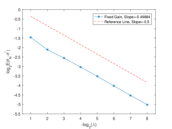
Figure 1: Rate of Convergence of Fixed Gain Algorithm for AR($1$) Process

5.2 Quantile estimation for MA($\infty$) processes

Let us now consider the case when $X_{t}$, $t\in\mathbb{N}$ is an MA($\infty$) process which is non-Markovian. It is given by

$$X_{t}=\sum_{j=0}^{\infty}\frac{1}{(j+1)^{\beta}}\varepsilon_{t-j}$$ (31)

where $\beta>1/2$ and $\varepsilon_{t}$, $t\in\mathbb{Z}$ are i.i.d sequence of standard normal variates. One can notice that the stationary distribution of MA($\infty$) process is given by

$$X_{t}\sim N\Big{(}0,\sum_{j=0}^{\infty}\frac{1}{(j+1)^{2\beta}}\Big{)}$$

for any $t\in\mathbb{N}$. As before, we are interested in the estimation of the quantile of the stationary distribution. In our numerical calculations, $\beta=3$ and the exact variance is $\pi^{6}/945$. For generating the path of the MA($\infty$) process, we write $X_{t}$ as

$$X_{t}=\sum_{j=0}^{t}\frac{1}{(j+1)^{\beta}}\varepsilon_{t-j}+\sum_{j=0}^{\infty}\frac{1}{(t+2+j)^{\beta}}\varepsilon_{-j-1}$$

and notice that

$$Y_{t}:=\sum_{j=0}^{\infty}\frac{1}{(t+2+j)^{\beta}}\varepsilon_{-j-1}\sim N\Big{(}0,\sum_{j=0}^{\infty}\frac{1}{(t+2+j)^{2\beta}}\Big{)}$$

for any $t\in\mathbb{N}$. Also, a reasonable approximation of the variance of $Y_{t}$ can be

$$\mathrm{var}(Y_{t})\approx\sum_{j=0}^{12}\frac{1}{(t+2+j)^{2\beta}}$$

which is within an interval of length $10^{-7}$ around the true value. With this set-up, the stochastic approximation method (29) with updating function (30) is implemented for the quantile estimation of the stationary distribution of MA($\infty$) process with $\theta_{0}=2.0$ and $\theta^{*}=1.976950$ ($0.975$-th quantile). Figure 2 indicates that the rate of convergence of the fixed gain algorithm is $0.5$, which is consistent with the theoretical findings. The Monte Carlo estimate is based on $10^{5}$ samples. Figure 2 is based on $I=10^{5}$ iterations.

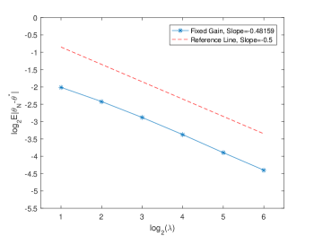
Figure 2: Rate of Convergence of Fixed Gain Algorithm for MA($\infty$) Process

5.3 Kohonen algorithm

In this section, we demonstrate the rate of convergence of the Kohonen algorithm for optimally quantizing a one-dimensional random variable $X$. We refer to [1, 9] for discussions. We fix the number of cells $N\geq 1$ in advance. Let $\theta:=(\theta^{1},\ldots,\theta^{N})\in\mathbb{R}^{N}$ and define Voronoi cells as

$$\mathcal{V}^{i}(\theta):=\{x\in\mathbb{R}:|x-\theta^{i}|=\min_{j\in\{1,\ldots,N\}}|x-\theta^{j}|\}$$

for $i=1,\ldots,N$. Values of $X$ in a cell $i$ will be quantized to $\theta^{i}$. The zero-neighbourhood fixed gain Kohonen algorithm is aimed at minimizing, in $\theta$, the quantity

$$\sum_{i+1}^{N}E\left[|X-\theta^{i}|^{2}1_{\mathcal{V}^{i}(\theta)}(X)\right].$$

Differentiating (formally) this formula suggests the recursive procedure

$$\theta_{t+1}^{i}=\theta_{t}^{i}+\lambda\mathbf{1}_{\mathcal{V}^{i}(\theta)}(Y_{t})(Y_{t}-\theta^{i}_{t})$$ (32)

for every $i=1,\ldots,N$ where $t\in\mathbb{N}$ and the process $Y$ has a stationary distribution equal to the law of $X$. The algorithm approximates the $\mathbb{R}$-valued random variable $X$ by $\theta^{i}$ if its values lie in the cell $\mathcal{V}^{i}(\theta)$, for every $i=1,\ldots,N$.

In Figure 3, we demonstrate the rate of convergence of the zero-neighbourhood Kohonen algorithm with zero-neighbours when the signal $Y_{t}$s are i.i.d. observations from uniform distribution on $[0,1]$, which is a well-understood case, see e.g. [1]. We take $N=2$, $\theta:=(\theta_{1},\theta_{2})$, $\mathcal{V}^{1}(\theta)=(0,(\theta^{1}+\theta^{2})/2]$ and $\mathcal{V}^{2}(\theta)=[(\theta_{1}+\theta_{2})/2,1)$. Hence, the optimal value of $\theta$ is $\theta^{1*}=1/4$ and $\theta^{2*}=3/4$. The number of iterations is $10^{8}$ and the number of sample paths is $10^{3}$. Furthermore, the initial values of $\theta$s are $\theta^{1}_{0}=0.01$ and $\theta^{2}_{0}=0.02$. As illustrated, the rate of convergence is close to $0.5$ which is consistent with the theoretical findings.

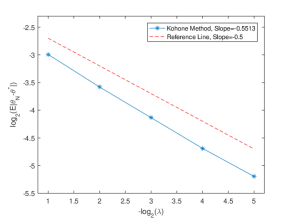
Figure 3: Rate of Convergence of Kohonen Algorithm for i.i.d. $U(0,1)$.

Now, to have a non-Markovian example, consider a moving average process with lag $10$, i.e.

$$X_{t}=\sum_{j=0}^{10}\frac{1}{(j+1)^{\beta}}\varepsilon_{t-j},\ t\in\mathbb{N},$$

where $\varepsilon_{t}$, $t\in\mathbb{Z}$ are independent standard Gaussian random variables, denote it by MA($10$). Clearly,

$$X_{t}\sim\mathcal{N}\Big{(}0,\sum_{j=0}^{10}\frac{1}{(j+1)^{2\beta}}\Big{)}$$

for any $t\geq 0$. Take $\beta:=3$ and notice that MA($10$) is a good approximation of MA($\infty$) process (31) because the contributions from other terms are negligible due to low variance. We take $N=2$ and implement the Kohonen algorithm (32) to sample two elements $\theta:=(\theta^{1},\theta^{2})$ from the stationary distribution of the process $Y$ defined by $Y_{t}:=\tan^{-1}(X_{t})$ for any $t\geq 0$. As the support of the stationary distribution of the process $Y$ is $(-\pi/2,\pi/2)$, the Voronoi cells are $\mathcal{V}^{1}(\theta):=(-\pi/2,(\theta^{1}+\theta^{2})/2]$ and $\mathcal{V}^{2}(\theta):=[(\theta^{1}+\theta_{2})/2,\pi/2)$. The true values $\theta^{*}:=(\theta^{1*},\theta^{2*})$ are the solution of the following system of two non-linear equations:

$$\theta^{1*}\Phi\Big{(}\frac{1}{\sigma}\tan\big{(}\frac{\theta^{1*}+\theta^{2*}}{2}\big{)}\Big{)}=E\Big{(}\tan^{-1}(\sigma Z)\mathbf{1}_{(-\infty,\frac{1}{\sigma}\tan(\frac{\theta^{1*}+\theta^{2*}}{2})]}(Z)\Big{)}$$

$$\theta^{2*}\Big{[}1-\Phi\Big{(}\frac{1}{\sigma}\tan\big{(}\frac{\theta^{1*}+\theta^{2*}}{2}\big{)}\Big{)}\Big{]}=E\Big{(}\tan^{-1}(\sigma Z)\mathbf{1}_{[\frac{1}{\sigma}\tan(\frac{\theta^{1*}+\theta^{2*}}{2}),\infty)}(Z)\Big{)}$$

where $\sigma^{2}:=\mathrm{var}(X_{t})$, $Z$ denotes the standard normal variate and $\Phi$ its distribution function.

Figure 4 is based on $10^{8}$ iterations and $3000$ paths (for Monte Carlo simulations). The initial values are $\theta_{0}^{1}=-\pi/4$ and $\theta_{0}^{2}=\pi/4$. Since $\theta^{*}$ is not known the output of the Kohonen algorithm (32) with $\lambda=2^{-9}$ is taken as $\theta^{*}$. Again, our numerical experiments are consistent with the theoretical rate $\lambda^{1/2}$ found in Theorem 3.6 above.

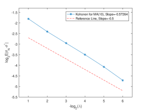
Figure 4: Rate of Convergence of Kohonen Algorithm for MA($10$).

6 Appendix

Here we gather the proofs for Sections 2 and 3 as well as for Theorem 4.19. First we present a slight extension of Lemma 2.1 of [12] which is used multiple times.

Lemma 6.1.

Let $\mathcal{G},\mathcal{H}\subset\mathcal{F}$ be sigma-algebras. Let $X,Y$ be random variables in $L^{p}$ such that $Y$ is measurable with respect to $\mathcal{H}\vee\mathcal{G}$. Then for any $p\geq 1$,

$$E^{1/p}\left[|X-E[X|\mathcal{H}\vee\mathcal{G}]|^{p}\big{|}\mathcal{G}\right]\leq 2E^{1/p}\left[|X-Y|^{p}\big{|}\mathcal{G}\right].$$

If $Y$ is $\mathcal{H}$-measurable then

$$\|X-E[X|\mathcal{H}]\|_{p}\leq 2\|X-Y\|_{p}.$$ (33)

Proof.

Since $Y$ is $\mathcal{H}\vee\mathcal{G}$-measurable,

$$E\left[|X-E\left[X|\mathcal{H}\vee\mathcal{G}\right]|^{p}\big{|}\mathcal{G}\right] \leq$$

$$2^{p-1}E\left[|X-Y|^{p}\big{|}\mathcal{G}\right]+2^{p-1}E\left[|Y-E\left[X|\mathcal{H}\vee\mathcal{G}\right]|^{p}\big{|}\mathcal{G}\right] \leq$$

$$2^{p-1}E\left[|X-Y|^{p}\big{|}\mathcal{G}\right]+2^{p-1}E\left[E\left[|Y-X|\big{|}\mathcal{H}\vee\mathcal{G}\right]^{p}\big{|}\mathcal{G}\right] \leq$$

$$2^{p-1}E\left[|X-Y|^{p}\big{|}\mathcal{G}\right]+2^{p-1}E\left[E\left[|Y-X|^{p}\big{|}\mathcal{H}\vee\mathcal{G}\right]\big{|}\mathcal{G}\right] \leq$$

$$2^{p}E\left[|Y-X|^{p}\big{|}\mathcal{G}\right],$$

by Jensen’s inequality. Now (33) follows by taking $\mathcal{G}$ to be the trivial sigma-algebra. ∎

We now note what happens to products of two random fields.

Lemma 6.2.

Let $X_{t}(\theta)$ be ULM-$rp$ and $Y_{t}(\theta)$ ULM-$rq$ where $r\geq 1$, $p>1$, $1/p+1/q=1$. Then $X_{t}(\theta)Y_{t}(\theta)$ is ULM-$r$.

Proof.

We drop $\theta$ in the notation. It is clear from Hölder’s inequality that

$$M_{r}(XY)\leq M_{rp}(X)M_{rq}(Y),$$

so $X_{t}Y_{t}$ is bounded in $L^{r}$. Using Lemma 6.1, let us estimate, for $t,m\geq 1$,

$$\|X_{t}Y_{t}-E[X_{t}Y_{t}|\mathcal{F}_{t-m}^{+}]\|_{r} \leq$$

$$2\|X_{t}Y_{t}-E[X_{t}|\mathcal{F}_{t-m}^{+}]E[Y_{t}|\mathcal{F}_{t-m}^{+}]\|_{r} \leq$$

$$2\|X_{t}Y_{t}-X_{t}E[Y_{t}|\mathcal{F}_{t-m}^{+}]\|_{r}+2\|X_{t}E[Y_{t}|\mathcal{F}_{t-m}^{+}]-E[X_{t}|\mathcal{F}_{t-m}^{+}]E[X_{t}|\mathcal{F}_{t-m}^{+}]\|_{r} \leq$$

$$2\|X_{t}\|_{rp}\|Y_{t}-E[Y_{t}|\mathcal{F}_{t-m}^{+}]\|_{rq}+2\|X_{t}-E[X_{t}|\mathcal{F}_{t-m}^{+}]\|_{rp}\|E[Y_{t}|\mathcal{F}_{t-m}^{+}]\|_{rq} \leq$$

$$2\|X_{t}\|_{rp}\|Y_{t}-E[Y_{t}|\mathcal{F}_{t-m}^{+}]\|_{rq}+2\|X_{t}-E[X_{t}|\mathcal{F}_{t-m}^{+}]\|_{rp}\|Y_{t}\|_{rq},$$

by Hölder’s and Jensen’s inequalities. This shows the $L$-mixing property of order $r$, noting the assumptions on $X_{t}$, $Y_{t}$. ∎

Lemma 6.3.

Let $D$ be bounded. Fix $n\in\mathbb{N}$ and let $\psi_{t}$, $t\geq n$ be a sequence of $D$-valued, $\mathcal{F}_{n}$-measurable random variables. Let $X_{t}(\theta)$, $\theta\in D$, $t\in\mathbb{N}$ be UCLM-$(p,1)$ for some $p>1$, satisfying the CLC property and define the process $Y_{t}:=X_{t}(\psi_{t})$, $t\geq n$. Then

$$M_{p}^{n}(Y)\leq M_{p}^{n}(X),\quad\Gamma_{p}^{n}(Y)\leq\Gamma_{p}^{n}(X)\mbox{ a.s.}$$

Proof.

If the $\psi_{t}$ are $\mathcal{F}_{n}$-measurable step functions then this follows easily from the definitions. For general $\psi_{t}$, one can take $\mathcal{F}_{n}$-measurable step function approximations $\psi^{k}_{t}$, $k\in\mathbb{N}$ of the $\psi_{t}$ (in the almost sure sense). The CLC property implies that $X_{t}(\psi^{k}_{t})$ tends to $X_{t}(\psi_{t})$ in probability as $k\to\infty$. By Fatou’s lemma, $M_{p}^{n}(Y(\psi^{k}_{\cdot}))\leq M_{p}^{n}(X)$, $k\in\mathbb{N}$ now implies $M_{p}^{n}(Y(\psi_{\cdot}))\leq M_{p}^{n}(X)$. The sequence $X_{t}(\psi^{k}_{t})$ is bounded in $L^{p}$. It follows that $E[X_{n+t}(\psi^{k}_{n+t})|\mathcal{F}_{n+t-\tau}^{+}\vee\mathcal{F}_{n}]$ tends to $E[X_{n+t}(\psi_{n+t})|\mathcal{F}_{n+t-\tau}^{+}\vee\mathcal{F}_{n}]$ in $L^{1}$, a fortiori, in probability. Hence, for each $\tau\geq 1$, $\gamma_{p}^{n}(Y(\psi_{\cdot}^{k}),\tau)\leq\gamma_{p}^{n}(X,\tau)$, $k\in\mathbb{N}$ implies $\gamma_{p}^{n}(Y(\psi_{\cdot}))\leq\gamma_{p}^{n}(X,\tau)$, by Fatou’s lemma. Consequently, $\Gamma_{p}^{n}(Y(\psi_{\cdot}))\leq\Gamma_{p}^{n}(X)$ a.s. ∎

Remark 6.4.

Fix $n\in\mathbb{N}$. Let $Y_{t}$ be a conditionally $L$-mixing process of order $(p,1)$ for some $p\geq 1$ and define $W_{t}:=Y_{t}-E[Y_{t}|\mathcal{F}_{n}]$, $t\geq n$. Then it is easy to check that $M^{n}_{p}(W)\leq 2M^{n}_{p}(Y)$ and $\Gamma_{p}^{n}(W)=\Gamma_{p}^{n}(Y)$.

Let us now enter the setting where for all $t\in\mathbb{N}$, $\mathcal{F}_{t}=\sigma(\varepsilon_{j},\ j\in\mathbb{N},\ j\leq t)$, $\mathcal{F}_{t}^{+}:=\sigma(\varepsilon_{j},\ j>t)$ for some i.i.d. sequence $\varepsilon_{j}$, $j\in\mathbb{Z}$ with values in some Polish space $\mathcal{X}$. Let $\mu$ be the law of $(\varepsilon_{0},\varepsilon_{-1},\ldots)$ on $\mathcal{X}^{-\mathbb{N}}$. For given $\mathbf{e}=(e_{0},e_{-1},\ldots)\in\mathcal{X}^{-\mathbb{N}}$ and $n\in\mathbb{N}$, we define the measure

$$P^{\mathbf{e},n}:=\left(\otimes_{i>n}\nu\right)\bigotimes\left(\otimes_{i\leq n}\delta_{e_{i-n}}\right),$$

where $\delta_{x}$ is the probability concentrated on the point $x\in\mathcal{X}$. The corresponding expectation will be denoted by $E^{\mathbf{e},n}[\cdot]$.

In this setting the concept of conditional $L$-mixing is easily related to “ordinary” $L$-mixing and we will be able to use results of [12] directly, see the proof of Theorem 2.5. For each $n\in\mathbb{Z}$, we denote by $Z_{n}$ the random variable $(\varepsilon_{n},\varepsilon_{n-1},\ldots)$ and by $\tilde{\mu}$ their law on $\mathcal{X}^{-\mathbb{N}}$ (which does not depend on $n$). Let $X_{t}$, $t\in\mathbb{N}$ be a stochastic process bounded in $L^{r}$ for some $r\geq 1$. We introduce the quantities

$$M^{\mathbf{e},n}_{r}(X) := \sup_{t\in\mathbb{N}}E^{\mathbf{e},n}[|X_{n+t}|^{r}]^{1/r},$$

$$\gamma^{\mathbf{e},n}_{r}(\tau,X) := \sup_{t\geq\tau}E^{\mathbf{e},n}[|X_{n+t}-E^{\mathbf{e},n}[X_{n+t}|\mathcal{F}_{n+t-\tau}^{+}]|^{r}]^{1/r},\ \tau\geq 1,$$

$$\Gamma^{\mathbf{e},n}_{r}(X) := \sum_{\tau=1}^{\infty}\gamma^{\mathbf{e},n}_{r}(\tau,X),$$

which are well-defined for $\tilde{\mu}$-almost every $\mathbf{e}$.

Proof of Theorem 2.5..

For any non-negative random variable $Y$ on $(\Omega,\mathcal{F},P)$,

$$E^{\mathbf{e},n}[Y]\Big{|}_{\mathbf{e}=Z_{n}} = E[Y|\mathcal{F}_{n}]\mbox{ a.s.}$$ (34)

This can easily be proved for indicators of the form $Y=1_{\{\varepsilon_{n+j}\in A_{j},\ -k\leq j\leq k\}}$ with some $k\in\mathbb{N}$ and with Borel sets $A_{j}\subset\mathcal{X}$ and then it extends to all non-negative measurable $Y$. It follows that

$$M^{n}_{r}(W)=M^{\mathbf{e},n}_{r}(W)|_{\mathbf{e}=Z_{n}}.$$ (35)

A similar argument also establishes

$$E^{\mathbf{e},n}[Y|\mathcal{F}_{n+t-\tau}^{+}]\Big{|}_{\mathbf{e}=Z_{n}} = E[Y|\mathcal{F}_{n+t-\tau}^{+}\vee\mathcal{F}_{n}]\mbox{ a.s.},$$ (36)

for all $t\geq 1$ and $1\leq\tau\leq t$ hence also

$$\gamma^{\mathbf{e},n}_{r}(\tau,X)|_{\mathbf{e}=Z_{n}}=\gamma^{n}_{r}(\tau,X)\mbox{ a.s.}$$ (37)

From the conditional $L$-mixing property of $W_{t}$, $t\in\mathbb{N}$ under $P$ (of order $(r,1)$) it follows that, for $\tilde{\mu}$-almost every $\mathbf{e}$, the process $W_{t+n}$, $t\in\mathbb{N}$ is $L$-mixing under $P^{\mathbf{e},n}$. Theorems 1.1 and 5.1 of [12] (applied under $P^{\mathbf{e},n}$) imply

$$E^{\mathbf{e},n}\left[\max_{n<t\leq m}\left|\sum_{s=n+1}^{t}b_{s}W_{s}\right|^{r}\right]^{1/r}\leq C_{r}\left(\sum_{s=n+1}^{m}b_{s}^{2}\right)^{1/2}\sqrt{{M}^{\mathbf{e},n}_{r}(W)\Gamma_{r}^{\mathbf{e},n}(W)},$$

for $\tilde{\mu}$-almost every $\mathbf{e}$. Now (34), (35) and (37) imply (9). ∎

Now we turn to the proofs of Section 3. We first recall Lemma 2.2 of [17], which states that the discrete flow defined by (38) below inherits the exponential stability property (12). Let $\mathbb{M}:=\{(m,n)\in\mathbb{N}:\ m\leq n\}$.

Lemma 6.5.

Let Assumptions 3.2 and 3.3 be in force. For each $0\leq m\leq n$ and $\xi\in D_{\xi}$, define $z:\mathbb{M}\times D\to D$ by the recursion

$$z(m,m,\xi):=\xi,\quad z(n+1,m,\xi):=z(n,m,\xi)+\lambda G(z(n,m,\xi)).$$ (38)

If $d$ is large enough and $\lambda$ is small enough then this makes sense and $z(n,m,\xi)\in D_{\theta}$ for all $n\geq m$. Furthermore, for each $\alpha^{\prime}<\alpha$ (see Assumption 3.3) there is $C(\alpha^{\prime})>0$ such that

$$\left|\frac{\partial}{\partial\xi}z(n,m,\xi)\right|\leq C(\alpha^{\prime})e^{-\lambda\alpha^{\prime}(n-m)}.$$ (39)

$\Box$

Remark 6.6.

Actually, the same arguments also imply that the recursion (38) is well-defined for all $\xi\in D_{\theta}$, stays in $D$ and satisfies (39), provided that $d^{\prime}$ is large enough and $\lambda$ is sufficiently small.

For convenience’s sake, we recall a result from [11], which is also given as Lemma 4.2 of [17].

Lemma 6.7.

Let Assumptions 3.2 and 3.3 be satisfied. Let $y_{t}:=y(t,0,\xi)$, $t\geq 0$. Let $x_{t}$, $t\geq 0$ be a continuous, piecewise continuously differentiable curve such that $x_{0}=\xi$. Then for $t\geq 0$,

$$x_{t}-y_{t}=\int_{0}^{t}{\frac{\partial}{\partial\xi}y(t,w,x_{w})(\dot{x}_{w}-G(x_{w}))dw}.$$ (40)

Proof.

For $0\leq w\leq t$, let $z_{w}=y(t,w,x_{w})$. The LHS of (40) can be written as

$$z_{t}-z_{0}=\int_{0}^{t}{\dot{z}_{w}dw}=\int_{0}^{t}{\left(\frac{\partial}{\partial w}y(t,w,x_{w})+\frac{\partial}{\partial\xi}y(t,w,x_{w})\dot{x}_{w}\right)dw}.$$

From Theorem 3.1 on page 96 of [23] we obtain that, for all $x\in\mathbb{R}$,

$$\frac{\partial}{\partial w}y(t,w,x)+\frac{\partial}{\partial\xi}y(t,w,x)G(x)=0,$$

and hence the proof is complete. ∎

Let $\xi\in D_{\theta}$ and define $\tilde{z}_{n}:=z(n,0,\xi)$, $n\in\mathbb{N}$. The next lemma summarizes some arguments of [17] in the present setting, for the sake of a self-contained presentation.

Lemma 6.8.

Let Assumptions 3.2 and 3.3 be satisfied. Let $y_{t}:=y(t,0,\xi)$ for some $\xi\in D_{\xi}$ and let $\theta_{n}$ be defined by (15). If $d,d^{\prime}$ are large enough then, for all $n\in\mathbb{N}$, we have $\theta_{n}\in D_{\theta}$ and also $\tilde{z}_{n}\in D$.

Proof.

We denote by $\theta_{t}$ the piecewise linear extension of $\theta_{n}$, i.e. for $t\in(n,n+1)$, we set $\theta_{t}=(1-(t-n))\theta_{n}+(t-n)\theta_{n+1}.$ For $w\in(n,n+1)$, it is easy to see that $\dot{\theta}_{w}=\theta_{n+1}-\theta_{n}=\lambda H(\theta_{[w]},X_{[w]+1})$ where $[w]$ denotes the integer part of $w$. Thus, Lemma 6.7 implies that as long as $\theta_{w}\in D_{\theta}$ for all $0\leq w\leq t$,

$$\theta_{t}-y_{t}=\int_{0}^{t}{\frac{\partial}{\partial\xi}y(t,w,\theta_{w})\lambda\left(H(\theta_{[w]},X_{[w]+1})-G(\theta_{w})\right)dw}.$$

Since $|H|$ and $|G|$ are bounded by a constant, say, $C^{\dagger}$, (12) implies that

$$|\theta_{t}-y_{t}|\leq\int_{0}^{t}{C^{*}e^{-\lambda\alpha(t-w)}\lambda 2C^{\dagger}dw}\leq 2C^{*}C^{\dagger}\alpha^{-1}.$$

It is known that $y_{t}\in D_{y}$ whenever $y_{0}\in D_{\xi}$. Now, if $d>2C^{*}C^{\dagger}\alpha^{-1}$ then $|\theta_{t}-y_{t}|$ will be smaller than the distance between $D_{y}$ and $D_{\theta}^{c}$, where $D_{\theta}^{c}$ denotes the complement of $D_{\theta}$, hence $\theta_{t}$ will stay in $D_{\theta}$ for ever.

The proof for $\tilde{z}_{n}\in D$ is similar. The piecewise linear extension of $\tilde{z}_{n}$ is denoted by $\tilde{z}_{t}$, $t\geq 0$. By computations as before,

$$\tilde{z}_{t}-y_{t}=\int_{0}^{t}{\frac{\partial}{\partial\xi}y(t,w,\tilde{z}_{w})\lambda\left(G(\tilde{z}_{[w]})-G(\tilde{z}_{w})\right)dw}.$$

Denoting by $K^{*}$ (resp. $L^{*}$) a bound for $|G|$ (resp. a Lipschitz-constant for $G$), we obtain

$$|G(\tilde{z}_{[w]})-G(\tilde{z}_{w})|\leq L^{*}|\tilde{z}_{[w]}-\tilde{z}_{w}|\leq L^{*}\lambda G(\tilde{z}_{[w]})\leq\lambda L^{*}K^{*},$$

hence

$$|\tilde{z}_{t}-y_{t}|\leq\int_{0}^{t}{C^{*}e^{-\lambda\alpha(t-w)}\lambda^{2}L^{*}K^{*}dw}\leq C^{*}\alpha^{-1}\lambda L^{*}K^{*}.$$

It follows that if $d^{\prime}>C^{*}\alpha^{-1}\lambda L^{*}K^{*}$ then $\tilde{z}_{t}\in D$, for all $t$. ∎

Remark 6.9.

Note that our estimates for $d$, $d^{\prime}$ in the above proof are somewhat different: by choosing $\lambda$ small enough we can make $d^{\prime}$ as small as we wish whereas we do not have this option for $d$. This is in contrast with [17], where $d$ can also be made arbitrarily small by choosing $\lambda$ small. This difference comes from the fact that in [17] Lipschitz-continuity of $\theta\to H(\theta,\cdot)$ is assumed, unlike in the present setting.

Proof of Theorem 3.6..

We follow the main lines of the arguments in [14, 17]. However, details deviate significantly as our present assumptions are different from those of the cited papers.

Lemma 6.8 above will guarantee that $\theta_{t}$ and $z_{t},\overline{z}_{t}$ (see below) are well-defined. Clearly, $z_{t}=z(t,0,\theta_{0})$. Set $T=[1/(\lambda\alpha^{\prime})]$, where $0<\alpha^{\prime}<\alpha$ is as in Lemma 6.5 and $[x]$ denotes the integer part of $x\in\mathbb{R}$. For each $n\in\mathbb{N}$, we set $\overline{z}_{nT}:=\theta_{nT}$ and define recursively

$$\overline{z}_{t}: =\overline{z}_{t-1}+\lambda G(\overline{z}_{t-1}),\qquad nT<t<(n+1)T.$$

In other words, $\overline{z}_{t}=z(t,nT,\theta_{nT})$. By the triangle inequality, we obtain, for any $t\in\mathbb{N}$,

$$|\theta_{t}-z_{t}|\leq|\theta_{t}-\overline{z}_{t}|+|\overline{z}_{t}-z_{t}|.$$ (41)

Estimation for $|\theta_{t}-\overline{z}_{t}|$. Fix $n$ and let $nT<t<(n+1)T$.

$$|\theta_{t}-\overline{z}_{t}|=\lambda\left|\sum_{k=nT}^{t-1}[H(\theta_{k},X_{k+1})-G(\overline{z}_{k})]\right| \leq$$

$$\lambda\sum_{k=nT}^{t-1}\left|H(\theta_{k},X_{k+1})-H(\overline{z}_{k},X_{k+1})\right| +$$

$$\lambda\left|\sum_{k=nT}^{t-1}\left(H(\overline{z}_{k},X_{k+1})-E[H(\overline{z}_{k},X_{k+1})|\mathcal{F}_{nT}]\right)\right| +$$

$$\lambda\sum_{k=nT}^{t-1}\left|E[H(\overline{z}_{k},X_{k+1})|\mathcal{F}_{nT}]-G(\overline{z}_{k})\right| =: \lambda(S_{1}+S_{2}+S_{3}).$$

It is clear that

$$ES_{3} \leq E\left[\sup_{\vartheta\in D}\sum_{k=nT}^{\infty}\left|E[H(\vartheta,X_{k+1})|\mathcal{F}_{nT}]-G(\vartheta)\right|\right]<C^{\prime},$$

for some $C^{\prime}<\infty$, by Assumption 3.4.

Turning our attention to $S_{1}$, the CLC property implies

$$ES_{1}=E[E[S_{1}|\mathcal{F}_{nT}]]\leq\sum_{k=nT}^{t-1}KE|\theta_{k}-\overline{z}_{k}|.$$

On each interval $nT\leq t<(n+1)T$, we now estimate $S_{2}$ as follows,

$$S_{2}\leq\sup_{nT<t\leq(n+1)T}\left|\sum_{k=nT}^{t-1}\left(H(\overline{z}_{k},X_{k+1})-E[H(\overline{z}_{k},X_{k+1})|\mathcal{F}_{nT}]\right)\right|.$$

Note the UCLM-$(r,1)$ property of $H(\cdot,\cdot)$ as well as Lemma 6.3 and Remark 6.4. Apply Theorem 2.5 for $nT$ instead of $n$ and with the choice $b_{t}\equiv 1$ and

$$W_{t}:=H(\overline{z}_{t},X_{t+1})-E[H(\overline{z}_{t},X_{t+1})|\mathcal{F}_{nT}],\ nT<t\leq(n+1)T,\ W_{t}:=0,\ 0\leq t\leq nT,$$

note that $E[W_{t}|\mathcal{F}_{nT}]=0$ for all $t$. We get

$$ES_{2}=E[E[S_{2}|\mathcal{F}_{nT}]]\leq E[E^{1/r}[S_{2}^{r}|\mathcal{F}_{nT}]] \leq$$

$$C_{r}T^{1/2}E\left[\sqrt{M^{nT}_{r}(W)\Gamma^{nT}_{r}(W)}\right]\leq C_{r}T^{1/2}\sqrt{EM^{nT}_{r}(W)E\Gamma^{nT}_{r}(W)} \leq$$

$$C^{\prime\prime}T^{1/2}$$

with some $C^{\prime\prime}<\infty$, independent of $n$, by the UCLM-$(r,1)$ property of $W$.

Putting together our estimates so far, we obtain for $nT\leq t<(n+1)T$,

$$E|\theta_{t}-\overline{z}_{t}|\leq\lambda\left(\sum_{k=nT}^{t-1}KE|\theta_{k}-\overline{z}_{k}|+C^{\prime\prime}T^{1/2}+C^{\prime}\right).$$

Recall that $E|\theta_{t}-\overline{z}_{t}|$ is finite by boundedness of $D$. The discrete Gronwall lemma yields the following estimate, independent of $n$:

$$E|\theta_{t}-\overline{z}_{t}|\leq\lambda(C^{\prime\prime}T^{1/2}+C^{\prime})(1+\lambda K)^{T}.$$ (42)

Note that

$$(1+\lambda K)^{T}\leq e^{\lambda KT}\leq e^{K/\alpha^{\prime}}.$$

Estimation for $|\overline{z}_{t}-z_{t}|$. Noting $z_{0}=\theta_{0}$ and using the fundamental theorem of calculus, we estimate for $nT\leq t<(n+1)T$, using telescoping sums,

$$|\bar{z}_{t}-z_{t}|$$

$$\leq \sum_{k=1}^{n}|z(t,kT,\theta_{kT})-z(t,(k-1)T,\theta_{(k-1)T})|$$

$$= \sum_{k=1}^{n}|z(t,kT,\theta_{kT})-z(t,kT,z(kT,(k-1)T,\theta_{(k-1)T}))|$$

$$= \sum_{k=1}^{n}\int_{0}^{1}\left|\frac{\partial}{\partial\xi}z(t,kT,s\theta_{kT}+(1-s)z(kT,(k-1)T,\theta_{(k-1)T}))\right|ds$$

$$\times |\theta_{kT}-z(kT,(k-1)T,\theta_{(k-1)T})|$$

$$\leq C(\alpha^{\prime})\sum_{k=1}^{n}e^{-\lambda\alpha^{\prime}(t-kT)}\left(|\theta_{kT-1}-\bar{z}_{kT-1}|+\lambda|H(\theta_{kT-1},X_{kT})-G(\overline{z}_{kT-1})|\right).$$

Notice that there is $\tilde{C}>0$, independent of $n,t$ such that

$$\sum_{k=1}^{n}e^{-\lambda\alpha^{\prime}(t-kT)}\leq\tilde{C}.$$

Therefore, the fact that $H$, $G$, $D$ are bounded, imply

$$E|\overline{z}_{t}-z_{t}| \leq c\sum_{k=1}^{n}e^{-\lambda\alpha^{\prime}(t-kT)}E|\theta_{kT-1}-\bar{z}_{kT-1}|+c\sum_{k=1}^{n}e^{-\lambda\alpha^{\prime}(t-kT)}\lambda$$ (43)

$$\leq c^{\prime}\lambda^{1/2},$$

with some $c,c^{\prime}>0$, by (42) and by the choice of $T$. Finally, putting together our estimations (42), (43) and using (41), for $\lambda$ small enough, we obtain

$$E|\theta_{t}-z_{t}|\leq C\lambda^{1/2},$$

with some $C>0$, which completes the proof. ∎

Proof of Corollary 3.7..

Recall $\alpha^{\prime}$ from Lemma 6.5. The fundamental theorem of calculus yields

$$|z_{t}-\theta^{*}| \leq|z_{0}-\theta^{*}|\int_{0}^{1}\left|\frac{\partial}{\partial\xi}z(t,0,sz_{0}+(1-s)\theta^{*})\right|ds$$

$$\leq C(\alpha^{\prime})e^{-\lambda\alpha^{\prime}t}|z_{0}-\theta^{*}|,$$

and this is $\leq\lambda^{1/2}$ for $t\geq t_{0}(\lambda)$ if $t_{0}(\lambda)=C^{\circ}\ln(1/\lambda)/\lambda$ for some $C^{\circ}$. Since

$$|\theta_{t}-\theta^{*}|\leq|\theta_{t}-z_{t}|+|z_{t}-\theta^{*}|,$$

the statement follows. ∎

Proof of Theorem 4.19..

Let us work conditionally on the event $\mathcal{E}_{0}=\eta\in\mathbb{R}^{\mathbb{Z}}$ where

$$\mathcal{E}_{l}=(\varepsilon^{1}_{i+l})_{i\in\mathbb{Z}},$$

until further notice.

The CLC property and Assumption 3.2 are trivial. Define $\mathcal{F}_{n}:=\sigma(\varepsilon^{2}_{j};j\leq n)$ and $\mathcal{F}^{+}_{n}:=\sigma(\varepsilon^{2}_{j};j>n)$.

We now prove that $H(\theta,X_{t})$ is UCLM-$(r,1)$ with respect to the given $(\mathcal{F}_{n},\mathcal{F}^{+}_{n})$. Boundedness of $H$ implies that $M^{n}_{r}(X)$, $n\in\mathbb{N}$ is uniformly bounded.

Fix $1\leq m\leq t$. Define recursively

$$\xi_{t-m}:=x,\quad\xi_{l+1}:=F(\mathcal{E}_{l+1},\varepsilon_{l+1}^{2},\xi_{l}),\ l\geq t-m.$$

Set $X_{t,m}^{+}:=\xi_{t}$. By construction, $X_{t,m}^{+}$ is $\mathcal{F}_{t-m}^{+}$-measurable and

$$|H(\theta,X_{t,m}^{+})-H(\theta,X_{t})|\leq L\rho^{m}|x-X_{t-m}|,$$

where $L$ is a Lipschitz-constant for $x\to H(\theta,x)$. So we can further estimate

$$E\left[|x-X_{t-m}|^{r}\big{|}\mathcal{F}_{0}\right]^{1/r}\leq\sum_{j=1}^{\infty}E\left[|\tilde{X}^{t-m}_{j}-\tilde{X}^{t-m}_{j-1}|^{r}\big{|}\mathcal{F}_{0}\right]^{1/r} \leq$$

$$\sum_{j=1}^{\infty}\rho^{j-1}E\left[|x-F(\mathbf{f}_{t-m-j+1},\varepsilon_{t-m-j+1}^{2},x)|^{r}\big{|}\mathcal{F}_{0}\right]^{1/r} \leq$$

$$C\sum_{j=1}^{t-m}\rho^{j-1}\||\varepsilon_{t-m-j+1}^{2}|+1\|_{r}+C\sum_{j=t-m+1}^{\infty}\rho^{j-1}[|\varepsilon_{t-m-j+1}^{2}|+1] \leq$$

$$C\||\varepsilon_{0}^{2}|+1\|_{r}\sum_{j=1}^{\infty}\rho^{j-1}+C\sum_{k=0}^{\infty}\rho^{t-m+k}[|\varepsilon_{-k}^{2}|+1] \leq$$

$$C\||\varepsilon_{0}^{2}|+1\|_{r}\sum_{j=1}^{\infty}\rho^{j-1}+C\sum_{k=0}^{\infty}\rho^{k}[|\varepsilon_{-k}^{2}|+1],$$

using Assumption 4.17, the independence of $\varepsilon_{j}^{2}$, $j\geq 1$ from $\mathcal{F}_{0}$ and the $\mathcal{F}_{0}$-measurability of $\varepsilon^{2}_{j}$, $j\leq 0$. Note that this last estimate is independent of $t$. We can carry out analogous estimates with $\mathcal{F}_{n}$ instead of $\mathcal{F}_{0}$ and these imply, via Lemma 6.1,

$$\gamma_{r}^{n}(m,X)\leq 2LC\rho^{m}\left[(\|\varepsilon_{0}^{2}\|_{r}+1)\sum_{j=1}^{\infty}\rho^{j-1}+\sum_{k=0}^{\infty}\rho^{k}[|\varepsilon_{n-k}^{2}|+1]\right],$$

for each $n\in\mathbb{N}$, which implies that the sequence $\Gamma^{n}_{r}(X)$ is bounded in $L^{1}$, showing the UCLM-$(r,1)$ property for $H(\theta,X_{t})$.

Since $X_{t-m}^{+}$ is $\mathcal{F}_{t-m}^{+}$-measurable, the above estimates also show that $H(\theta,X_{t})$ is (unconditionally) $L$-mixing of order $(r,1)$, hence Remark 3.5 implies Assumption 3.4. As the estimates are uniform in $\eta\in\mathbb{R}^{\mathbb{Z}}$, the argument of Theorem 3.6 can be applied. ∎

7 Conclusion

There is a large number of natural ramifications of our results that could be pursued: the estimation of higher order moments of the tracking error using the property UCLM-$(r,p)$ for $p>1$; accommodating multiple roots for equation (13); proving the convergence of the decreasing gain version of (1); considering the convergence of concrete procedures. We leave these for later work in order to convey a clear message, highlighting the novel techniques we have introduced.

Acknowledgments. We thank two anonymous referees for several insightful comments that led to substantial improvements. The major part of this work was done while the second author was working as a Whittaker Research Fellow in Stochastic Analysis in the School of Mathematics, University of Edinburgh, United Kingdom. We have made use of the resources provided by the Edinburgh Compute and Data Facility (ECDF), see

$$\mathtt{http://www.ecdf.ed.ac.uk/}$$

This work was supported by The Alan Turing Institute under the EPSRC grant EP/N510129/1, in the framework of a “small research group”, during the summer of 2016. Huy N. Chau and Miklós Rásonyi were also supported by the “Lendület” Grant LP2015-6 of the Hungarian Academy of Sciences and by the NKFIH (National Research, Development and Innovation Office, Hungary) grant KH 126505. Sotirios Sabanis gratefully acknowledges the support of the Royal Society through the IE150128 grant. We thank László Gerencsér for helpful discussions and dedicate this paper to him.

References

- [1] M. Benaim, J.-C. Fort and G. Pagès. Convergence of the one-dimensional Kohonen algorithm. Advances in Applied Probability, 30:850-869, 1998.
- [2] R. Bhattacharya and E. C. Waymire. An approach to the existence of unique invariant probabilities for Markov processes. In: Limit theorems in probability and statistics, János Bolyai Math. Soc., I, 181–200, 2002.
- [3] J. A. Bucklew, T. G. Kurtz and W. A. Sethares. Weak convergence and local stability properties of fixed step size recursive algorithms. IEEE Trans. Inform. Theory, 39:966–978, 1993.
- [4] F. Comte and É. Renault. Long memory in continuous-time stochastic volatility models. Mathematical Finance, 8:291–323, 1998.
- [5] P. Diaconis and D. Freedman. Iterated random functions. SIAM Review, 41:45–76, 1999.
- [6] S. N. Ethier and T. G. Kurtz. Markov processes. Characterization and convergence. Wiley, New York, 1986.
- [7] E. Eweda. Analysis and design of a signed regressor LMS algorithm for stationary and nonstationary adaptive filtering with correlated Gaussian data. IEEE Transactions on Circuits and Systems, 37: 1367-1374, 1990.
- [8] E. Eweda. Convergence analysis of an adaptive filter equipped with the sign-sign algorithm. IEEE Transactions on Automatic Control, 40:1807-1811, 1995.
- [9] G. Fort, É. Moulines, A. Schreck and M. Vihola. Convergence of Markovian stochastic approximation with discontinuous dynamics. SIAM Journal on Control and Optimization, 54:866–893, 2016.
- [10] J. Gatheral, Th. Jaisson and M. Rosenbaum. Volatility is rough. Quantitative Finance, 18:933–949, 2018.
- [11] S. Geman. Some averaging and stability results for random differential equations. SIAM Journal on Applied Mathematics, 36:86–105, 1979.
- [12] L. Gerencsér. On a class of mixing processes. Stochastics, 26:165–191, 1989.
- [13] L. Gerencsér. estimation and nonparametric stochastic complexity. IEEE Trans. Inform. Theory, 38:1768–1778, 1992.
- [14] L. Gerencsér. On fixed gain recursive estimation processes. J. Mathematical Systems, Estimation and Control, 6:355–358, 1996. Retrieval code for full electronic manuscript: 56854
- [15] L. Gerencsér. Strong approximation of the recursive prediction error estimator of the parameters of an ARMA process. Systems Control Lett., 21:347–351, 1993.
- [16] L. Gerencsér. On Rissanen’s predictive stochastic complexity for stationary ARMA processes. J. Statist. Plann. Inference, 41:303–325, 1994.
- [17] L. Gerencsér. Stability of random iterative mappings. In: Modeling uncertainty. An examination of stochastic theory, methods, and applications. (ed. M. Dror, P. L’Écuyer, F. Szidarovszky), International Series in Operations Research and Management Science vol. 46, Kluwer Academic Publishers, 359–371, 2002.
- [18] L. Gerencsér. A representation theorem for the error of recursive estimators. SIAM J. Control Optim., 44:2123–2188, 2006.
- [19] L. Gerencsér. Rate of convergence of recursive estimators. SIAM J. Control Optim., 30:1200–1227, 1992.
- [20] L. Gerencsér, G. Molnár-Sáska, Gy. Michaletzky, G. Tusnády and Zs. Vágó. New methods for the statistical analysis of Hidden Markov models. In:Proceedings of the 41st IEEE Conference on Decision and Control, 2002, Las Vegas, USA 2272–2277, IEEE Press, New York, 2002.
- [21] L. Giraitis, H. L. Koul and D. Surgailis. Large sample inference for long memory processes. Imperial College Press, London, 2012.
- [22] M. Hairer and J. Mattingly. Yet another look at Harris’ ergodic theorem for Markov chains. In: Seminar on stochastic analysis, random fields and applications VI (eds. R. Dalang, M. Dozzi and F. Russo), Progress in Probability, vol. 63, 109–117, 2011.
- [23] Ph. Hartman. Ordinary differential equations. Classics in Applied Mathematics, 38, 2nd edition, SIAM, 2002.
- [24] O. Kallenberg. Foundations of modern probability. 2nd edition, Springer, 2002.
- [25] T. Kawata. Fourier analysis in probability theory. Academic Press, 1972.
- [26] R. Koenker and G. Bassett Jr. Regression quantiles. Econometrica, 46:33-50, 1978.
- [27] T. Kohonen. Analysis of a simple self-organising process. Biological Cybernetics, 44:135–140, 1982.
- [28] S. Laruelle and G. Pagès. Stochastic approximation with averaging innovation applied to finance. Monte Carlo Methods Appl. 18:1–51, 2012.
- [29] J.Neveu. Discrete-parameter martingales. North-Holland, 1975.
- [30] M. Rásonyi. On the statistical analysis of quantized Gaussian AR(1) processes. Int. J. of Adaptive Control and Signal Processing, 24:490–507, 2010.