Photo-Realistic Single Image Super-Resolution Using a Generative Adversarial Network
Abstract
Despite the breakthroughs in accuracy and speed of single image super-resolution using faster and deeper convolutional neural networks, one central problem remains largely unsolved: how do we recover the finer texture details when we super-resolve at large upscaling factors? The behavior of optimization-based super-resolution methods is principally driven by the choice of the objective function. Recent work has largely focused on minimizing the mean squared reconstruction error. The resulting estimates have high peak signal-to-noise ratios, but they are often lacking high-frequency details and are perceptually unsatisfying in the sense that they fail to match the fidelity expected at the higher resolution. In this paper, we present SRGAN, a generative adversarial network (GAN) for image super-resolution (SR). To our knowledge, it is the first framework capable of inferring photo-realistic natural images for upscaling factors. To achieve this, we propose a perceptual loss function which consists of an adversarial loss and a content loss. The adversarial loss pushes our solution to the natural image manifold using a discriminator network that is trained to differentiate between the super-resolved images and original photo-realistic images. In addition, we use a content loss motivated by perceptual similarity instead of similarity in pixel space. Our deep residual network is able to recover photo-realistic textures from heavily downsampled images on public benchmarks. An extensive mean-opinion-score (MOS) test shows hugely significant gains in perceptual quality using SRGAN. The MOS scores obtained with SRGAN are closer to those of the original high-resolution images than to those obtained with any state-of-the-art method.
1 Introduction
The highly challenging task of estimating a high-resolution (HR) image from its low-resolution (LR) counterpart is referred to as super-resolution (SR). SR received substantial attention from within the computer vision research community and has a wide range of applications [63, 71, 43].
| SRGAN (proposed) | original |
|---|---|
 |
 |
The ill-posed nature of the underdetermined SR problem is particularly pronounced for high upscaling factors, for which texture detail in the reconstructed SR images is typically absent.
| bicubic | SRResNet | SRGAN | original |
| (21.59dB/0.6423) | (23.53dB/0.7832) | (21.15dB/0.6868) | |
 |
 |
 |
 |
The optimization target of supervised SR algorithms is commonly the minimization of the mean squared error (MSE) between the recovered HR image and the ground truth. This is convenient as minimizing MSE also maximizes the peak signal-to-noise ratio (PSNR), which is a common measure used to evaluate and compare SR algorithms [61]. However, the ability of MSE (and PSNR) to capture perceptually relevant differences, such as high texture detail, is very limited as they are defined based on pixel-wise image differences [60, 58, 26]. This is illustrated in Figure 2, where highest PSNR does not necessarily reflect the perceptually better SR result. The perceptual difference between the super-resolved and original image means that the recovered image is not photo-realistic as defined by Ferwerda [16].
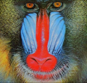
In this work we propose a super-resolution generative adversarial network (SRGAN) for which we employ a deep residual network (ResNet) with skip-connection and diverge from MSE as the sole optimization target. Different from previous works, we define a novel perceptual loss using high-level feature maps of the VGG network [49, 33, 5] combined with a discriminator that encourages solutions perceptually hard to distinguish from the HR reference images. An example photo-realistic image that was super-resolved with a upscaling factor is shown in Figure 1.
1.1 Related work
1.1.1 Image super-resolution
Recent overview articles on image SR include Nasrollahi and Moeslund [43] or Yang et al. [61]. Here we will focus on single image super-resolution (SISR) and will not further discuss approaches that recover HR images from multiple images [4, 15].
Prediction-based methods were among the first methods to tackle SISR. While these filtering approaches, e.g. linear, bicubic or Lanczos [14] filtering, can be very fast, they oversimplify the SISR problem and usually yield solutions with overly smooth textures. Methods that put particularly focus on edge-preservation have been proposed [1, 39].
More powerful approaches aim to establish a complex mapping between low- and high-resolution image information and usually rely on training data. Many methods that are based on example-pairs rely on LR training patches for which the corresponding HR counterparts are known. Early work was presented by Freeman et al. [18, 17]. Related approaches to the SR problem originate in compressed sensing [62, 12, 69]. In Glasner et al. [21] the authors exploit patch redundancies across scales within the image to drive the SR. This paradigm of self-similarity is also employed in Huang et al. [31], where self dictionaries are extended by further allowing for small transformations and shape variations. Gu et al. [25] proposed a convolutional sparse coding approach that improves consistency by processing the whole image rather than overlapping patches.
To reconstruct realistic texture detail while avoiding edge artifacts, Tai et al. [52] combine an edge-directed SR algorithm based on a gradient profile prior [50] with the benefits of learning-based detail synthesis. Zhang et al. [70] propose a multi-scale dictionary to capture redundancies of similar image patches at different scales. To super-resolve landmark images, Yue et al. [67] retrieve correlating HR images with similar content from the web and propose a structure-aware matching criterion for alignment.
Neighborhood embedding approaches upsample a LR image patch by finding similar LR training patches in a low dimensional manifold and combining their corresponding HR patches for reconstruction [54, 55]. In Kim and Kwon [35] the authors emphasize the tendency of neighborhood approaches to overfit and formulate a more general map of example pairs using kernel ridge regression. The regression problem can also be solved with Gaussian process regression [27], trees [46] or Random Forests [47]. In Dai et al. [6] a multitude of patch-specific regressors is learned and the most appropriate regressors selected during testing.
Recently convolutional neural network (CNN) based SR algorithms have shown excellent performance. In Wang et al. [59] the authors encode a sparse representation prior into their feed-forward network architecture based on the learned iterative shrinkage and thresholding algorithm (LISTA) [23]. Dong et al. [9, 10] used bicubic interpolation to upscale an input image and trained a three layer deep fully convolutional network end-to-end to achieve state-of-the-art SR performance. Subsequently, it was shown that enabling the network to learn the upscaling filters directly can further increase performance both in terms of accuracy and speed [11, 48, 57]. With their deeply-recursive convolutional network (DRCN), Kim et al. [34] presented a highly performant architecture that allows for long-range pixel dependencies while keeping the number of model parameters small. Of particular relevance for our paper are the works by Johnson et al. [33] and Bruna et al. [5], who rely on a loss function closer to perceptual similarity to recover visually more convincing HR images.
1.1.2 Design of convolutional neural networks
The state of the art for many computer vision problems is meanwhile set by specifically designed CNN architectures following the success of the work by Krizhevsky et al. [37].
It was shown that deeper network architectures can be difficult to train but have the potential to substantially increase the network’s accuracy as they allow modeling mappings of very high complexity [49, 51]. To efficiently train these deeper network architectures, batch-normalization [32] is often used to counteract the internal co-variate shift. Deeper network architectures have also been shown to increase performance for SISR, e.g. Kim et al. [34] formulate a recursive CNN and present state-of-the-art results. Another powerful design choice that eases the training of deep CNN s is the recently introduced concept of residual blocks [29] and skip-connections [30, 34]. Skip-connections relieve the network architecture of modeling the identity mapping that is trivial in nature, however, potentially non-trivial to represent with convolutional kernels.
In the context of SISR it was also shown that learning upscaling filters is beneficial in terms of accuracy and speed [11, 48, 57]. This is an improvement over Dong et al. [10] where bicubic interpolation is employed to upscale the LR observation before feeding the image to the CNN.
1.1.3 Loss functions
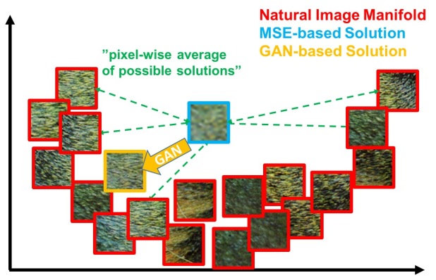
Pixel-wise loss functions such as MSE struggle to handle the uncertainty inherent in recovering lost high-frequency details such as texture: minimizing MSE encourages finding pixel-wise averages of plausible solutions which are typically overly-smooth and thus have poor perceptual quality [42, 33, 13, 5]. Reconstructions of varying perceptual quality are exemplified with corresponding PSNR in Figure 2. We illustrate the problem of minimizing MSE in Figure 3 where multiple potential solutions with high texture details are averaged to create a smooth reconstruction.
In Mathieu et al. [42] and Denton et al. [7] the authors tackled this problem by employing generative adversarial networks (GANs) [22] for the application of image generation. Yu and Porikli [66] augment pixel-wise MSE loss with a discriminator loss to train a network that super-resolves face images with large upscaling factors (). GANs were also used for unsupervised representation learning in Radford et al. [44]. The idea of using GANs to learn a mapping from one manifold to another is described by Li and Wand [38] for style transfer and Yeh et al. [64] for inpainting. Bruna et al. [5] minimize the squared error in the feature spaces of VGG19 [49] and scattering networks.
Dosovitskiy and Brox [13] use loss functions based on Euclidean distances computed in the feature space of neural networks in combination with adversarial training. It is shown that the proposed loss allows visually superior image generation and can be used to solve the ill-posed inverse problem of decoding nonlinear feature representations. Similar to this work, Johnson et al. [33] and Bruna et al. [5] propose the use of features extracted from a pre-trained VGG network instead of low-level pixel-wise error measures. Specifically the authors formulate a loss function based on the euclidean distance between feature maps extracted from the VGG19 [49] network. Perceptually more convincing results were obtained for both super-resolution and artistic style-transfer [19, 20]. Recently, Li and Wand [38] also investigated the effect of comparing and blending patches in pixel or VGG feature space.
1.2 Contribution
GANs provide a powerful framework for generating plausible-looking natural images with high perceptual quality. The GAN procedure encourages the reconstructions to move towards regions of the search space with high probability of containing photo-realistic images and thus closer to the natural image manifold as shown in Figure 3.
In this paper we describe the first very deep ResNet [29, 30] architecture using the concept of GANs to form a perceptual loss function for photo-realistic SISR. Our main contributions are:
-
•
We set a new state of the art for image SR with high upscaling factors () as measured by PSNR and structural similarity (SSIM) with our 16 blocks deep ResNet (SRResNet) optimized for MSE.
- •
-
•
We confirm with an extensive mean opinion score (MOS) test on images from three public benchmark datasets that SRGAN is the new state of the art, by a large margin, for the estimation of photo-realistic SR images with high upscaling factors ().
2 Method
 |
 |
In SISR the aim is to estimate a high-resolution, super-resolved image from a low-resolution input image . Here is the low-resolution version of its high-resolution counterpart . The high-resolution images are only available during training. In training, is obtained by applying a Gaussian filter to followed by a downsampling operation with downsampling factor . For an image with color channels, we describe by a real-valued tensor of size and , by respectively.
Our ultimate goal is to train a generating function that estimates for a given LR input image its corresponding HR counterpart. To achieve this, we train a generator network as a feed-forward CNN parametrized by . Here denotes the weights and biases of a -layer deep network and is obtained by optimizing a SR-specific loss function . For training images , with corresponding , , we solve:
| (1) |
In this work we will specifically design a perceptual loss as a weighted combination of several loss components that model distinct desirable characteristics of the recovered SR image. The individual loss functions are described in more detail in Section 2.2.
2.1 Adversarial network architecture
Following Goodfellow et al. [22] we further define a discriminator network which we optimize in an alternating manner along with to solve the adversarial min-max problem:
| (2) |
The general idea behind this formulation is that it allows one to train a generative model with the goal of fooling a differentiable discriminator that is trained to distinguish super-resolved images from real images. With this approach our generator can learn to create solutions that are highly similar to real images and thus difficult to classify by . This encourages perceptually superior solutions residing in the subspace, the manifold, of natural images. This is in contrast to SR solutions obtained by minimizing pixel-wise error measurements, such as the MSE.
At the core of our very deep generator network , which is illustrated in Figure 4 are residual blocks with identical layout. Inspired by Johnson et al. [33] we employ the block layout proposed by Gross and Wilber [24]. Specifically, we use two convolutional layers with small kernels and 64 feature maps followed by batch-normalization layers [32] and ParametricReLU [28] as the activation function. We increase the resolution of the input image with two trained sub-pixel convolution layers as proposed by Shi et al. [48].
To discriminate real HR images from generated SR samples we train a discriminator network. The architecture is shown in Figure 4. We follow the architectural guidelines summarized by Radford et al. [44] and use LeakyReLU activation () and avoid max-pooling throughout the network. The discriminator network is trained to solve the maximization problem in Equation 2. It contains eight convolutional layers with an increasing number of filter kernels, increasing by a factor of 2 from 64 to 512 kernels as in the VGG network [49]. Strided convolutions are used to reduce the image resolution each time the number of features is doubled. The resulting 512 feature maps are followed by two dense layers and a final sigmoid activation function to obtain a probability for sample classification.
2.2 Perceptual loss function
The definition of our perceptual loss function is critical for the performance of our generator network. While is commonly modeled based on the MSE [10, 48], we improve on Johnson et al. [33] and Bruna et al. [5] and design a loss function that assesses a solution with respect to perceptually relevant characteristics. We formulate the perceptual loss as the weighted sum of a content loss () and an adversarial loss component as:
| (3) |
In the following we describe possible choices for the content loss and the adversarial loss .
2.2.1 Content loss
The pixel-wise MSE loss is calculated as:
| (4) |
This is the most widely used optimization target for image SR on which many state-of-the-art approaches rely [10, 48]. However, while achieving particularly high PSNR, solutions of MSE optimization problems often lack high-frequency content which results in perceptually unsatisfying solutions with overly smooth textures (c.f. Figure 2).
Instead of relying on pixel-wise losses we build on the ideas of Gatys et al. [19], Bruna et al. [5] and Johnson et al. [33] and use a loss function that is closer to perceptual similarity. We define the VGG loss based on the ReLU activation layers of the pre-trained 19 layer VGG network described in Simonyan and Zisserman [49]. With we indicate the feature map obtained by the j-th convolution (after activation) before the i-th maxpooling layer within the VGG19 network, which we consider given. We then define the VGG loss as the euclidean distance between the feature representations of a reconstructed image and the reference image :
| (5) |
Here and describe the dimensions of the respective feature maps within the VGG network.
2.2.2 Adversarial loss
In addition to the content losses described so far, we also add the generative component of our GAN to the perceptual loss. This encourages our network to favor solutions that reside on the manifold of natural images, by trying to fool the discriminator network. The generative loss is defined based on the probabilities of the discriminator over all training samples as:
| (6) |
Here, is the probability that the reconstructed image is a natural HR image. For better gradient behavior we minimize instead of [22].
3 Experiments
3.1 Data and similarity measures
We perform experiments on three widely used benchmark datasets Set5 [3], Set14 [69] and BSD100, the testing set of BSD300 [41]. All experiments are performed with a scale factor of between low- and high-resolution images. This corresponds to a reduction in image pixels. For fair comparison, all reported PSNRdB and SSIM [58] measures were calculated on the y-channel of center-cropped, removal of a 4-pixel wide strip from each border, images using the daala package111https://github.com/xiph/daala (commit: 8d03668). Super-resolved images for the reference methods, including nearest neighbor, bicubic, SRCNN [9] and SelfExSR [31], were obtained from online material supplementary to Huang et al.222https://github.com/jbhuang0604/SelfExSR [31] and for DRCN from Kim et al.333http://cv.snu.ac.kr/research/DRCN/ [34]. Results obtained with SRResNet (for losses: and ) and the SRGAN variants are available online444https://twitter.box.com/s/lcue6vlrd01ljkdtdkhmfvk7vtjhetog. Statistical tests were performed as paired two-sided Wilcoxon signed-rank tests and significance determined at .
The reader may also be interested in an independently developed GAN-based solution on GitHub555https://github.com/david-gpu/srez. However it only provides experimental results on a limited set of faces, which is a more constrained and easier task.
3.2 Training details and parameters
We trained all networks on a NVIDIA Tesla M40 GPU using a random sample of 350 thousand images from the ImageNet database [45]. These images are distinct from the testing images. We obtained the LR images by downsampling the HR images (BGR, ) using bicubic kernel with downsampling factor . For each mini-batch we crop 16 random HR sub images of distinct training images. Note that we can apply the generator model to images of arbitrary size as it is fully convolutional. We scaled the range of the LR input images to and for the HR images to . The MSE loss was thus calculated on images of intensity range . VGG feature maps were also rescaled by a factor of to obtain VGG losses of a scale that is comparable to the MSE loss. This is equivalent to multiplying Equation 5 with a rescaling factor of . For optimization we use Adam [36] with . The SRResNet networks were trained with a learning rate of and update iterations. We employed the trained MSE-based SRResNet network as initialization for the generator when training the actual GAN to avoid undesired local optima. All SRGAN variants were trained with update iterations at a learning rate of and another iterations at a lower rate of . We alternate updates to the generator and discriminator network, which is equivalent to as used in Goodfellow et al. [22]. Our generator network has 16 identical () residual blocks. During test time we turn batch-normalization update off to obtain an output that deterministically depends only on the input [32]. Our implementation is based on Theano [53] and Lasagne [8].
3.3 Mean opinion score (MOS) testing
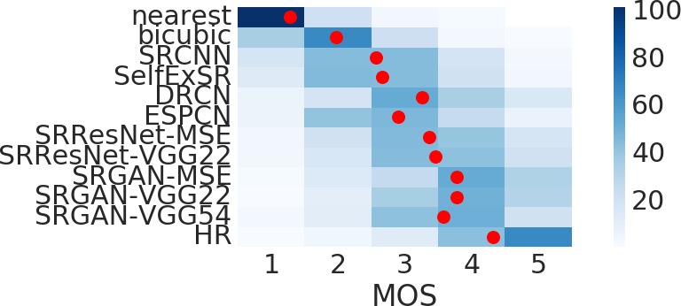
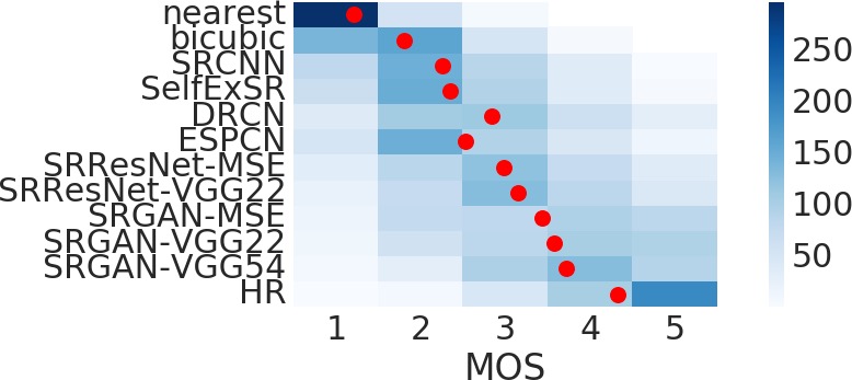
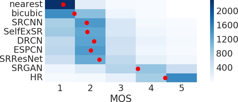
We have performed a MOS test to quantify the ability of different approaches to reconstruct perceptually convincing images. Specifically, we asked 26 raters to assign an integral score from 1 (bad quality) to 5 (excellent quality) to the super-resolved images. The raters rated 12 versions of each image on Set5, Set14 and BSD100: nearest neighbor (NN), bicubic, SRCNN [9], SelfExSR [31], DRCN [34], ESPCN [48], SRResNet-MSE, SRResNet-VGG22∗ (∗not rated on BSD100), SRGAN-MSE∗, SRGAN-VGG22∗, SRGAN-VGG54 and the original HR image. Each rater thus rated 1128 instances (12 versions of 19 images plus 9 versions of 100 images) that were presented in a randomized fashion. The raters were calibrated on the NN (score 1) and HR (5) versions of 20 images from the BSD300 training set. In a pilot study we assessed the calibration procedure and the test-retest reliability of 26 raters on a subset of 10 images from BSD100 by adding a method’s images twice to a larger test set. We found good reliability and no significant differences between the ratings of the identical images. Raters very consistently rated NN interpolated test images as 1 and the original HR images as 5 (c.f. Figure 5).
The experimental results of the conducted MOS tests are summarized in Table 1, Table 2 and Figure 5.
SRResNet- SRGAN- Set5 MSE VGG22 MSE VGG22 VGG54 PSNR 32.05 30.51 30.64 29.84 29.40 SSIM 0.9019 0.8803 0.8701 0.8468 0.8472 MOS 3.37 3.46 3.77 3.78 3.58 Set14 PSNR 28.49 27.19 26.92 26.44 26.02 SSIM 0.8184 0.7807 0.7611 0.7518 0.7397 MOS 2.98 3.15∗ 3.43 3.57 3.72∗
3.4 Investigation of content loss
We investigated the effect of different content loss choices in the perceptual loss for the GAN-based networks. Specifically we investigate for the following content losses :
-
•
SRGAN-MSE: , to investigate the adversarial network with the standard MSE as content loss.
-
•
SRGAN-VGG22: with , a loss defined on feature maps representing lower-level features [68].
- •
We also evaluate the performance of the generator network without adversarial component for the two losses (SRResNet-MSE) and (SRResNet-VGG22). We refer to SRResNet-MSE as SRResNet. Note, when training SRResNet-VGG22 we added an additional total variation loss with weight to [2, 33]. Quantitative results are summarized in Table 1 and visual examples provided in Figure 6. Even combined with the adversarial loss, MSE provides solutions with the highest PSNR values that are, however, perceptually rather smooth and less convincing than results achieved with a loss component more sensitive to visual perception. This is caused by competition between the MSE-based content loss and the adversarial loss. We further attribute minor reconstruction artifacts, which we observed in a minority of SRGAN-MSE-based reconstructions, to those competing objectives. We could not determine a significantly best loss function for SRResNet or SRGAN with respect to MOS score on Set5. However, SRGAN-VGG54 significantly outperformed other SRGAN and SRResNet variants on Set14 in terms of MOS. We observed a trend that using the higher level VGG feature maps yields better texture detail when compared to (c.f. Figure 6). Further examples of perceptual improvements through SRGAN over SRResNet are provided in the supplementary material.

| SRResNet | SRGAN-MSE | SRGAN-VGG22 | SRGAN-VGG54 | original HR image |
Set5 nearest bicubic SRCNN SelfExSR DRCN ESPCN SRResNet SRGAN HR PSNR 26.26 28.43 30.07 30.33 31.52 30.76 32.05 29.40 SSIM 0.7552 0.8211 0.8627 0.872 0.8938 0.8784 0.9019 0.8472 1 MOS 1.28 1.97 2.57 2.65 3.26 2.89 3.37 3.58 4.32 Set14 PSNR 24.64 25.99 27.18 27.45 28.02 27.66 28.49 26.02 SSIM 0.7100 0.7486 0.7861 0.7972 0.8074 0.8004 0.8184 0.7397 1 MOS 1.20 1.80 2.26 2.34 2.84 2.52 2.98 3.72 4.32 BSD100 PSNR 25.02 25.94 26.68 26.83 27.21 27.02 27.58 25.16 SSIM 0.6606 0.6935 0.7291 0.7387 0.7493 0.7442 0.7620 0.6688 1 MOS 1.11 1.47 1.87 1.89 2.12 2.01 2.29 3.56 4.46
3.5 Performance of the final networks
We compare the performance of SRResNet and SRGAN to NN, bicubic interpolation, and four state-of-the-art methods. Quantitative results are summarized in Table 2 and confirm that SRResNet (in terms of PSNR/SSIM) sets a new state of the art on three benchmark datasets. Please note that we used a publicly available framework for evaluation (c.f. Section 3.1), reported values might thus slightly deviate from those reported in the original papers.
We further obtained MOS ratings for SRGAN and all reference methods on BSD100. Examples of images super-resolved with SRResNet and SRGAN are depicted in the supplementary material. The results shown in Table 2 confirm that SRGAN outperforms all reference methods by a large margin and sets a new state of the art for photo-realistic image SR. All differences in MOS (c.f. Table 2) are highly significant on BSD100, except SRCNN vs. SelfExSR. The distribution of all collected MOS ratings is summarized in Figure 5.
4 Discussion and future work
We confirmed the superior perceptual performance of SRGAN using MOS testing. We have further shown that standard quantitative measures such as PSNR and SSIM fail to capture and accurately assess image quality with respect to the human visual system [56]. The focus of this work was the perceptual quality of super-resolved images rather than computational efficiency. The presented model is, in contrast to Shi et al. [48], not optimized for video SR in real-time. However, preliminary experiments on the network architecture suggest that shallower networks have the potential to provide very efficient alternatives at a small reduction of qualitative performance. In contrast to Dong et al. [10], we found deeper network architectures to be beneficial. We speculate that the ResNet design has a substantial impact on the performance of deeper networks. We found that even deeper networks () can further increase the performance of SRResNet, however, come at the cost of longer training and testing times (c.f. supplementary material). We further found SRGAN variants of deeper networks are increasingly difficult to train due to the appearance of high-frequency artifacts.
Of particular importance when aiming for photo-realistic solutions to the SR problem is the choice of the content loss as illustrated in Figure 6. In this work, we found to yield the perceptually most convincing results, which we attribute to the potential of deeper network layers to represent features of higher abstraction [68, 65, 40] away from pixel space. We speculate that feature maps of these deeper layers focus purely on the content while leaving the adversarial loss focusing on texture details which are the main difference between the super-resolved images without the adversarial loss and photo-realistic images. We also note that the ideal loss function depends on the application. For example, approaches that hallucinate finer detail might be less suited for medical applications or surveillance. The perceptually convincing reconstruction of text or structured scenes [31] is challenging and part of future work. The development of content loss functions that describe image spatial content, but more invariant to changes in pixel space will further improve photo-realistic image SR results.
5 Conclusion
We have described a deep residual network SRResNet that sets a new state of the art on public benchmark datasets when evaluated with the widely used PSNR measure. We have highlighted some limitations of this PSNR-focused image super-resolution and introduced SRGAN, which augments the content loss function with an adversarial loss by training a GAN. Using extensive MOS testing, we have confirmed that SRGAN reconstructions for large upscaling factors () are, by a considerable margin, more photo-realistic than reconstructions obtained with state-of-the-art reference methods.
References
- [1] J. Allebach and P. W. Wong. Edge-directed interpolation. In Proceedings of International Conference on Image Processing, volume 3, pages 707–710, 1996.
- [2] H. A. Aly and E. Dubois. Image up-sampling using total-variation regularization with a new observation model. IEEE Transactions on Image Processing, 14(10):1647–1659, 2005.
- [3] M. Bevilacqua, A. Roumy, C. Guillemot, and M. L. Alberi-Morel. Low-complexity single-image super-resolution based on nonnegative neighbor embedding. BMVC, 2012.
- [4] S. Borman and R. L. Stevenson. Super-Resolution from Image Sequences - A Review. Midwest Symposium on Circuits and Systems, pages 374–378, 1998.
- [5] J. Bruna, P. Sprechmann, and Y. LeCun. Super-resolution with deep convolutional sufficient statistics. In International Conference on Learning Representations (ICLR), 2016.
- [6] D. Dai, R. Timofte, and L. Van Gool. Jointly optimized regressors for image super-resolution. In Computer Graphics Forum, volume 34, pages 95–104, 2015.
- [7] E. Denton, S. Chintala, A. Szlam, and R. Fergus. Deep generative image models using a laplacian pyramid of adversarial networks. In Advances in Neural Information Processing Systems (NIPS), pages 1486–1494, 2015.
- [8] S. Dieleman, J. Schlüter, C. Raffel, E. Olson, S. K. Sønderby, D. Nouri, D. Maturana, M. Thoma, E. Battenberg, J. Kelly, J. D. Fauw, M. Heilman, diogo149, B. McFee, H. Weideman, takacsg84, peterderivaz, Jon, instagibbs, D. K. Rasul, CongLiu, Britefury, and J. Degrave. Lasagne: First release., 2015.
- [9] C. Dong, C. C. Loy, K. He, and X. Tang. Learning a deep convolutional network for image super-resolution. In European Conference on Computer Vision (ECCV), pages 184–199. Springer, 2014.
- [10] C. Dong, C. C. Loy, K. He, and X. Tang. Image super-resolution using deep convolutional networks. IEEE Transactions on Pattern Analysis and Machine Intelligence, 38(2):295–307, 2016.
- [11] C. Dong, C. C. Loy, and X. Tang. Accelerating the super-resolution convolutional neural network. In European Conference on Computer Vision (ECCV), pages 391–407. Springer, 2016.
- [12] W. Dong, L. Zhang, G. Shi, and X. Wu. Image deblurring and super-resolution by adaptive sparse domain selection and adaptive regularization. IEEE Transactions on Image Processing, 20(7):1838–1857, 2011.
- [13] A. Dosovitskiy and T. Brox. Generating images with perceptual similarity metrics based on deep networks. In Advances in Neural Information Processing Systems (NIPS), pages 658–666, 2016.
- [14] C. E. Duchon. Lanczos Filtering in One and Two Dimensions. In Journal of Applied Meteorology, volume 18, pages 1016–1022. 1979.
- [15] S. Farsiu, M. D. Robinson, M. Elad, and P. Milanfar. Fast and robust multiframe super resolution. IEEE Transactions on Image Processing, 13(10):1327–1344, 2004.
- [16] J. A. Ferwerda. Three varieties of realism in computer graphics. In Electronic Imaging, pages 290–297. International Society for Optics and Photonics, 2003.
- [17] W. T. Freeman, T. R. Jones, and E. C. Pasztor. Example-based super-resolution. IEEE Computer Graphics and Applications, 22(2):56–65, 2002.
- [18] W. T. Freeman, E. C. Pasztor, and O. T. Carmichael. Learning low-level vision. International Journal of Computer Vision, 40(1):25–47, 2000.
- [19] L. A. Gatys, A. S. Ecker, and M. Bethge. Texture synthesis using convolutional neural networks. In Advances in Neural Information Processing Systems (NIPS), pages 262–270, 2015.
- [20] L. A. Gatys, A. S. Ecker, and M. Bethge. Image Style Transfer Using Convolutional Neural Networks. In IEEE Conference on Computer Vision and Pattern Recognition (CVPR), pages 2414–2423, 2016.
- [21] D. Glasner, S. Bagon, and M. Irani. Super-resolution from a single image. In IEEE International Conference on Computer Vision (ICCV), pages 349–356, 2009.
- [22] I. Goodfellow, J. Pouget-Abadie, M. Mirza, B. Xu, D. Warde-Farley, S. Ozair, A. Courville, and Y. Bengio. Generative adversarial nets. In Advances in Neural Information Processing Systems (NIPS), pages 2672–2680, 2014.
- [23] K. Gregor and Y. LeCun. Learning fast approximations of sparse coding. In Proceedings of the 27th International Conference on Machine Learning (ICML-10), pages 399–406, 2010.
- [24] S. Gross and M. Wilber. Training and investigating residual nets, online at http://torch.ch/blog/2016/02/04/resnets.html. 2016.
- [25] S. Gu, W. Zuo, Q. Xie, D. Meng, X. Feng, and L. Zhang. Convolutional sparse coding for image super-resolution. In IEEE International Conference on Computer Vision (ICCV), pages 1823–1831. 2015.
- [26] P. Gupta, P. Srivastava, S. Bhardwaj, and V. Bhateja. A modified psnr metric based on hvs for quality assessment of color images. In IEEE International Conference on Communication and Industrial Application (ICCIA), pages 1–4, 2011.
- [27] H. He and W.-C. Siu. Single image super-resolution using gaussian process regression. In IEEE Conference on Computer Vision and Pattern Recognition (CVPR), pages 449–456, 2011.
- [28] K. He, X. Zhang, S. Ren, and J. Sun. Delving deep into rectifiers: Surpassing human-level performance on imagenet classification. In IEEE International Conference on Computer Vision (ICCV), pages 1026–1034, 2015.
- [29] K. He, X. Zhang, S. Ren, and J. Sun. Deep residual learning for image recognition. In IEEE Conference on Computer Vision and Pattern Recognition (CVPR), pages 770–778, 2016.
- [30] K. He, X. Zhang, S. Ren, and J. Sun. Identity mappings in deep residual networks. In European Conference on Computer Vision (ECCV), pages 630–645. Springer, 2016.
- [31] J. B. Huang, A. Singh, and N. Ahuja. Single image super-resolution from transformed self-exemplars. In IEEE Conference on Computer Vision and Pattern Recognition (CVPR), pages 5197–5206, 2015.
- [32] S. Ioffe and C. Szegedy. Batch normalization: Accelerating deep network training by reducing internal covariate shift. In Proceedings of The 32nd International Conference on Machine Learning (ICML), pages 448–456, 2015.
- [33] J. Johnson, A. Alahi, and F. Li. Perceptual losses for real-time style transfer and super- resolution. In European Conference on Computer Vision (ECCV), pages 694–711. Springer, 2016.
- [34] J. Kim, J. K. Lee, and K. M. Lee. Deeply-recursive convolutional network for image super-resolution. In IEEE Conference on Computer Vision and Pattern Recognition (CVPR), 2016.
- [35] K. I. Kim and Y. Kwon. Single-image super-resolution using sparse regression and natural image prior. IEEE Transactions on Pattern Analysis and Machine Intelligence, 32(6):1127–1133, 2010.
- [36] D. Kingma and J. Ba. Adam: A method for stochastic optimization. In International Conference on Learning Representations (ICLR), 2015.
- [37] A. Krizhevsky, I. Sutskever, and G. E. Hinton. Imagenet classification with deep convolutional neural networks. In Advances in Neural Information Processing Systems (NIPS), pages 1097–1105, 2012.
- [38] C. Li and M. Wand. Combining Markov Random Fields and Convolutional Neural Networks for Image Synthesis. In IEEE Conference on Computer Vision and Pattern Recognition (CVPR), pages 2479–2486, 2016.
- [39] X. Li and M. T. Orchard. New edge-directed interpolation. IEEE Transactions on Image Processing, 10(10):1521–1527, 2001.
- [40] A. Mahendran and A. Vedaldi. Visualizing deep convolutional neural networks using natural pre-images. International Journal of Computer Vision, pages 1–23, 2016.
- [41] D. Martin, C. Fowlkes, D. Tal, and J. Malik. A database of human segmented natural images and its application to evaluating segmentation algorithms and measuring ecological statistics. In IEEE International Conference on Computer Vision (ICCV), volume 2, pages 416–423, 2001.
- [42] M. Mathieu, C. Couprie, and Y. LeCun. Deep multi-scale video prediction beyond mean square error. In International Conference on Learning Representations (ICLR), 2016.
- [43] K. Nasrollahi and T. B. Moeslund. Super-resolution: A comprehensive survey. In Machine Vision and Applications, volume 25, pages 1423–1468. 2014.
- [44] A. Radford, L. Metz, and S. Chintala. Unsupervised representation learning with deep convolutional generative adversarial networks. In International Conference on Learning Representations (ICLR), 2016.
- [45] O. Russakovsky, J. Deng, H. Su, J. Krause, S. Satheesh, S. Ma, Z. Huang, A. Karpathy, A. Khosla, M. Bernstein, et al. Imagenet large scale visual recognition challenge. International Journal of Computer Vision, pages 1–42, 2014.
- [46] J. Salvador and E. Pérez-Pellitero. Naive bayes super-resolution forest. In IEEE International Conference on Computer Vision (ICCV), pages 325–333. 2015.
- [47] S. Schulter, C. Leistner, and H. Bischof. Fast and accurate image upscaling with super-resolution forests. In IEEE Conference on Computer Vision and Pattern Recognition (CVPR), pages 3791–3799, 2015.
- [48] W. Shi, J. Caballero, F. Huszar, J. Totz, A. P. Aitken, R. Bishop, D. Rueckert, and Z. Wang. Real-Time Single Image and Video Super-Resolution Using an Efficient Sub-Pixel Convolutional Neural Network. In IEEE Conference on Computer Vision and Pattern Recognition (CVPR), pages 1874–1883, 2016.
- [49] K. Simonyan and A. Zisserman. Very deep convolutional networks for large-scale image recognition. In International Conference on Learning Representations (ICLR), 2015.
- [50] J. Sun, J. Sun, Z. Xu, and H.-Y. Shum. Image super-resolution using gradient profile prior. In IEEE Conference on Computer Vision and Pattern Recognition (CVPR), pages 1–8, 2008.
- [51] C. Szegedy, W. Liu, Y. Jia, P. Sermanet, S. Reed, D. Anguelov, D. Erhan, V. Vanhoucke, and A. Rabinovich. Going deeper with convolutions. In IEEE Conference on Computer Vision and Pattern Recognition (CVPR), pages 1–9, 2015.
- [52] Y.-W. Tai, S. Liu, M. S. Brown, and S. Lin. Super Resolution using Edge Prior and Single Image Detail Synthesis. In IEEE Conference on Computer Vision and Pattern Recognition (CVPR), pages 2400–2407, 2010.
- [53] Theano Development Team. Theano: A Python framework for fast computation of mathematical expressions. arXiv preprint arXiv:1605.02688, 2016.
- [54] R. Timofte, V. De, and L. Van Gool. Anchored neighborhood regression for fast example-based super-resolution. In IEEE International Conference on Computer Vision (ICCV), pages 1920–1927, 2013.
- [55] R. Timofte, V. De Smet, and L. Van Gool. A+: Adjusted anchored neighborhood regression for fast super-resolution. In Asian Conference on Computer Vision (ACCV), pages 111–126. Springer, 2014.
- [56] G. Toderici, D. Vincent, N. Johnston, S. J. Hwang, D. Minnen, J. Shor, and M. Covell. Full Resolution Image Compression with Recurrent Neural Networks. arXiv preprint arXiv:1608.05148, 2016.
- [57] Y. Wang, L. Wang, H. Wang, and P. Li. End-to-End Image Super-Resolution via Deep and Shallow Convolutional Networks. arXiv preprint arXiv:1607.07680, 2016.
- [58] Z. Wang, A. C. Bovik, H. R. Sheikh, and E. P. Simoncelli. Image quality assessment: From error visibility to structural similarity. IEEE Transactions on Image Processing, 13(4):600–612, 2004.
- [59] Z. Wang, D. Liu, J. Yang, W. Han, and T. Huang. Deep networks for image super-resolution with sparse prior. In IEEE International Conference on Computer Vision (ICCV), pages 370–378, 2015.
- [60] Z. Wang, E. P. Simoncelli, and A. C. Bovik. Multi-scale structural similarity for image quality assessment. In IEEE Asilomar Conference on Signals, Systems and Computers, volume 2, pages 9–13, 2003.
- [61] C.-Y. Yang, C. Ma, and M.-H. Yang. Single-image super-resolution: A benchmark. In European Conference on Computer Vision (ECCV), pages 372–386. Springer, 2014.
- [62] J. Yang, J. Wright, T. Huang, and Y. Ma. Image super-resolution as sparse representation of raw image patches. In IEEE Conference on Computer Vision and Pattern Recognition (CVPR), pages 1–8, 2008.
- [63] Q. Yang, R. Yang, J. Davis, and D. Nistér. Spatial-depth super resolution for range images. In IEEE Conference on Computer Vision and Pattern Recognition (CVPR), pages 1–8, 2007.
- [64] R. Yeh, C. Chen, T. Y. Lim, M. Hasegawa-Johnson, and M. N. Do. Semantic Image Inpainting with Perceptual and Contextual Losses. arXiv preprint arXiv:1607.07539, 2016.
- [65] J. Yosinski, J. Clune, A. Nguyen, T. Fuchs, and H. Lipson. Understanding Neural Networks Through Deep Visualization. In International Conference on Machine Learning - Deep Learning Workshop 2015, page 12, 2015.
- [66] X. Yu and F. Porikli. Ultra-resolving face images by discriminative generative networks. In European Conference on Computer Vision (ECCV), pages 318–333. 2016.
- [67] H. Yue, X. Sun, J. Yang, and F. Wu. Landmark image super-resolution by retrieving web images. IEEE Transactions on Image Processing, 22(12):4865–4878, 2013.
- [68] M. D. Zeiler and R. Fergus. Visualizing and understanding convolutional networks. In European Conference on Computer Vision (ECCV), pages 818–833. Springer, 2014.
- [69] R. Zeyde, M. Elad, and M. Protter. On single image scale-up using sparse-representations. In Curves and Surfaces, pages 711–730. Springer, 2012.
- [70] K. Zhang, X. Gao, D. Tao, and X. Li. Multi-scale dictionary for single image super-resolution. In IEEE Conference on Computer Vision and Pattern Recognition (CVPR), pages 1114–1121, 2012.
- [71] W. Zou and P. C. Yuen. Very Low Resolution Face Recognition in Parallel Environment . IEEE Transactions on Image Processing, 21:327–340, 2012.
A Supplementary Material
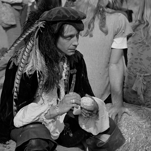
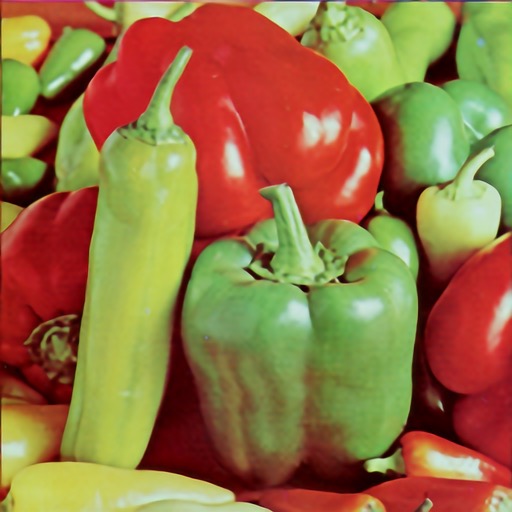
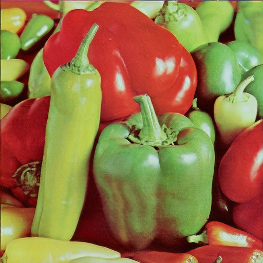
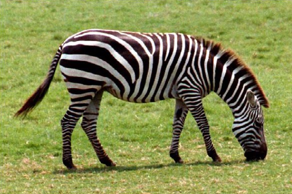
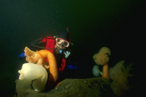
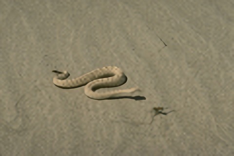
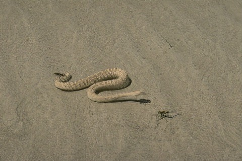
In this supplementary material we first briefly investigate the influence of network depth (number of residual blocks) on the performance (PSNR, time) of SRResNet in Section A.1. We then visualize on an example image how the SRGAN network performance evolves with increasing number of training iterations in Section A.2. Results of the MOS tests conducted on Set5, Set14, BSD100 are summarized in Section A.3. Finally we provide a visualization of all image reconstruction obtained with SRResNet and SRGAN with a upscaling factor for Set5 (Section A.4), Set14 (Section A.5) and five randomly selected images from BSD100 (Section A.6).
Images are best viewed and compared zoomed in. All original low-/high-resolution images and reconstructions ( upscaling) obtained with different methods (bicubic, SRResNet-MSE, SRResNet-VGG22, SRGAN-MSE, SRGAN-VGG22, SRGAN-VGG54) described in the paper are available for download at https://twitter.box.com/s/lcue6vlrd01ljkdtdkhmfvk7vtjhetog.
A.1 Performance (PSNR/time) vs. network depth
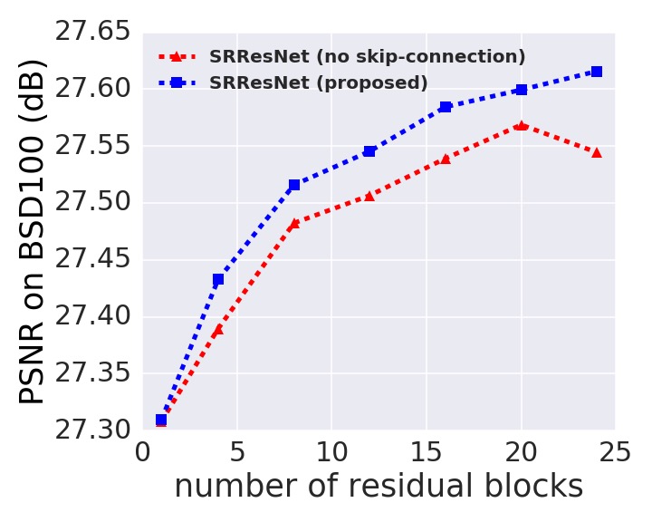
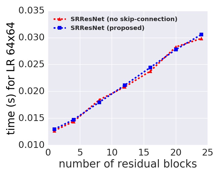
We investigated the influence of network depth, specifically the number of residual blocks, on performance (PSNR [dB] on BSD100 for SR) and inference time [s] of the network architecture described in Figure 4 of the main paper. Time was assessed on a NVIDIA M40 GPU and averaged over 100 reconstructions of a random low-resolution image with resolution 6464 with upscaling factor . The measurements are plotted in Figure 7 for a network with (blue) and without (red) skip-connection. As expected the time of a single forward pass through the network depends approximately linearly on the number of residual blocks. Whether a skip-connection is used or not has no substantial impact on inference time. However, we observed substantial gains in performance with the additional skip-connection. We chose a network architecture of 16 residual blocks with skip-connection for the evaluation presented in the main paper as we consider this as good trade-off between accuracy and speed including training time. While accuracy gains slowly saturate beyond 16 blocks there is, nevertheless, a clear benefit of using even deeper networks.
 |
 |
A.2 Evolution of Generator during SRGAN training
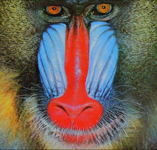
We further investigated how reconstructions of the SRGAN generator network evolve (visually) with increasing number of training iterations. Visual results obtained after different number of training iterations are illustrated in Figure 8. It is interesting that after only 20 thousand training iterations the generator substantially diverged from the SRResNet initialization and produces reconstruction with a lot of high frequency content, including noise. With increasing number of training iterations reconstructions of the baboon from Set14 appear closer to the reference image. However, there is visually little change during the last 50-100 thousand update iterations.
| SRResNet | 20k | 40k | 60k | 80k |
| 100k | 140k | 180k | SRGAN | original HR image |
A.3 Mean opinion score (MOS) testing
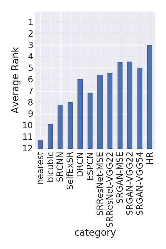
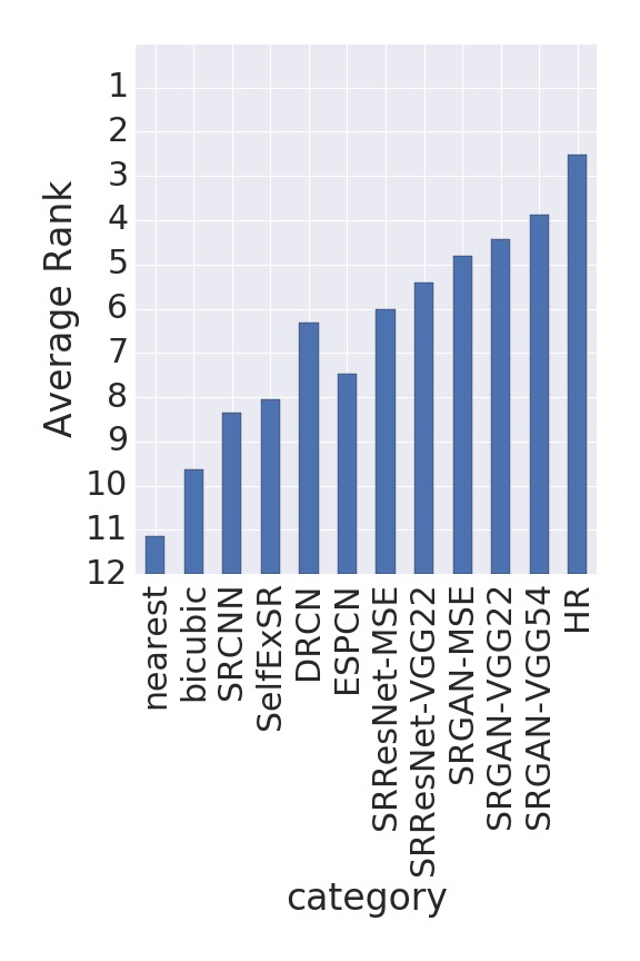
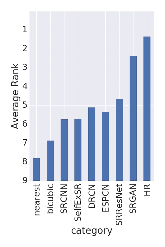
In all conducted MOS tests we have asked 26 human raters to assign a score from 1 (Bad) to 5 (Excellent) to reconstructions of the downsampled versions of images from Set5, Set14 and BSD100. On BSD100 nine versions of each image were rated by each rater. On Set5 and Set14 the raters also rated three additional versions of the proposed methods to investigate different content losses. In total 26*100*9 + 26*14*12 + 26*5*12 = 29328 ratings were obtained, where each rater rated 1128 images. Images were presented in a completely randomized fashion without any indication of the employed super-resolution approach. The raters were calibrated on images not included in the testing set such that the nearest neighbor interpolated reconstruction should receive score 1 (Bad) and the original high-resolution image score 5 (Excellent). The distribution of MOS ratings on each individual data set is summarized in Figure 9. The average ordinal rank over all corresponding ratings of an image and rater are shown in Figure 10. Note that a score of 1 corresponds to the best rank and ranks are averaged for samples that would have the same ordinal ranking. While results on Set5 are somewhat inconclusive due to very small sample size and images with comparably little detail, ratings on Set14 and especially on the large BSD100 data set confirm that SRGAN is significantly better than any compared state-of-the-art method. In fact, MOS ratings obtained with SRGAN are closer to those of the original high-resolution images than to those obtained with any reference method.
| Set5 | Set14 | BSD100 |
|---|---|---|
 |
 |
 |
| Set5 | Set14 | BSD100 |
|---|---|---|
 |
 |
 |
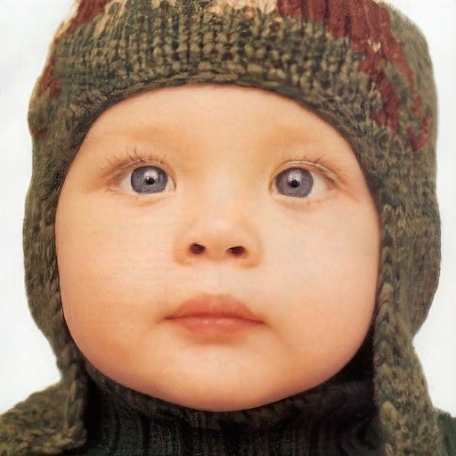
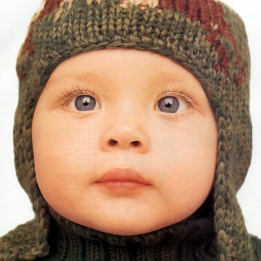
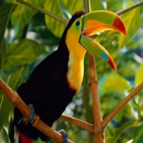
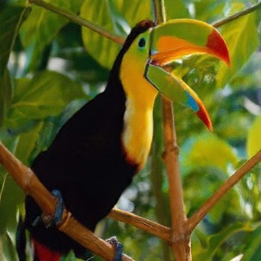
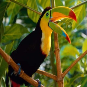
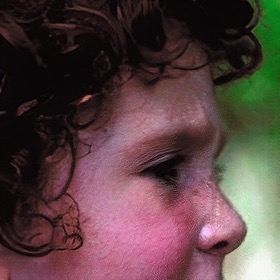
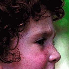
A.4 Set5 - Visual Results
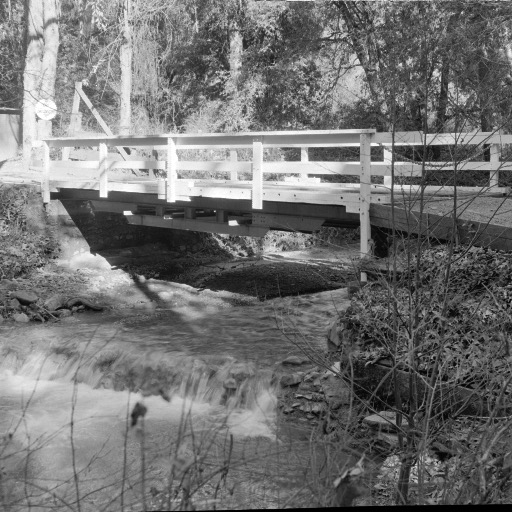
| bicubic | SRResNet | SRGAN | original |
|---|---|---|---|
 |
 |
 |
 |
 |
 |
 |
 |
 |
 |
 |
 |
 |
 |
 |
 |
 |
 |
 |
 |
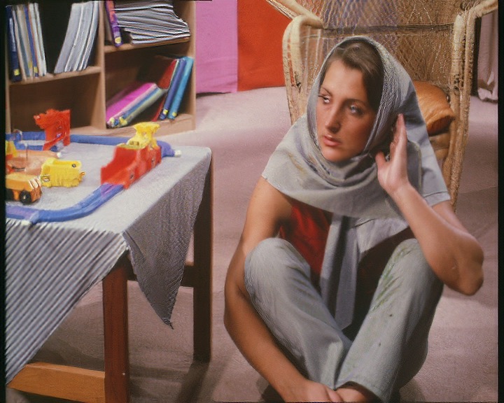
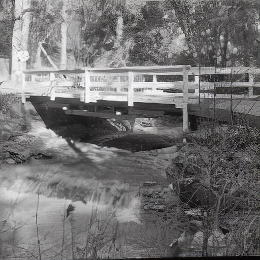
A.5 Set14 - Visual Results
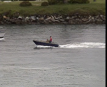
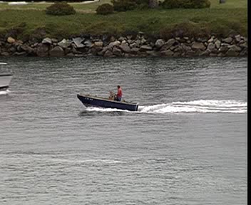
| bicubic | SRResNet | SRGAN | original |
|---|---|---|---|
 |
 |
 |
 |
 |
 |
 |
 |
 |
 |
 |
 |
 |
 |
 |
 |
 |
 |
 |
 |
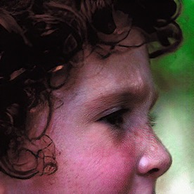
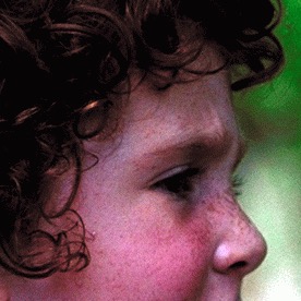
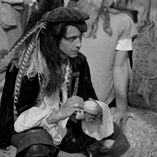
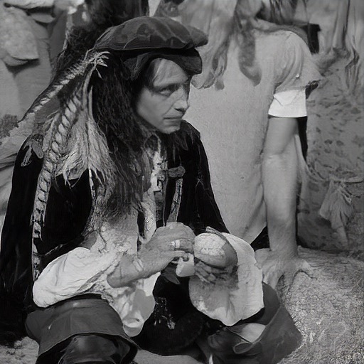
| bicubic | SRResNet | SRGAN | original |
|---|---|---|---|
 |
 |
 |
 |
 |
 |
 |
 |
 |
 |
 |
 |
 |
 |
 |
 |
 |
 |
 |
 |
| bicubic | SRResNet | SRGAN | original |
|---|---|---|---|
 |
 |
 |
 |
 |
 |
 |
 |
 |
 |
 |
 |
 |
 |
 |
 |
A.6 BSD100 (five random samples) - Visual Results
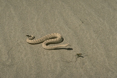
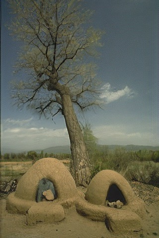
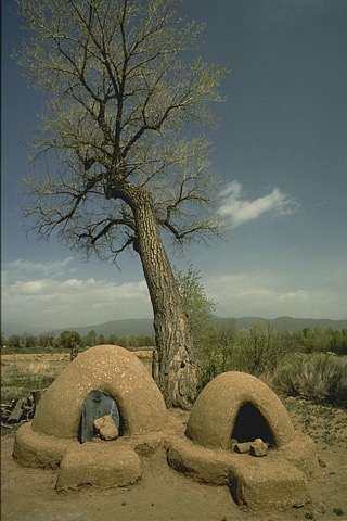
| bicubic | SRResNet | SRGAN | original |
|---|---|---|---|
 |
 |
 |
 |
 |
 |
 |
 |
 |
 |
 |
 |
 |
 |
 |
 |
 |
 |
 |
 |