GeoClaw-STRICHE: A coupled model for Sediment TRansport In Coastal Hazard Events
Abstract
STRICHE is a new model for simulating Sediment TRansport in Coastal Hazard Events, which is coupled with GeoClaw (GeoClaw-STRICHE) to provide the hydrodynamic forcing. Additionally to the standard components of sediment transport models, our models also includes sediment layers and bed avalanching to reconstruct grain-size trends as well as the generation of bed forms. Furthermore, unlike other models based on empirical equations or sediment concentration gradient, the standard Van Leer method is applied to calculate sediment flux. We tested and verified GeoClaw-STRICHE with flume experiment by Johnson et al. (2016) and data from the 2004 Indian Ocean tsunami in Kuala Meurisi as published in Apotsos et al. (2011a). The comparison with experimental and field data shows GeoClaw-STRICHE’s capability to simulate sediment thickness and grain-size distribution in experimental conditions. Model results match well with the experimental and field data, especially for sediment thickness, which builds confidence that sediment transport is correctly predicted by this model.
keywords:
Tsunami Sediment Transport , Sediment Flux , GeoClaw , Indian Ocean Tsunami1 Introduction
Recent tsunamis, such as the 2004 Indian Ocean tsunami and the 2011 Tohoku-oki tsunami, have caused approximately 420,000 deaths or missing reports and large destruction of properties in coastal communities (Apotsos et al., 2011b; Szczuciński et al., 2012). Unfortunately, tsunamis usually have long return period, which makes developing accurate tsunami hazard assessments very difficult. Therefore, to assess future events, the geologic record needs to be interrogated (Bourgeois and Minoura, 1997; Minoura et al., 2001; Jaffe and Gelfenbaum, 2002; Morton et al., 2007; Monecke et al., 2008; Szczuciński et al., 2012; Sugawara et al., 2013).
Tsunami deposits are the only recorders of past events (Huntington et al., 2007) and therefore play an important role in tsunami hazard assessments. Due to the importance of tsunami deposit, laboratory, geological and numerical modeling studies of tsunami sediment transport have been an important (Tonkin et al., 2003; Young et al., 2009, and reference therein) but often overlooked research area. Most geological methods have focused on recognizing and reconstructing the tsunami recurrence interval and characteristics of the tsunami from geological records (Jaffe and Gelfenbaum, 2002; Burroughs and Tebbens, 2005). Post-tsunami field survey can be used to interpret tsunami deposit, infer the characteristics of tsunami flow as well as verify and validate numerical models (Gelfenbaum and Jaffe, 2003; Borrero, 2005; Fritz et al., 2006; Jaffe et al., 2006; Apotsos et al., 2011b; Tappin et al., 2012; Goto et al., 2014).
As mentioned earlier,numerical modeling of tsunami sediment transport is an important research area to improve our physical understanding of tsunami hydrodynamics and sedimentology. Numerical modeling of sediment transport during tsunamis can be approached in different ways. Inversion models (e.g. Moore’s advection model, Smith’s model, Soulsby’s model, TsuSedMod, TSUFLIND, TSUFLIND-EnKF) were developed to estimate the tsunami characteristics based on tsunami deposits (Moore et al., 2007; Smith et al., 2007; Soulsby et al., 2007; Jaffe and Gelfenbuam, 2007; Tang and Weiss, 2015; Wang et al., 2015; Tang et al., 2016). On the other hand, some forward numerical models (e.g. Delft3D, Xbeach, STM, C-HYDRO3D) have been developed to study time-varying tsunami sediment transport processes (Apotsos et al., 2011a; Li et al., 2012; Ontowirjo et al., 2013; Kihara and Matsuyama, 2011; Gusman et al., 2012). Three-dimensional models with high resolution like Delft3D and C-HYDRO3D can be applied to incorporate vertical flow velocities and vertical sediment concentration profiles (Van Rijn et al., 2004; Kihara and Matsuyama, 2011). However, three-dimension models require significant computational resources when they are employed to consider geophysically meaningful domain sizes (e.g., Sugawara et al., 2014). Therefore, two-dimensional models are better suited. In most of tsunami sediment transport models (C-HYDRO3D and STM), only sediment transport with uniform particle size can be simulated (Kihara and Matsuyama, 2011; Gusman et al., 2012). In order to study sedimentary structures, mixed particle sizes and multiple sediment layers need to be incorporated into the sediment transport models.
With regard to the calculation of sediment flux, three major methods can be used: empirical formulations (STM, Gusman et al., 2012), analytical approaches based on sediment concentration gradient (Xbeach and C-HYDRO3D, Roelvink et al., 2009; Kihara and Matsuyama, 2011), and numerical models qualified unbalance between depth-averaged concentration and equilibrium concentration (Xbeach and Deft3D, Roelvink et al., 2009; Van Rijn et al., 2004). All these approaches are restricted to relatively low sediment concentration gradient and small sediment flux condition, but they are inappropriate to apply in situations at which high sediment concentration gradient and large sediment flux occur. Hence, a two-dimensional, more comprehensive and robust sediment transport model with new sediment flux calculation method is needed. In this contribution, we present such a two-dimensional fully coupled sediment transport model: GeoClaw-STRICHE.
2 Theoretical Background
Our sediment transport model, STRICHE (Sediment TRansport In Coastal Hazard Events), solves the governing advection-diffusion equation with a finite volume method, add avalanching to erosion and deposition to update the bed position. STRICHE is coupled with GeoClaw to calculate the hydrodynamics. The standard Van Leer method, which is a widely used method in computational fluid dynamics and aerospace engineering, is applied to calculate sediment flux. The bed updating and avalanching scheme from Roelvink et al. (2009) is used for updating topography during tsunami. STRICHE also includes multiple grain-size classes and sediment layers to simulate sediment structure in tsunami deposits.
2.1 Sediment Transport Model: STRICHE
2.1.1 Sediment transport condition
The critical shear velocity is employed to decide whether sediment particles in a given flow condition are entrained into the flow or not. The critical shear velocity, , is estimated with the help of an iterative procedure that discretices the Shields diagram (see Weiss, 2008). The Rouse number, , is used to determine the sediment transport condition for each grain-size class: (1) : all grains travel as bed load; (2) : parts of sediment can travel as suspended load and rest will travel as bed load (the percentages for bed and suspended load linearly depends on critical velocity); (3) : all grains travel in suspended condition. The critical velocity for bed load is given by:
| (1) |
where is the bottom roughness from MacWilliams (2004). The eddy viscosity profile from Gelfenbaum and Smith (1986) is given by:
| (2) |
in which is the elevation above bed. The critical velocity for suspended load is:
| (3) |
and
| (4) |
The combined bed and suspended load sediment concentration is updated by solving the advection-diffusion equation (Galappatti and Vreugdenhil, 1985):
| (5) |
in which is the depth-averaged sediment concentration, denotes to the sediment diffusion coefficient, refers to the adaptation time, and is the equilibrium sediment concentration.
2.1.2 Transport formulations
Two methods to calculate the equilibrium sediment concentration methods are made available in the current version of STRICHE. For both methods, the total equilibrium sediment concentration should be between maximum allowed sediment concentration, and 0. The formulae to determine the equilibrium sediment concentration are given in the following sections. It should be noted that both of these two methods are modified to distinguish between bed and suspend load. The first one is modified based on Soulsby-Van Rijn equations (Van Rijn, 1984; Soulsby, 1997). In this method, the equilibrium sediment concentration is calculated by:
| (6) |
| (7) |
The suspended load and bed load coefficient are calculated by:
| (8) |
| (9) |
where is dimensionless grain size class. The critical velocity for bed load and suspended load are calculated based on the method presented in section 2.1.1. When STRICHE deals with multiple grain-size classes, the median value of grain-size distribution, , in these equations is replaced by diameter of each grain size class. Parameter is the magnitude of the Eulerian velocity, and denotes the root-mean-squared velocity obtained from linear wave theory. For the drag coefficient is given by:
| (10) |
2.1.3 Sediment settling velocity and density effect
The calculation of the settling velocity is based on Hallermeier (1981) and Ahrens (2000). For high sediment concentration, the fall velocity is reduced:
| (15) |
in which is the total volume sediment concentration. Exponent is estimated with the help of Rowe (1987), which depends on the Reynolds particle number, :
| (16) |
| (17) |
Then bulk density of the fluid becomes a function of the water density and the sediment that is suspended in it (Warner et al., 2008):
| (18) |
In this equation, is water density, and denotes sediment concentration for grain-size class . is sediment density for grain-size class . is the total number of grain-size classes. This enables STRICHE to simulate sediment transport in high sediment concentration condition and help to extend the density stratification in the future.
2.1.4 Sediment Flux
In STRICHE, the standard Van Leer method (Van Leer, 1997) and the Monotonic Upstream-centered Scheme for Conservation Laws (MUSCL) scheme (Van Leer, 1979) are modified and applied to calculate sediment flux. The Van Leer method is a finite volume method that can provide highly accurate numerical solutions, especially for the solutions include shocks, discontinuities, or large gradient. First, the left and right states of the wave speed are determined on the cell surface in which cell surface denotes the surface between cells and by:
| (19) |
| (20) |
and refer to the left and right states of water depth on the cell surface. The right and left states of the variables are decided by the MUSCL scheme. For the first order, , . Also the left and right states of Froude number are given by:
| (21) |
| (22) |
and represent the left and right states of the depth-averaged velocity at the cell surface. After that, the positive and negative Froude numbers are given by:
| (23) |
And then parameter and are calculated:
| (24) |
| (25) |
is a function to evaluate the integer part from the variable, and is a function to return the value of the first variable with the sign of the second variable. The modified Froude number is determined:
| (26) |
Finally, the sediment flux at this cell surface is:
| (27) |
in which and are the left and right states of sediment concentration on cell surface. In order to reduce non-physical dissipation in this model, we apply sediment flux limiter in the second order simulation. Then sediment flux in y direction is calculated with the same method.
2.1.5 Sediment Flux Limiter
To reduce non-physical dissipation, limit the influence of topography change and get high order accuracy in this model, we apply sediment flux limiter and MUSCL scheme based on Van Leer (1979):
| (28) |
| (29) |
It should be noted that the sediment flux limiter limits the sediment flux by modifying the sediment concentration. Parameter is the order of accuracy. is decided by the type of scheme. The flux limiter is given by:
| (30) |
| (31) |
Where sediment concentration gradient , . The flux limiter function, , is based on Van Albada et al. (1982).
2.2 Morphology Update
During deposition or erosion, the surface elevation, , is updated by:
| (32) |
in which and are sediment flux in horizontal direction and is a morphological acceleration factor from Reniers et al. (2004). To account for the slumping of sediment during tsunami, avalanching scheme from Roelvink et al. (2009) is incorporated. When the slope between two adjacent grid cells exceeds the critical slope, sediment is exchanged between these cells to reduce the slope below the critical slope.
2.3 Sediment Setting
2.3.1 Sediment Classes
In order to be able to reproduce vertical grain-size trends, different grain-size classes need to be implemented as well as different layers of erodible bed sediments. The grain-size distributions are represented by discrete grain-size classes. It should be noted that natural sediment are most likely mixtures of cohesive and non-cohesive sediments. While sediment entrainment is affected by cohesive sediments, the influence of cohesive material on non-cohesive sediments is not trivial. A dynamical model to take cohesive sediments into account is still under development and will be included in future versions of STRICHE.
2.3.2 Sediment Layers
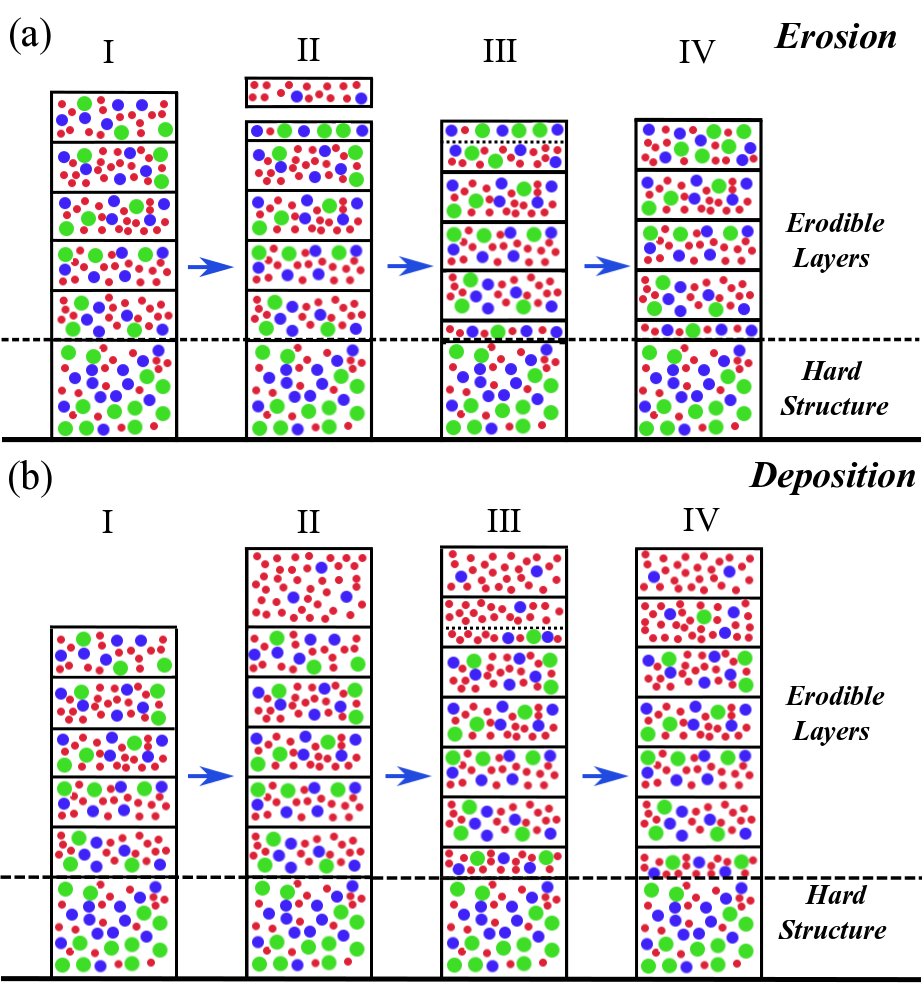
The thickness of each layer of the erodible bed is user-defined, and the top one is considered the active layer. Sediment in erodible sediment layers can be transported by suspended load and/or bed load throughout the entire simulation. However, only the sediment in the active layer is available for transport at any given time step. It is assumed that in one time step not more than the thickness of the active layer can be eroded (see Fig.1a-I & II.) After the current time step, the layers are remapped starting with the erodible bed from the top to assure that the top layer has full thickness available for erosion (see Figs.1a-II & III). A similar process is implemented for deposition as depicted in Figs.1b-I & IV. After this remapping procedure and after possible bed avalanching, the grain-size distribution in each layer are recalculated.
2.4 Hydrodynamic Model: GeoClaw
For simulating hydrodynamics of tsunami waves, GeoClaw is employed. GeoClaw is based on the Clawpack software. GeoClaw solves the nonlinear shallow water equations with high-resolution shock capturing finite volume method (Godunov-type method) on logically rectangular grids (LeVeque et al., 2011). GeoClaw also features adaptive mesh refinement (AMR) to achieve the efficient computations of large-scale geophysical problems such as tsunamis and storms. The algorithms and theories applied in GeoClaw are discussed with more details in LeVeque et al. (2011). GeoClaw is verified and validated against analytical solutions and real cases presented in González et al. (2011) and Arcos and LeVeque (2015). Furthermore, GeoClaw has been used in a number of tsunami studies and other applications (Hayes and Furlong, 2010; George, 2011; Mandli and Dawson, 2014; Adams et al., 2015).
2.5 Model algorithm
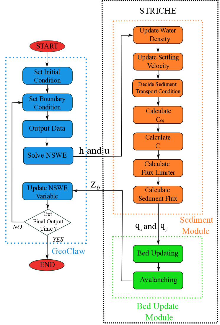
For the coupling between GeoClaw and STRICHE, a two-way coupling but separately solving system is utilized. The hydrodynamic model, sediment transport model, and morphodynamic model are constructed as three separate modules in GeoClaw-STRICHE. STRICHE includes the sediment transport model and morphodynamic model (Fig. 2). In each time step, the hydrodynamic model (GeoClaw) outputs hydrodynamic condition to the sediment transport model. The sediment transport model passes sediment fluxes to the morphodynamic model. In turn, STRICHE returns topography information to GeoClaw and change the source term of shallow water equations (Fig. 2).
3 Model Validation
In this section, we provide two validation cases that highlight the capabilities of coupled model GeoClaw-STRICHE. The first case is a flume experiment of tsunami sediment transport processes in an open channel. This case demonstrates the ability of GeoClaw-STRICHE to reproduce sediment thickness and grain-size distribution in experimental conditions. The second case is a real application with complex topography from the 2004 Indian Ocean tsunami. This case demonstrates the capability of GeoClaw-STRICHE to simulate sediment thickness in a realistic application with complex bathymetry.
3.1 Flume Experiment Case
GeoClaw-STRICHE is tested by simulating several open channel cases from Johnson et al. (2016). These laboratory experiments originally were conducted to evaluate the tsunami inversion model assumptions and qualify uncertainties. These experiment cases were set in a 32 m long, 0.5 m wide and 0.8 m high water tank at the University of Texas at Austin (Fig. 3). There was a smooth bed without slope and a lift gate to control input flow. The first three cases ran with the same grain-size distribution of the sediments (Fig. 4a, source 1) and three different initial water depths in the water tank (0, 10 and 19 cm). Case IV, V and VI set with the same initial water depth (8 cm) and three different grain-size distributions in sediment (Fig. 4a). The sediment was located between and from the lift gate, and had a trapezoidal cross section that was long and high (Fig. 3). When the gate was lifted, the flow eroded the sand dune like a tsunami would erode a coastal dune during propagation.
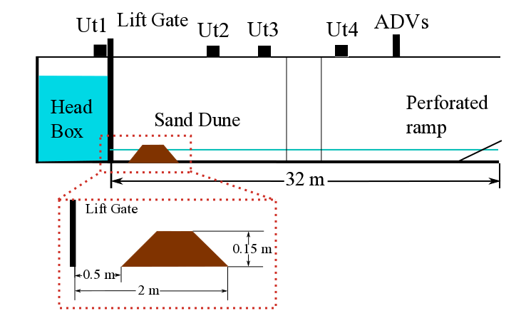
Water depth was measured at three locations (Ut2: 7.25 m, Ut3: 17.7 m and Ut4: 19.1 m from the lift gate in Fig. 3) by using ultrasonic transducers. Flow velocity was measured by two side-looking Notrek Vectrino ADVs located 19.3 m from the lift gate (Fig. 3). We calculated mean value and smoothed the original data including water depth and velocity to make them easy to compare with simulation data. After sediment deposition and water drainage, sediment thickness was measured every 25 cm. Grain-size distribution was measured every meter at 1/8 resolution by an imaged-based Retsch Camsizer. The sediment samples used to analyze grain-size distribution included the entire thickness of deposit in the sample location.
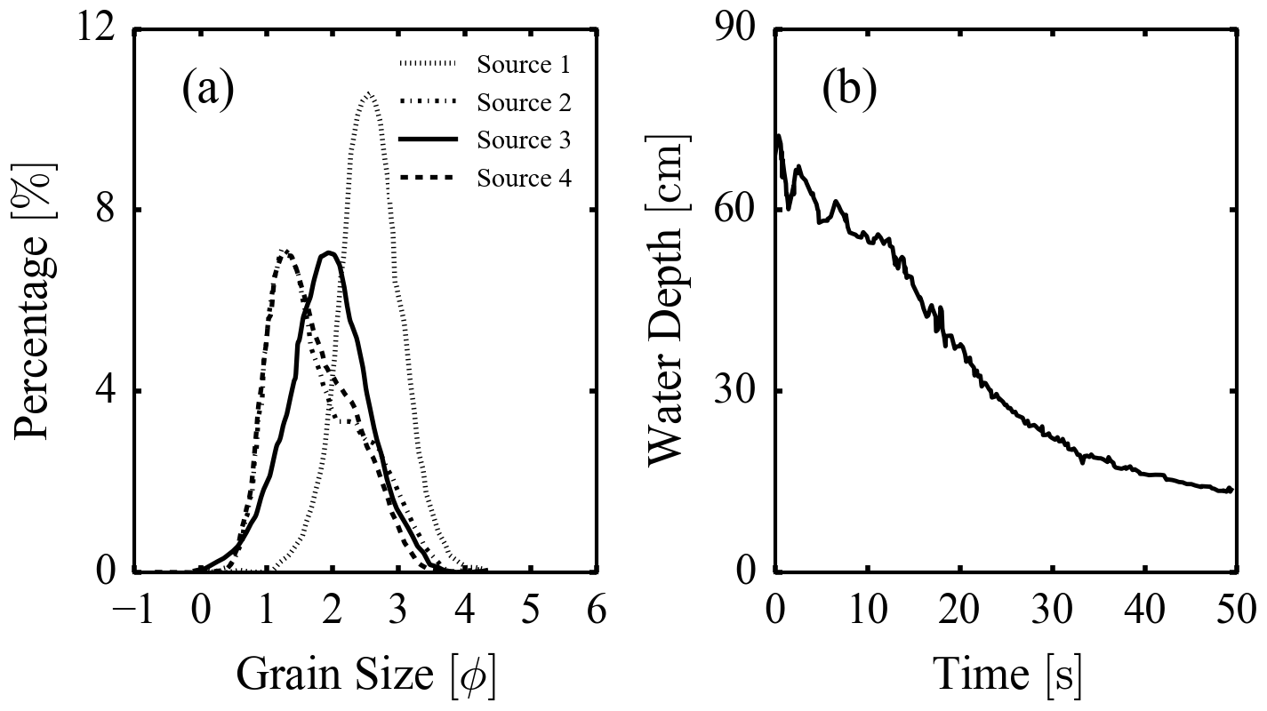
For this application, 2D depth-averaged simulations including bed load and suspended load by GeoClaw-STRICHE were carried out. The water depth at Headbox (Fig. 4b) was treated as a boundary condition in simulations. All simulations started with a sand dune located within to m from the gate (Fig. 3). Grain-size distributions of sediment were discretized with ten grain-size classes. The grain-size distributions for the experiment are depicted in Fig. 4a. The sediment layer in this case will be only separated to one erodible layer and hard structure in the model runs. The computational domain is with mesh size .
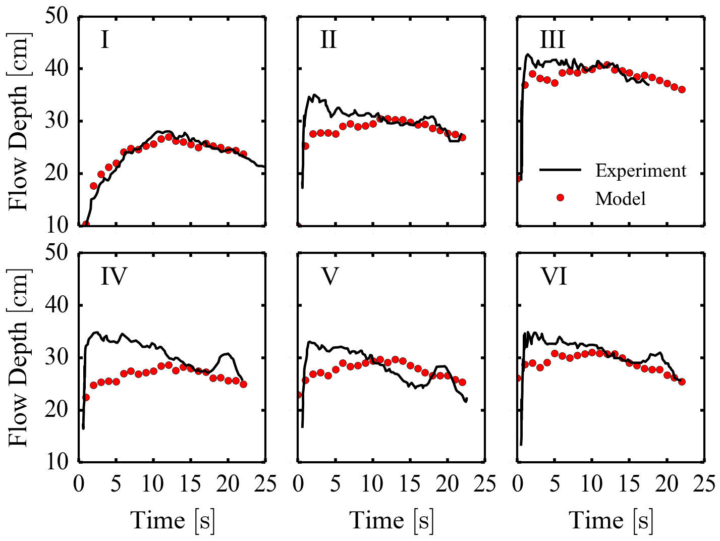
The flow depth was measured in the experiments by an ultrasonic transducer at 17.7 m downstream from the lift gate, with the exception of case III, where the flow depth was measured from sidewall with the help of video frames analysis. The experimental results from Johnson et al. (2016) show that the shallowest water depth achieved from the case I (Fig. 5-I), and deepest one achieved from case III (Fig. 5-III). The largest water depth in all cases, except case I, almost appeared immediately after bore front arrival (Figs. 5-II to 5-VI). Flow depth results from case IV to VI are very similar in the experiment as shown in Figs. 5-IV to 5-VI. For all cases, the water depth results from GeoClaw-STRICHE are in good agreements with the measurements, especially for case I. The water depth simulation results at the first ten seconds are slightly underestimated compared with experiment results for case II to VI (Figs. 5-II to 5-VI). The water depth results from 10 to 20s for case I, II, III and VI are well captured in the simulation (Figs. 5-I, II, III, VI). At the end of the simulation, calculated water depths slightly deviate from the measurement data in case IV to VI (Figs. 5-IV to VI).
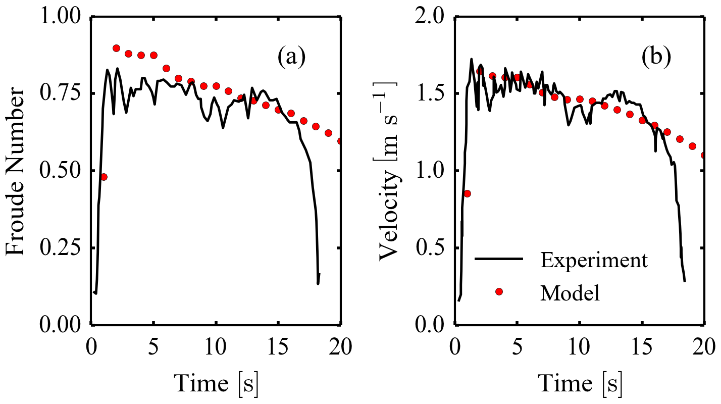
Flow velocities were measured by ADVs at from the gate. As there is little difference between velocities measured at 9 cm and 15 cm above the bed, the velocities measured in the experiment are considered as depth-averaged velocity (Johnson et al., 2016). It should be noted that the Froude number for case III is based on the flow depth at 18.7 m downstream. The flow velocity was highest right after the bore and then decreased gradually (Fig.6b). The model slightly overestimates the Froude number in the first five seconds of case III (Fig. 6a). Also the model results follow a similar pattern, but there is an obvious overprediction after 15s for both velocity and Froude number (Fig. 6).
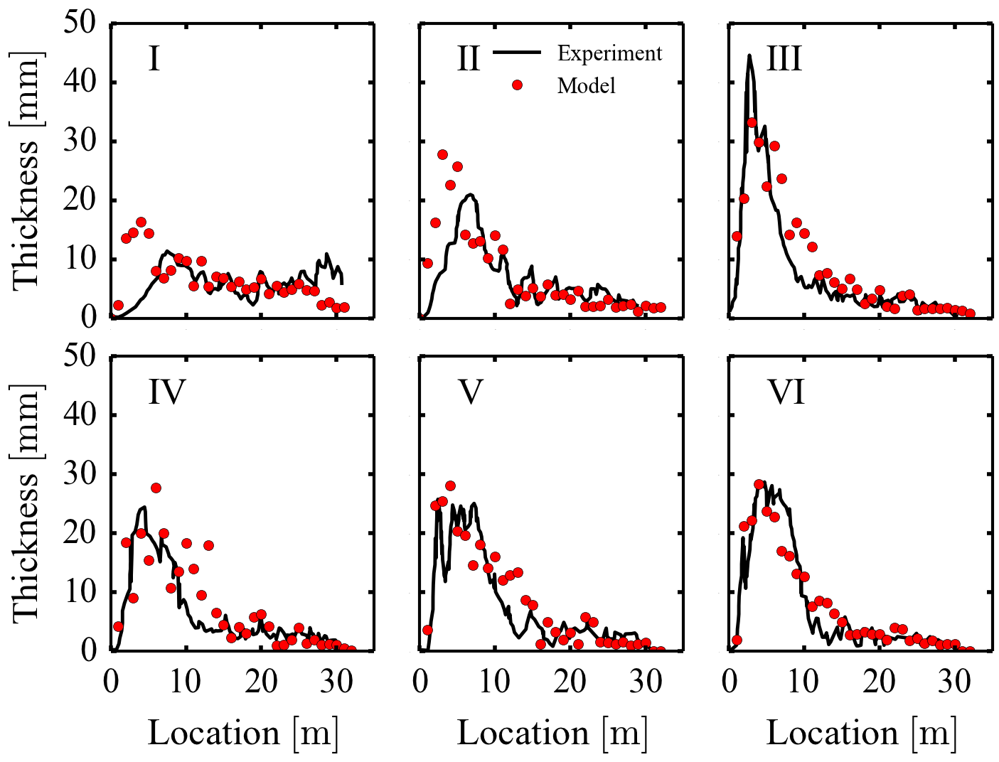
Figure 7 compares measured and calculated sediment thickness. In case I, most of the sediment dune was eroded by the flow (Fig. 7-I). For the rest of cases, the sediment thicknesses increased and then decreased. The thickness trends are not significantly different for case IV to case VI in both experimental and model results (Figs. 7-IV to VI). In most cases, the dune was significantly modified, and only a very small sediment wedge was left behind (Figs. 7-IV to VI). A significant downstream thinning of the sediment layer was observed in cases II to VI (Figs. 7-II to VI). There is again a fairly good agreement for sediment thickness between simulation and experiment in all cases (Fig. 7). The thickest sediment thickness generally occurred between and from the gate (Fig. 7).
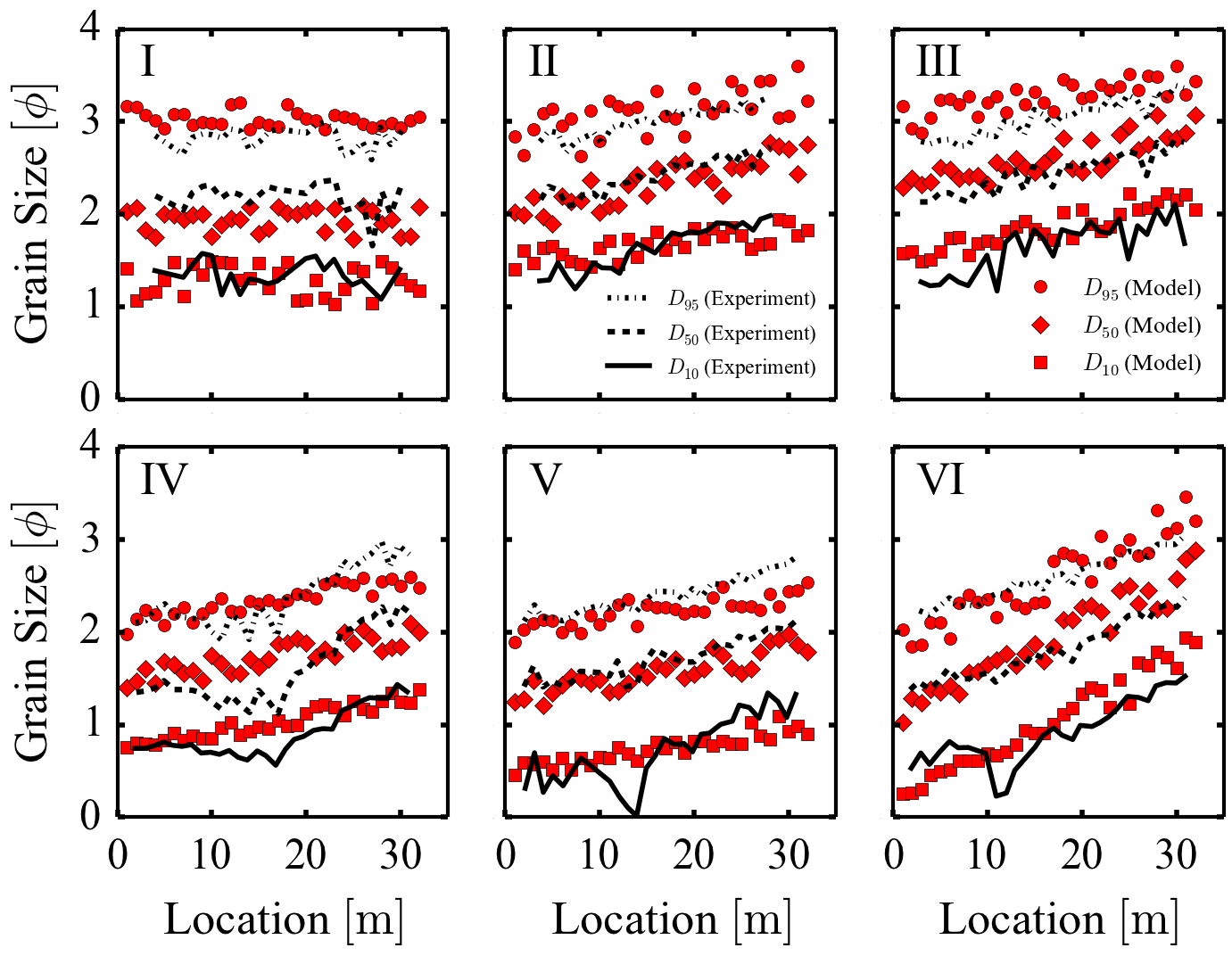
Figure 8 shows the measured and simulated , and . The trends of along the tank are very similar between experimental and simulated results for all cases. The decreases from initial dune position towards the end of tank (Fig. 8). However, the grain-size fining trend is not very obvious in case I (Fig. 8a-I). Without loss of generality, model results for fit well with experimental results. The grain-size trends are very similar for and in case II and case III (Figs. 8-II & III). The model can reproduce the and for these two cases. For cases V and VI, there is significant underprediction for and in simulations, especially for from 10 m to 20 m (Figs. 8-V & VI).
3.2 The 2004 Indian Ocean Tsunami Case
Validation data retrieved in a controlled environment does not exist for complicated topographies. Therefore, field data play a crucial role in model validation. In this section, a real case from Kuala Meurisi after the 2004 Indian Ocean tsunami is presented. Nearshore bathymetry, onshore topography and incident wave characteristics were taken from Apotsos et al. (2011a, ; red dotten line in Fig. 9a represents the pre-tsunami onland topography). A grid spacing of 10 m is used in this simulation. The erodible sediment layer is 5 m thick with five grain-size classes (-1 to 4 in scale) with equal percentages.
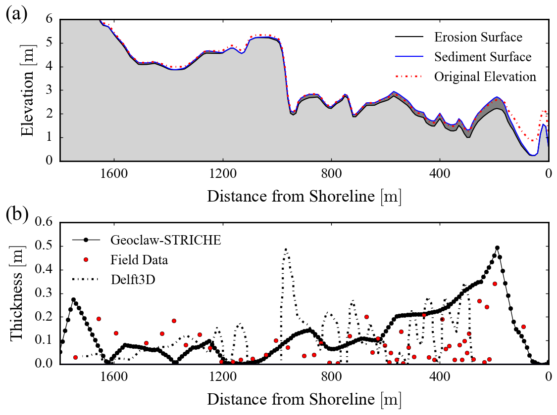
The GeoClaw-STRICHE results are compared with the field data from Kuala Meurisi and respective model results computed with Delft3D in Fig. 9. Figure 9a shows the maximum erosion surface, final sediment surface and original sediment surface. Figure 9b compares the sediment thickness along the cross section measured in the field and calculated with Delft3D (Apotsos et al., 2011a) with the results from GeoClaw-STRICHE. The results from GeoClaw-STRICHE show similar trends with the field observations. Both simulation results (GeoClaw-STRICHE and Delft3D) and field data show significant erosion in first 100 meters. In some places, such as at 150 m inland, the final sediment surface is below the original surface, but yet there is some sediment deposited, which is a model result that fits with field observation. From 200 m to 600 m inland, the model results are imperceptibly overestimated. The model results and field data fit well from 600 m to 1300 m inland. After 1300 m some underestimations appear in this area again. Compared with GeoClaw-STRICHE results, Delft3D results seem to have more fluctuations and overestimations from 200 m to 1000 m inland.
4 Discussion
4.1 Interpretation of test case results
With the help of GeoClaw-STRICHE, we can reproduce the fluid conditions as well as sediments distributions in experimental cases and real-world tsunamis. Figures 5 to 8 summarize our simulation results for the experiments. For all cases, especially for case I, model results are in very good agreement with the experiments (Figs. 5, 7, 8). The slight difference of the flow depth between model and experiment results at the first 10s for case IV to VI can be explained by the sand dune development under unsteady flow. There are obvious overpredictions after 50s for both velocity and the Froude number in Case III (Fig. 6). While this fact can arguably be ascribed to the imperfect model, we note that it is also possible that the data suffer a large uncertainty due to the fact that ADVs can return erroneous data if the flow is really shallow or a large number of air bubbles are present. Note that the Froude number in this case is calculated based on 18.7 m’s flow depth and 19.1 m’s velocity, which may also contribute to the overprediction. The thickness trends are not significantly different between case IV to VI in both experimental and model results, which indicates the grain-size distribution did not significantly control the thickness distribution for this experimental condition. However, sediment transport in the dry land condition seems to be much more difficult to simulate compared to other cases due to strong turbulence. As a result the calculated thicknesses are deviated from experiment results in Fig. 7-I. The contains apparent difference in case V and VI between observation and model results (Fig. 8). It is likely that underestimations in the fluid dynamics from model have more influence on large particles than small ones.
Figure 9 shows the model results from GeoClaw-STRICHE and Delft-3D as well as field measurement for the 2004 Indian Ocean tsunami on Kuala Meurisi. The model results show similar trends with the field measurements compared with results from Delft3D, which indicates that the strength of sediment transport is correctly predicted in GeoClaw-STRICHE for the real-world tsunami. From 200 m to 600 m inland, the model results are imperceptibly overpredicted, which may be caused by the complex topography. The fluctuations and overestimations in Delft3D’s results may due to the different way to calculate sediment thickness.
4.2 Model Limitations and Future works
The GeoClaw-STRICHE has proven its capability of simulating sediment transport by comparing experimental, field and results from Delft3D with our model. However, there are still some limitations for the present version of GeoClaw-STRICHE. A significant assumption of GeoClaw-STRICHE is that tsunami sediments are represented with several grain-size classes. As a result, the increasing number of sediment grain-size classes will significantly increase the computational load. Meanwhile, GeoClaw-STRICHE can only simulate sand sediment transport. However, tsunamis can have the power to transport almost all types of sediment from mud to boulder. Another important assumption of GeoClaw-STRICHE is that sediment will be picked up when shear velocity is larger than the critical shear velocity. In this model, we use Shield diagram to estimate the critical shear velocity for simplicity. The Shield diagram can only deal with particle size between 9 to -4 . Also the critical shear velocity from Shield diagram usually is considered as a rough estimate. At the same time, the depth-averaged velocity for sediment movement is calculated based on water depth, shear velocity and eddy viscosity profile. The choice of eddy viscosity profile will extremely influence the velocity estimation.
Future model improvement will be developed in an open source, community development approach. In order to solve computational load problems, the OpenMP and/or MPI (Message Passing Interface) should be implemented to increase calculation efficiency. Algorithms to represent cohesive sediment, gravel, and boulder sediment transport, as well as density stratification are under development. We also plan to investigate alternative approaches to calculate settling velocity, shear velocity, critical shear velocity, and sediment flux.
5 Conclusions
In this paper, we propose a tsunami sediment transport model, STRICHE. STRICHE is fully coupled with GeoClaw for computing the hydrodynamics (combined model is referred to as GeoClaw-STRICHE). STRICHE’s features include multiple sediment grain-size classes and sediment layers. The sediment concentration is computed by an advection-diffusion equation from Galappatti and Vreugdenhil (1985). The standard Van Leer method is applied for calculating sediment flux. To avoid the nonphysical model instability, a flux limiter is used. The bed-updating module controls the topography change and the mass balance between two neighbor cells. GeoClaw-STRICHE tracks sediment thickness and properties for each morphological step and updates topography information for fluid dynamic module. The quality of the matches between experimental, field and numerical results, show that STRICHE is capable of reliably simulate sediment transport during coastal hazard events, such as tsunamis. The coupling with other hydrodynamic models, for example to consider storm waves and surge, will show its capabilities for general coastal hazard flooding. Furthermore, in its current version, but especially with the planned improvement, STRICHE is and will more so be able in the future to be applied on only to modern cases, but also to coastal hazard flooding event in the past where the only physical evidence is the deposits.
Appendix A: Symbol List
| Symbol | Dimensions | Description |
| Suspended load coefficient | ||
| Bed load coefficient | ||
| Settling velocity reduction coefficient | ||
| m | Bathymetry information | |
| Depth-averaged sediment concentration | ||
| Depth-averaged sediment concentration for grain-size class m | ||
| Equilibrium depth-averaged sediment concentration | ||
| Equilibrium suspended sediment concentration | ||
| Equilibrium bed sediment concentration | ||
| Maximum allowed sediment concentration | ||
| Left or right state of depth-averaged sediment concentration | ||
| of cell surface | ||
| Depth-averaged sediment concentration for grain-size class | ||
| Depth-averaged sediment concentration at the cell (i,j) | ||
| Depth-averaged sediment concentration at the cell (i+1,j) | ||
| Drag coefficient | ||
| Left or right state of wave speed of cell surface | ||
| mm | Grain size | |
| Median Grain size | ||
| 1 | Dimensionless grain size | |
| Sediment diffusion coefficient | ||
| Left or right state of Froude number of cell surface | ||
| Plus or minus modified Froude number of cell surface | ||
| 1 | Morphological acceleration factor | |
| Gravity acceleration | ||
| m | Water depth | |
| m | Left or right state of water depth of cell surface | |
| m | Water depth at the cell (i,j) | |
| m | Water depth at the cell (i+1,j) | |
| Eddy viscosity profile | ||
| Scheme type, upwind: -1, downwind: 1 | ||
| 1 | Critical bed slope | |
| Number of grain-size classes | ||
| Rouse number | ||
| 1 | Porosity | |
| Sediment flux of cell surface | ||
| Sediment flux at x direction | ||
| Sediment flux at y direction | ||
| Reynolds particle number | ||
| Left or right state of Sediment concentration gradient of cell | ||
| surface | ||
| Adaption time | ||
| Depth-averaged velocity | ||
| Root mean square velocity | ||
| Critical velocity for bed load | ||
| Critical velocity for suspended load | ||
| Left or right state of depth-averaged velocity of cell surface | ||
| x-direction velocity | ||
| Critical shear velocity for bed load | ||
| Critical shear velocity for suspended load | ||
| y-direction velocity | ||
| Velocity magnitude | ||
| Settling velocity of the sediment grain | ||
| Reduced settling velocity of the sediment grain | ||
| m | Elevation of sediment surface | |
| Elevation from sediment bed | ||
| Bottom roughness | ||
| Settling velocity coefficient | ||
| Settling velocity coefficient | ||
| Plus or minus modified parameter of cell surface | ||
| Left or right modified parameter of cell surface | ||
| Ratio between water density and sediment density | ||
| Submerged specific gravity | ||
| Order of accuracy | ||
| Von Kaman constant | ||
| Kinematic viscosity | ||
| Sea water density | ||
| Sea water without sediment density | ||
| Sediment density for grain-size class m | ||
| Right state of flux limiter function of cell surface | ||
| Left or right state of flux limiter function of cell surface | ||
| Left state of flux limiter function of cell surface |
References
References
- Adams et al. (2015) Adams, L., LeVeque, R., and González, F. (2015). The pattern method for incorporating tidal uncertainty into probabilistic tsunami hazard assessment (PTHA). Natural Hazards, 76(1):19–39.
- Ahrens (2000) Ahrens, J. P. (2000). A fall-velocity equation. Journal of waterway, port, coastal, and ocean engineering, 126(2):99–102.
- Apotsos et al. (2011a) Apotsos, A., Gelfenbaum, G., and Jaffe, B. (2011a). Process-based modeling of tsunami inundation and sediment transport. Journal of Geophysical Research: Earth Surface, 116(F1). F01006.
- Apotsos et al. (2011b) Apotsos, A., Gelfenbaum, G., and Jaffe, B. (2011b). Process-based modeling of tsunami inundation and sediment transport. Journal of Geophysical Research: Earth Surface (2003–2012), 116(F1).
- Arcos and LeVeque (2015) Arcos, M. and LeVeque, R. J. (2015). Validating velocities in the GeoClaw tsunami model using observations near Hawaii from the 2011 Tohoku tsunami. Pure and Applied Geophysics, 172(3-4):849–867.
- Borrero (2005) Borrero, J. C. (2005). Field survey of northern Sumatra and Banda Aceh, Indonesia after the tsunami and earthquake of 26 December 2004. Seismological Research Letters, 76(3):312–320.
- Bourgeois and Minoura (1997) Bourgeois, J. and Minoura, K. (1997). Paleotsunami studies—contribution to mitigation and risk assessment. Tsunami mitigation and risk assessment, pages 1–4.
- Burroughs and Tebbens (2005) Burroughs, S. M. and Tebbens, S. F. (2005). Power-law scaling and probabilistic forecasting of tsunami runup heights. Pure and Applied Geophysics, 162(2):331–342.
- Fritz et al. (2006) Fritz, H. M., Borrero, J. C., Synolakis, C. E., and Yoo, J. (2006). 2004 Indian Ocean tsunami flow velocity measurements from survivor videos. Geophysical Research Letters, 33(24).
- Galappatti and Vreugdenhil (1985) Galappatti, G. and Vreugdenhil, C. (1985). A depth-integrated model for suspended sediment transport. Journal of Hydraulic Research, 23(4):359–377.
- Gelfenbaum and Jaffe (2003) Gelfenbaum, G. and Jaffe, B. (2003). Erosion and sedimentation from the 17 July, 1998 Papua New Guinea tsunami. In Landslide Tsunamis: Recent Findings and Research Directions, pages 1969–1999. Springer.
- Gelfenbaum and Smith (1986) Gelfenbaum, G. and Smith, J. D. (1986). Experimental evaluation of a generalized suspended-sediment transport theory. Shelf Sands and Sandstones, 1988:133–144.
- George (2011) George, D. L. (2011). Adaptive finite volume methods with well-balanced Riemann solvers for modeling floods in rugged terrain: Application to the Malpasset dam-break flood (France, 1959). International Journal for Numerical Methods in Fluids, 66(8):1000–1018.
- González et al. (2011) González, F. I., LeVeque, R. J., Chamberlain, P., Hirai, B., Varkovitzky, J., and George, D. L. (2011). Validation of the GeoClaw model. Grupo de Modelación Geoclaw Tsunami, Universidad de Washington.
- Goto et al. (2014) Goto, K., Hashimoto, K., Sugawara, D., Yanagisawa, H., and Abe, T. (2014). Spatial thickness variability of the 2011 Tohoku-oki tsunami deposits along the coastline of Sendai Bay. Marine Geology, 358:38–48.
- Gusman et al. (2012) Gusman, A. R., Tanioka, Y., and Takahashi, T. (2012). Numerical experiment and a case study of sediment transport simulation of the 2004 indian ocean tsunami in lhok nga, banda aceh, indonesia. Earth, planets and space, 64(10):817–827.
- Hallermeier (1981) Hallermeier, R. J. (1981). Terminal settling velocity of commonly occurring sand grains. Sedimentology, 28(6):859–865.
- Hayes and Furlong (2010) Hayes, G. P. and Furlong, K. P. (2010). Quantifying potential tsunami hazard in the Puysegur subduction zone, south of New Zealand. Geophysical Journal International, 183(3):1512–1524.
- Huntington et al. (2007) Huntington, K., Bourgeois, J., Gelfenbaum, G., Lynett, P., Jaffe, B., Yeh, H., and Weiss, R. (2007). Sandy signs of a tsunami’s onshore depth and speed. Eos, 88(52):577–578.
- Jaffe et al. (2006) Jaffe, B. E., Borrero, J. C., Prasetya, G. S., Peters, R., McAdoo, B., Gelfenbaum, G., Morton, R., Ruggiero, P., Higman, B., Dengler, L., et al. (2006). Northwest Sumatra and offshore islands field survey after the December 2004 Indian ocean tsunami. Earthquake Spectra, 22(S3):105–135.
- Jaffe and Gelfenbaum (2002) Jaffe, B. E. and Gelfenbaum, G. (2002). Using tsunami deposits to improve assessment of tsunami risk. Solutions to Coastal Disasters, 2:836–847.
- Jaffe and Gelfenbuam (2007) Jaffe, B. E. and Gelfenbuam, G. (2007). A simple model for calculating tsunami flow speed from tsunami deposits. Sedimentary Geology, 200(3):347–361.
- Johnson et al. (2016) Johnson, J. P., Delbecq, K., Kim, W., and Mohrig, D. (2016). Experimental tsunami deposits: Linking hydrodynamics to sediment entrainment, advection lengths and downstream fining. Geomorphology, 253:478–490.
- Kihara and Matsuyama (2011) Kihara, N. and Matsuyama, M. (2011). Numerical simulations of sediment transport induced by the 2004 indian ocean tsunami near kirinda port in sri lanka. Coastal Engineering Proceedings, 1(32):12.
- LeVeque et al. (2011) LeVeque, R. J., George, D. L., and Berger, M. J. (2011). Tsunami modelling with adaptively refined finite volume methods. Acta Numerica, 20:211–289.
- Li et al. (2012) Li, L., Huang, Z., Qiu, Q., Natawidjaja, D. H., and Sieh, K. (2012). Tsunami-induced coastal change: scenario studies for painan, west sumatra, indonesia. Earth, planets and space, 64(10):799–816.
- MacWilliams (2004) MacWilliams, M. L. (2004). Three-dimensional hydrodynamic simulation of river channels and floodplains. PhD thesis, Stanford University.
- Mandli and Dawson (2014) Mandli, K. T. and Dawson, C. N. (2014). Adaptive mesh refinement for storm surge. Ocean Modelling, 75:36 – 50.
- Minoura et al. (2001) Minoura, K., Imamura, F., Sugawara, D., Kono, Y., and Iwashita, T. (2001). The 869 Jogan tsunami deposit and recurrence interval of large-scale tsunami on the Pacific coast of northeast Japan.
- Monecke et al. (2008) Monecke, K., Finger, W., Klarer, D., Kongko, W., McAdoo, B. G., Moore, A. L., and Sudrajat, S. U. (2008). A 1,000-year sediment record of tsunami recurrence in northern Sumatra. Nature, 455(1).
- Moore et al. (2007) Moore, A. L., McAdoo, B. G., and Ruffman, A. (2007). Landward fining from multiple sources in a sand sheet deposited by the 1929 Grand Banks tsunami, Newfoundland. Sedimentary Geology, 200(3–4):336 – 346.
- Morton et al. (2007) Morton, R. A., Gelfenbaum, G., and Jaffe, B. E. (2007). Physical criteria for distinguishing sandy tsunami and storm deposits using modern examples. Sedimentary Geology, 200(3):184–207.
- Ontowirjo et al. (2013) Ontowirjo, B., Paris, R., and Mano, A. (2013). Modeling of coastal erosion and sediment deposition during the 2004 indian ocean tsunami in lhok nga, sumatra, indonesia. Natural hazards, 65(3):1967–1979.
- Reniers et al. (2004) Reniers, A. J., Roelvink, J., and Thornton, E. (2004). Morphodynamic modeling of an embayed beach under wave group forcing. Journal of Geophysical Research: Oceans, 109(C1).
- Roelvink et al. (2009) Roelvink, D., Reniers, A., Van Dongeren, A., de Vries, J. v. T., McCall, R., and Lescinski, J. (2009). Modelling storm impacts on beaches, dunes and barrier islands. Coastal engineering, 56(11):1133–1152.
- Rowe (1987) Rowe, P. (1987). A convenient empirical equation for estimation of the Richardson-Zaki exponent. Chemical Engineering Science, 42(11):2795–2796.
- Smith et al. (2007) Smith, D., Foster, I., Long, D., and Shi, S. (2007). Reconstructing the pattern and depth of flow onshore in a palaeotsunami from associated deposits. Sedimentary Geology, 200(3–4):362 – 371.
- Soulsby (1997) Soulsby, R. (1997). Dynamics of marine sands: a manual for practical applications. Thomas Telford.
- Soulsby et al. (2007) Soulsby, R., Smith, D., and Ruffman, A. (2007). Reconstructing Tsunami Run-Up from Sedimentary Characteristics: A Simple Mathematical Model, chapter 83, pages 1075–1088.
- Sugawara et al. (2014) Sugawara, D., Goto, K., and Jaffe, B. E. (2014). Numerical models of tsunami sediment transport: current understanding and future directions. Marine Geology, 352:295–320.
- Sugawara et al. (2013) Sugawara, D., Imamura, F., Goto, K., Matsumoto, H., and Minoura, K. (2013). The 2011 Tohoku-oki earthquake tsunami: similarities and differences to the 869 Jogan tsunami on the Sendai plain. Pure and Applied Geophysics, 170(5):831–843.
- Szczuciński et al. (2012) Szczuciński, W., Kokociński, M., Rzeszewski, M., Chagué-Goff, C., Cachão, M., Goto, K., and Sugawara, D. (2012). Sediment sources and sedimentation processes of 2011 Tohoku-oki tsunami deposits on the Sendai Plain, Japan—insights from diatoms, nannoliths and grain size distribution. Sedimentary Geology, 282:40–56.
- Tang et al. (2016) Tang, H., Wang, J., Weiss, R., and Xiao, H. (2016). TSUFLIND-EnKF inversion model applied to tsunami deposits for estimation of transient flow depth and speed with quantified uncertainties. arXiv preprint.
- Tang and Weiss (2015) Tang, H. and Weiss, R. (2015). A model for tsunami flow inversion from deposits (TSUFLIND). Marine Geology, 370:55–62.
- Tappin et al. (2012) Tappin, D. R., Evans, H. M., Jordan, C. J., Richmond, B., Sugawara, D., and Goto, K. (2012). Coastal changes in the sendai area from the impact of the 2011 Tōhoku-oki tsunami: Interpretations of time series satellite images, helicopter-borne video footage and field observations. Sedimentary Geology, 282:151–174.
- Tonkin et al. (2003) Tonkin, S., Yeh, H., Kato, F., and Sato, S. (2003). Tsunami scour around a cylinder. Journal of Fluid Mechanics, 496:165–192.
- Van Albada et al. (1982) Van Albada, G., Van Leer, B., and Roberts Jr, W. (1982). A comparative study of computational methods in cosmic gas dynamics. Astronomy and Astrophysics, 108:76–84.
- Van Leer (1979) Van Leer, B. (1979). Towards the ultimate conservative difference scheme. V. A second-order sequel to Godunov’s method. Journal of computational Physics, 32(1):101–136.
- Van Leer (1997) Van Leer, B. (1997). Flux-vector splitting for the euler equation. In Upwind and High-Resolution Schemes, pages 80–89. Springer.
- Van Rijn et al. (2004) Van Rijn, L., Walstra, D., and Van Ormondt, M. (2004). Description of transpor 2004 (tr2004) and implementation in delft3d online, rep. Z3748, Delft Hydraulics, Delft, The Netherlands.
- Van Rijn (1984) Van Rijn, L. C. (1984). Sediment transport, part III: bed forms and alluvial roughness. Journal of hydraulic engineering, 110(12):1733–1754.
- Van Rijn (2007) Van Rijn, L. C. (2007). Unified view of sediment transport by currents and waves. II: Suspended transport. Journal of Hydraulic Engineering.
- Van Thiel de Vries (2009) Van Thiel de Vries, J. (2009). Dune erosion during storm surges. PhD thesis, TU Delft, Delft University of Technology.
- Wang et al. (2015) Wang, J.-X., Tang, H., Xiao, H., and Weiss, R. (2015). Inversion of tsunamis characteristics from sediment deposits based on Ensemble Kalman Filtering. arXiv preprint arXiv:1511.03307.
- Warner et al. (2008) Warner, J. C., Sherwood, C. R., Signell, R. P., Harris, C. K., and Arango, H. G. (2008). Development of a three-dimensional, regional, coupled wave, current, and sediment-transport model. Computers & Geosciences, 34(10):1284–1306.
- Weiss (2008) Weiss, R. (2008). Sediment grains moved by passing tsunami waves: Tsunami deposits in deep water. Marine Geology, 250(3):251–257.
- Young et al. (2009) Young, Y. L., White, J. A., Xiao, H., and Borja, R. I. (2009). Liquefaction potential of coastal slopes induced by solitary waves. Acta Geotechnica, 4(1):17–34.