Complete reionization constraints from Planck 2015 polarization
Abstract
We conduct an analysis of the Planck 2015 data that is complete in reionization observables from the large angle polarization -mode spectrum in the redshift range . Based on 5 principal components, all of which are constrained by the data, this single analysis can be used to infer constraints on any model for reionization in the same range; we develop an effective likelihood approach for applying these constraints to models. By allowing for an arbitrary ionization history, this technique tests the robustness of inferences on the total optical depth from the usual steplike transition assumption, which is important for the interpretation of many other cosmological parameters such as the dark energy and neutrino mass. The Planck 2015 data not only allow a high redshift component to the optical depth but prefer it at the level. This preference is associated with excess power in the multipole range and may indicate high redshift ionization sources or unaccounted for systematics and foregrounds in the 2015 data.
I Introduction
The epoch of reionization of the Universe remains one of the least well-understood aspects of the standard model of cosmology (see e.g. Mesinger (2016)). Yet its impact on the interpretation of its fundamental properties is comparatively large in this era of precision cosmology. In addition to the intrinsic astrophysical interest in ionization sources, reionization uncertainties impact cosmic microwave background (CMB) inferences on the initial power spectrum and hence also cosmic acceleration through the growth of structure Hu and Jain (2004). In the future it will be one of the leading sources of error in the interpretation of neutrino mass measurements from gravitational lensing Smith et al. (2006); Allison et al. (2015), the study of large scale anomalies in the CMB Mortonson and Hu (2009); Mortonson et al. (2009), and the inflationary consistency relation Mortonson and Hu (2008a).
The standard approach to parametrizing the impact of reionization on the CMB is with the total Thomson optical depth through the reionization epoch. Although it is indeed the total optical depth that is important for the interpretation of most other aspects of cosmology, it is usually assumed that reionization occurs promptly in a steplike transition. Interestingly, the central value of the inferred optical depth from this approach has been steadily drifting downwards from its first detection in WMAP1 Kogut et al. (2003) to the current but still proprietary Planck 2016 High Frequency Instrument (HFI) results Aghanim et al. (2016); Adam et al. (2016).
Relaxing this sharp transition assumption can in principle raise the optical depth inference from the CMB as well as change its implications for sources of high redshift ionization (e.g. Ahn et al. (2012)). In particular, the angular scale of the peak and the width of the reionization bump in the -mode CMB polarization power spectrum carries coarse grained information on the redshift dependence of the ionization history.
There is an alternate, model independent approach introduced in Ref. Hu and Holder (2003) that fully addresses these concerns. The impact of any ionization history on the large angle CMB polarization spectrum can be completely characterized by a handful of reionization parameters constructed from the principal components (PCs) of the ionization history with respect to the -mode power spectrum. This approach has the advantage over redshift binning alternatives of being observationally complete without introducing numerous highly correlated parameters Lewis et al. (2006). Conversely, it does not provide an accurate, local reconstruction for visualizing the ionization history itself.
This approach was implemented and tested on WMAP3 Mortonson and Hu (2008b) and WMAP5 Mortonson and Hu (2008c) power spectra which showed that those data allowed for, but did not particularly favor, contributions to the optical depth from high redshift. It was adopted in the Planck 2013 analysis but exclusively to test the impact of marginalizing the ionization history on inflationary parameters rather than drawing inferences on reionization itself Ade et al. (2014). The impact on massive neutrinos and gravitational wave inferences was also examined in Ref. Dai et al. (2015).
In this work, we analyze the public Planck 2015 data, including the Low Frequency Instrument (LFI) large angle polarization power spectrum, using the observationally complete PC basis. In addition we further develop the technique as a method to probe reionization itself. This development is timely as the technique should come to its full fruition with the upcoming final release of Planck data which will be the definitive result on large angle polarization for years to come.
We demonstrate that the Planck 2015 data already have more information on the ionization history than just the total optical depth and provide effective likelihood tools for interpreting this information in any given model for reionization within the redshift range analyzed. Tested here, these techniques can be straightforwardly applied to the final release when it becomes available.
We begin with a review of the approach itself in Sec. II. In Sec. III, we analyze the Planck 2015 data and explore the origin of the additional information on the high redshift ionization history. We develop and test an effective likelihood approach for utilizing our analysis to constrain the parameters of any given model of reionization from in Sec. IV. We discuss these results in Sec. V.
II Complete Reionization Basis
We briefly summarize the principal component technique for the complete characterization of reionization constraints from the large angle polarization spectrum as introduced in Ref. Hu and Holder (2003) and implemented in Mortonson and Hu (2008c, b).
We parametrize the ionization fraction relative to fully ionized hydrogen into its principal components with respect to the -mode polarization of the CMB (Hu and Holder, 2003):
| (1) |
Here are the PC amplitudes and are the eigenfunctions of the Fisher information matrix for in a given range from cosmic variance limited measurements, and is the fiducial model around which the Fisher matrix is computed. In practice, we discretize the redshift space to , well beyond the resolution limit of CMB observables, and assume linear interpolation between points to form the continuous functions . The components are rank ordered by their Fisher-estimated variances and in practice the first 5 components carry all the information in to the cosmic variance limit Hu and Holder (2003). In this work, we therefore truncate the PC expansion and retain 5 parameters to describe reionization. We take to be consistent with Ly forest constraints (e.g. Becker et al. (2015)) and .
In this truncated representation, the 5 PC decomposition is not complete in the ionization history itself. Instead it is a complete representation of the observable impact on of any given through its projection onto the 5 PC basis
| (2) |
When reconstructed through Eq. (1) with 5 PCs, , even though it models the observables to high precision. The PC analysis therefore is a forward tool to infer constraints on all possible ionization histories between with a single analysis, not an inverse tool that reconstructs the ionization history.
We use a modified version of CAMB111CAMB: http://camb.info Lewis et al. (2000); Howlett et al. (2012) to compute the CMB power spectra given the ionization history. Because CAMB integrates the Boltzmann equation by parts, it requires a smooth ionization history for numerical stability, whereas the are continuous but not smooth. Consequently we smooth the ionization history in Eq. (1) with a Gaussian in of width . This does not affect our results in a statistically significant way. However for consistency, when integrating the ionization history to form the cumulative Thomson optical depth
| (3) |
we employ the smoothed which formally has support beyond the bounds. We include this small correction by integrating slightly past in practice. Here is the hydrogen number density at .
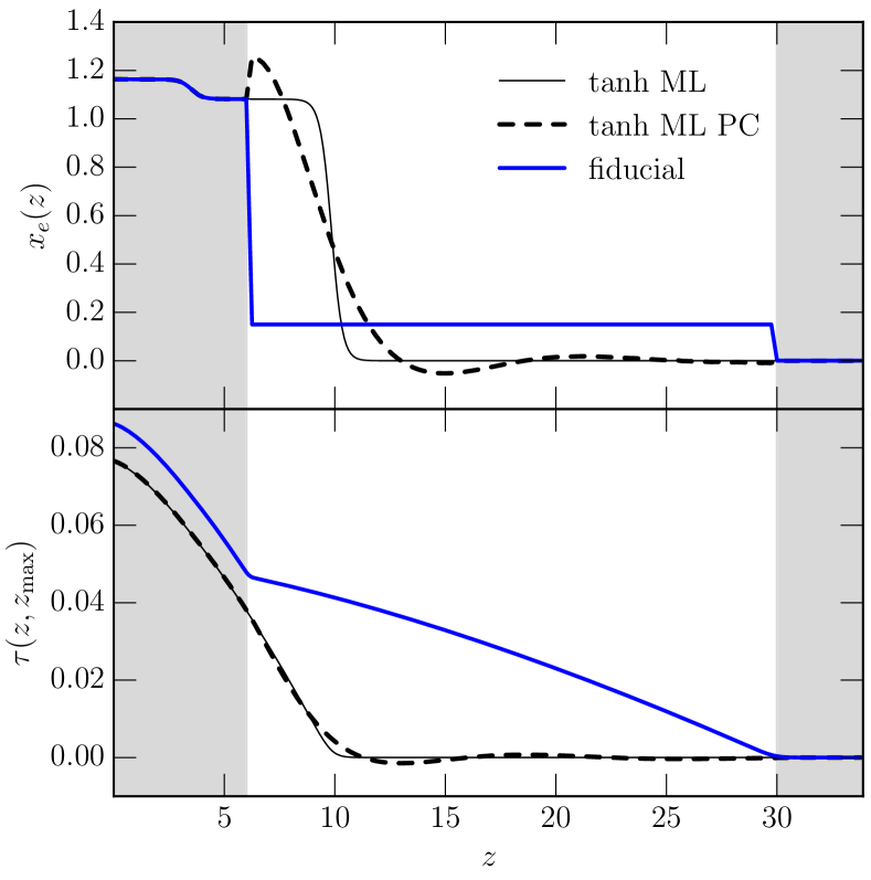
For the fiducial ionization history, we take for on the spaced discrete points in the interval with linear interpolation in between, in order to let the PC amplitudes fluctuate the ionization history both up and down without entering the unphysical region , where the number is chosen to give a reasonable . It is important to note that the PCs allow arbitrarily large deviations from the fiducial model, and so this choice does not bias results. For we assume follows the ionization history from recombination. For we assume fully ionized hydrogen and singly ionized helium
| (4) |
for and doubly ionized helium
| (5) |
for , where
| (6) |
is the ratio of the helium to hydrogen number density. We take the helium mass fraction to be consistent with big bang nucleosynthesis given the baryon density. Following CAMB, we take this helium reionization transition to be mediated by a tanh function in redshift centered at Becker et al. (2011) with width .
In Fig. 1, we show the fiducial ionization history (thick blue) and contrast it with the standard approach of CAMB (thin black) that takes hydrogen and singly ionized helium reionization to be given by the tanh form
| (7) |
with , , and . We take here , corresponding the chain maximum likelihood (ML) model () from §III, for illustrative purposes. Projected onto 5 PCs and resummed into , Eq. (1) yields a poor reconstruction of the ionization history itself. Nonetheless as we shall see in Fig. 9, the PC decomposition provides an excellent representation of the polarization power spectrum.
We also show in Fig. 1 the cumulative optical depth from to . Although the two models have comparable total optical depth the fiducial model receives much of its contribution from high redshift. Note also that although we do not allow for uncertainties in helium reionization, its entire impact is a small correction on an already small contribution to . Furthermore, although the reconstruction of using 5 PCs is still imperfect (black dashed line), it is much better than as it is more closely related to the polarization observables. The PC reconstruction smooths out sharp transitions in the cumulative optical depth but gives an accurate representation of the high and low redshift contributions of the model. In the analysis below, in order to compare exactly the same statistic between models, we always employ the PC reconstructed version.
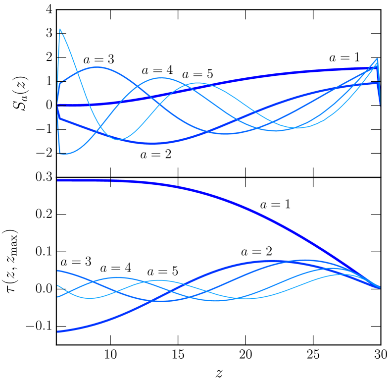
In Fig. 2 we show the 5 PC ionization functions which allow observationally complete variations around the fiducial model. We also show the cumulative optical depth for a unit amplitude in each mode. The lowest-variance eigenmode adjusts the total optical depth, mainly from the high redshift end. The mode allows a redistribution of the optical depth between high redshift and low redshift. The higher modes allow finer adjustments in the redshift distribution of the optical depth and carry very little total optical depth .
For the Planck data set, most of the information in the ionization history is carried by the first two modes and therefore relates to the amount of high vs. low redshift optical depth. We keep all 5 PCs for completeness in representing the observable impact of a given ionization history and to marginalize uncertainties that they introduce.
In fact, PCs with no prior constraints on the mode amplitudes allow deviations that are unphysical and . With a truncation at 5 PCs, physicality cannot be strictly enforced since the missing eigenmodes, while irrelevant for the observables, can restore physicality of a model. We follow Ref. Mortonson and Hu (2008c) in placing necessary but not sufficient conditions for physicality
| (8) |
where and with
| (9) |
In principle but in practice for compatibility with the ionization state at we take . Since this prior is applied very conservatively as a necessary condition, we in fact still allow ionization fractions out beyond the true maximum with this prior.
For analyzing any physical model of hydrogen reionization, , using our 5 PC decomposition from Eq. (2), the priors are noninformative as they are automatically satisfied. We apply them mainly for visualizing whether the data constrain the mode amplitudes significantly better than the physicality bounds.
III Reionization Constraints
We use the Markov Chain Monte Carlo (MCMC) technique employing a modified version of COSMOMC222COSMOMC: http://cosmologist.info/cosmomc Lewis (2013); Lewis and Bridle (2002) to sample from the posterior probability density in the reionization and cosmological parameter space. Our main analysis is on the Planck 2015 data Aghanim et al. (2015) using the public likelihoods plik_lite_TTTEEE for high-’s and lowTEB for low-’s, which includes LFI but not HFI polarization.333We have tested that our results are robust to explicitly marginalizing foreground parameters, as opposed to using the premarginalized likelihood, by separately running a PC MCMC using the lowTEB low- likelihood and the plikHM high- likelihood. For our cosmological parameters, we vary the base set of CDM parameters (baryon density , cold dark matter density , effective acoustic scale , scalar power spectrum amplitude and tilt ). We fix the neutrinos to their minimal contribution of one massive species with eV. To those parameters we add the 5 PC mode amplitudes . For comparison we also run a separate chain with the standard tanh ionization history, parametrized by the total reionization optical depth . We assume flat priors in each of the given parameters.
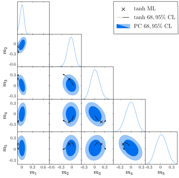
In Fig. 3, we show the 1D and 2D marginalized posteriors in the PC amplitudes and for comparison the standard tanh ionization history with 68% and 95% ranges in its parameter projected onto the PCs. Box bounds represent the physicality prior from Eq. (9). In Table 1 we give the corresponding means , errors and correlation matrix which define the covariance matrix as
| (10) |
Note that although the PCs are constructed to be uncorrelated for infinitesimal deviations from the fiducial model, they do not remain so for finite deviations (see Mortonson and Hu (2008c)).
| 0.002 | 0.053 | 1.000 | 0.450 | 0.432 | 0.273 | 0.073 | |
| 0.030 | 0.101 | 0.450 | 1.000 | 0.262 | 0.055 | 0.072 | |
| 0.019 | 0.128 | 0.432 | 0.262 | 1.000 | 0.417 | 0.155 | |
| 0.012 | 0.143 | 0.273 | 0.055 | 0.417 | 1.000 | 0.428 | |
| 0.026 | 0.143 | 0.073 | 0.072 | 0.155 | 0.428 | 1.000 |
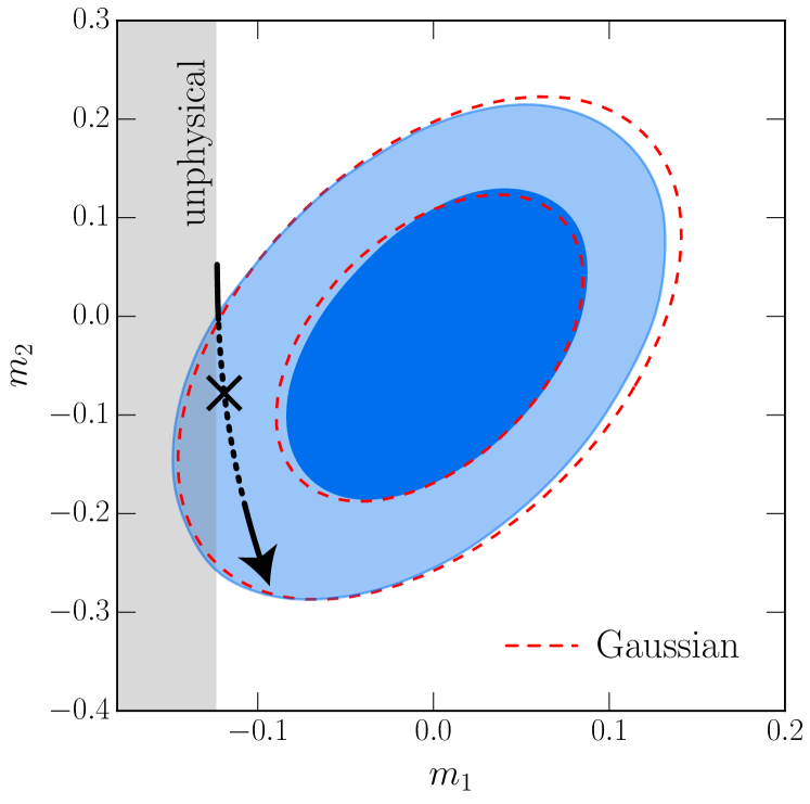
Although all 5 PCs are measured to better than their physicality priors, unlike in the WMAP5 analysis of Ref. Mortonson and Hu (2008c), only and are bounded substantially better. In Fig. 4 we highlight this plane. Note that in the tanh model, low and high , corresponds to small values of the total optical depth and so these models skirt the edge of physicality there given that the Universe must be reionized by . In this MCMC, physicality priors are actually imposed after the fact by eliminating samples in the shaded region. Likewise the covariance matrix in Eq. (10), is calculated before these samples are removed. This ensures that the Gaussian approximation to the posterior is not distorted by the prior (see Eq. 16). As shown in Fig. 4, the Gaussian approximation is fairly good in the 68% and 95% CL regions of the - plane, and we have checked that it is equally good in the other planes.
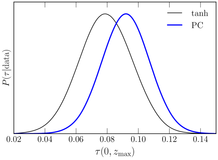
Interestingly, the standard tanh model is moderately disfavored in the wider, observationally complete, PC space leading to changes in the inference for the optical depth summarized in Table 2. In Fig. 5, we compare the posterior probability distributions for the total between the two chains. In the PC analysis the total optical depth constraints shift up by almost 1 from the tanh analysis while having comparable widths. In CDM the main consequence is that the amplitude of structure at goes from in the tanh model to in the PC analysis.
These changes are related to the fact that the standard tanh models only skirt just inside the 2D 95% CL even near the maximum likelihood found in the chain (see Fig. 4). The tanh ML model have the following parameters: , , , , and . Projected onto the PC space through Eq. (2), this value of corresponds to the parameter vector
| (11) |
Note that for the single best constrained component , the tanh ML model is more than off the mean.
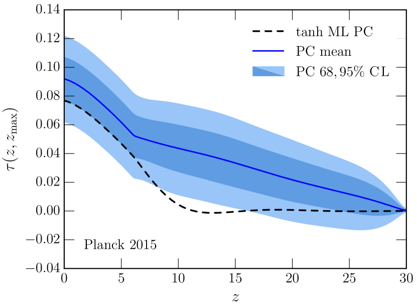
In Fig. 6, we explore the physical origin of this difference. Here we show the and CL constraints on the cumulative optical depth as a parameter derived from the posterior probability. The shape for is fixed by assumption. Note that at , the cumulative optical depth from Eq. (3) becomes approximately
| (12) |
where parametrizes the sum over all of the nonrelativistic density components. Integrals over redshift in Eq. (3) can be precomputed for individual PCs once and for all in a fiducial cosmology as in Fig. 2 and then just summed with weights and a rescaled prefactor following Eq. (12).
At the CL, the data favor optical depth contributions at . For comparison, we also plot the ML tanh model, projected onto the PC basis and calculated in the same way. This model has essentially no optical depth contributions for , not because the data forbid it but because of the functional form of the model. More generally, because of its steplike form, the tanh family of models cannot generate high redshift optical depth without also overproducing the total optical depth (see Table 2).
Given these differences, we explore further their origin in the data. Constraints on the optical depth are also affected by the temperature power spectrum indirectly and directly. Gravitational lens effects place constraints on the amplitude of the matter power spectrum through and so in combination with measurements of the temperature power spectrum which determine constrain indirectly Hu (2002). In particular, the Planck temperature power spectrum favors more gravitational lensing than is predicted by the best fit CDM parameters and hence tends to drive to larger values Ade et al. (2015).
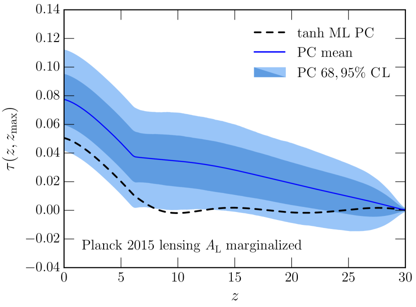
To test whether the preference for high redshift optical depth originates from gravitational lensing and not large angle polarization, we follow the Planck 2015 analysis and marginalize a multiplicative renormalization of the lens power spectrum by adding it to the parameter set of a new MCMC analysis of both the PC and the tanh model. In the PC case we obtain and in the tanh case In Fig. 7, we show the impact on . As expected the total optical depth is approximately 1 lower but notably the high redshift preference weakens only moderately. A finite is still favored at nearly the 95% CL (see also Table 2). We conclude that much of the preference for high vs. low redshift optical depth comes from the large angle polarization data itself.
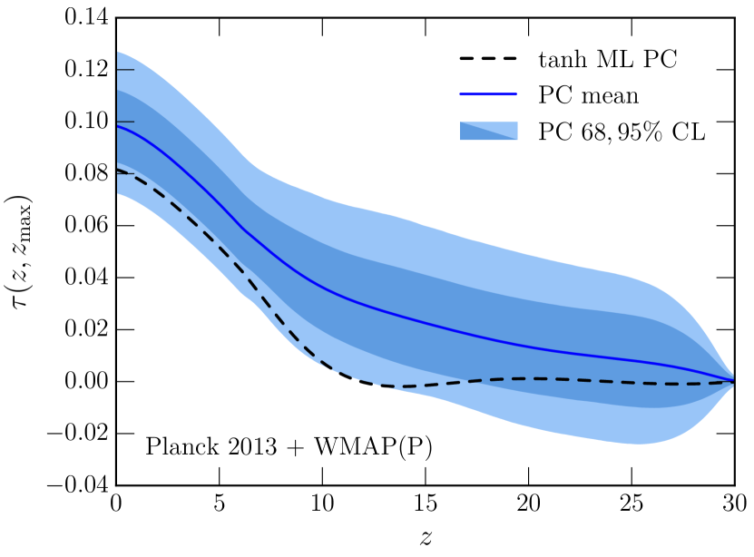
To further test this conclusion, we replace the Planck polarization data with WMAP9. In order to consistently analyze WMAP9 and Planck data sets with publicly available likelihood codes, we also employ Planck 2013 instead of 2015 data. Figure 8 shows that this replacement has a larger impact on the high redshift end with the preference for dropping to almost (see also Table 2). Conversely, the constraints on remain largely the same as the baseline Planck 2015 analysis indicating that they are constrained mainly by the temperature data. As noted in Ref. Mortonson and Hu (2008c) the Doppler effect from reionization imprints features on the temperature spectrum which constrain the higher order PCs. With the extended reach of the Planck temperature power spectrum as compared with WMAP5, these features can be better separated from cosmological parameters.
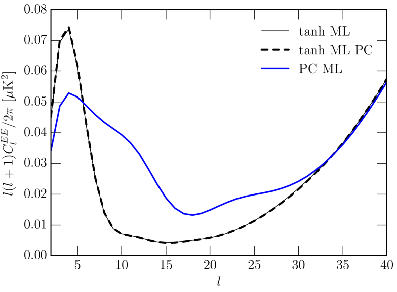
Since the preference for high redshift ionization mainly originates from the low multipole polarization data, it is interesting to compare for the maximum likelihood tanh model from Eq. (11) to the maximum likelihood PC parameters. The PC chain maximum has , , , , and
| (13) |
Note that in both cases the ML is simply the maximum found in the chain samples, not the true maximum in the parameter space. Nonetheless, the difference in likelihood of these two chain maximum models is showing that the preference is not just an artifact of parameter volume and priors.
In Fig. 9 we show that the difference in is that the PC ML has a much broader reionization bump that extends to higher multipoles. This directly corresponds to the preference for high redshift ionization since the angular scale of the feature is determined by the horizon at the redshift of scattering (see Hu and Holder (2003), Fig. 2). In the tanh family of models, tight constraints at require low power between regardless of whether the data prefers it.
We also show in Fig. 9 that the projection of the tanh ML onto the 5 PC basis accurately captures the reionization feature in the polarization spectrum with deviation of for which tests the completeness of the 5 PC basis. In fact most of the deviation is at where the tanh model has minimal power so that the fractional accuracy still reflects a high absolute accuracy.
| Model | Data | ||
|---|---|---|---|
| PC | P15 | 0.092 0.015 | 0.033 0.016 |
| tanh | P15 | 0.079 0.017 | … |
| PC | P15 | 0.078 0.018 | 0.028 0.016 |
| tanh | P15 | 0.056 0.020 | … |
| PC | P13+WMAP(P) | 0.098 0.014 | 0.022 0.018 |
| tanh | P13+WMAP(P) | 0.090 0.013 | … |
IV Ionization History Likelihood
One of the main benefits of our PC reionization analysis is that it completely encapsulates the information from the large angle polarization measurements on the ionization history within the given redshift range. With this single analysis, it is possible to infer constraints on any given reionization model in the same range. In this section, we provide a concrete prescription for an effective likelihood function for the data given an model.
The MCMC PC analysis of the previous section returns the posterior probability density in the space of PC amplitudes given the data and flat priors on the parameters, marginalized over cosmological parameters. Invoking Bayes’ theorem, we can reinterpret it as an effective likelihood of the data given . To determine the likelihood given instead, we simply need to project it onto the PC basis using Eq. (2).
In practice, the MCMC only provides a sample of the PC posterior, represented by discrete elements in the chain with parameter values and multiplicities , whereas a given model produces a continuum of values for . Given the samples, we approximate the effective likelihood with a kernel density estimator of the form
| (14) |
where is the total number of elements in the chain and the overall normalization is arbitrary. Here is a smoothing kernel that makes the function estimate continuous at the expense of artificially broadening the distribution. We choose the shape of to be a multivariate Gaussian of zero mean and covariance where is the covariance matrix estimated from the chain from Table 1 and Eq. (10). For a Gaussian posterior, the effect of smoothing is to increase the covariance by or the errors by approximately . To minimize the amount of smoothing required to capture the behavior of models in the tail of the distribution like the standard tanh model, we oversample the posterior by running the chain past normal convergence requirements for a total of chain elements. In practice we choose . Note also that we employ the full chain without physicality priors since the smoothing kernel transfers information across these boundaries.
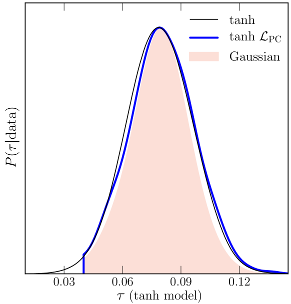
To illustrate and test this approach, we use the effective likelihood to compare constraints on the standard tanh model. In this case the model parameter is the total given the tanh ionization history . We can then construct the posterior probability of as usual via Bayes’ theorem and the effective likelihood given
| (15) |
To match the MCMC analysis of the standard tanh model we take flat priors . For the conversion between the ionization history and we take the cosmological parameters of the ML tanh model.
In Fig. 10, we compare the posterior probabilities from the direct MCMC analysis and the effective PC likelihood. The distributions match to much better than in their means and widths. This is a fairly stringent test on the method given that tanh models live in the tails of the PC posterior. The cutoff at low in the effective likelihood method simply reflects the restriction for the PCs which assumes hydrogen ionization occurred at as is observationally the case.
It is also interesting to compare these results to an even simpler effective likelihood. In Fig. 10 (shaded region), we also show the result of approximating the posterior as a multivariate Gaussian with mean and covariance
| (16) |
For an extremely fast but approximate effective likelihood and for models near the peak of the distribution, the Gaussian approximation may suffice.
Validated on the tanh model, our effective likelihood technique allows a rapid exploration of other models without the need for a separate MCMC analysis. To illustrate this usage, we consider the power-law (PL) models that the Planck Collaboration also analyzed for the HFI data Adam et al. (2016). The PL model
| (17) |
allows for an extended and asymmetric ionization history unlike the tanh model. Here is a parameter that truncates reionization at but has little effect at lower redshift. In order to mimic the analysis in Ref Adam et al. (2016) but allow for the weaker constraints from Planck 2015, we fix so that it does not significantly impact the analysis. The power-law index controls the duration of reionization defined so that . It is therefore more convenient to parametrize the model with and . We employ the effective PC likelihood approach with flat priors for this two parameter family within their allowed ranges.
In Fig. 11, we show the 2D posteriors in these parameters. The Planck 2015 data do indeed allow an extended period of reionization if but do not particularly favor it over a prompt reionization that maintains the same total optical depth. Like the tanh model, the PL model links the low redshift and high redshift ionization history by assumption of a functional form appropriate for models with a single phase of reionization. One should therefore not equate a constraint on the duration of reionization in the PL model with a constraint on high redshift ionization in a more general context. To see this more quantitatively, in Fig. 12 we show the cumulative optical depth constraints in the PL context. The PL models allow very little optical depth at compared with the mean in the full PC space from Fig. 6.
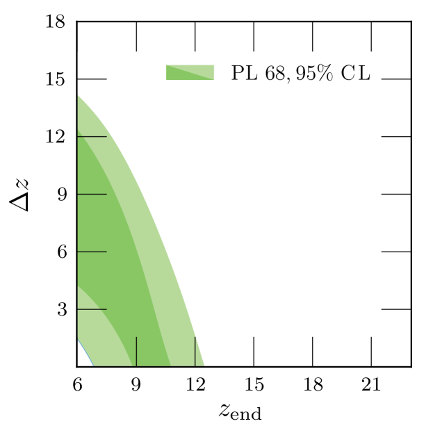
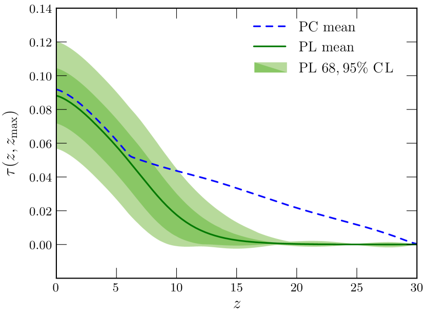
The PL example also illustrates the fact that to encompass the region favored by the PC effective likelihood, a reionization model would need to have an additional source of high redshift ionization that is not directly linked in functional form to its low redshift behavior. We explore such cases in a separate work Miranda et al. (2016). In fact, we also expect the effective likelihood method to work even better for models that are favored by the data since the underlying MCMC sample better represents these models.
V Discussion
By analyzing the Planck 2015 data with an observationally complete PC basis for the ionization history, we show that it allows and even favors high redshift, , optical depth at the level. The standard analysis which includes just the total optical depth and assumes a sharp steplike transition excludes this possibility by prior assumption of form rather than because it is required by the data. The same is true for power-law models that additionally vary the duration of reionization.
While a result amongst the 5 PC parameters is not on its own surprising, it originates from the first and best constrained component and hence has consequences for the total optical depth. The total optical depth is important for understanding a host of other cosmological parameters from the amplitude of the current matter power spectrum to the inferences from CMB lensing. At the very least, this analysis highlights the need for a complete treatment of CMB reionization observables to guarantee a robust interpretation of the optical depth.
This preference for extra high redshift optical depth mainly originates from the large angle polarization spectrum in the Planck 2015 data and appears related to excess power in the multipole range . It is only slightly weakened by marginalizing gravitational lensing information in the temperature power spectrum, which is known to favor a higher optical depth, but more significantly changed by replacing the Planck LFI with WMAP9 polarization data.
While excess polarization power in this range favors additional sources of high redshift ionization such as population III stars or dark matter annihilation it could also indicate contamination from systematics and foregrounds. The latter have been significantly improved in the as yet proprietary Planck 2016 intermediate results. These results indicate that the low redshift end of the optical depth as tested by steplike models, or equivalently the low polarization power, is both better measured and lower than the central value in the Planck 2015 data Aghanim et al. (2016). On the other hand, these results exacerbate the tension with gravitational lensing in the shape of the temperature power spectrum which probes the total optical depth. It will be interesting to see if this complete analysis still prefers an additional high redshift component in the final Planck release.
Regardless of the outcome of resolving the mild tension between steplike reionization scenarios and the Planck 2015 data, the complete PC approach developed here is useful because with a single analysis one can infer constraints on the parameters of any reionization model within the specified redshift range, here , but easily extensible to any desired range. What has presented an obstacle for this approach in the past is the lack of tools for converting posterior parameter constraints on the PCs to parameter constraints on models and so be able to combine them with other sources of reionization information. For example, the ionization history can also be tested in the CMB through the kinetic Sunyaev-Zel’dovich effect from temperature fluctuations beyond the damping scale, but in a manner that is highly model dependent (e.g. Mortonson and Hu (2010); Zahn et al. (2012); Battaglia et al. (2013); Adam et al. (2016)).
Towards this end, we have developed and tested an effective likelihood code for inferring constraints on any given ionization history provided by a model. This approach should be especially useful in constraining models where small high redshift contributions to the optical depth need to be separated from the total.
Acknowledgments: We thank Austin Joyce, Adam Lidz, and Pavel Motloch for useful discussions. W.H. thanks the Aspen Center for Physics, which is supported by National Science Foundation Grant PHY-1066293, where part of this work was completed. C.H. and W.H. were supported by NASA ATP NNX15AK22G, U.S. Dept. of Energy Contract No. DE-FG02-13ER41958, and the Kavli Institute for Cosmological Physics at the University of Chicago through Grants No. NSF PHY-0114422 and No. NSF PHY-0551142. Computing resources were provided by the University of Chicago Research Computing Center. V.M. was supported in part by the Charles E. Kaufman Foundation, a supporting organization of the Pittsburgh Foundation.
References
- Mesinger (2016) A. Mesinger, ed., Understanding the Epoch of Cosmic Reionization: Challenges and Progress, Astrophysics and Space Science Library, Vol. 423 (2016).
- Hu and Jain (2004) W. Hu and B. Jain, Phys. Rev. D70, 043009 (2004), arXiv:astro-ph/0312395 [astro-ph] .
- Smith et al. (2006) K. M. Smith, W. Hu, and M. Kaplinghat, Phys. Rev. D74, 123002 (2006), arXiv:astro-ph/0607315 [astro-ph] .
- Allison et al. (2015) R. Allison, P. Caucal, E. Calabrese, J. Dunkley, and T. Louis, Phys. Rev. D92, 123535 (2015), arXiv:1509.07471 [astro-ph.CO] .
- Mortonson and Hu (2009) M. J. Mortonson and W. Hu, Phys. Rev. D80, 027301 (2009), arXiv:0906.3016 [astro-ph.CO] .
- Mortonson et al. (2009) M. J. Mortonson, C. Dvorkin, H. V. Peiris, and W. Hu, Phys. Rev. D79, 103519 (2009), arXiv:0903.4920 [astro-ph.CO] .
- Mortonson and Hu (2008a) M. J. Mortonson and W. Hu, Phys. Rev. D77, 043506 (2008a), arXiv:0710.4162 [astro-ph] .
- Kogut et al. (2003) A. Kogut et al. (WMAP), Astrophys. J. Suppl. 148, 161 (2003), arXiv:astro-ph/0302213 [astro-ph] .
- Aghanim et al. (2016) N. Aghanim et al. (Planck), (2016), arXiv:1605.02985 [astro-ph.CO] .
- Adam et al. (2016) R. Adam et al. (Planck), (2016), arXiv:1605.03507 [astro-ph.CO] .
- Ahn et al. (2012) K. Ahn, I. T. Iliev, P. R. Shapiro, G. Mellema, J. Koda, and Y. Mao, Astrophys. J. Lett. 756, L16 (2012), arXiv:1206.5007 .
- Hu and Holder (2003) W. Hu and G. P. Holder, Phys. Rev. D68, 023001 (2003), arXiv:astro-ph/0303400 [astro-ph] .
- Lewis et al. (2006) A. Lewis, J. Weller, and R. Battye, Mon. Not. Roy. Astron. Soc. 373, 561 (2006), arXiv:astro-ph/0606552 [astro-ph] .
- Mortonson and Hu (2008b) M. J. Mortonson and W. Hu, Astrophys. J. 672, 737 (2008b), arXiv:0705.1132 [astro-ph] .
- Mortonson and Hu (2008c) M. J. Mortonson and W. Hu, Astrophys. J. 686, L53 (2008c), arXiv:0804.2631 [astro-ph] .
- Ade et al. (2014) P. A. R. Ade et al. (Planck), Astron. Astrophys. 571, A22 (2014), arXiv:1303.5082 [astro-ph.CO] .
- Dai et al. (2015) W.-M. Dai, Z.-K. Guo, and R.-G. Cai, Phys. Rev. D92, 123521 (2015), arXiv:1509.01501 [astro-ph.CO] .
- Becker et al. (2015) G. D. Becker, J. S. Bolton, and A. Lidz, Publ. Astron. Soc. Austral. 32, 45 (2015), arXiv:1510.03368 [astro-ph.CO] .
- Lewis et al. (2000) A. Lewis, A. Challinor, and A. Lasenby, Astrophys. J. 538, 473 (2000), arXiv:astro-ph/9911177 [astro-ph] .
- Howlett et al. (2012) C. Howlett, A. Lewis, A. Hall, and A. Challinor, JCAP 1204, 027 (2012), arXiv:1201.3654 [astro-ph.CO] .
- Becker et al. (2011) G. D. Becker, J. S. Bolton, M. G. Haehnelt, and W. L. W. Sargent, Mon. Not. Roy. Astron. Soc. 410, 1096 (2011), arXiv:1008.2622 [astro-ph.CO] .
- Lewis (2013) A. Lewis, Phys. Rev. D87, 103529 (2013), arXiv:1304.4473 [astro-ph.CO] .
- Lewis and Bridle (2002) A. Lewis and S. Bridle, Phys. Rev. D66, 103511 (2002), arXiv:astro-ph/0205436 [astro-ph] .
- Aghanim et al. (2015) N. Aghanim et al. (Planck), Submitted to: Astron. Astrophys. (2015), arXiv:1507.02704 [astro-ph.CO] .
- Hu (2002) W. Hu, Phys. Rev. D65, 023003 (2002), arXiv:astro-ph/0108090 [astro-ph] .
- Ade et al. (2015) P. A. R. Ade et al. (Planck), (2015), arXiv:1502.01589 [astro-ph.CO] .
- Miranda et al. (2016) V. Miranda, A. Lidz, C. H. Heinrich, and W. Hu, (2016), arXiv:1610.00691 [astro-ph.CO] .
- Mortonson and Hu (2010) M. J. Mortonson and W. Hu, Phys. Rev. D81, 067302 (2010), arXiv:1001.4803 [astro-ph.CO] .
- Zahn et al. (2012) O. Zahn et al., Astrophys. J. 756, 65 (2012), arXiv:1111.6386 [astro-ph.CO] .
- Battaglia et al. (2013) N. Battaglia, A. Natarajan, H. Trac, R. Cen, and A. Loeb, Astrophys. J. 776, 83 (2013), arXiv:1211.2832 [astro-ph.CO] .