Network susceptibilities: theory and applications

Abstract

We introduce the concept of network susceptibilities quantifying the response of the collective dynamics of a network to small parameter changes. We distinguish two types of susceptibilities: vertex susceptibilities and edge susceptibilities, measuring the responses due to changes in the properties of units and their interactions, respectively. We derive explicit forms of network susceptibilities for oscillator networks close to steady states and offer example applications for Kuramoto-type phase-oscillator models, power grid models and generic flow models. Focusing on the role of the network topology implies that these ideas can be easily generalized to other types of networks, in particular those characterizing flow, transport, or spreading phenomena. The concept of network susceptibilities is broadly applicable and may straightforwardly be transferred to all settings where networks responses of the collective dynamics to topological changes are essential.

I Introduction

Susceptibility constitutes a key concept in physics, from statistical mechanics to condensed matter theory and experiments. In these fields, susceptibility quantifies the change of a systems’ state, typically measured by order parameters, in response to a change in some external field. In simple settings, susceptibility is well approximated by linear response theory and one global order parameter changes in response. Generally, there can be many order parameters, as for instance the a site-dependent average spin in the theory of magnetism. While ideal solids are organized in the form of perfectly periodic crystals with, e.g., nearest neighbor interactions, many natural and engineered complex systems are organized in networks with a rich variety of their underlying interaction topologies Strogatz (2001); Newman (2010). The susceptibility of such a networked system, i.e. its response to changes in their parameters, is thus essentially determined by their topology. Furthermore, unlike in periodic systems the response depends crucially on the location of the perturbation. Given that there are different types of local properties that may change, it is not yet clear how to appropriately define susceptibilities in a networked system and consequentially what such susceptibilities would tell us about the collective dynamics.

In this article we introduce two types of susceptibilities in network dynamical systems. Focusing on changes to steady state operating points, we first systematically study the impact of small local perturbations of single units and effective interactions in networks. As a key class of network dynamics, we analyze the susceptibilities of oscillator networks describing the dynamics of various natural and man-made systems. We define both vertex susceptibilities and edge susceptibilities to qualitatively and quantitatively distinguish the responses to changes of single unit and single interaction properties, respectively. In particular, we reveal how the interaction topology of the network jointly with the type and location of the perturbation relative to the response location determine the response strength. These susceptibilities are shown to be related to, but not equal to, established measures of network centrality. Several applications, in particular to Kuramoto phase oscillator and power grid networks, are discussed. We specifically identify certain instances of vertex susceptibilities for electric power grid models as power transfer distribution factors known in electric engineering. Network susceptibilities are readily generalizable to all kinds of supply and transport networks as well as network dynamical systems whose dynamics exhibits a standard flow structure.

II Network Susceptibilities

A continuous time network dynamical system can be described by the equations of motion of $N$ variables (the “vertices”)

$$\frac{dx_{i}}{dt} =F_{i}(x_{1},x_{2},\cdots,x_{N};p_{1},p_{2},\cdots,p_{M}),$$ (1)

where $p_{1},p_{2},\ldots,p_{M}$ are tunable. The network interactions (the “edges”) are defined by which variables $x_{j}$ appear in the equation of motion of $x_{i}$. Now we define network susceptibilities in the following.

Definition 1.

Let $\boldsymbol{x^{*}}=(x_{1}^{*},x_{2}^{*},\cdots,x_{N}^{*})$ be a steady state for a network dynamical system defined by (1). Suppose that on applying a small perturbation to one of the network parameters $p_{k}$:

$$p_{k}\to p_{k}+\varepsilon,$$ (2)

the fixed point changes by a certain amount

$$\boldsymbol{x^{*}} \to\boldsymbol{x^{*^{\prime}}}(\varepsilon).$$ (3)

Then the network susceptibility due to parameter $p_{k}$ is defined as

$$\chi_{(p_{k})\to j} =\lim_{\varepsilon\to 0}\frac{x_{j}^{*^{\prime}}(\varepsilon)-x^{*}}{\varepsilon}.$$ (4)

We note that this definition can easily be extended to dynamics with other invariant sets (e.g. limit cycles) instead of fixed points, and also to stochastic dynamics.

III Dynamics of oscillator networks

As a cornerstone example we analyze the susceptibility of a network of coupled oscillators. The celebrated Kuramoto model Kuramoto (1975) characterizes the collective dynamics of a variety of dynamical systems ranging from chemical reactions Kuramoto (1984) and neural networks Sompolinsky et al. (1990) to coupled Josephson junctions Wiesenfeld et al. (1996), laser arrays Vladimirov et al. (2003) and optomechanical systems Heinrich et al. (2011). In the Kuramoto model, $N$ phase oscillators are coupled via their phase differences. The rate of change of each phase $\phi_{j}$ is given by

$$\frac{d\phi_{j}}{dt}=\omega_{j}+\sum_{\ell=1}^{N}K_{j\ell}\sin(\phi_{\ell}-\phi_{j}),$$ (5)

where $\omega_{j}$ is the intrinsic frequency of the $j$th oscillator, $j\in\{1,\ldots,N\}$, and $K_{j\ell}=K_{\ell j}$ denotes the coupling strength of two oscillators $j$ and $\ell$.

A similar model describes the frequency dynamics of complex power grids and has gained a strong interest recently Rohden et al. (2012); Witthaut and Timme (2012); Dörfler et al. (2013); Motter et al. (2013); Rohden et al. (2014); Nishikawa and Motter (2015). The model describes the dynamics of rotating synchronous generators and motors, representing power plants and consumers, respectively. Each machine is characterized by the power it generates ($P_{j}>0$) or consumes ($P_{j}<0$) and rotates with a frequency close to the grid’s reference frequency $\Omega$ of $2\pi\times 50/60$ Hz, such that its phase is written as $\theta_{j}(t)=\Omega t+\phi_{j}(t)$. The dynamics of the phases is given by the swing equation Machowski et al. (2008); Filatrella et al. (2008)

$$M_{j}\frac{d^{2}\phi_{j}}{dt^{2}}+D_{j}\frac{d\phi_{j}}{dt}=P_{j}+\sum_{\ell=1}^{N}K_{j\ell}\sin(\phi_{\ell}-\phi_{j}),$$ (6)

where $M_{j}$ is proportional to the moment of inertia and $D_{j}$ is proportional to the damping torque of the respective synchronous machine. This ‘oscillator model’ assumes that all consumers can be described as synchronous motors with a non-vanishing inertia $M_{j}$ (It should be noted that since the oscillator model is valid only for the high voltage transmission grid, the consumers do not represent individual electrical devices in each household, but rather whole cities or neighborhoods). In the ‘structure-preserving model’ used in electric power engineering Bergen and Hill (1981) one assumes different consumers. In contrast to a synchronous machine this type of consumer cannot store any kinetic energy, such that the inertia vanishes. Hence, the equations of motion of the structure-preserving model are still given by (6), but with $M_{j}=0$. In the oscillator model as well as the structure-preserving model the power flow from machine $k$ to machine $j$ is given by

$$F_{jk}=K_{jk}\sin(\phi_{k}-\phi_{j}),$$ (7)

where $K_{jk}$ is the maximum transmission capacity which is proportional to the susceptance of the respective transmission line. The relative load of the transmission line is defined as

$$L_{jk}:=\frac{F_{jk}}{K_{jk}}=\sin(\phi_{k}-\phi_{j}).$$ (8)

The two models admit different forms of synchrony. The Kuramoto model was initially introduced to study the emergence of partial synchronization when the coupling of the oscillators in increased Kuramoto (1975). A power grid must be operated in a state of perfect synchronization: All phase differences $\phi_{k}-\phi_{j}$ must be constant in time to enable a steady power flow (7). In this article we analyze how such a phase-locked state responds to a local change in the network, and in particular how this change depends on the topology of the network.

Transforming to a co-rotating frame, the phase-locked states are then just the steady states of Eq. (5) or Eq. (6), respectively, which are determined by the algebraic equation

$$0=P_{j}+\sum_{\ell=1}^{N}K_{j\ell}\sin(\phi_{\ell}-\phi_{j}),$$ (9)

such that we can treat the Kuramoto model and the power grid model on the same footing. However, the perspective of a flow network is particularly helpful in understanding the mathematical results introduced below. We note that the steady states do not depend on the mechanical properties of the individual machines, i.e. the moments of inertia $M_{j}$ and the damping coefficients $D_{j}$.

IV Linear response theory and network susceptibilities

In a complex network there are two general scenarios for a microscopic change of the dynamical system: (1) the modification of an edge weight (signifying e.g. a electrical transmission line capacity) or (2) the modification of a vertex property (e.g. the power generation of a power plant) of the system. In the following, we introduce a linear response theory for both scenarios.

IV.1 Perturbation at a single edge

In the first scenario we consider the coupling matrix $K_{ij}$ being perturbed slightly to yield the new perturbed matrix $K_{ij}^{\prime}$, which differs from $K_{ij}$ only at a single edge $(s,t)$:

$$K^{\prime}_{ij} = K_{ij}+\kappa_{ij}$$ (10)

$$\kappa_{ij} = \left\{\begin{array}[]{l c l}\kappa&\;\mbox{ for }&(i,j)=(s,t)\,\mbox{and}\,(i,j)=(t,s)\\ 0&&\mbox{all other edges.}\\ \end{array}\right.$$ (13)

This perturbation causes the steady state phases of the network to change from $\phi_{j}$ to $\phi^{\prime}_{j}$. The new steady state equation (9) now reads

$$\quad 0 = P_{j}+\sum_{i=1}^{N}K^{\prime}_{ij}\sin(\phi^{\prime}_{i}-\phi^{\prime}_{j}),$$ (14)

$$\forall j\in\left\{1,\ldots,N\right\}.$$ (15)

In the following we calculate this perturbation within a linear response theory. We note that the steady state is defined only up to a global phase shift. Throughout this article we fix this phase such that $\sum\nolimits_{j}\phi_{j}=0$.

We expand the steady state condition (15) to leading order in $\kappa_{ij}$ and

$$\xi_{j}:=\phi_{j}^{\prime}-\phi_{j},$$ (16)

and subtract (9), to obtain

$$0 = \sum_{i=1}^{N}\kappa_{ij}\sin(\phi_{i}-\phi_{j})+\sum_{i=1}^{N}K_{ij}\cos(\phi_{i}-\phi_{j})(\xi_{i}-\xi_{j})$$ (17)

$$= \kappa L_{st}(\delta_{js}-\delta_{jt})-\sum_{i=1}^{N}A_{ji}\xi_{i}$$

for all $j=1,\ldots,N$ using the Kronecker symbol $\delta$. In the last step we have used the definition of the flow (7), the definition of relative load (8) and the perturbation matrix (13). Furthermore, we have introduced the matrix

$$A_{ij} := \left\{\begin{array}[]{l c l}-\widetilde{K}_{ij}&\;\mbox{for}&i\neq j\\ +\sum_{\ell}\widetilde{K}_{\ell j}&&i=j\\ \end{array}\right.\qquad\mbox{where}$$ (20)

$$\widetilde{K}_{ij} := K_{ij}\cos(\phi_{i}-\phi_{j}).$$ (21)

In a short-hand vectorial notation, Eq. (17) then reads

$$A\boldsymbol{\xi}=\kappa L_{st}\boldsymbol{q}_{(st)},$$ (22)

using the vector $\boldsymbol{q}_{(st)}\in\mathbb{R}^{N}$ with the components

$$\boldsymbol{q}_{(st),j}=(\delta_{s,j}-\delta_{t,j}).$$ (23)

We note that the matrix $A$ is singular such that it cannot be inverted. However, the vector $\boldsymbol{q}$ is orthogonal to the kernel of $A$ which is spanned by the vector $(1,1,\ldots,1)^{t}$ such that this is no problem. In order to formally solve Eq. (22) we can thus use the Moore-Penrose pseudoinverse of $A$, which we will call $T:=A^{+}$ in the following. Thus we find

$$\boldsymbol{\xi}=\kappa L_{st}\;T\boldsymbol{q}_{st}.$$ (24)

The perturbed flow (7) over an edge $(i,j)$ is then given by

$$F^{\prime}_{ij} = (K_{ij}+\kappa_{ij})\sin(\phi_{j}-\phi_{i}+\xi_{j}-\xi_{i})$$ (25)

$$= K_{ij}\sin(\phi_{j}-\phi_{i})+\kappa_{ij}\sin(\phi_{j}-\phi_{i})$$

$$\quad+K_{ij}\cos(\phi_{j}-\phi_{i})(\xi_{j}-\xi_{i})$$

up to first order in $\kappa$ and $\boldsymbol{\xi}$. Using Eq. (24), this result reads

$$F^{\prime}_{ij}=F_{ij}+ \kappa L_{st}\big{[}(\delta_{is}\delta_{jt}-\delta_{js}\delta_{it})$$ (26)

$$+\widetilde{K}_{ij}(T_{js}-T_{jt}-T_{is}+T_{it})\big{]}.$$

IV.2 Edge susceptibilities

Depending on the application we want to measure different effects caused by the perturbation at the edge $(s,t)$. First we quantify how much the phase of a single oscillator $j$ is affected by the edge-to-vertex susceptibility, using (24)

$$\chi_{(st)\rightarrow j} := \lim_{\kappa\rightarrow 0}\frac{\phi_{j}^{\prime}-\phi_{j}}{\kappa}$$ (27)

$$= L_{st}(T_{js}-T_{jt}).$$

To measure the change of the oscillator state on a global scale in response to perturbation at a single edge, we define the global edge susceptibility as the norm of the local susceptibilities

$$\chi_{(st)}^{2} := \lim_{\kappa\rightarrow 0}\frac{\sum_{j}|\phi_{j}^{\prime}-\phi_{j}|^{2}}{\kappa^{2}}$$ (28)

$$= \sum_{j=1}^{N}\chi_{(st)\rightarrow j}^{2}$$

$$= L_{st}^{2}\sum_{j=1}^{N}(T_{js}-T_{jt})^{2}\,.$$

For applications to flow networks, such as the power grid model (6), we are especially interested in how the flows change as this determines the stability of the grid. In particular, stability can be lost when a single edge becomes overloaded. Thus, we define the edge-to-edge susceptibility as the change of flow at another edge

$$\eta_{(st)\rightarrow(ij)}:=\lim_{\kappa\rightarrow 0}\frac{F_{ij}^{\prime}-F_{ij}}{\kappa}\,.$$ (29)

Using Eq. (26) this relation reads

$$\eta_{(st)\rightarrow(ij)}=L_{st}\big{[} (\delta_{is}\delta_{jt}-\delta_{js}\delta_{it})$$ (30)

$$+\widetilde{K}_{ij}(T_{js}-T_{jt}-T_{is}+T_{it})\big{]}.$$

We conclude that the effects of a perturbation at a single edge $(s,t)$ as measured by the susceptibilities defined above are proportional to the load of edge $L_{st}$. Furthermore, the susceptibilities are essentially given by the matrix $T$, the pseudoinverse of $A$. The properties of these matrices will be analyzed in detail in the following sections.

IV.3 Perturbation at a single vertex

The above calculations can be readily generalized to analyze the change of the steady state in response to a local perturbation of a single vertex property. To this end we consider a change of the power injected at a single vertex $s$. However, a steady state of Eq. (6) exists only if the power is balanced such that we consider a small perturbation of the power vector of the form

$$P_{j}^{\prime}=P_{j}+p\,(\delta_{j,s}-1/N).$$ (31)

Expanding the definition of a steady state to leading order in $p$ and $\xi_{j}:=\phi_{j}^{\prime}-\phi_{j}$ then yields

$$0 = p\,(\delta_{j,s}-1/N)+\sum_{i=1}^{N}\widetilde{K}_{ij}(\xi_{i}-\xi_{j})$$ (32)

$$= p\,(\delta_{j,s}-1/N)+\sum_{i=1}^{N}A_{ij}\xi_{i}.$$

Solving this equation for the changes $\boldsymbol{\xi}$ yields

$$\boldsymbol{\xi}=p\;T\boldsymbol{r}_{s}$$ (33)

with the vector $\boldsymbol{r}_{s}\in\mathbb{R}^{N}$ whose components are given by

$$r_{s,j}=\delta_{s,j}\,.$$ (34)

IV.4 Vertex susceptibilities

In analogy to the case of a perturbed edge discussed in section (IV.2) we define the vertex-to-vertex susceptibility as

$$\chi_{s\rightarrow j} := \lim_{p\rightarrow 0}\frac{\phi_{j}^{\prime}-\phi_{j}}{p}$$ (35)

$$= T_{js},\$$

the global vertex susceptibility as

$$\chi_{s}^{2} := \sum_{j=1}^{N}\chi_{s\rightarrow j}^{2}$$ (36)

$$= \sum_{j=1}^{N}T_{js}^{2},$$

and the vertex-to-edge susceptibility as

$$\eta_{s\rightarrow(ij)} := \lim_{p\rightarrow 0}\frac{F_{ij}^{\prime}-F_{ij}}{p}$$ (37)

$$= \widetilde{K}_{ij}(T_{js}-T_{is}).$$

We note that measures similar to the vertex-to-vertex susceptibility $\chi_{s\rightarrow j}$ are used in electric power engineering where they are called power transfer distribution factors Wood et al. (2013); Ronellenfitsch et al. (2016a). In this context one generally uses a fixed reference or slack node which absorbs the power change $p$, such that Eq. (31) is modified to

$$P_{j}^{\prime}=P_{j}+p\,(\delta_{j,s}-\delta_{j,\rm slack}).$$ (38)

IV.5 Properties of the matrix $A$

We have shown that the response of a network to a local perturbation is essentially given by the matrix $T$, which is the Moore-Penrose pseudoinverse of the matrix $A$ defined in Eq. (21). Before we discuss the potential applications of the network susceptibilities we thus have a closer look at the properties of the matrix $A$.

The matrix $A$ encodes the dynamical stability and synchrony of steady states D.Manik, D. Witthaut, B. Schaf̈er, M. Matthiae, A. Sorge, M. Rohden, E. Katifori and M. Timme (2014); Skardal et al. (2014). A steady state of the Kuramoto model or the power grid model defined by Eq. (6) is dynamically stable if and only if $A$ is positive semi-definite, i.e. all its eigenvalues $a_{j},1\leq j\leq N$ are non-negative. For sake of simplicity we fix the ordering of the eigenvalues such that $0=a_{1}\leq a_{2}\leq a_{3}\leq\cdots a_{N}$. We have to take into account that $A$ always has one eigenvalue $a_{1}=0$. The corresponding eigenvector is $(1,1,\cdots,1)$; signifying that a small perturbation that is exactly the same in all phase angles is neutrally stable. However, this is merely due to the steady state itself being arbitrary up to a constant global phase shift. Stable steady states can emerge or disappear when a system parameter is varied through an (inverse) saddle node bifurcation at which one eigenvalue vanishes, $a_{2}\rightarrow 0$.

In particular, $A$ is positive semi-definite if the relation $\cos(\phi_{i}-\phi_{j})>0$ holds for all edges $(i,j)$ of the network and the network is globally connnected. Stable steady states which do not satisfy this relation typically exist only at the edge of the stable parameter region D.Manik, D. Witthaut, B. Schaf̈er, M. Matthiae, A. Sorge, M. Rohden, E. Katifori and M. Timme (2014). We can thus assume that during normal operation we always have $\cos(\phi_{i}-\phi_{j})\geq 0$ for all edges such that we can use the following relations:

$$\cos(\phi_{i}-\phi_{j}) = \sqrt{1-\sin(\phi_{i}-\phi_{j})^{2}}\geq 0$$

$$\Rightarrow\widetilde{K}_{ij}=K_{ij}\cos(\phi_{i}-\phi_{j}) = \sqrt{K_{ij}^{2}-F_{ij}^{2}}.$$ (39)

The expression $\widetilde{K}_{ij}$ can be understood as the free capacity of an edge $(ij)$, which can be used to respond to the perturbation and is thus refereed to as the responsive capacity.

For normal operation, $\cos(\phi_{i}-\phi_{j})\geq 0$ for all edges $(i,j)$, the non-diagonal entries of the matrix $A$ are all non-positive such that $A$ is a Laplacian matrix for which many properties are known Newman (2010). In particular, the eigenvalues of a Laplacian matrix satisfy $0=a_{1}\leq a_{2}\leq\cdots\leq a_{N}$, where $a_{2}$ is an algebraic measure for the connectivity of the underlying network Fiedler (1973); Fortunato (2010).

V Susceptibility and connectivity

V.1 Scaling properties of network susceptibilities

The susceptibilities are especially large in the limit of a weakly connected network. For a power grid this corresponds to the scenario of high loads when the responsive capacities $\widetilde{K}_{ij}$ become small. In the following we analyze this case in detail for a perturbation at a single edge $(s,t)$ (cf. Eq. (13)). The case of a vertex perturbation is discussed briefly at the end of this section.

Figure 1: The global edge susceptibility $\chi_{(st)}$ in a model power grid. (a) Coarse-grained topology of the British high-voltage power transmission grid Simonsen et al. (2008); Rohden et al. (2012). We randomly choose 60 nodes to be generators with $P_{j}=+1$ ($\square$) and 60 nodes to be consumers with $P_{j}=-1$ ($\circ$). The transmission capacity of all edges is given by $K=4$ in arbitrary units. The color map shows the load $|L_{st}|$ of each edge. (b) Color map plot of the global edge susceptibility $\chi_{st}$. (c) For a given network, the susceptibility is approximately proportional to the load of the edge $|L_{st}|$. It is increased if the edge $(s,t)$ couples two weakly connected components of the responsive capacity graph $\widetilde{K}$, indicated by a large overlap with the Fiedler vector $|\boldsymbol{q}_{st}\cdot\boldsymbol{v}_{2}|$ (shown as a color code and in the inset). (d) On a global scale, the average susceptibility is proportional to the inverse algebraic connectivity $1/a_{2}$. The plot shows $1/a_{2}$ ($\square$, right scale) and the ratio $\chi_{st}/|L_{st}|$ averaged over all edges ($\circ$, left scale) as a function of the transmission capacity $K$. The shading shows the standard deviation of $\chi_{st}/|L_{st}|$.

Throughout this section we assume the case of ’normal’ operation, i.e. we assume that $\widetilde{K}_{ij}\geq 0$ for all edges $(i,j)$. Then the matrix $A$ is a Laplacian matrix with eigenvalues $0=a_{1}\leq a_{2}\leq\cdots\leq a_{N}$ and the associated eigenvectors $\boldsymbol{v}_{n}$. We can then formally solve Eq. (22) for $\boldsymbol{\xi}$ with the result

$$\boldsymbol{\xi} = \kappa L_{st}\sum_{n=2}^{N}\frac{1}{a_{n}}(\boldsymbol{v}_{n}\cdot\boldsymbol{q}_{st})\boldsymbol{v}_{n}.$$ (40)

The term $n=1$ does not contribute since we have fixed the global phase such that $\sum\nolimits_{j}\xi_{j}=0$. This expression shows four important properties of the network susceptibility:

(1) The response $\boldsymbol{\xi}$ and thus also the edge susceptibilities scale with the load of the perturbed edge $L_{st}=F_{st}/K_{st}$. For a complete breakdown of an edge $(s,t)$, we have $\kappa=-K_{st}$ such that $\boldsymbol{\xi}$ scales with the flow $F_{st}$ of the defective edge. The scenario of a complete breakdown is further discussed in Sec. VII.

(2) The prefactors $1/a_{n}$ decrease with $n$. In particular for a weakly connected network the algebraic connectivity $a_{2}$ becomes very small Fiedler (1973); Newman (2010); Fortunato (2010), such that the term $n=2$ dominates the sum. Then the susceptibility of all edges in the network scale inversely with the algebraic connectivity $a_{2}$. This proves our claim that the susceptibility is large if the network defined by the responsive capacities $\widetilde{K}_{ij}$ is weakly connected.

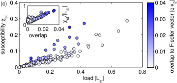
(3) For a weakly connected network, the edge susceptibility scales with the overlap $|\boldsymbol{v}_{2}\cdot\boldsymbol{q}_{st}|$, where $\boldsymbol{v}_{2}$ is the so-called Fiedler vector. This overlap can be interpreted as a measure of the local algebraic connectivity of the nodes $s$ and $t$. To see this note that the Fiedler vector can be used to partition a graph into two weakly connected parts Newman (2010); Fortunato (2010). The overlap with the vector $\boldsymbol{q}_{st}$ is largest if the two nodes $s$ and $t$ are in different parts and thus weakly connected.

(4) In the limit of a disconnected network the response $\boldsymbol{\xi}$ to a perturbation at the edge $(s,t)$ diverges if the edge links the weakly-connected components. If the perturbation occurs within one component, then the response remains finite. This will be shown in detail in the following section.

(5) The global edge susceptibility defined in Eq. (28) can be expressed as

$$\chi_{(st)}^{2}=L_{st}^{2}\sum_{n=2}^{N}\frac{(\boldsymbol{v}_{n}\cdot\boldsymbol{q}_{st})}{a_{n}^{2}},$$ (41)

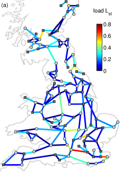
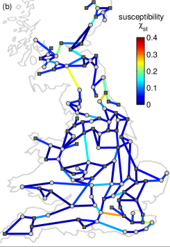
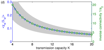
where we have used Eq. (40) for the phase response. This quantity measures the average phase response to the perturbation of a single edge $(s,t)$. An example is shown in Fig. 1 for a synthetic power grid model based on the topology of the British high-voltage grid. One observes that the global susceptibility of an edge $(s,t)$ is essentially determined by the load $L_{st}$, the connectivity of the network and the location of the edge within the network. Edges are highly susceptible if they are heavily loaded or connect two components of the grid. In the shown example we observe two highly susceptible edges connecting the northern part to the rest of the grid. Averaging the global susceptibilities $\chi_{st}$ over all edges $(s,t)$ in the network, we find an almost perfect proportionality with the inverse algebraic connectivity $1/a_{2}$. If the transmission capacity $K$ of the edges increases, the algebraic connectivity $a_{2}$ also increases and the grid becomes less susceptible to perturbations.

V.2 The weakly connected limit

To obtain a more quantitative understanding of the susceptibility in a weakly connected network we assume that the network is decomposed into two components of size $N_{1}$ and $N_{2}=N-N_{1}$, respectively. In the limit of complete disconnection, the Laplacian matrix also decomposes

$$A^{(0)}=\begin{pmatrix}A_{1}^{(0)}&0\\ 0&A_{2}^{(0)}\\ \end{pmatrix}$$ (42)

with $A_{1}^{(0)}\in\mathbb{R}^{N_{1}\times N_{1}}$ and $A_{2}^{(0)}\in\mathbb{R}^{N_{2}\times N_{2}}$. As usual for a Laplacian matrix the lowest eigenvalue vanishes, $a_{1}=0$, and the associated eigenvector is given by

$$\boldsymbol{v}_{1}=\frac{1}{\sqrt{N}}(1,1,\ldots,1)^{T}.$$ (43)

In the disconnected limit also the second eigenvalue (the algebraic connectivity), vanishes, $a_{2}^{(0)}=0$. The associated eigenvector, the Fiedler vector, is given by

$$\boldsymbol{v}_{2}^{(0)}=\frac{1}{\sqrt{N}}\;(\underbrace{\sqrt{N_{2}/N_{1}},\ldots}_{N_{1}\;\mbox{times}}\,,\underbrace{-\sqrt{N_{1}/N_{2}},\ldots}_{N_{2}\;\mbox{times}})^{T}.$$ (44)

Here and in the following the superscript $(0)$ denotes the limiting case of a complete disconnection of the network. For simplicity we assume that the two components are not further disconnected such that $a_{3}^{(0)}>0$.

To analyze the case of a weakly-connected network, we consider a single weak link at position $(c,d)$ between the two components. The Laplacian is then given by $A=A^{(0)}+A^{\prime}$ with

$$A^{\prime}_{cd}=A^{\prime}_{dc}=-k$$

$$A^{\prime}_{cc}=A^{\prime}_{dd}=+k$$ (45)

and $A^{\prime}_{ij}=0$ otherwise. The connection strength $k$ of the edge $(c,d)$ is assumed to be small such that we can calculate the eigenvalues and eigenvectors using Rayleigh-Schrödinger perturbation theory (see, e.g., Ballentine (1998)). We then find the algebraic connectivity

$$a_{2}=k\frac{N_{1}+N_{2}}{N_{1}N_{2}}+\mathcal{O}(k^{2})$$ (46)

and the Fiedler vector

$$\boldsymbol{v}_{2}=\boldsymbol{v}_{2}^{(0)}+k\sqrt{\frac{N_{1}+N_{2}}{N_{1}N_{2}}}\sum_{n=3}^{N}\frac{(\boldsymbol{v}_{n}^{(0)}\cdot\boldsymbol{q}_{cd})}{a_{n}^{(0)}}\boldsymbol{v}_{n}^{(0)}+\mathcal{O}(k^{2}),$$ (47)

where $\boldsymbol{q}_{cd}$ is defined as in Eq. (23).

To calculate the response of the network $\boldsymbol{\xi}$ we need the overlap of the vector $\boldsymbol{q}_{st}$ (see Eq. (40)) with the eigenvectors of $A$, in particular the overlap with the Fiedler vector. The result depends crucially on the location of the perturbed edge $(s,t)$. If this edge connects the two components, i.e. $(s,t)=(c,d)$, we find

$$\boldsymbol{v}_{2}\cdot\boldsymbol{q}_{st}=\sqrt{\frac{N_{1}+N_{2}}{N_{1}N_{2}}}+\mathcal{O}(k)$$ (48)

such that the response diverges as $k^{-1}$:

$$\boldsymbol{\xi}=\frac{\kappa L_{st}}{k}\sqrt{\frac{N_{1}N_{2}}{N_{1}+N_{2}}}\boldsymbol{v}_{2}^{(0)}+\mathcal{O}(k^{0}).$$ (49)

If the edge $(s,t)$ lies within one component, then

$$\boldsymbol{v}_{2}\cdot\boldsymbol{q}_{s,t}=k\sqrt{\frac{N_{1}+N_{2}}{N_{1}N_{2}}}\sum_{n=3}^{N}\frac{(\boldsymbol{v}_{n}^{(0)}\cdot\boldsymbol{q}_{cd})(\boldsymbol{v}_{n}^{(0)}\cdot\boldsymbol{q}_{st})}{a_{n}^{(0)}}+\mathcal{O}(k^{2})$$

such that the response remains finite in the limit $k\rightarrow 0$:

$$\boldsymbol{\xi} = \kappa L_{st}\sqrt{\frac{N_{1}N_{2}}{N_{1}+N_{2}}}\sum_{n=3}^{N}\frac{(\boldsymbol{v}_{n}^{(0)}\cdot\boldsymbol{q}_{cd})(\boldsymbol{v}_{n}^{(0)}\cdot\boldsymbol{q}_{st})}{a_{n}^{(0)}}\boldsymbol{v}_{2}^{(0)}$$ (50)

$$+\kappa L_{st}\sum_{n=3}^{N}\frac{(\boldsymbol{v}_{n}^{(0)}\cdot\boldsymbol{q}_{st})}{a_{n}^{(0)}}\boldsymbol{v}_{n}^{(0)}.$$

For a perturbation at a single vertex as defined in Eq. (31) the response will always diverge in the limit $k\rightarrow 0$. Assuming w.l.o.g. that the perturbed vertex $s$ is an element of the component $1$ we find that

$$\boldsymbol{\xi}=\frac{p}{k}\,\frac{N^{2}}{N_{1}N_{2}}(\underbrace{N_{2}/N_{1},\ldots,N_{2}/N_{1}}_{N_{1}\;\mbox{times}}\,,\underbrace{-1,\ldots,-1}_{N_{2}\;\mbox{times}})^{T}\,$$ (51)

to leading order.

VI Applications

VI.1 The relation to centralities

Various centrality measures have been defined to quantify the importance of single vertices and edges in complex networksNewman (2005). Centrality measures based on current flows Brandes and Fleischer (2005) are heavily used in different areas of network science and are directly related to susceptibility measures as defined in the present article. To illustrate this, consider a network of ohmic resistors with conductances $G_{ij}$. An electrical current flows through the network with $I^{\rm source}_{j}$ being the current in- or outflow at vertex $j$. The current through a particular edge $(i,j)$ of the network is given by the voltage drop across the edge such that

$$I_{ji}=G_{ji}(V_{j}-V_{i}).$$ (52)

At each vertex the current is conserved such that Kirchhoff’s law

$$\sum_{i=1}^{N}I_{ji}=\sum_{i=1}^{N}G_{ji}(V_{j}-V_{i})=I^{\rm source}_{j}$$ (53)

is satisfied for all $j=1,\ldots,N$. Defining the Laplacian matrix of the conductances (the so called nodal conductance matrix)

$$A_{ij} := \left\{\begin{array}[]{l c l}-G_{ij}&\;\mbox{for}&i\neq j\\ +\sum_{\ell}G_{\ell j}&&i=j\\ \end{array}\right.$$ (56)

and its Moore-Penrose pseudoinverse $T:=A^{+}$, the voltages are given by

$$\boldsymbol{V}=T\boldsymbol{I}^{\rm source}.$$ (57)

For the definition of centrality measures Newman (2005) one considers the situation that a unit current flows into the network at a single vertex $s$ and out at a different vertex $t$. Then we have the voltages

$$V_{j}=T_{js}-T_{jt}$$ (58)

and the current flowing over the edge $(i,j)$ is given by

$$I_{ji}=G_{ji}(T_{js}-T_{jt}-T_{is}+T_{it}).$$ (59)

The current flow betweenness centrality of an edge $(i,j)$ is then defined as the absolute current flowing through the edge averaging over all scenarios of the in-/out-flow, i.e. all pairs $(s,t)$ Newman (2005)

$$b_{(i,j)}:=\frac{2}{N(N-1)}\sum_{s<t}G_{ji}|T_{js}-T_{jt}-T_{is}+T_{it}|.$$ (60)

Correspondingly, the betweenness centrality of a vertex $j$ is defined as

$$b_{j} := \frac{1}{N(N-1)}\sum_{s<t}\sum_{i=1}^{N}G_{ji}|T_{js}-T_{jt}-T_{is}+T_{it}|$$ (61)

$$= \sum_{i=1}^{N}\frac{1}{2}\,b_{(i,j)}.$$

We directly see the analogies to the definition of the network susceptibilities if we identify the conductance $G_{ij}$ with the responsive capacity $\widetilde{K}_{ij}$. In particular, the edge betweenness centrality defined in Eq. (60) coincides with the average of the normalized edge-to-edge susceptibility $\eta_{st\rightarrow ij}/|L_{s,t}|$ except for a slight difference in the term $(s,t)=(i,j)$ that vanishes as $1/N^{2}$.

However, in this article we generalize the idea of centralities based on current flow in several ways. First of all, we consider two different scenarios for the in- and outflow of the network: First, for the edge susceptibilities we consider an inflow at vertex $s$ and outflow at vertex $t$ with strength $L_{st}$ as in Newman (2005)

$$I^{\rm source}_{j}=L_{st}(\delta_{js}-\delta_{st}).$$ (62)

Second, for the vertex susceptibilities we assume a unit inflow at vertex $s$ and equal outflow at all other vertices such that

$$I^{\rm source}_{j}=\delta_{js}-\frac{1}{N}\,.$$ (63)

Third, we analyze not only the change of the flows as in the edge-to-edge susceptibilities, but also the change of the state variables $\xi_{j}$ which correspond to the voltages in the resistor networks. In this sense, the global susceptibilities $\chi^{2}_{(st)}$ and $\chi^{2}_{s}$ are given by the variance of the voltages in the network. Therefore they quantify the global response of the network to a local in- or outflow in terms of the average variation of all voltages.

VI.2 Relation to resistance distances

In a manner similar to the previous section VI.1, the concept of susceptibilities can be understood in terms of resistance distance, which is defined as follows. As in the previous section we consider a network of Ohmic resistors with conductances $G_{ij}$ and suppose a unit current enters the node $s$ and exits through node $t$. Then the resistance distance $R_{st}$ is given by the voltage drop between the nodes $s$ and $t$. Using the relation (58), this yields

$$R_{st}=V_{s}-V_{t}=T_{ss}-2T_{st}+T_{tt}.$$ (64)

using the symmetry of the matrix $T$. This relation can be inverted with the result Palacios (2001)

$$T_{ij} =-\frac{1}{2}R_{ij}+\frac{1}{2N}\left(R_{j}^{\rm tot}+R_{i}^{\rm tot}\right)-\frac{\sum_{i,j}R_{ij}}{N^{2}}$$ (65)

where we have defined $R_{i}^{\rm tot}=\sum_{j}R_{ij}$.

Substituting Eq. (65) into (24) and (35), we can express all susceptibilities equivalently in terms of the matrix $T$ or the resistance distances. For the vertex-to-vertex susceptibility we find

$$\chi_{s\rightarrow t} =-\frac{1}{2}R_{st}+\frac{1}{2N}R_{s}^{\rm tot}+\frac{1}{2N}R_{t}^{\rm tot},$$ (66)

and subsequently the global average of susceptibilities take the simple form

$$\sum_{t\neq s}\chi_{s\rightarrow t} =\frac{1}{2}\sum_{i,j}G_{ij}-\frac{1}{N}R_{s}^{\rm tot}.$$ (67)

This relation clearly demonstrates that nodes that are on an average “close" to the rest of the network (i.e. with high centrality values), tend to have higher global susceptibility.

In a similar manner, the vertex-to-edge susceptibilities can be expressed as

$$\eta_{s\to(i,j)} =\widetilde{K}_{ij}\left\{-\frac{1}{2}(R_{si}-R_{sj})+\frac{1}{2N}(R_{i}^{\rm tot}-R_{j}^{\rm tot})\right\}$$ (68)

and the edge-to-vertex susceptibility follows an almost identical form, apart from the prefactor:

$$\eta_{(i,j)\to s} =L_{ij}\left\{-\frac{1}{2}(R_{si}-R_{sj})+\frac{1}{2N}(R_{i}^{\rm tot}-R_{j}^{\rm tot})\right\}.$$ (69)

The global edge susceptibilities are given by (derivation in Appendix A):

$$\chi^{2}_{(ij)}=$$ (70)

$$\;\frac{NL_{st}^{2}}{4}\left(\frac{1}{N}\sum_{s}(R_{si}-R_{sj})^{2}-\left[\frac{1}{N}\sum_{s}(R_{si}-R_{sj})\right]^{2}\right).$$

VI.3 Scaling with distance

Figure 2: The Vertex-to-vertex susceptibility in uniform and realistic network topologies. (a) Color coded plot of $\chi_{s\rightarrow t}$ in a $256\times 256$ square grid with uniform free capacities, showing logarithmic decay. The central vertex $s$ was perturbed. (b) Decay behavior of the mean $\chi_{s\rightarrow t}$ in the same topology as in (a) as a function of shortest path distance $d(s,t)$. The shaded region represents a 95% confidence interval. We clearly see logarithmic decay. (c) Color coded plot of $\chi_{s\rightarrow t}$ in the Continental European Transmission Network topology with realistic free capacities (taken from Hutcheon and Bialek (2013)). The vertex positions are not realistic. One central vertex was perturbed. There are several highly susceptible vertices in the network periphery (dark blue). (d) Decay behavior of the mean $\chi_{s\rightarrow t}$ in the same topology as in (c) as a function of $d(s,t)$. We show both realistic free capacities $\tilde{K}_{ij,\mathrm{real}}$ as well as uniform free capacities $\tilde{K}_{ij,\mathrm{unif}}=\langle\tilde{K}_{\mathrm{real}}\rangle$ set to the mean realistic value. The same vertex as in (c) was perturbed. In the realistic case, few highly susceptible vertices in the network periphery lead to a high variance at large distances, in contrast to the uniform case.

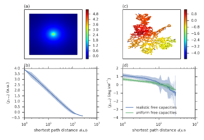
The effect of a linear perturbation generally decays with distance. To obtain a better understanding of this decay, we consider a continuum version of the linear response theory, concentrating on the vertex-to-vertex susceptibility. We consider a two-dimensional square lattice with equal weights, as power grids are naturally embedded into a two-dimensional plane and most grids can can be assumed to be approximately planar. In the continuum limit the Laplacian matrix tends to the two-dimensional Laplace operator and Eq. (32) becomes a Poisson equation,

$$\Delta\xi(\boldsymbol{x})=p\delta(\boldsymbol{x}-\boldsymbol{x}_{0}),$$ (71)

where $\xi(\boldsymbol{x})$ is the local response at position $\boldsymbol{x}$ (e.g. the local phase angle), $p$ is the power injection which occurs at position $\boldsymbol{x}_{0}$ and $\Delta$ is the 2D Laplace operator. The solutions to this equation are well known. On an infinite two-dimensional domain it is

$$\xi(\boldsymbol{x})=\frac{p}{2\pi}\log(|\boldsymbol{x}-\boldsymbol{x}_{0}|)+b,$$ (72)

where $b$ is a constant of integration. Generally, no unique notion of Euclidean distance between nodes exists for networks. The closest analog is the shortest path distance, denoted by $d(s,t)$ in the following, which is related to the Euclidean distance for instance in regular grids. Figure 2 (a, b) show the decay behavior in a uniform square grid, compatible with the continuum results.

Realistic network topologies are more complicated as shown in Fig. 2 (c, d). We computed the susceptibility of the Continental European Transmission Network Hutcheon and Bialek (2013) to perturbing one vertex for two cases of free capacities $\tilde{K}$. First, we obtained realistic values $\tilde{K}_{ij,\mathrm{real}}$ from Hutcheon and Bialek (2013), then we considered a uniform model in which all free capacities are replaced by the average $\tilde{K}_{ij,\mathrm{unif}}=\langle\tilde{K}_{\mathrm{real}}\rangle$. In the vicinity of the perturbation, monotonic decay can be seen in both cases. However, there exist several vertices in the periphery of the network that are much more susceptible than the rest for realistic free capacities (dark blue in Fig. 2 (c)). These vertices are highly susceptible independent of the perturbed vertex.

Figure 3: The edge-to-vertex susceptibility in uniform and realistic network topologies. (a) Color coded plot of $\chi_{(s,t)\rightarrow j}$ in a $256\times 256$ square grid with uniform free capacities. The central edge ((128,128), (128,129)), where the numbers are integer coordinates, was perturbed. (b) Decay behavior of $\chi_{(st)\rightarrow j}$ in the same topology as in (a) as a function of shortest path distance $d(s,j)$. The decay has a wide spread due to direction dependence as explained in (73). (c) Color coded plot of $\chi_{(st)\rightarrow j}$ in the Continental European Transmission Network topology with uniform free capacities (taken from Hutcheon and Bialek (2013)). The vertex positions are not realistic. One central edge was was perturbed. There are several highly susceptible vertices in the network periphery (dark blue). (d) Decay behavior of $\chi_{(st)\rightarrow j}$ in the same topology as in (c) as a function of $d(s,j)$. The same edge as in (c) was perturbed. The susceptibilities for a single distance are even more widely distributed than in a regular lattice . The straight lines in (b) and (d) are algebraic fits to the upper and lower envelopes of the data set to obtain the exponent of the power law decay. As the power law decay breaks down near the boundary due to finite size effects we have to choose a cutoff, restricting the fit to the shaded region.

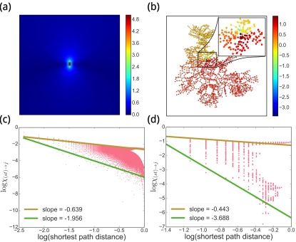
Analogously to the case of vertex perturbation, the effects of edge perturbations can also be solved in the continuum limit, the result being the same as the potential due to an electrical dipole:

$$\xi(\boldsymbol{x}) \propto\frac{\boldsymbol{q}\cdot\boldsymbol{x}}{|\boldsymbol{x}-\boldsymbol{x}_{0}|^{2}},$$ (73)

where $\boldsymbol{q}$ is the unit vector in the direction along which the perturbed edge lie.

This equation shows that unlike the response to vertex perturbation, the response to edge perturbation in a network will be highly directional. The susceptibilities should decay the fastest in the direction along the edge perturbed, according to the power law $d^{-2}$, consistent with the results presented in Jung and Kettemann (2016), but much slower in the orthogonal direction. In Fig. 3 (a,c), we see this direction dependence in a regular square lattice. The lower envelope of the distance-susceptibility plot decays approximately as $d^{-2}$ as expected.

We repeat the same analysis on the Continental European Transmission Network. We see that the susceptibilities are spread even wider for constant distance, indicating a stronger dependence on the orientation of the edge. We notice that the upper envelope in Fig. 3 (d) decays very slowly: $\approx d^{-0.4}$, i.e. there exists a small but nonzero number of nodes that are heavily affected by the perturbation, despite being very far away from the perturbed edge.

VI.4 Explaining the vulnerability of dead ends

The topology of a supply networks determines its local Pecora and Carroll (1998); Motter et al. (2013) as well as global stability Menck et al. (2013); Rohden et al. (2012); Witthaut and Timme (2012). Recently, Menck et al. have shown that dead ends are particularly prone to instabilities Menck et al. (2014). They have measured the robustness of a power grid model to large perturbations at a single node in terms of the so-called basin stability. To this end, the dynamics is simulated after a random perturbation to the steady state at a single node of the network. The basin stability is then defined as the probability that the network relaxes back to the steady state. Extensive Monte Carlo studies show that nodes adjacent to a dead end or dead tree have a particularly small basin stability.

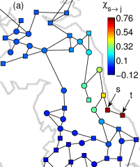
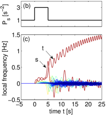
The particular sensitivity of dead ends is directly related to the vertex-to-vertex susceptibility introduced in Sec. IV.4. The main mechanism causing desynchronization at a dead end is shown in Fig. 4. The generation or power injection $P_{s}$ at a vertex $s$ adjacent to a dead end is increased for a short period of time. This perturbation has a strong influence on the vertex $s$ itself but also at the dead end $t$, causing a transient loss of synchrony. For longer times, the vertex $s$ relaxes and resynchronizes with the rest of the network, whereas the dead end $t$ does not. In summary, a perturbation at the vertex $s$ has a large influence on the dynamics of the dead end, while its influence on the bulk of the network is small.

This property if directly mirrored by the vertex-to-vertex susceptibility $\chi_{s\rightarrow j}$. Generally, the susceptibility is largest locally, i.e.  for $j=s$, while it decreases with the distance as discussed above. Only if $s$ is adjacent to a dead end $t$, the non-local susceptibility $\chi_{s\rightarrow t}$ is comparably large. One particular example is shown in Fig. 4 (a). This shows that the non-local impact is strongest at dead ends and thus provides an explanation for their low basin stability.

Figure 4: Large susceptibility and desynchronization at dead ends. (a) The edge susceptibility $\chi_{s\rightarrow j}$ is large for $j=s$ and $j=t$, where $t$ is the dead end adjacent to the vertex $s$. (b,c) Dynamics after a transient increase of the power $P_{s}$ at the vertex $s$. The impact of the perturbation is strongest for the vertices $s$ and $t$. While $s$ relaxes after a short transient period, the dead end $t$ looses synchrony permanently. We consider the topology of the British high-voltage transmission grid as in Fig. 1, of which only a magnified part is shown. We assume that the moments of inertia $M_{j}\equiv M$ and the damping coefficient $D_{j}\equiv D$ are the same for all machines. The machines have power injections of $P_{j}/M=\pm 1\,{\rm s}^{-2}$ and all edges have the transmission capacity $K/M=4\,{\rm s}^{-2}$ and $D/M=0.1\,{\rm s}^{-1}$.

Figure 5: Change of flow magnitudes $|F_{ij}|$ after (a) the damage ($\kappa=-0.1\times K_{st}$) or (b) the complete outage ($\kappa=-K_{st}$) of a single edge (dashed). We compare the prediction of simple linear response approach (26) and the modified formula (80) to the results of a numerical solution of the steady state condition (9). Note the different color scales used in the figure. We consider the topology British high-voltage transmission grid as in Fig. 1, of which only a magnified part is shown.

VII Large perturbations and structural damages

VII.1 From small to large changes

Linear response theory readily predicts how the flow in a network changes after a small perturbation of the network topology. But can it be used to estimate the effects of major changes such as the complete outage of an edge? This is especially important for electric power grids, where transmission line failures repeatedly induce large-scale outages (see, e.g., Albert et al. (2000); Cohen et al. (2001); Motter and Lai (2002); Albert et al. (2004); Buldyrev et al. (2010); Fairley (2004); Pourbeik et al. (2006)). Thus any method that helps to predict the stability of a grid after the failure of a single edge is extremely valuable. For an ad-hoc analysis of network stability in practical applications such methods should be only based on the topological and load properties of the original network and avoid time consuming direct numerical simulations.

We can treat macroscopic changes within a linear response approach if we slightly modify the derivation of edge susceptibilities introduced in Sec. IV.1. As before we keep only terms linear in $\boldsymbol{\xi}$ but we drop the assumption that the perturbations $\kappa_{ij}$ are small. Then Eq. (17) has to be modified as

$$\sum_{i=1}^{N}(K_{ij}+\kappa_{ij})\cos(\phi_{i}-\phi_{j})(\xi_{i}-\xi_{j})$$

$$\qquad=-\sum_{i=1}^{N}\kappa_{ij}\sin(\phi_{i}-\phi_{j}).$$

This set of linear equation is rewritten in matrix form as

$$A_{(st)}\boldsymbol{\xi}=\kappa L_{st}\boldsymbol{q}_{(st)}$$ (75)

with the matrix

$$A_{(st)}=A+\kappa\cos(\phi_{s}-\phi_{t})\,\boldsymbol{q}_{(st)}\boldsymbol{q}_{(st)}^{T},$$ (76)

where the superscript $T$ denotes the transpose of a vector or matrix. The change of the local phases is then obtained by formally solving Eq. (75),

$$\boldsymbol{\xi}=\kappa L_{st}A_{(st)}^{+}\boldsymbol{q}_{(st)}.$$ (77)

In particular we will need the phase differences between two nodes which is given as

$$\xi_{j}-\xi_{i}=\kappa L_{st}\boldsymbol{q}_{(ji)}^{T}A_{(st)}^{+}\boldsymbol{q}_{(st)}.$$ (78)

This expression suggests that we need to calculate the inverse separately for each edge $(s,t)$ if we want to assess the impact of all possible edge failures. However, we can greatly simplify the problem using the Woodbury matrix identity Woodbury , which yields

$$A_{(st)}^{+} =(A+\kappa\cos(\phi_{s}-\phi_{t})\,\boldsymbol{q}_{(st)}\boldsymbol{q}_{(st)}^{T})^{+}$$

$$=A^{+}-A^{+}\boldsymbol{q}_{(st)}(\kappa^{-1}+\boldsymbol{q}_{(st)}^{T}A^{+}\boldsymbol{q}_{(st)})^{+}\boldsymbol{q}_{(st)}^{T}A^{+}$$

We then obtain

$$\boldsymbol{q}_{(ji)}^{T}A_{(st)}^{+}\boldsymbol{q}_{(st)}=\frac{\boldsymbol{q}_{(ji)}^{T}A^{+}\boldsymbol{q}_{(st)}}{1+\kappa\cos(\phi_{s}-\phi_{t})\,\boldsymbol{q}_{(st)}^{T}A^{+}\boldsymbol{q}_{(st)}}\,.$$ (79)

The network flows after the perturbation are now given by

$$F^{\prime\prime}_{ij} =K_{ij}\sin{(\varphi_{j}-\varphi_{i}+\xi_{j}-\xi_{i})}$$

$$=F_{ij}+K_{ij}\cos{(\varphi_{j}-\varphi_{i})}(\xi_{j}-\xi_{i})$$

$$=F_{ij}+\widetilde{K}_{ij}\kappa L_{st}\boldsymbol{q}_{(ji)}^{T}A_{(st)}^{+}\boldsymbol{q}_{(st)}$$

$$=F_{ij}+\,\frac{\kappa L_{st}\widetilde{K}_{ij}(T_{js}-T_{jt}-T_{is}+T_{it})}{1+\kappa\cos(\phi_{s}-\phi_{t})\,(T_{ss}-T_{st}-T_{ts}+T_{tt})}$$

for all edges $(i,j)\neq(s,t)$. This expression differs from Eq. (26) only by the denominator which tends to one in the limit of small perturbations $\kappa\rightarrow 0$. For a macroscopic perturbation the denominator is essential to predict the magnitude of the flow changes correctly. The complete failure of an edge is described by $\kappa=-K_{st}$ such that we obtain

$$F^{\prime\prime}_{ij} =F_{ij}-\,\frac{\widetilde{K}_{ij}(T_{bs}-T_{bt}-T_{as}+T_{at})}{1-\widetilde{K}_{st}(T_{ss}-T_{st}-T_{ts}+T_{tt})}\times F_{st}$$ (80)

for all edges $(i,j)\neq(s,t)$ and $F^{\prime\prime}_{st}=0$ for the failed edge. Similar formulae are used in power engineering, where the fraction is referred to as a Line Outage Distribution Factor (LODF) Wood et al. (2013); Ronellenfitsch et al. (2016b).

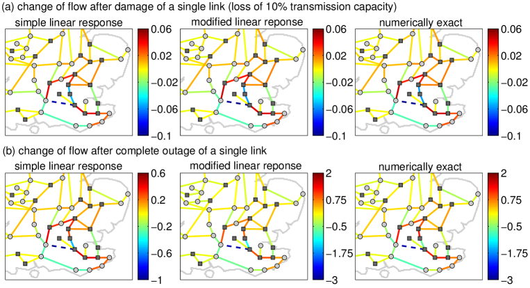
An example of how the damage of a single transmission line affects the flows in a power grid is shown in Fig. 5. We plot the change of the flow magnitude $|F_{ij}|$ predicted by the simple linear response approach (26) and the modified approach (80) in comparison to the actual value obtained from a numerical solution of the steady state condition (9). For a small damage where only $10\%$ of the transmission capacity is lost ($\kappa_{st}=-0.1\times K_{st}$) we find a very good agreement between the predicted and actual values as expected. But even in for a complete breakdown the modified formula (80) provides a very good prediction of the flow changes after the damage. The simpler linear response formula (26) strongly underestimates the flow changes as it neglects the denominator $1-\widetilde{K}_{st}(T_{ss}-T_{st}-T_{ts}+T_{tt})$, which is significantly smaller than one in the current example.

Figure 6: Identification of critical edges using linear response theory. We analyze the effects of the breakdown of a single transmission line for two examples marked by arrows. (a-c) In the upper example, no secondary overloads occur and the grid relaxes back to steady operation after a short transient period. (d-f) In the lower example, linear response theory predicts a secondary overload (black dashed line in d) and consequently the dynamics becomes unstable as shown in panel (f). (a,d) Loads $|F_{ij}^{\prime\prime}/K_{ij}|$ predicted by the modified linear response formula (80) (b,e) Actual load obtained by solving the steady state condition (9). In (e) no steady state exists after the initial breakdown. (c,f) Grid dynamic obtained after the breakdown of the respective edge at $t=0$. We consider the topology of the British high-voltage transmission grid as in Fig. 1, of which only a magnified part is shown. We assume that the moments of inertia $M_{j}\equiv M$ and the damping coefficient $D_{j}\equiv D$ are the same for all machines. The machines have power injections of $P_{j}/M=\pm 1\,{\rm s}^{-2}$ and all edges have the transmission capacity $K/M=4\,{\rm s}^{-2}$ and $D/M=0.1\,{\rm s}^{-1}$.

VII.2 Identification of critical edges

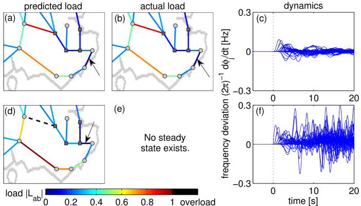
The modified formula (80) can be used to predict impeding overloads and large scale outages in complex supply networks Witthaut et al. (2016). Figure 6 shows the effect of the breakdown of a single transmission line for two examples. In the first example, formula (80) predicts that no overload occurs in agreement with the direct solution of the steady state condition (9). Thus we expect that the grid relaxes to a new steady state after the failure of the respective edge. This prediction is confirmed by a direct numerical simulation of the equations of motion (6). In the second example formula (80) predicts that further overloads occur, i.e. that $|F^{\prime\prime}_{ij}/K_{ij}|>1$ for at least one edge $(i,j)$, after the transmission line $(s,t)$ failed. Indeed, numerical simulations show that no steady state solution of Eq. (9) exists and that the grid becomes unstable and looses synchrony. In the following, we call an edge “critical” if its breakdown induces a desynchronization of the grid. If the grid relaxes back to a steady operation, i.e. an attractively stable synchronized state with $\dot{\phi}_{j}=0$ for all $j$, we call the edge “stable”.

Figure 7: Performance of different classifiers for the prediction of critical edges. (a,b) Histograms of characteristic quantities to identify critical (red) and stable (blue) edges in complex supply networks: (a) load $|L_{st}|$ before breakdown and (b) the maximum load $\max_{(i,j)}|F^{\prime\prime}_{ij}/K_{ij}|$ predicted by linear response theory. (c,d) The performance of the classifiers can be judged by a receiver operating characteristics (ROC) curve, where the sensitivity is plotted vs. the false positive rate for different threshold values $h$. The predicted max. load (solid green line) closely approaches the perfect limit $(0,1)$ and clearly outperforms a classifier based on the load $|L_{st}|$ (dashed). Results are collected for 100 realizations of the British grid with random positions of generators and consumers. One realization is shown in Fig. 5 and Fig. 6.

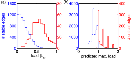
Based on these results we propose to use the maximum load $\max_{(i,j)}|F^{\prime\prime}_{ij}/K_{ij}|$ predicted by the modified linear response formula (80) as a criterion to infer network stability. An edge $(s,t)$ is predicted to be “critical” or “stable” according to the following classification system:

$$\max_{(i,j)}|F^{\prime\prime}_{ij}/K_{ij}|>h\;\Rightarrow\;\mbox{predicted to be critical},$$

$$\max_{(i,j)}|F^{\prime\prime}_{ij}/K_{ij}|\leq h\;\Rightarrow\;\mbox{predicted to be stable},$$ (81)

where $h$ is a threshold value. Bridges, i.e. edges whose removal disconnects the grid are always predicted to be critical.

To test this method, we perform direct numerical simulations of the equations of motion (6) for a large number of test grids, each starting from a stationary state of normal operation and study the influence of the breakdown of a single edge. Examples for both scenarios are shown in Fig. 6. We analyze the coarse-grained structure of the British high-voltage transmission grid Simonsen et al. (2008); Rohden et al. (2012) which has 165 edges. We consider 100 random realizations with random generator positions, thus testing $16\,500$ edges in total. For each out of 100 random realizations, we fix the network topology by randomly selecting half of the nodes to be generators ($P_{j}=+1\,P_{0}$) and the others to be consumers ($P_{j}=-P_{0}$), with $P_{0}=1\,{\rm s}^{-2}$. The transmission capacity of all edges is fixed as $K_{ij}=K_{0}=4\,{\rm s}^{-2}$. One example of such a network is depicted in Fig. 1. Networks not supporting a steady state before any edge breakdown were discarded.

To evaluate the performance of the proposed classification scheme (81) we must first define the possible outcomes of a prediction, where we distinguish between two different kinds of prediction errors:
0 True positive: Edge is predicted critical and is critical.
0 False positive: Edge is predicted critical but is stable.
0 False negative: Edge is predicted stable but is critical.
0 True negative: Edge is predicted stable and is stable.
Generally it is impossible to rule out both false negative and false positive predictions such that a compromise must be achieved. In the current setting, the number of false positive predictions can be minimized by choosing a high value of $h$, while the number of false negative predictions can be minimized by choosing a small value of $h$.

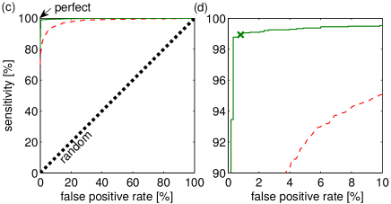
A quantitative assessment of the performance of a classifiers is then provided by a receiver operating characteristics (ROC) curve (Fig. 7) Egan (1975). Here, the true positive rate of the test, also called the sensitivity

$$\mbox{SEN}:=\frac{\#\mbox{true positive predictions}}{\#\mbox{true positive pred.}+\#\mbox{false negative pred.}}$$

is plotted vs. the false positive rate

$$\mbox{FPR}:=\frac{\#\mbox{false positive predictions}}{\#\mbox{false positive pred.}+\#\mbox{true negative pred.}}$$

for different threshold values $h$. For a perfect classifier, the ROC is a point at $(\mbox{FPR},\mbox{SEN})=(0,1)$, while for a fully random classification the ROC curve is a straight line with slope $1$ through the origin. Therefore, a classifier is judged to be the better, the nearer the ROC curve approaches the point $(0,1)$, i.e. the upper left corner of the plot.

Numerical results for 100 realization of the British grid with random generator positions are shown in Fig. 7 (c,d). It is observed that the the classifier (81) closely approaches the perfect limit $(\mbox{FPR},\mbox{SEN})=(0,1)$ and clearly outperforms a classifier based on the load of the edges. Therefore linear response theory provides a very promising approach to identifying critical infrastructures in complex supply networks.

VIII Conclusion and outlook

In summary, we introduced the concepts of vertex susceptibilities and edge susceptibilities as measures of responses to parametric changes in network dynamical systems. They qualitatively distinguish – and quantify – the responses due changes in the properties of units and their interactions, respectively. Focusing on steady state responses of oscillator network characterized by phases or phases and their velocities, we derived explicit forms of such network susceptibilities. We in particular analyzed the role of irregular interaction topologies as those are the least investigated compared to the susceptibilities that are standard in physics. Specifically, we have analyzed how the responses of a network in some given phase locked state depend on the relative location of perturbation and response sites and how the network topologies enter. We linked susceptibilities to established measures, for instance, special cases are known as line outage distribution factors in power grid engineering and susceptibilities are closely related to centrality measures. We explicated an accurate prediction of network responses not only to small perturbation but also after the full breakdown of edges. In power grids, this may be applied, for instance, for an ad-hoc security assessment. Furthermore, network susceptibilities directly reveal weak points of flow networks and may thus be used in the planning and design of future grid extensions and establishing other supply network infrastructures. Finally, the two types of network susceptibilities are generic measures of responses to parameter changes and as such may be straightforwardly generalized across flow, transport and supply networks as well as other network dynamical systems where responses are nonlocal due to genuine collective dynamics.

Appendix A Global edge-to-vertex susceptibility in terms of resistance distance

We start with Eq. (65)

$$T_{ij} =-\frac{1}{2}R_{ij}+\frac{1}{2N}\left(R_{j}^{\rm tot}+R_{i}^{\rm tot}\right)-\frac{\sum_{i,j}R_{ij}}{N^{2}}.$$ (82)

Applying this on Eq. (28), we obtain

$$\frac{\chi^{2}_{(st)}}{L_{st}^{2}} =\sum_{u=1}^{N}(T_{us}-T_{ut})^{2}$$

$$=\sum_{u=1}^{N}\left[-\frac{1}{2}(R_{us}-R_{ut})+\frac{1}{2N}(R_{us}^{\rm tot}-R_{ut}^{\rm tot})\right]^{2}$$

$$=\frac{1}{4N}\left[(R_{s}^{\rm tot}-R_{t}^{\rm tot})\right]^{2}+\frac{1}{4}\sum_{u}(R_{us}-R_{ut})^{2}$$

$$\qquad-\frac{1}{2N}(R_{s}^{\rm tot}-R_{t}^{\rm tot})\sum_{u}(R_{us}-R_{ut})$$

$$=\frac{1}{4N}\left[(R_{s}^{\rm tot}-R_{t}^{\rm tot})\right]^{2}+\frac{1}{4}\sum_{u}(R_{us}-R_{ut})^{2}$$

$$\qquad-\frac{1}{2N}\left[(R_{s}^{\rm tot}-R_{t}^{\rm tot})\right]^{2}$$

$$=-\frac{1}{4N}(R_{s}^{\rm tot}-R_{t}^{\rm tot})^{2}+\frac{1}{4}\sum_{u}(R_{us}-R_{ut})^{2}$$

$$=\frac{N}{4}\left[\frac{1}{N}\sum_{u}(R_{us}-R_{ut})^{2}-\left[\frac{1}{N}\sum_{u}R_{us-R_{ut}}\right]^{2}\right].$$

References

- Strogatz (2001) S. H. Strogatz, Nature 410, 268 (2001).
- Newman (2010) M. E. J. Newman, Networks – An Introduction (Oxford University Press, Oxford, 2010).
- Kuramoto (1975) Y. Kuramoto, in International Symposium on on Mathematical Problems in Theoretical Physics, edited by H. Araki (Springer, New York, 1975), Lecture Notes in Physics Vol. 39, p. 420.
- Kuramoto (1984) Y. Kuramoto, Chemical Oscillations, Waves, and Turbulence (Springer, Berlin, 1984).
- Sompolinsky et al. (1990) H. Sompolinsky, D. Golomb, and D. Kleinfeld, Proc. Natl. Acad. Sci. U.S.A. 87, 7200 (1990).
- Wiesenfeld et al. (1996) K. Wiesenfeld, P. Colet, and S. H. Strogatz, Phys. Rev. Lett. 76, 404 (1996).
- Vladimirov et al. (2003) A. G. Vladimirov, G. Kozireff, and P. Mandel, Europhys. Lett. 61, 613 (2003).
- Heinrich et al. (2011) G. Heinrich, M. Ludwig, J. Qian, B. Kubala, and F. Marquardt, Phys. Rev. Lett. 107, 043603 (2011).
- Rohden et al. (2012) M. Rohden, A. Sorge, M. Timme, and D. Witthaut, Phys. Rev. Lett. 109, 064101 (2012).
- Witthaut and Timme (2012) D. Witthaut and M. Timme, New J. Phys. 14, 083036 (2012).
- Dörfler et al. (2013) F. Dörfler, M. Chertkov, and F. Bullo, Proceedings of the National Academy of Sciences 110, 2005 (2013).
- Motter et al. (2013) A. E. Motter, S. A. Myers, M. Anghel, and T. Nishikawa, Nature Physics 9, 191 (2013).
- Rohden et al. (2014) M. Rohden, A. Sorge, D. Witthaut, and M. Timme, Chaos 24, 013123 (2014).
- Nishikawa and Motter (2015) T. Nishikawa and A. E. Motter, New Journal of Physics 17, 015012 (2015).
- Machowski et al. (2008) J. Machowski, J. Bialek, and J. Bumby, Power system dynamics, stability and control (John Wiley & Sons, New York, 2008).
- Filatrella et al. (2008) G. Filatrella, A. H. Nielsen, and N. F. Pedersen, Eur. Phys. J. B 61, 485 (2008).
- Bergen and Hill (1981) A. R. Bergen and D. J. Hill, IEEE Transactions on Power Apparatus and Systems PAS-100, 25 (1981).
- Wood et al. (2013) A. J. Wood, B. F. Wollenberg, and G. B. Sheblé, Power Generation, Operation and Control (John Wiley & Sons, New York, 2013).
- Ronellenfitsch et al. (2016a) H. Ronellenfitsch, M. Timme, and D. Witthaut, IEEE Transactions on Power Systems PP (2016a).
- D.Manik, D. Witthaut, B. Schaf̈er, M. Matthiae, A. Sorge, M. Rohden, E. Katifori and M. Timme (2014) D.Manik, D. Witthaut, B. Schaf̈er, M. Matthiae, A. Sorge, M. Rohden, E. Katifori and M. Timme, Eur. Phys. J. Special Topics 223, 2527 (2014).
- Skardal et al. (2014) P. S. Skardal, D. Taylor, and J. Sun, Phys. Rev. Lett. 113, 144101 (2014).
- Fiedler (1973) M. Fiedler, Czechoslovak Mathematical Journal 23, 298 (1973).
- Fortunato (2010) S. Fortunato, Physics Reports 486, 75 (2010).
- Simonsen et al. (2008) I. Simonsen, L. Buzna, K. Peters, S. Bornholdt, and D. Helbing, Phys. Rev. Lett. 100, 218701 (2008).
- Ballentine (1998) L. E. Ballentine, Quantum Mechanics – A Modern Development (World Scientific, Singapore, 1998).
- Newman (2005) M. E. J. Newman, Social Networks 27, 39 (2005).
- Brandes and Fleischer (2005) U. Brandes and D. Fleischer, Centrality Measures Based on Current Flow (Springer Berlin Heidelberg, Berlin, Heidelberg, 2005), pp. 533–544.
- Palacios (2001) J. L. Palacios, International Journal of Quantum Chemistry 81, 135 (2001).
- Hutcheon and Bialek (2013) N. Hutcheon and J. W. Bialek, 2013 IEEE Grenoble Conference PowerTech, POWERTECH 2013 pp. 1–5 (2013).
- Jung and Kettemann (2016) D. Jung and S. Kettemann, Phys. Rev. E 94, 012307 (2016).
- Pecora and Carroll (1998) L. M. Pecora and T. L. Carroll, Phys. Rev. Lett. 80, 2109 (1998).
- Menck et al. (2013) P. J. Menck, J. Heitzig, N. Marwan, and J. Kurths, Nature Physics 9, 89 (2013).
- Menck et al. (2014) P. J. Menck, J. Heitzig, J. Kurths, and H. J. Schellnhuber, Nature Comm. 5, 3969 (2014).
- Albert et al. (2000) R. Albert, H. Jeong, and A. Barabási, Nature 406, 378 (2000).
- Cohen et al. (2001) R. Cohen, K. Erez, D. ben Avraham, and S. Havlin, Phys. Rev. Lett. 86, 3682 (2001).
- Motter and Lai (2002) A. E. Motter and Y.-C. Lai, Phys. Rev. E 66, 065102 (2002).
- Albert et al. (2004) R. Albert, I. Albert, and G. L. Nakarado, Phys. Rev. E 69, 025103 (2004).
- Buldyrev et al. (2010) S. V. Buldyrev, R. Parshani, G. Paul, H. E. Stanley, and S. Havlin, Nature 464, 1025 (2010).
- Fairley (2004) P. Fairley, IEEE Spectrum 41, 22 (2004).
- Pourbeik et al. (2006) P. Pourbeik, P. Kundur, and C. Taylor, IEEE Power and Energy Magazine 4, 22 (2006).
- (41) M. A. Woodbury, Inverting modified matrices, Memorandum report 42, Statistical Research Group, Princeton University.
- Ronellenfitsch et al. (2016b) H. Ronellenfitsch, D. Manik, J. Hörsch, T. Brown, and D. Witthaut, arXiv preprint arXiv:1606.07276 (2016b).
- Witthaut et al. (2016) D. Witthaut, M. Rohden, X. Zhang, S. Hallerberg, and M. Timme, Phys. Rev. Lett. 116, 138701 (2016).
- Egan (1975) J. P. Egan, Signal Detection Theory and ROC Analysis (Academic Press, 1975).