Generalized flexibility-rigidity index

Abstract

Flexibility-rigidity index (FRI) has been developed as a robust, accurate and efficient method for macromolecular thermal fluctuation analysis and B-factor prediction. The performance of FRI depends on its formulations of rigidity index and flexibility index. In this work, we introduce alternative rigidity and flexibility formulations. The structure of the classic Gaussian surface is utilized to construct a new type of rigidity index, which leads to a new class of rigidity densities with the classic Gaussian surface as a special case. Additionally, we introduce a new type of flexibility index based on the domain indicator property of normalized rigidity density. These generalized FRI (gFRI) methods have been extensively validated by the B-factor predictions of 364 proteins. Significantly outperforming the classic Gaussian network model (GNM), gFRI is a new generation of methodologies for accurate, robust and efficient analysis of protein flexibility and fluctuation. Finally, gFRI based molecular surface generation and flexibility visualization are demonstrated.

In living organisms, proteins carry out a vast variety of basic functions, such as structure support, catalyzing chemical reactions, and allosteric regulation, through synergistic interactions or correlations. Protein functions and interactions are determined by protein structure and flexibility [10]. The importance of protein structure needs no introduction, while the importance of protein flexibility is often overlooked. Protein flexibility is an intrinsic property of proteins and can be measured by experimental means, including X-ray crystallography, nuclear magnetic resonance (NMR) and single-molecule force spectroscopy, e.g., magnetic tweezer, optical trapping and atomic force microscopy [9]. Flexibility analysis offers a unique channel for theoretical modeling to meet with experimental observations. A variety of theoretical methods, such as normal mode analysis (NMA) [11, 25, 6, 17, 19], graph theory [15], rotation translation blocks (RTB) method [23, 8], and elastic network model (ENM) [4, 3, 2, 14, 24, 18], including Gaussian network model (GNM) [4, 3] and anisotropic network model (ANM) [2], have been proposed. Among them, GNM is often favored due to its accuracy and efficiency [34]. These time-independent methods have been widely used not only for protein fluctuation analysis, but also for entropy estimation. However, they typically suffer from two major drawbacks: 1) ${\cal O}(N^{3})$ scaling in computational complexity with $N$ being the number of elements in the involved matrix and 2) insufficient accuracy in protein B-factor predictions. The above scaling in computational complexity is due to the matrix diagonalization and makes large biomolecules inaccessible to aforementioned methods. Recently, Park et al. have shown that for three sets of structures of small-sized, medium-sized and large-sized, the mean correlation coefficients (MCCs) for NMA and GNM B-factor predictions are respectively below 0.5 and 0.6 [22]. These researchers found that both NMA and GNM fail to work for many structures and deliver negative correlation coefficients [22]. These problems call for the development of accurate, efficient and reliable approaches for the flexibility analysis and entropy calculation of macromolecules.

One strategy to tackle the above-mentioned challenges is to develop matrix-diagonalization-free methods for flexibility analysis. To this end, we have introduced molecular nonlinear dynamics [32], stochastic dynamics [31] and flexibility-rigidity index (FRI) [29, 20]. Our approaches make use of protein network connectivity and centrality to describe protein flexibility and rigidity. In our FRI method, we assume that protein interactions, including those with its environment, fully determine its structure in the given environment. In contrast, protein flexibility and rigidity are fully determined by the structure of the protein and its environment. Therefore, to analyze protein flexibility and rigidity, it is unnecessary to resort to the protein interaction Hamiltonian whenever an accurate protein structure is already available. As a result, FRI bypasses the ${\cal O}(N^{3})$ matrix diagonalization. Our earlier FRI [29] has the computational complexity of ${\cal O}(N^{2})$ and our fast FRI (fFRI) [20] based on a cell lists algorithm [1] is of ${\cal O}(N)$. Anisotropic FRI (aFRI) [20] and multiscale FRI (mFRI) [21] have also been proposed. FRI correlation kernels are utilized to develop generalized GNM (gGNM) and generalized ANM (gANM) methods as well as multiscale GNM (mGNM) and multiscale ANM (mANM) methods [30], which significantly improves their accuracy. In the past two years, we have extensively validated FRI, fFRI, aFRI and mFRI by a set of 364 proteins for accuracy, reliability and efficiency. Our mFRI is about 20% more accurate than GNM on the 364 protein test set [21]. Our fFRI is orders of magnitude faster than GNM on a set of 44 proteins, including one of the largest proteins in the Protein Data Bank (PDB), namely, an HIV virus capsid (1E6J) having 313,236 residues. Our fFRI completes the B-factor prediction of the HIV capsid within 30 seconds on a single-core processor, which would take GNM more than 120 years to accomplish had the computer memory not been a problem [20].

Although various forms of FRI correlation kernels have been introduced, the general mathematical structure of FRI has not been studied. For example, only one rigidity formula and one flexibility formula were proposed[29, 20]. It is interesting to know whether there exists alternative FRI formulations. If so, how do they perform against other existing methods in experimental B-factor predictions? The objective of the present work is to shed lights on these issues. Motivated by the structure of the popular Gaussian surface [13, 12, 16, 26], we propose an alternative rigidity index and a new rigidity density. The latter systematically extends the Gaussian surface to surface densities equipped with a wide variety of FRI correlation kernels. Additionally, we propose normalized rigidity index and normalized rigidity density. The latter behaves like a protein domain indicator [28], which inspires us to introduce a new form of flexibility index and flexibility function. These generalized FRI (gFRI) formulations are extensively validated against experimental data and their performances are systematically compared with a number of other methods. In addition, the new form of flexibility index has been incorporated into aFRI to predict the amplitudes and the directions of atomic fluctuation.

In a molecule with $N$ atoms, we denote $\mathbf{r}_{j}\in\mathbb{R}^{3}$ the position of $j$th atom, and $\|\mathbf{r}_{i}-\mathbf{r}_{j}\|$ the Euclidean distance between $i$th and $j$th atom. An atomic rigidity index is defined as [29, 20]

$$\mu^{1}_{i}=\sum_{\begin{subarray}{c}j=1\end{subarray}}^{N}w_{j}\Phi\left(\|\mathbf{r}_{i}-\mathbf{r}_{j}\|;\eta_{j}\right),$$ (1)

where $w_{j}$ are particle-type related weights that can be set to $w_{j}=1$ for the present work, $\eta_{j}$ are characteristic distances and $\Phi$ is a correlation kernel that satisfies the following admissibility conditions

$$\Phi\left(\|\mathbf{r}_{i}-\mathbf{r}_{i}\|;\eta_{j}\|\right) =1,\quad{\rm as}\quad\|\mathbf{r}_{i}-\mathbf{r}_{j}\|\rightarrow 0,$$ (2)

$$\Phi\left(\|\mathbf{r}_{i}-\mathbf{r}_{j}\|;\eta_{j}\|\right) =0,\quad{\rm as}\quad\|\mathbf{r}_{i}-\mathbf{r}_{j}\|\rightarrow\infty.$$ (3)

Monotonically decaying radial basis functions are all admissible. Commonly used FRI correlation kernels include generalized exponential functions

$$\Phi\left(\|\mathbf{r}_{i}-\mathbf{r}_{j}\|;\eta_{j}\|\right)=e^{-\left(\|\mathbf{r}_{i}-\mathbf{r}_{j}\|/\eta_{j}\right)^{\kappa}},\quad\kappa>0;$$ (4)

and generalized Lorentz functions

$$\Phi\left(\|\mathbf{r}_{i}-\mathbf{r}_{j}\|;\eta_{j}\right)=\frac{1}{1+\left(\|\mathbf{r}_{i}-\mathbf{r}_{j}\|/\eta_{j}\right)^{\nu}},\quad\nu>0.$$ (5)

Many other functions, such as delta sequences of the positive type discussed in an earlier work [27] can be employed as well.

The rigidity index in Eq. (1) was extended into a continuous rigidity density [29, 20]

$$\mu^{1}(\mathbf{r})=\sum_{\begin{subarray}{c}j=1\end{subarray}}^{N}w_{j}\Phi\left(\|\mathbf{r}-\mathbf{r}_{j}\|;\eta_{j}\right).$$ (6)

It has been shown that rigidity density (6) serves as an excellent representation of molecular surfaces [33]. This connection motivates us to generalize the Gaussian surface [13, 12, 16, 26] to a new class of surface densities equipped with a wide variety of FRI correlation kernels ($\Phi\left(\|\mathbf{r}-\mathbf{r}_{j}\|;\eta_{j}\right)$)

$$\mu^{2}(\mathbf{r})=1-\prod_{\begin{subarray}{c}j=1\\ {\bf r}\neq{\bf r}_{j}\end{subarray}}^{n}\left[1-w_{j}\Phi\left(\|\mathbf{r}-\mathbf{r}_{j}\|;\eta_{j}\right)\right].$$ (7)

Since both rigidity densities $\mu^{\alpha}(\mathbf{r}),~{}\alpha=1,2$ represent molecular density at position $\mathbf{r}$, it is convenient to normalize these densities by their maximal values

$$\bar{\mu}^{\alpha}(\mathbf{r})=\frac{\mu^{\alpha}(\mathbf{r})}{\max\limits_{\mathbf{r}\in\mathbb{R}^{3}}\mu^{\alpha}(\mathbf{r})},\quad\alpha=1,2.$$ (8)

In this form, the behaviors of two types of rigidity based molecular surfaces can be easily compared. Additionally, normalized rigidity densities in Eq. (8) can be used as solute domain indicators in implicit solvent models [28]. Obviously, $\max\mu^{\alpha}(\mathbf{r})$ occurs at an atomic position. Therefore, we can define normalized atomic rigidity indexes

$$\bar{\mu}^{\alpha}_{i}=\bar{\mu}^{\alpha}(\mathbf{r}_{i}),\quad\alpha=1,2.$$ (9)

With atomic rigidity indexes, $\bar{\mu}^{\alpha}_{i}$, we denote the flexibility indexes proposed in our earlier work [29, 20] as atomic flexibility indexes of type I [29, 20]

$$f^{\alpha 1}_{i}=\frac{1}{\bar{\mu}^{\alpha}_{i}},\quad\forall i=1,2,\dots,N;\quad\alpha=1,2.$$ (10)

The definition of atomic flexibility indexes is not unique. One of the present objectives is to explore other forms of atomic flexibility indexes. Since the normalized atomic rigidity density can be interpreted as a solute domain indicator, then $1-\bar{\mu}^{\alpha}(\mathbf{r})$ can be regarded as a solvent domain indicator [28, 7]. This motivates us to propose a new form of atomic flexibility indexes

$$f^{\alpha 2}_{i}=1-\bar{\mu}^{\alpha}_{i},\quad\forall i=1,2,\dots,N;\quad\alpha=1,2.$$ (11)

We denote $f^{\alpha 2}_{i}$ as atomic flexibility indexes of type II.

[b] Method Exponential kernels MCC Lorentz kernels MCC gFRI¹¹ $\kappa=1.0,\eta=3.0$ Å 0.625 $\nu=3.0,\eta=3.0$ Å 0.628 gFRI¹² $\kappa=1.0,\eta=4.0$ Å 0.607 $\nu=2.5,\eta=1.0$ Å 0.613 gFRI²¹ $\kappa=1.0,\eta=3.0$ Å 0.604 $\nu=2.5,\eta=1.0$ Å 0.626 gFRI²² $\kappa=1.0,\eta=3.0$ Å 0.621 $\nu=2.5,\eta=2.0$ Å 0.627 FRI^$a$ $\kappa=1.0,\eta=3.0$ Å 0.623 $\nu=3.0,\eta=3.0$ Å 0.626 gGNM^$b$ $\kappa=1.0,\eta=3.0$ Å 0.608 $\nu=3.0,\eta=0.5\text{~{}\AA}$ 0.622 gANM^$c$ $\kappa=2.0,\eta=11.0\text{~{}\AA}$ 0.518 Not available GNM^$d$ Not applicable 0.565

Table 1: Mean correlation coefficients (MCCs) for protein B-factor predictions.

• Results averaged over 365 proteins from Ref. [20].

• Results averaged over 362 proteins from Ref. [30].

• Results averaged over 300 proteins from Ref. [30].

• Results obtained with cutoff distance 7Å  averaged over 365 proteins from Ref. [20].

(a) gFRI¹¹

(b) gFRI¹²

(c) gFRI²¹

(d) gFRI²²

Figure 1: Parameter testing of gFRI methods for exponential (left chart) and Lorentz (right chart) functions. Mean correlation coefficients (MCCs) of B-factor predictions of 364 proteins are plot against choice of $\eta$ for a range of values for $\kappa$ or $\nu$. Note that results with MCCs less 0.45 are not shown.

(a) gFRI¹¹

(b) gFRI¹²

(c) gFRI²¹

(d) gFRI²²

Figure 2: Experimental B-factors (gray) vs predicted B-factors (red) of 1DF4 using the exponential (left) and Lorentz (right) correlation kernels. The optimal parameters for each type of B-factor prediction are described in Table 1.

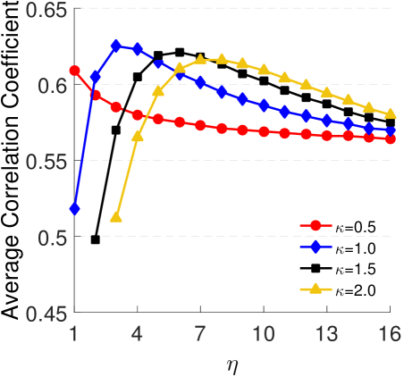
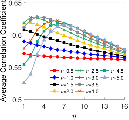
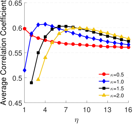
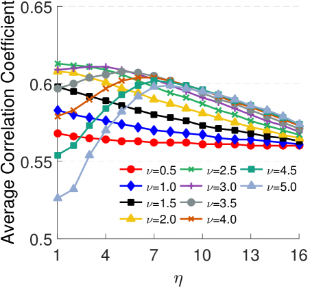
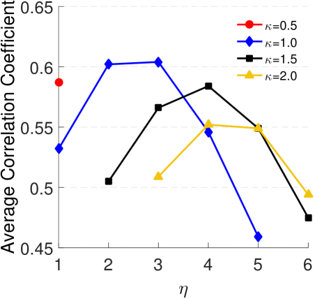
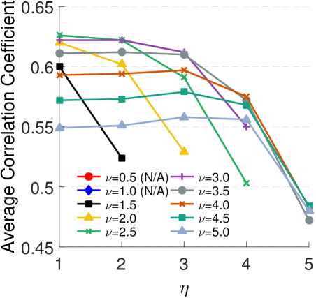
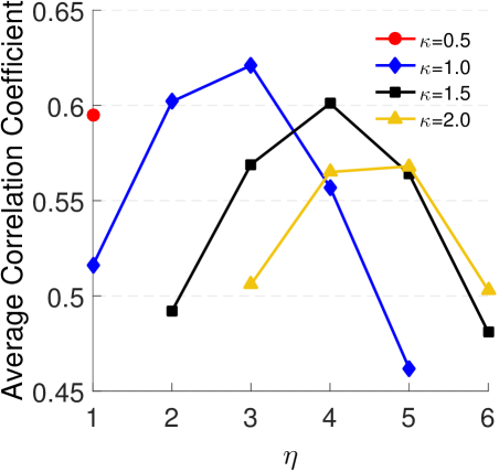
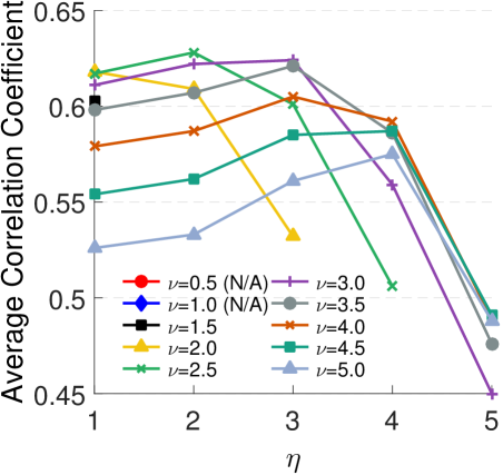
In the rest of this paper, we focus on the exploration of gFRI models associated $f^{\alpha\beta}_{i}$, i.e., $f^{11}_{i}$, $f^{12}_{i}$, $f^{21}_{i}$ and $f^{22}_{i}$, and denote these models as gFRI^αβ. We also study the performance of gFRI for various kernel implementations, namely, generalized exponential and generalized Lorentz correlation kernels.

Due to the proportionality between the atomic flexibility index and the temperature factor at each atom, the theoretical B-factor at $i$th atom, $B_{i}^{\alpha\beta}$, can be expressed as a linear form

$$B_{i}^{\alpha\beta}=a_{\alpha\beta}f^{\alpha\beta}_{i}+b_{\alpha\beta},\quad\forall i=1,2,\dots,N;\alpha=1,2;\beta=1,2$$ (12)

where constants $a_{\alpha\beta}$ and $b_{\alpha\beta}$ are independent of index $i$ and can be estimated by the following minimization process

$$\min_{a_{\alpha\beta},b_{\alpha\beta}}\left\{\sum_{i=1}^{N}\left|B_{i}^{\alpha\beta}-B_{i}^{e}\right|^{2}\right\},$$ (13)

where $B_{i}^{e}$ is the experimental B-factor for the $i$th atom. To quantitatively assess the performance of the proposed gFRI models for the B-factor prediction, we consider correlation coefficient (CC)

$${\rm CC}=\frac{\sum_{i=1}^{N}\left(B_{i}^{e}-\hat{B}_{i}^{e}\right)\left(B_{i}^{\alpha\beta}-\hat{B}_{i}^{\alpha\beta}\right)}{\left[\sum_{i=1}^{N}\left(B_{i}^{e}-\hat{B}_{i}^{e}\right)^{2}\sum_{i=1}^{N}\left(B_{i}^{\alpha\beta}-\hat{B}_{i}^{\alpha\beta}\right)^{2}\right]^{1/2}},$$ (14)

where $\hat{B}^{\alpha\beta}$ and $\hat{B}^{e}$ are, respectively, the statistical averages of theoretical and experimental B-factors.

We consider a set of 364 proteins used in our earlier work [30] and coarse-grained C_α atoms in each protein. Therefore, we set $w_{j}=1$ and use a uniform characteristic distance $\eta_{j}=\eta$ in all of our computations.

We firstly analyze the best parameter set for the B-factor prediction of each rigidity and flexibility type over a range of parameters. Table 1 reveals the optimal parameters and the best MCCs for gFRI^αβ, with $\alpha=1,2$ and $\beta=1,2$. For the sake of visualization, Fig. 1 plots behavior of parameters for exponential and Lorentz kernels in B-factor predictions. It can be seen from Fig. 1 that gFRI²¹ and gFRI²² models are more sensitive to parameter $\eta$ than their gFRI^1β counterparts. Despite having a fewer choices of fitting parameters, gFRI²¹ and gFRI²² models are still able to deliver B-factor predictions as accuracy as those of gFRI^1β models.

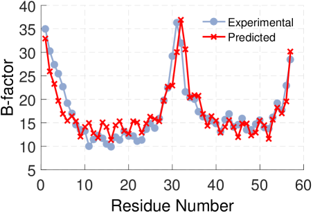
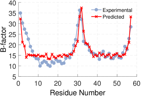
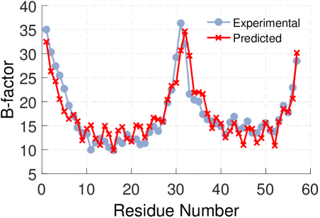
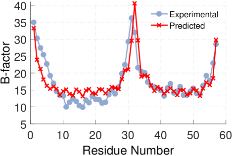
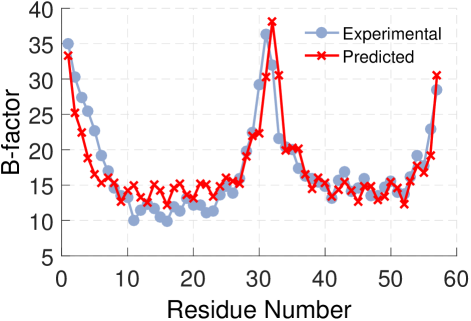
To further demonstrate the accuracy of each type of B-factor predictions for different correlations kernels, we plot predicted B-factors against the experimental ones for protein 1DF4 in Fig. 2. In general, all B-factor prediction approaches produce a similar accuracy, especially when a Lorentz kernel is employed. Moreover, the utilization of exponential type of functions for gFRI¹² and gFRI²¹ B-factor prediction types likely performs a little bit worse than the rest.

For an extended comparison, Table 1 also lists B-factor prediction performances of our earlier FRI [20] method, generalized GNM (gGNM) [30], generalized ANM (gANM) [30] and the classic GNM [4, 3] approaches. The earlier FRI algorithm is the same as gFRI¹¹ in the present work while omits the normalization process (8). By employing the same correlation kernel parameters as of gFRI¹¹, the earlier FRI method gives B-factor predictions similar to those of gFRI¹¹. Specifically, MCCs produced by the previous FRI algorithm for exponential kernel and Lorentz kernel, are, respectively, 0.623 and 0.626. It is noted that the earlier FRI predicted B-factors over 365 proteins [20] while current methods employ the same data set with one left out, 1AGN, due to the unrealistic experimental B-factors.

The gGNM method [30] is an FRI kernel generalization of GNM [4, 3]. In this approach , the $i$th B-factor of a biomolecule can be defined as [4, 3]

$$B_{i}^{\text{gGNM}}=a_{\text{gGNM}}\left(\Gamma^{-1}\right)_{ii},\quad\forall i=1,2,\dots,N,$$ (15)

where $a_{\text{gGNM}}$ is a fitting parameter and $\left(\Gamma^{-1}\right)_{ii}$ is the $i$th diagonal element of the matrix inverse of the generalized Kirchhoff matrix [30]

$$\Gamma_{ij}(\Phi)=\left\{\begin{array}[]{lr}-\Phi\left(\|\mathbf{r}_{i}-\mathbf{r}_{j}\|;\eta_{j}\right),&i\neq j,\vspace*{0.1in}\\ -\sum_{j,j\neq i}^{N}\Gamma_{ij}(\Phi),&i=j.\end{array}\right.$$ (18)

Similarly, the gANM method [30] is an FRI kernel generalization of the classic ANM method [2]. In this approach, the generalized local $3\times 3$ Hessian matrix $H_{ij}$ is written as

$$H_{ij}=-\frac{\Phi\left(\|\mathbf{r}_{i}-\mathbf{r}_{j}\|;\eta_{ij}\right)}{\|\mathbf{r}_{i}-\mathbf{r}_{j}\|^{2}}\left[\begin{array}[]{ccc}(x_{j}-x_{i})(x_{j}-x_{i})&(x_{j}-x_{i})(y_{j}-y_{i})&(x_{j}-x_{i})(z_{j}-z_{i})\\ (y_{j}-y_{i})(x_{j}-x_{i})&(y_{j}-y_{i})(y_{j}-y_{i})&(y_{j}-y_{i})(z_{j}-z_{i})\\ (z_{j}-z_{i})(x_{j}-x_{i})&(z_{j}-z_{i})(y_{j}-y_{i})&(z_{j}-z_{i})(z_{j}-z_{i})\end{array}\right],\forall i\neq j.$$ (22)

We define the diagonal parts as $H_{ii}=-\sum_{i\neq j}H_{ij},\forall i=1,2,\dots,N$. Therefore, the B-factor of $i$th $C_{\alpha}$ in a biomolecule is expressed as

$$B_{i}^{\text{gANM}}=a_{\text{gANM}}\left(H^{-1}\right)_{ii},\quad\forall i=1,2,\dots,N,$$ (23)

where $a_{\text{gANM}}$ is a fitting parameter and $(H^{-1})_{ii}$ is the $i$th diagonal element of the matrix inversion of a matrix formed by generalized local Hessian matrices.

As shown in Table 1, the gGNM prediction with exponential kernel offers the MCC of 0.608 [30] which is as good as gFRI¹² and gFRI²¹ methods and is a bit worse than gFRI¹¹ and gFRI²² approaches. We still find a similar behavior when employing gGNM method with Lorentz kernels. In particular, its MCC is 0.622. On the other hand, the gANM scheme has the worst performance among the considering prediction types. With an MCC found to be 0.518, the gANM approach with exponential kernel is much far behind on the accuracy. Since the gANM prediction with Lorentz type of functions is nowhere close to the acceptable level in term of the accuracy, the result for that case was not reported [30]. Finally, with a cutoff distance of 7Å, the prediction of classic GNM method delivers an MCC of 0.565, which is better than that obtained by gANM, but not as good as any other methods in comparison. Since, GNM is one of the most popular and the most accurate methods for B-factor predictions [34], the current comparison shown in Table 1 indicates that FRI and gFRI are a new generation of more accurate and robust methods for protein B-factor prediction.

Figure 3: Molecular surface of 1DF4 colored by flexibility function with exponential kernel. Left: gFRI¹¹ with $\kappa=1.0$ and $\eta=3.0\text{~{}\AA}$. Right: gFRI¹² with $\kappa=1.0$ and $\eta=4.0\text{~{}\AA}$

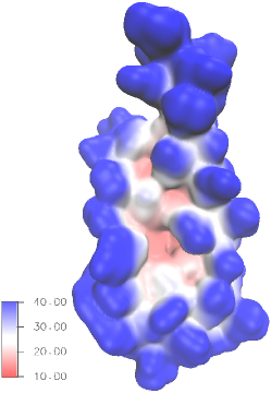
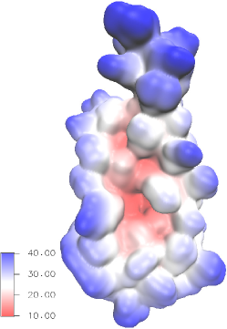
To further compare the B-factor performances between different methods, we introduce two types of continuous flexibility functions.

$$F^{\alpha 1}(\mathbf{r})=\frac{a_{\alpha 1}}{\bar{\mu}^{\alpha}(\mathbf{r})}+b_{\alpha 1},$$ (24)

or

$$F^{\alpha 2}(\mathbf{r})=a_{\alpha 2}\left(1-\bar{\mu}^{\alpha}(\mathbf{r})\right)+b_{\alpha 2},$$ (25)

where $a_{\alpha\beta}$ and $b_{\alpha\beta}$ are determined by minimization (13). These flexibility functions are volumetric and can be projected onto a molecular surface for flexibility visualization. As mentioned earlier, rigidity densities provide excellent molecular surface representations and one can employ either rigidity density $\bar{\mu}^{1}(\mathbf{r})$ or $\bar{\mu}^{2}(\mathbf{r})$ for surface generation. However, for the purpose of surface visualization, rigidity density $\bar{\mu}^{2}(\mathbf{r})$ is not suitable. The reason is that the rigidity formula (7) in the continuous form has to avoid all the grid points near each atomic center. Otherwise rigidity densities would be mostly 1 and the corresponding flexibility functions would be mostly a constant on the molecular surface. This hindrance can be remedied by using interpolation approach as discussed in our previous work [29]. In the present work, we only consider $\bar{\mu}^{1}(\mathbf{r})$ for surface representation and employ $F^{11}(\mathbf{r})$ and $F^{12}(\mathbf{r})$ for flexibility visualization. The parameters for $F^{11}(\mathbf{r})$ and $F^{12}(\mathbf{r})$ follow those of gFRI¹¹ and gFRI¹² as shown in Eqs. (24) and (25), respectively.

Figure 3 depicts the projection of flexibility functions $F^{1\beta}(\mathbf{r})$ onto the isosurface of rigidity density $\bar{\mu}^{1}(\mathbf{r})=0.05$ of protein 1DF4. Parameters $\kappa=1$, $w_{j}=1$ and $\eta_{j}=0.5\text{~{}\AA}$ for all $j=1,\dots,N$ are used in $\bar{\mu}^{1}(\mathbf{r})$ for surface generation. Even though both gFRI¹¹ and gFRI¹² deliver similar B-factor predictions, with MCCs being 0.888 for gFRI¹¹ and is 0.889 for gFRI¹², their flexibility functions ($F^{1\beta}(\mathbf{r})$) behave differently. It can be seen from Fig. 3 that outer region of $F^{11}(\mathbf{r})$ projection contains higher values than its counterpart $F^{12}(\mathbf{r})$, while the inner region of both $F^{1\beta}(\mathbf{r})$ stays almost the same for both methods. This behavior is likely due to the fact that $F^{11}(\mathbf{r})$ is constructed by Eq. (24), which dramatically amplifies small rigidity densities far away from the center of mass of a molecule. In contrast, $F^{12}(\mathbf{r})$ is bound and well defined everywhere.

To predict the amplitudes and directions of atomic fluctuation, ANM [2] is commonly used. Another tool for such purpose is the anisotropic FRI (aFRI) proposed in our previous work [20]. It is interesting to know whether the present flexibility formulation (11) leads to a new algorithm for protein anisotropic motion analysis. To this end, we present a brief review of aFRI theory, which establishes notions for new formulation. In ANM, the Hessian matrix is a global matrix containing $3N\times 3N$ elements with $N$ being a number of atoms. In our aFRI model, depending on one’s interest, the size of the Hessian matrix can vary from $3\times 3$ for a completely local aFRI to $3N\times 3N$ for a completely global aFRI. To construct such a Hessian matrix, we partition all $N$ atoms in a molecule into a total of $M$ clusters $\{c_{1},c_{2},\dots,c_{M}\}$. Each cluster $c_{k}$ with $k=1,\dots,M$ has $N_{k}$ atoms so that $N=\sum_{k=1}^{M}N_{k}$. For convenience, we denote

$$\Phi^{ij}_{uv}=\frac{\partial}{\partial u_{i}}\frac{\partial}{\partial v_{j}}\Phi(\|{\bf r}_{i}-{\bf r}_{j}\|;\eta_{j}),\quad u,v=x,y,z;i,j=1,2,\cdots,N.$$ (26)

Note that for each given $ij$, we define $\Phi^{ij}=\left(\Phi^{ij}_{uv}\right)$ as a local anisotropic matrix

$$\Phi^{ij}=\left(\begin{array}[]{ccc}\Phi^{ij}_{xx}&\Phi^{ij}_{xy}&\Phi^{ij}_{xz}\\ \Phi^{ij}_{yx}&\Phi^{ij}_{yy}&\Phi^{ij}_{yz}\\ \Phi^{ij}_{zx}&\Phi^{ij}_{zy}&\Phi^{ij}_{zz}\end{array}\right).$$ (27)

In the anisotropic flexibility approach, a flexibility Hessian matrix ${\bf F}^{1}(c_{k})$ for cluster $c_{k}$ is defined by

$${\bf F}^{1}_{ij}(c_{k})= -\frac{1}{w_{j}}(\Phi^{ij})^{-1}, \quad i,j\in c_{k};i\neq j;u,v=x,y,z$$ (28)

$${\bf F}^{1}_{ii}(c_{k})= \sum_{j=1}^{N}\frac{1}{w_{j}}(\Phi^{ij})^{-1}, \quad i\in c_{k};u,v=x,y,z$$ (29)

$${\bf F}^{1}_{ij}(c_{k})= 0, \quad i,j\notin c_{k};u,v=x,y,z,$$ (30)

where $(\Phi^{ij})^{-1}$ denotes the unscaled inverse of matrix $\Phi^{ij}$ such that $\Phi^{ij}(\Phi^{ij})^{-1}=|\Phi^{ij}|$.

Motivated by the new form of atomic flexibility indexes (11), we propose another presentation for the flexibility Hessian matrix ${\bf F}^{2}(c_{k})$ as follows

$${\bf F}^{2}_{ij}(c_{k})= -\frac{1}{w_{j}}|\Phi^{ij}|(J_{3}-\Phi^{ij}), \quad i,j\in c_{k};i\neq j;u,v=x,y,z$$ (31)

$${\bf F}^{2}_{ii}(c_{k})= \sum_{j=1}^{N}\frac{1}{w_{j}}|\Phi^{ij}|(J_{3}-\Phi^{ij}), \quad i\in c_{k};u,v=x,y,z$$ (32)

$${\bf F}^{2}_{ij}(c_{k})= 0, \quad i,j\notin c_{k};u,v=x,y,z,$$ (33)

where $J_{3}$ is a $3\times 3$ matrix with every element being one.

We can achieve $3N_{k}$ eigenvectors for $N_{k}$ atoms in cluster $c_{k}$ by diagonalizing ${\bf F}^{\alpha}(c_{k})$, $\alpha=1,2$. Note that, the diagonal part ${\bf F}^{\alpha}_{ii}(c_{k})$, $\alpha=1,2$, has inherent information of all atoms in the system. As a result, we can predict B-factors by employing Eq. (13) for a set of flexibility indexes collected from the diagonal parts

$$f_{i}^{\rm AF_{\alpha}} = {\rm Tr}\left({\bf F}^{\alpha}(c_{k})\right)^{ii},$$ (34)

$$= \left({\bf F}^{\alpha}(c_{k})\right)^{ii}_{xx}+\left({\bf F}^{\alpha}(c_{k})\right)^{ii}_{yy}+\left({\bf F}^{\alpha}(c_{k})\right)^{ii}_{zz},\quad\alpha=1,2.$$ (35)

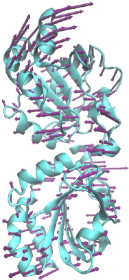
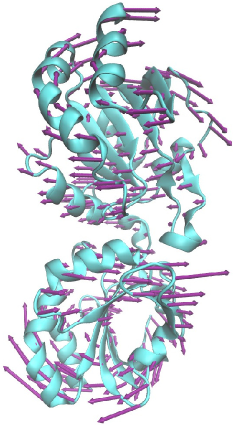
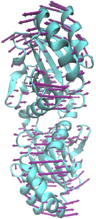
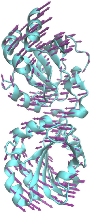
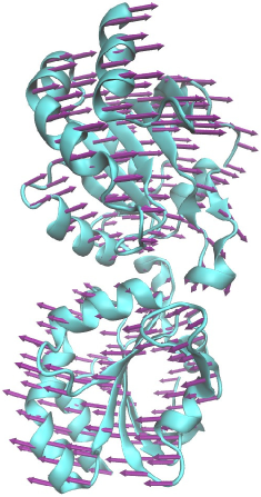
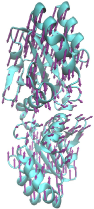
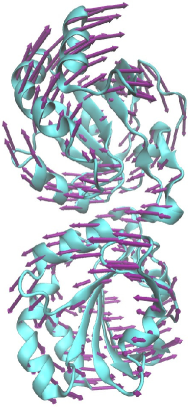
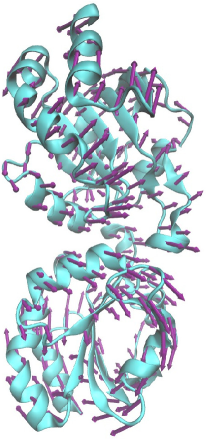
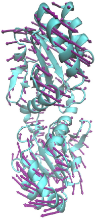
In this work, we compare the protein anisotropic motion predictions by using completely global aFRI models based on the anisotropic flexibility associated with $f_{i}^{\rm AF_{\alpha}}$ and denote these models as $\rm aFRI^{\alpha}$, $\alpha=1,2$. Note that, model $\rm aFRI^{1}$ is already discussed in our previous work [20]and used for a comparison. Figure 4 depict the first three nontrivial isotropic modes of aFRI¹, aFRI² and ANM for protein PBID: 2XHF. The Lorentz kernel is used for both aFRI algorithms with $w_{j}=1,\nu=2,$ and $\eta_{j}=30\text{~{}\AA},\forall j=1,\dots,N$ for aFRI¹, and $w_{j}=1,\nu=2,$and $\eta_{j}=25\text{~{}\AA},\forall j=1,\dots,N$ for aFRI². To obtain ANM prediction, we use Prody v1.8[5] with default settings. It is interesting to see that each algorithm has its own set of collective protein motions. Since there is no exact answer to these fluctuation modes, we cannot conclude which motion prediction is right or wrong.

(a) aFRI¹

(b) aFRI²

(c) ANM

Figure 4: Comparison of modes for protein PDB ID: 2XHF. The top row is generated by using the completely global aFRI¹ with $\nu=2$ and $\eta=30\text{~{}\AA~{}}$. The middle row is generated by using the completely global aFRI² with $\nu=2$ and $\eta=25\text{~{}\AA~{}}$. The bottom row is generated by using ANM with Prody v1.8[5] using default settings.

It needs to point out that the proposed gFRI can be readily incorporated into our fFRI and mFRI methodologies. Additionally, infinitely many possible atomic flexibility indexes of a general functional form $f(\bar{\mu}^{\alpha}_{i})$ can be designed. For example, one can choose $f(\bar{\mu}^{\alpha}_{i})=\Phi\left(\bar{\mu}^{\alpha}_{i};\eta_{0}\right)$ with $\eta_{0}$ being a constant. However, it is not obvious how to design another distinct rigidity density formula. A systematic analysis of these aspects is beyond the scope of the present work.

References

- [1] M. P. Allen and D. J. Tildesley. Computer Simulation of Liquids. Oxford: Clarendon Press, 1987.
- [2] A. R. Atilgan, S. R. Durrell, R. L. Jernigan, M. C. Demirel, O. Keskin, and I. Bahar. Anisotropy of fluctuation dynamics of proteins with an elastic network model. Biophys. J., 80:505 – 515, 2001.
- [3] I. Bahar, A. R. Atilgan, M. C. Demirel, and B. Erman. Vibrational dynamics of proteins: Significance of slow and fast modes in relation to function and stability. Phys. Rev. Lett, 80:2733 – 2736, 1998.
- [4] I. Bahar, A. R. Atilgan, and B. Erman. Direct evaluation of thermal fluctuations in proteins using a single-parameter harmonic potential. Folding and Design, 2:173 – 181, 1997.
- [5] A Bakan, L. M. Meireles, and I. Bahar. Prody: Protein dynamics inferred from theory and experiments. Bioinformatics, 27:1575 –1577, 2011.
- [6] B. R. Brooks, R. E. Bruccoleri, B. D. Olafson, D.J. States, S. Swaminathan, and M. Karplus. Charmm: A program for macromolecular energy, minimization, and dynamics calculations. J. Comput. Chem., 4:187–217, 1983.
- [7] Z. Chen, N. A. Baker, and G. W. Wei. Differential geometry based solvation models I: Eulerian formulation. J. Comput. Phys., 229:8231–8258, 2010.
- [8] Omar N. A. Demerdash and Julie C. Mitchell. Density-cluster NMA: A new protein decomposition technique for coarse-grained normal mode analysis. Proteins:Structure Function and Bioinformatics, 80(7):1766–1779, JUL 2012.
- [9] O. K. Dudko, G. Hummer, and A. Szabo. Intrinsic rates and activation free energies from single-molecule pulling experiments. Phys. Rev. Lett., 96:108101, 2006.
- [10] H. Frauenfelder, S. G. Slihar, and P. G. Wolynes. The energy landsapes and motion of proteins . Science, 254(5038):1598–1603, DEC 13 1991.
- [11] N. Go, T. Noguti, and T. Nishikawa. Dynamics of a small globular protein in terms of low-frequency vibrational modes. Proc. Natl. Acad. Sci., 80:3696 – 3700, 1983.
- [12] J. A. Grant, B. T. Pickup, M. T. Sykes, C. A. Kitchen, and A. Nicholls. The Gaussian Generalized Born model: application to small molecules. Physical Chemistry Chemical Physics, 9:4913–22, 2007.
- [13] J. Andrew Grant, Barry T. Pickup, and Anthony Nicholls. A smooth permittivity function for Poisson-Boltzmann solvation methods. Journal of Computational Chemistry, 22(6):608–640, 2001.
- [14] K. Hinsen. Analysis of domain motions by approximate normal mode calculations. Proteins, 33:417 – 429, 1998.
- [15] D. J. Jacobs, A. J. Rader, L. A. Kuhn, and M. F. Thorpe. Protein flexibility predictions using graph theory. Proteins-Structure, Function, and Genetics, 44(2):150–165, AUG 1 2001.
- [16] Z. Zhang L. Li, C. Li and Emil Alexov. On the dielectric "constant” of proteins: Smooth dielectric function for macromolecular modeling and its implementation in DelPhi. J. Chem. Theory Comput., 9:2126–2136, 2013.
- [17] M. Levitt, C. Sander, and P. S. Stern. Protein normal-mode dynamics: Trypsin inhibitor, crambin, ribonuclease and lysozyme. J. Mol. Biol., 181(3):423 – 447, 1985.
- [18] G. H. Li and Q. Cui. A coarse-grained normal mode approach for macromolecules: an efficient implementation and application to Ca(2+)-ATPase. Bipohys. J., 83:2457 – 2474, 2002.
- [19] J. P. Ma. Usefulness and limitations of normal mode analysis in modeling dynamics of biomolecular complexes. Structure, 13:373 – 180, 2005.
- [20] K. Opron, K. L. Xia, and G. W. Wei. Fast and anisotropic flexibility-rigidity index for protein flexibility and fluctuation analysis. Journal of Chemical Physics, 140:234105, 2014.
- [21] Kristopher Opron, K. L. Xia, and G. W. Wei. Communication: Capturing protein multiscale thermal fluctuations. Journal of Chemical Physics, 142(211101), 2015.
- [22] J. K. Park, Robert Jernigan, and Zhijun Wu. Coarse grained normal mode analysis vs. refined gaussian network model for protein residue-level structural fluctuations. Bulletin of Mathematical Biology, 75:124 –160, 2013.
- [23] F. Tama, F. X. Gadea, O. Marques, and Y. H. Sanejouand. Building-block approach for determining low-frequency normal modes of macromolecules. Proteins: Structure, Function, and Bioinformatics, 41(1):1–7, 2000.
- [24] F. Tama and Y. H. Sanejouand. Conformational change of proteins arising from normal mode calculations. Protein Eng., 14:1 – 6, 2001.
- [25] M. Tasumi, H. Takenchi, S. Ataka, A. M. Dwidedi, and S. Krimm. Normal vibrations of proteins: Glucagon. Biopolymers, 21:711 – 714, 1982.
- [26] Lin Wang, Lin Li, and Emil Alexov. pKa predictions for proteins, RNAs and DNAs with the Gaussian dielectric function using DelPhiPKa. Proteins, 83:2186–2197, 2015.
- [27] G. W. Wei. Wavelets generated by using discrete singular convolution kernels. Journal of Physics A: Mathematical and General, 33:8577 – 8596, 2000.
- [28] G. W. Wei. Differential geometry based multiscale models. Bulletin of Mathematical Biology, 72:1562 – 1622, 2010.
- [29] K. L. Xia, K. Opron, and G. W. Wei. Multiscale multiphysics and multidomain models — Flexibility and rigidity. Journal of Chemical Physics, 139:194109, 2013.
- [30] K. L. Xia, K. Opron, and G. W. Wei. Multiscale gaussian network model (mgnm) and multiscale anisotropic network model (manm). Journal of Chemical Physics, 2015.
- [31] K. L. Xia and G. W. Wei. A stochastic model for protein flexibility analysis. Physical Review E, 88:062709, 2013.
- [32] K. L. Xia and G. W. Wei. Molecular nonlinear dynamics and protein thermal uncertainty quantification. Chaos, 24:013103, 2014.
- [33] K. L. Xia, Z. X. Zhao, and G. W. Wei. Multiresolution persistent homology for excessively large biomolecular datasets. Journal of Chemical Physics, 143:134103, 2015.
- [34] L. W. Yang and C. P. Chng. Coarse-grained models reveal functional dynamics–I. elastic network models–theories, comparisons and perspectives. Bioinformatics and Biology Insights, 2:25 – 45, 2008.