Gaia Data Release 1

Abstract

Context. Gaia Data Release 1 (Gaia DR1) contains astrometric results for more than 1 billion stars brighter than magnitude 20.7 based on observations collected by the Gaia satellite during the first 14 months of its operational phase.

Aims. We give a brief overview of the astrometric content of the data release and of the model assumptions, data processing, and validation of the results.

Methods. For stars in common with the Hipparcos and Tycho-2 catalogues, complete astrometric single-star solutions are obtained by incorporating positional information from the earlier catalogues. For other stars only their positions are obtained, essentially by neglecting their proper motions and parallaxes. The results are validated by an analysis of the residuals, through special validation runs, and by comparison with external data.

Results. For about two million of the brighter stars (down to magnitude $\sim$11.5) we obtain positions, parallaxes, and proper motions to Hipparcos-type precision or better. For these stars, systematic errors depending for example on position and colour are at a level of $\pm 0.3$ milliarcsecond (mas). For the remaining stars we obtain positions at epoch J2015.0 accurate to $\sim$10 mas. Positions and proper motions are given in a reference frame that is aligned with the International Celestial Reference Frame (ICRF) to better than 0.1 mas at epoch J2015.0, and non-rotating with respect to ICRF to within 0.03 mas yr^-1. The Hipparcos reference frame is found to rotate with respect to the Gaia DR1 frame at a rate of 0.24 mas yr^-1.

Conclusions. Based on less than a quarter of the nominal mission length and on very provisional and incomplete calibrations, the quality and completeness of the astrometric data in Gaia DR1 are far from what is expected for the final mission products. The present results nevertheless represent a huge improvement in the available fundamental stellar data and practical definition of the optical reference frame.

1 Introduction

This paper describes the first release of astrometric data from the European Space Agency mission Gaia (Gaia collaboration, Prusti, et al. 2016). The first data release (Gaia collaboration, Brown, et al. 2016) contains provisional results based on observations collected during the first 14 months since the start of nominal operations in July 2014. The initial treatment of the raw Gaia data (Fabricius et al. 2016) provides the main input to the astrometric data processing outlined below.

The astrometric core solution, also known as the astrometric global iterative solution (AGIS), was specifically developed to cope with the high accuracy requirements, large data volumes, and huge systems of equations that result from Gaia’s global measurement principle. A detailed pre-launch description was given in Lindegren et al. (2012), hereafter referred to as the AGIS paper. The present solution is largely based on the models and algorithms described in that paper, with further details on the software implementation in O’Mullane et al. (2011). Nevertheless, comparison with real data and a continuing evolution of concepts have resulted in many changes. One purpose of this paper is to provide an updated overview of the astrometric processing as applied to Gaia Data Release 1 (Gaia DR1). A specific feature of Gaia DR1 is the incorporation of earlier positional information through the Tycho-Gaia astrometric solution (TGAS; Michalik et al. 2015a).

It is important to emphasise the provisional nature of the astrometric results in this first release. Severe limitations are set by the short time period on which the solution is based, and the circumstance that the processing of the raw data – including the image centroiding and cross-matching of observations to sources – had not yet benefited from improved astrometry. Some of the known problems are discussed in Sect. 7. These shortcomings will successively be eliminated in future releases, as more observations are incorporated in the solution, and as the raw data are re-processed using improved astrometric parameters, attitude, and modelling of the instrument geometry.

2 Astrometric content of the data release

The content of Gaia DR1 as a whole is described in Gaia collaboration, Brown, et al. (2016). The astrometric content consists of two parts:

1. The primary data set contains positions, parallaxes, and mean proper motions for 2 057 050 of the brightest stars. This data set was derived by combining the Gaia observations with earlier positions from the Hipparcos (ESA 1997, van Leeuwen 2007a) and Tycho-2 (Høg et al. 2000b) catalogues, and mainly includes stars brighter than visual magnitude 11.5. The typical uncertainty is about 0.3 milliarcsec (mas) for the positions and parallaxes, and about 1 mas yr^-1 for the proper motions. For the subset of 93 635 stars where Hipparcos positions at epoch J1991.25 were incorporated in the solution, the proper motions are considerably more precise, about 0.06 mas yr^-1 (see Table 1 for more statistics). The positions and proper motions are given in the International Celestial Reference System (ICRS; Arias et al. 1995), which is non-rotating with respect to distant quasars. The parallaxes are absolute in the sense that the measurement principle does not rely on the assumed parallaxes of background sources. Moreover, they are independent of previous determinations such as the Hipparcos parallaxes. The primary data set was derived using the primary solution outlined in Sect. 4.1, which is closely related to both TGAS and the Hundred Thousand Proper Motions (HTPM) project (Mignard 2009, unpublished; Michalik et al. 2014).

2. The secondary data set contains approximate positions in the ICRS (epoch J2015.0) for an additional 1 140 622 719 stars and extragalactic sources, mainly brighter than magnitude 20.7 in Gaia’s unfiltered ($G$) band. This data set was derived using the secondary solution outlined in Sect. 4.4, which essentially neglects the effects of the parallax and proper motion during the 14 months of Gaia observations. The positional accuracy is therefore limited by these effects, which typically amount to a few mas but could be much larger for some stars (see Table 2 for statistics).

Gaia DR1 therefore contains a total of 1 142 679 769 sources. Neither data set is complete to any particular magnitude limit. The primary data set lacks the bright stars ($G\lesssim 6$) not nominally observed by Gaia, plus a number of stars with high proper motion (Sect. 5.1). The magnitude limit for the secondary data set is very fuzzy and varies with celestial position. A substantial fraction of insufficiently observed sources is missing in both data sets.

3 Observations and their modelling

Figure 1: Layout of the CCDs in Gaia’s focal plane. Star images move from left to right in the diagram. As the images enter the field of view, they are detected by the sky mapper (SM) CCDs and astrometrically observed by the 62 CCDs in the astrometric field (AF). Basic-angle variations are interferometrically measured using the basic angle monitor (BAM) CCD in row 1 (bottom row in figure). The BAM CCD in row 2 is available for redundancy. Other CCDs are used for the red and blue photometers (BP, RP), radial velocity spectrometer (RVS), and wavefront sensors (WFS). The orientation of the field angles $\eta$ (along-scan, AL) and $\zeta$ (across-scan, AC) is shown at bottom right. The actual origin $(\eta,\zeta)=(0,0)$ is indicated by the numbered yellow circles 1 (for the preceding field of view) and 2 (for the following field of view).

3.1 Input data for the astrometric solutions

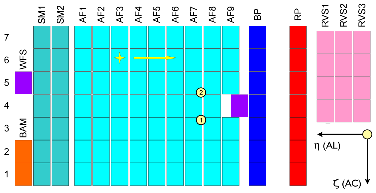
The main input data for the astrometric solutions are the astrometric elementary records, generated by the initial data treatment (Fabricius et al. 2016). Each record holds the along-scan (AL) and across-scan (AC) coordinates for the transit of a source over the sky mapper and astrometric CCDs (Fig. 1), along with the measured fluxes and ancillary information such as the source identifier obtained by cross-matching the observation with the current source list. The record normally contains ten AL coordinate estimates, i.e. one from the sky mapper and nine from the astrometric CCDs; the number of AC measurements ranges from one to ten depending on the window class assigned to the source by the onboard detection algorithm. Most observations in the primary data set are of window class 0 and contain ten AC measurements per record, while the mostly faint sources in the secondary data set have much fewer AC observations. The sky mapper observations were not used in the astrometric solutions for Gaia DR1.

The fundamental AL astrometric observation is the precise time at which the centroid of an image passes the fiducial observation line of a CCD (see Sect. 3.6). This observation time initially refers to the timescale defined by the onboard clock, i.e. the onboard mission timeline (OBMT), but later transformed to the barycentric coordinate time (TCB) of the event by means of the time ephemeris (Sect. 3.4). The OBMT provides a convenient and unambiguous way of labelling onboard events, and will be used below to display, for example, the temporal evolution of calibration parameters. It is then expressed as the number of nominal revolutions of exactly 21600 s OBMT from an arbitrary origin. For the practical interpretation of the plots the following approximate relation between the OBMT (in revolutions) and TCB at Gaia (in Julian years) can be used:

$$\text{TCB}\simeq\text{J}2015.0+(\text{OBMT}-1717.6256\leavevmode\nobreak\ \text{rev})/(1461\leavevmode\nobreak\ \text{rev})\,.$$ (1)

The time interval covered by the observations used for Gaia DR1 starts at OBMT 1078.3795 rev = J2014.5624599 TCB (approximately 2014 July 25, 10:30:00 UTC), and ends at OBMT 2751.3518 rev = J2015.7075471 TCB (approximately 2015 September 16, 16:20:00 UTC), thus spanning 418 days albeit with a number of gaps (see Sect. 3.5).

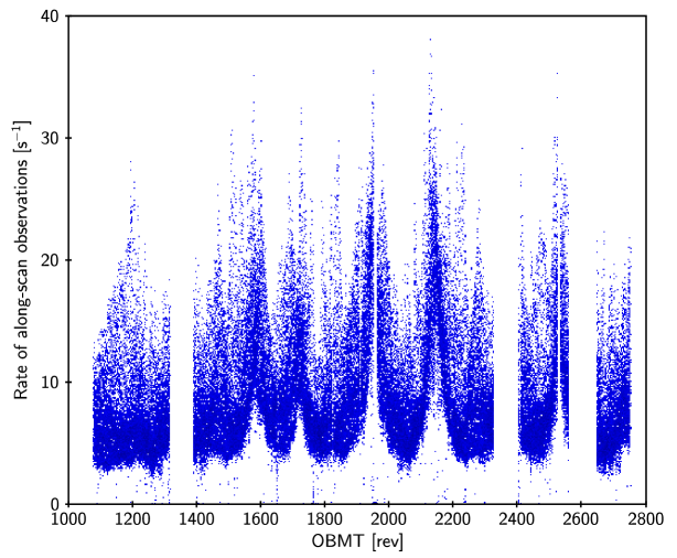
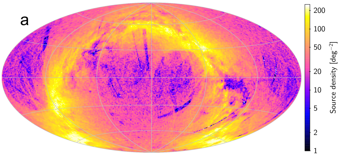
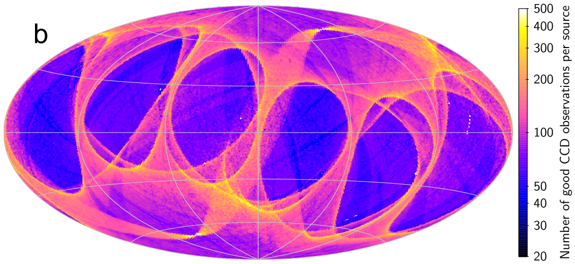
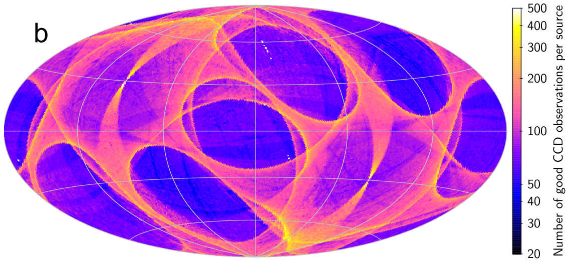
In the primary solution we processed nearly 35 million elementary records, containing some 265 million AL astrometric observations, and a similar number of AC observations, for 2.48 million sources. Figure 2 shows how the rate of these observations varied with time. Peak rates occurred when the scans were roughly along the Galactic plane. On average about 107 AL observations (or 12 field-of-view transits) were processed per source. The actual number of observations per source varies owing to the scanning law and data gaps (see Fig. 5b). For the secondary solution, a total of $1.7\times 10^{10}$ astrometric elementary records were processed.

Auxiliary input data used in the solutions include the initial Gaia source list (IGSL; Smart & Nicastro 2014), ephemerides (Sect. 3.4), and positions at epoch J1991.25 taken from the Hipparcos catalogue (van Leeuwen 2007a, as retrieved from CDS) and the Tycho-2 catalogue (Høg et al. 2000b).

Figure 2: Rate of AL CCD observations input to the primary solution (mean rate per 30 s interval). Time is expressed in revolutions of the onboard mission timeline (OBMT; see text). The three major gaps were caused by decontamination and refocusing activities (Sect. 3.5).

3.2 Celestial reference frame

The Gaia data processing is based on a consistent theory of relativistic astronomical reference systems and involves rigorous modelling of observable quantities. Various components of the model are gathered in the Gaia relativity model (GREM; Klioner 2003, 2004). The primary coordinate system used for the astrometric processing of Gaia data is the Barycentric Celestial Reference System (BCRS; Soffel et al. 2003). The BCRS has its origin at the solar-system barycentre and its axes are aligned with the ICRS. The time-like coordinate of the BCRS is TCB. The motions of Gaia and other solar-system objects are thus described by the space-like coordinates of the BCRS, $x(t)$, $y(t)$, $z(t)$, using TCB as the independent time variable $t$. The motions of all objects beyond the solar system are also parametrised in terms of BCRS coordinates (Sect. 3.3), but here the independent time variable $t$ should be understood as the time at which the event would be observed at the solar-system barycentre, i.e. the time of observation corrected for the Rømer delay. This convention is necessitated by the in general poor knowledge of distances beyond the solar system.

The reference frame for the positions and proper motions in Gaia DR1 is in practice defined by the global orientation of positions at the two epochs J1991.25 and J2015.0. From the construction of the Hipparcos and Tycho-2 catalogues, the positions of stars around epoch J1991.25, as given in these catalogues, represent the best available realisation of the optical reference frame at that epoch, with an estimated uncertainty of 0.6 mas in each axis (Vol. 3, Ch. 18.7 in ESA 1997). On the other hand, by using the Gaia observations of quasars with positions in the ICRS accurately known from Very Long Baseline Interferometry (VLBI), it was possible to align the global system of positions in Gaia DR1 to the ICRS with an estimated uncertainty of $<\,$0.1 mas at epoch J2015.0 (Sect. 4.3). From the 23.75 yr time difference between these epochs it follows that the resulting proper motion system should have no global rotation with respect to ICRS at an uncertainty level of about 0.03 mas yr^-1.

The Gaia observations of quasars over several years will eventually permit a non-rotating optical reference frame to be determined entirely from Gaia data, independent of the Hipparcos reference frame, and to a much higher accuracy than in the current release.

3.3 Astrometric modelling of the sources

The basic astrometric model is described in Sect. 3.2 of the AGIS paper and assumes uniform space motion relative to the solar-system barycentre. In a regular AGIS solution this is applicable only to the subset of well-behaved “primary sources”, used to determine the attitude, calibration, and global parameters, while “secondary sources” may require more complex modelling. In Gaia DR1 the basic model is applied to all stellar and extragalactic objects, which are thus treated effectively as single stars. The distinction between primary and secondary sources is instead based on the type of prior information incorporated in the solutions (Sects. 4.1 and 4.4).

In the basic model the apparent motion of a source, as seen by Gaia, is completely specified by six kinematic parameters, i.e. the standard five astrometric parameters $(\alpha,\,\delta,\,\varpi,\,\mu_{\alpha*},\,\mu_{\delta})$, defined below, and the radial velocity $v_{r}$. For practical reasons $v_{r}=0$ is assumed in Gaia DR1 for all objects, meaning that perspective acceleration is not taken into account (see below). All the parameters refer to the reference epoch $t_{\text{ep}}=\text{J2015.0\leavevmode\nobreak\ TCB}$.

The time-dependent coordinate direction from Gaia towards an object beyond the solar system is therefore modelled, in the BCRS, as the unit vector

$$\@vec{\bar{u}}(t)=\Bigl{\langle}\@vec{r}+(t_{\text{B}}-t_{\text{ep}})\left(\@vec{p}\mu_{\alpha*}+\@vec{q}\mu_{\delta}+\@vec{r}\mu_{r}\right)-\@vec{b}_{\text{G}}(t)\varpi/A_{\text{u}}\Bigr{\rangle}\,,$$ (2)

where $t$ is the time of observation (TCB); $\@vec{p}$, $\@vec{q}$, and $\@vec{r}$ are orthogonal unit vectors defined in terms of the astrometric parameters $\alpha$ and $\delta$,

$$\@vec{p}=\begin{bmatrix}-\sin\alpha\\ \cos\alpha\\ 0\end{bmatrix},\quad\@vec{q}=\begin{bmatrix}-\sin\delta\cos\alpha\\ -\sin\delta\sin\alpha\\ \cos\delta\end{bmatrix},\quad\@vec{r}=\begin{bmatrix}\cos\delta\cos\alpha\\ \cos\delta\sin\alpha\\ \sin\delta\end{bmatrix};\quad$$ (3)

$t_{\text{B}}=t+\@vec{r}^{\prime}\@vec{b}_{\text{G}}(t)/c$ is the time of observation corrected for the Rømer delay ($c=$ speed of light); $\@vec{b}_{\text{G}}(t)$ is the barycentric position of Gaia at the time of observation; and $A_{\text{u}}$ is the astronomical unit. $\mu_{\alpha*}=\mu_{\alpha}\cos\delta$ and $\mu_{\delta}$ are the components of proper motion along $\@vec{p}$ (towards increasing $\alpha$) and $\@vec{q}$ (towards increasing $\delta$), respectively, and $\varpi$ is the parallax. $\mu_{r}=v_{r}\varpi/A_{\text{u}}$ is the radial proper motion related to the perspective acceleration discussed below.

The modelling of stellar proper motions neglects all effects that could make the apparent motions of stars non-linear in the $\sim$24 year interval between the Hipparcos/Tycho observations and the Gaia observations. Thus, orbital motion in binaries and perturbations from invisible companions are neglected, as well as the perspective secular changes caused by non-zero radial velocities. The published proper motions should therefore be interpreted as the mean proper motions over this time span, rather than as the instantaneous proper motions at the reference epoch J2015.0. The published positions, on the other hand, give the barycentric directions to the stars at J2015.0.

Perspective acceleration is a purely geometrical effect caused by the changing distance to the source and changing angle between the velocity vector and the line of sight (e.g. van de Kamp 1981). It is fully accounted for in Eq. (2) by means of the term containing $\mu_{r}$. The perspective acceleration (in mas yr^-2) is proportional to the product of the star’s parallax, proper motion, and parallax, and is therefore very small except for some nearby, high-velocity stars (cf. de Bruijne & Eilers 2012). In the current astrometric solutions it is effectively ignored by assuming $v_{r}=0$, and hence $\mu_{r}=0$, for all objects. This is acceptable for Gaia DR1 provided that the resulting proper motions are interpreted as explained above. In future releases perspective acceleration will be taken into account, whenever possible, using radial-velocity data from Gaia’s onboard spectrometer (RVS; Gaia collaboration, Prusti, et al. 2016).

3.4 Relativistic model and auxiliary data

The coordinate direction $\@vec{\bar{u}}$ introduced in Sect. 3.3 should be transformed into the observed direction $\@vec{u}$ (also known as proper direction) as seen by Gaia. This is done using the previously mentioned GREM (Klioner 2003, 2004).

The transformation essentially consists of two steps. First, the light propagation from the source to the location of Gaia is modelled in the BCRS. In this process, the influence of the gravitational field of the solar system is taken into account in full detail. It includes the gravitational light-bending caused by the Sun, the major planets and the Moon. Both post-Newtonian and major post-post-Newtonian effects are included. For observations close to the giant planets the effects of their quadrupole gravitational fields are taken into account in the post-Newtonian approximation. The non-stationarity of the gravitational field, caused by the translational motion of the solar-system bodies, is also properly taken into account. On the other hand, no attempt is made to account for effects of the gravitational field outside the solar system. This plays a role only in cases when its influence is variable on timescales comparable with the duration of observations, e.g. in various gravitational lensing phenomena.

The second step is to compute the observed direction $\@vec{u}$ from the computed BCRS direction of light propagation at the location of Gaia. To this end, a special physically adequate (local) proper reference system for the Gaia spacecraft, known as the centre-of-mass reference system (CoMRS), is used as explained in Klioner (2004). At this step we take into account the stellar aberration caused by the BCRS velocity of Gaia’s centre of mass, as well as certain smaller general-relativistic effects.

The model requires several kinds of auxiliary data. These include the Gaia ephemeris (the BCRS position and velocity of Gaia), the solar-system ephemeris (the positions and velocities of all gravitating bodies of the solar system used in the model), and the time ephemeris used to convert the reading of the Gaia onboard clock into TCB.

The Gaia ephemeris is provided by the European Space Operation Centre (ESOC) based on radiometric observations of the spacecraft and using standard orbit reconstruction procedures (Gaia collaboration, Prusti, et al. 2016). The Gaia orbit determination satisfies the accuracy requirements imposed by Gaia DR1: the uncertainty of the BCRS velocity of Gaia is believed to be considerably below 10 mm s^-1. For future releases, the Gaia orbit will be verified in a number of ways at the level of 1 mm s^-1, which is needed to reach the accuracy goal of the project.

The solar system ephemeris used in the Gaia data processing is the INPOP10e ephemeris (Fienga et al. 2016) parametrised by TCB. The time ephemeris for the Gaia clock is constructed from special time-synchronisation observations of the spacecraft (Gaia collaboration, Prusti, et al. 2016), using a consistent relativistic model for the proper time of the Gaia spacecraft.

The CoMRS also provides a consistent definition of the spacecraft attitude in the relativistic context. The reference system that is aligned with the instrument axes is known as the scanning reference system (SRS; Lindegren et al. 2012). The attitude discussed in Sect. 3.5 represents a pure spatial rotation between CoMRS and SRS.

3.5 Attitude model

The attitude model is fully described in Sect. 3.3 of the AGIS paper. It uses cubic splines to represent the four components of the attitude quaternion as functions of time. The basic knot sequence for the present solutions is regular with a knot interval of 30 s. Knots of multiplicity four are placed at the beginning and end of the knot sequence, allowing the spline to be discontinuous at these points, and similarly around imposed data gaps. Such gaps were introduced around the fourth and fifth mirror decontaminations (Gaia collaboration, Prusti, et al. 2016), spanning OBMT 1316.490–1389.113 and 2324.900–2401.559 rev, respectively, and in connection with the refocusing of the following field of view at OBMT 1443.963–1443.971 rev, and of the preceding field of view at OBMT 2559.0–2650.0 rev (see Fig. 2). Additional gaps were placed around 45 micrometeoroid hits identified in provisional solutions. These gaps are typically less than 10 s, but reach 1–1.5 min in some cases. The total number of knots is 980 666, yielding 3 922 648 attitude parameters.

A longer knot interval of 180 s was used in the first phases of the solution (phase A and B in Fig. 4). At the end of phase B, a spline with 30 s knot interval was fitted to the attitude estimate at that point, and the iterative solution continued with the shorter interval. This procedure speeds up the convergence considerably without degrading the final, converged solution.

As described in Sect. 5.2.4 of the AGIS paper, the attitude updating uses a regularisation parameter $\lambda$ to constrain the updated quaternion to unit length. The adopted value is $\lambda=\sqrt{10^{-7}}$.

3.6 Geometric instrument calibration model

The astrometric instrument consists of the optical telescope with two viewing directions (preceding and following field of view), together with the sky mapper (SM) and astrometric field (AF) CCDs, see Fig. 1. The geometric calibration of the instrument provides an accurate transformation from pixel coordinates on the CCDs to the field angles $(\eta,\,\zeta)$. Depending on the field of view in which an object was observed, the field angles define its observed direction in the SRS at the time of observation, $t$. The observation time is the precise instant when the stellar image crosses a fiducial observation line on the CCD. The AL calibration describes the geometry of the observation line as a function $\eta(\mu)$ of the AC pixel coordinate $\mu$. The latter is a continuous variable covering the 1966 pixel columns, running from $\mu=13.5$ at one edge of the CCD (minimum $\zeta$) to $\mu=1979.5$ at the opposite edge (maximum $\zeta$). $\eta(\mu)$ additionally depends on a number of parameters including the CCD index ($n$), field-of-view index ($f$), CCD gate ($g$), and time. The temporal dependence is described by means of discrete calibration intervals, $t_{j}\leq t<t_{j+1}$. In the current configuration these intervals are not longer than 3 days, but have additional breakpoints inserted at appropriate times, e.g. when a significant jump is seen in the onboard metrology signal (see Sect. 3.7).

The current model also includes a dependence on the window class ($w$) of the observation (see footnote 1). Ideally the location of the image centroid should not depend on the size of the window used to calculate the centroid, i.e. on the window class. (Nor should it depend on, for example, the colour and magnitude of the star.) However, this can only be achieved after the CCD image line-spread function (LSF) and point-spread function (PSF) have been calibrated using astrometric, attitude, and geometric calibration information from a previous AGIS. Since this outer processing loop has not yet been closed, a dependence on the window class is introduced in the geometric calibration model as a temporary measure.

The detailed specification of the calibration model and all its dependencies is made in the framework of the generic calibration model briefly described in Sect. 3.4 of the AGIS paper. The model used for the current astrometric solution is further explained in Appendix A.1.

3.7 Use of onboard metrology (BAM)

Integrated with the Gaia instrument is a laser-interferometric device, the basic angle monitor (BAM; Gaia collaboration, Prusti, et al. 2016), which measures variations of the basic angle on timescales from minutes to days. Line-of-sight variations are monitored by means of two interference patterns, one per field of view, projected on a dedicated CCD next to the sky mappers (Fig. 1). An example of the line-of-sight variations is given in the top part of Fig. 11, which shows fringe positions derived from the interference pattern in the preceding field of view. The basic angle variations are calculated as the differential line-of-sight variation between the two fields of view.

Because the BAM was not designed for long-term stability, it measures reliably only the relative variations on timescales shorter than a few days. The absolute value of the basic angle ($\Gamma$) and its evolution on longer timescales are routinely determined in the astrometric solution as part of the geometric instrument calibration (Sect. 3.6). On the relevant (short) timescales, the variations of the basic angle, reconstructed from the BAM data, exhibit very significant periodic patterns (amplitude $\sim$1 mas; see Gaia collaboration, Prusti, et al. 2016) as well as discontinuities, trends, and other features, all of which may be used to correct the astrometric observations. For Gaia DR1 a somewhat conservative approach has been adopted, in which only the most prominent features of the BAM signal are taken into account in the astrometric solution. These include the major discontinuities and the regular part of the periodic variations. The discontinuities are taken into account by appropriate choice of calibration boundaries as described in Sect. 3.6. The corrections derived from the periodic variations of the BAM signal are discussed in Appendix A.2.

4 Astrometric solutions

Figure 3: Logic of the astrometric solutions contributing to Gaia DR1. The top boxes show the number of sources input to the solutions, and the different priors used to constrain the solutions. The number of sources finally kept in Gaia DR1 is substantially smaller. The TGAS and the auxiliary quasar solutions work in the Hipparcos reference frame; the final primary and secondary solutions are aligned with ICRF. All sources are also treated by the secondary solution; in the end, a decision is made for each source whether to select the primary or secondary solution for Gaia DR1, or none. The results of the auxiliary quasar solution are only used for alignment, calibration, and validation purposes. The quasar results in Gaia DR1 come, with few exceptions, from the secondary solution.

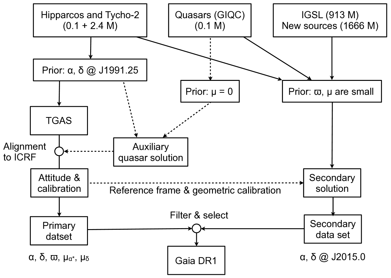
The astrometric results in Gaia DR1 come from several interdependent solutions, as illustrated in Fig. 3 and detailed below.

4.1 Primary solution (TGAS)

The primary solution for Gaia DR1 uses the positions of $\sim$114 000 sources from the re-reduced Hipparcos catalogue (van Leeuwen 2007a), and an additional 2.36 million positions from the Tycho-2 catalogue (Høg et al. 2000b) as prior information for a joint Tycho-Gaia astrometric solution (TGAS; Michalik et al. 2015a). Only the positions at J1991.25 (for the Hipparcos stars) or at the effective Tycho-2 observation epoch (taken to be the mean of the $\alpha$ and $\delta$ epochs) were used, together with the uncertainties and correlations given in the catalogues. It is important that the parallaxes from the Hipparcos catalogue and the proper motions from the Hipparcos and Tycho-2 catalogues were not used. This ensures that the calculated parallaxes and proper motions in the primary solution are independent of the corresponding values in the earlier catalogues, which can therefore usefully be compared with the new results (see Appendices B and C).

Figure 4: Convergence of the iterative astrometric solution for the primary data set. The solid curve is the typical size of parallax updates in each iteration; the dashed curve is the typical size of AL residuals (in $\mu$as). The letters refer to the main phases of the iterative scheme: A – iterations with 180 s attitude knot interval (Sect. 3.5) and simplified calibration model; B – iterations with full calibration model; C – using 30 s attitude knot interval; D – Hipparcos alignment active (see text); E – auxiliary quasar solution (Sect. 4.2) using a fixed attitude; F – source and calibration updates after final alignment of the attitude to the ICRS (Sect. 4.3).

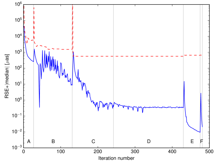
The primary solution cyclically updates the source, attitude, and calibration parameters, using a hybrid scheme alternating between so-called simple iterations and the conjugate gradient algorithm (Bombrun et al. 2012, Lindegren et al. 2012. While the conjugate gradient method in general converges much faster than simple iterations, the latter method allows the minimisation problem to be modified between iterations, which is necessary in the adaptive weighting scheme used to identify outliers and to estimate the excess source noise and excess attitude noise. The iterative solution for the primary data set of Gaia DR1 was done in several phases, using successively more detailed modelling, as summarised in Fig. 4. For example, a simplified calibration model was used during the first phase (A), and a longer attitude knot interval was used in the first two phases (A and B), compared with all subsequent phases.

In phase D the source and attitude parameters were aligned with the Hipparcos reference frame after each iteration. This was done by applying a global rotation to the TGAS positions at epoch J2015.0, such that for the Hipparcos stars they were globally consistent, in a robust least-squares sense, with the positions obtained by propagating the Hipparcos catalogue to that epoch. By construction, the TGAS positions extrapolated back to J1991.25 coincide with the Hipparcos positions used as priors at that epoch. Therefore, at this stage of the processing, both the TGAS positions and the TGAS proper motions were strictly in the Hipparcos reference frame. The subsequent auxiliary quasar solution in phase E (Sect. 4.2) computed the positions and parallaxes of the quasars, as well as the calibration parameters for window class 1 and 2 ($G\gtrsim 13$; see footnote 1) needed in the secondary solution (Sect. 4.4). The attitude, however, was not updated in the auxiliary quasar solution, which was therefore kept in the Hipparcos reference frame during this phase. As explained in Sect. 4.3, the final reference frame of Gaia DR1 was obtained by a further small rotation applied in phase F.

The iteration scheme described above uses both AL and AC observations with their formal uncertainties provided by the initial data processing. However, we found that the resulting parallax values depend in a systematic way on the uncertainties assigned to the AC observations. The origin of this effect is not completely understood, although it is known that the AC measurements are biased, owing to the rudimentary PSF calibration used in the pre-processing of the current data sets. To eliminate the effect in the present solution we artificially increased the AC formal standard uncertainties 1000 times in the last source update in phase E (for the quasars) and in phase F (for the primary data set).

As shown by the dashed curve in Fig. 4, the width of the residual distribution does not decrease significantly after the first $\sim$150 iterations. (The slight increase from phase E is caused by the addition of the faint quasars, which on average have larger residuals than the TGAS sources.) However, the subsequent few hundred iterations in phase C and D, during which the updates (solid curve) continue to decrease, are extremely important for reducing spatially correlated errors. It is difficult to define reliable convergence criteria even for idealised simulations (Bombrun et al. 2012), but the typical updates in parallax should be at least a few orders of magnitude smaller than the aimed-for precision. In the present solution the final updates are typically well below 1 microarcsec ($\mu$as). During phase E there was a further rapid decrease of the updates, down to ${\sim}0.01\leavevmode\nobreak\ \mu$as. However, since the attitude parameters were not updated in phase E, it is probable that truncation errors remain at roughly the same level as at the end of phase D.

Uncertainty estimates

It is known from simulations (e.g. Sect. 7.2 in the AGIS paper) that the formal uncertainties of the astrometric parameters calculated in AGIS underestimate the actual errors. One reason for this is that the covariances are computed from the truncated $5\times 5$ normal matrices of the individual sources, thus ignoring the contributing uncertainties from other unknowns such as attitude and calibration parameters. The relation between formal and actual uncertainties may under certain conditions be derived from a statistical comparison with an independent data set. The Hipparcos parallaxes offer such a possibility, which is explored in Appendix B. For the Gaia DR1 parallaxes of Hipparcos sources the following inflation factor is derived:

$$F\equiv\sigma_{\varpi}/\varsigma_{\varpi}\simeq\sqrt{a^{2}+(b/\varsigma_{\varpi})^{2}}\,.$$ (4)

Here $\varsigma_{\varpi}$ is the formal parallax uncertainty calculated in the source update of AGIS (i.e. from the inverse $5\times 5$ normal matrix of the astrometric parameters), $\sigma_{\varpi}$ is the actual parallax uncertainty estimated from a comparison with the Hipparcos parallaxes, and $a=1.4$, $b=0.2$ mas are constants (see Fig. 14). Although this relation was derived only for a subset of the sources (i.e. Hipparcos entries) and for one specific parameter (parallax), it has been applied, for lack of any better recipe, to all the sources and all astrometric parameters in the primary data set. This was done by applying the factor $F^{2}$, calculated individually for each source, to its $5\times 5$ covariance matrix. This leaves the correlation coefficients among the five astrometric parameters unchanged. All astrometric uncertainties for the primary solution quoted in this paper refer to the inflated values $\sigma_{\alpha*}=F\varsigma_{\alpha*}$, etc., except when explicitly stated otherwise.

4.2 Auxiliary quasar solution

Some 135 000 quasars from the Gaia initial quasar catalogue (GIQC; Andrei et al. 2009, 2012, 2014) were included towards the end of the solution (phase E in Fig. 4). By assuming that these sources have negligible proper motions (the prior was set to $0\pm 0.01$ mas yr^-1 in each component) it was possible to solve the positions and parallaxes for most of them as described by Michalik & Lindegren (2016). At the end of phase E these objects had positions and parallaxes with median (inflated) standard uncertainties of about 1 mas. Their proper motions, although formally solved as well, are not meaningful as they merely reflect the prior information: they are practically zero. Because the attitude was not updated in the auxiliary quasar solution, the quasar positions were obtained in the same reference frame as the preceding TGAS (at the end of phase D).

The resulting positions and parallaxes are used for two purposes: (i) the positions for a subset of sources with accurately known positions from VLBI are used to align the Gaia DR1 reference frame with the extragalactic radio frame as described in Sect. 4.3; and (ii) as described in Appendix C.2 the observed parallaxes for the whole set of ${\sim}10^{5}$ quasars provide a valuable check of the parallax zero point and external accuracy of the solutions.

The quasar solution also provides the geometric instrument calibration for the fainter sources observed using window class 1 and 2 (see footnote 1). This part of the calibration is needed for the secondary solution (Sect. 4.4), but cannot be obtained in the primary solution of the brighter sources, which are normally observed using window class 0.

The positions and parallaxes from the auxiliary quasar solution are not contained in Gaia DR1. The positions for these objects are instead computed in the secondary solution (Sect. 4.4) and become part of the secondary data set along with data for other quasars and most of the Galactic stars. The secondary solution does not constrain the proper motion of the quasars to a very small value, as in the auxiliary quasar solution, and the resulting positions are therefore slightly different. After correction for the different reference frames of Gaia DR1 and the auxiliary quasar solution (Sect. 4.3), the RSE difference between the quasar positions in the two solutions is 1.22 mas in right ascension and 0.94 mas in declination, with median differences below 0.05 mas.

4.3 Alignment to the ICRF

Ideally, the alignment procedure should define a celestial coordinate system for the positions and proper motions in Gaia DR1 that (i) is non-rotating with respect to distant quasars; and (ii) coincides with the ICRF at J2015.0. (Because the ICRF is also non-rotating, the two frames should then coincide at all epochs.) For Gaia DR1 the time interval covered by the observations is too short to constrain the spin of the reference frame by means of the measured proper motions of quasars, as will be done for future releases. Instead, a special procedure was devised, which relies on the assumption that the Hipparcos catalogue, at the time of its construction, was carefully aligned with the ICRF (Kovalevsky et al. 1997). Since the primary solution takes the Hipparcos positions at J1991.25 as priors, it should by construction be properly aligned with the ICRF at that epoch. However, this is not sufficient to constrain the spin of the Gaia DR1 reference frame. For that we must also require that the quasar positions at J2015.0 are consistent with ICRF2. It may seem surprising that the combination of stellar positions at J1991.25 with quasar positions at J2015.0 can be used to constrain the spin, given that the two sets of objects do not overlap. However, this is achieved by the auxiliary quasar solution, in which the observations of both kinds of objects are linked by a single set of attitude and calibration parameters. The practical procedure is somewhat more complicated, as it uses the Hipparcos reference frame as a provisional intermediary for the proper motions.

The current physical realisation of the ICRS at radio wavelengths is ICRF2 (Ma et al. 2009, Fey et al. 2015), which contains precise VLBI positions of 3414 compact radio sources, of which 295 are defining sources. Among the sources in the auxiliary quasar solution (Sect. 4.2) we find 2191 objects with acceptable astrometric quality ($\epsilon_{i}<20$ mas and $\sigma_{\text{pos,max}}<100$ mas; cf. Eq. 12) that, based on positional coincidence (separation $<$ 150 mas), are likely to be the optical counterparts of ICRF2 sources. (The remaining $\sim$1200 ICRF2 sources may have optical counterparts that are too faint for Gaia.) As described in Sect. 4.2, the positions computed in the auxiliary quasar solution are expressed in a provisional reference frame aligned with the Hipparcos reference frame. They are here denoted $(\alpha_{\text{H}},\,\delta_{\text{H}})$ to distinguish them from the corresponding positions $(\alpha,\,\delta)$ in the final Gaia DR1 reference frame. The VLBI positions of the matched ICRF2 sources are denoted $(\alpha_{\text{ICRF}},\,\delta_{\text{ICRF}})$. The position differences for the matched sources are generally less than 10 mas, and exceed 50 mas for less than a percent of the sources.

If the orientation of the optical positions with respect to the ICRF2 is modelled by an infinitesimal solid rotation, we have

$$\left.\begin{aligned} (\alpha_{\text{H}}-\alpha_{\text{ICRF}})\cos\delta&=(\@vec{\varepsilon}\times\@vec{r})^{\prime}\@vec{p}=\phantom{-}\@vec{q}^{\prime}\@vec{\varepsilon}\\ \delta_{\text{H}}-\delta_{\text{ICRF}}&=(\@vec{\varepsilon}\times\@vec{r})^{\prime}\@vec{q}=-\@vec{p}^{\prime}\@vec{\varepsilon}\end{aligned}\quad\right\}\,,\quad$$ (5)

where $\@vec{p}$ and $\@vec{q}$ are given by Eq. (3) and $\@vec{\varepsilon}$ is a vector whose components are the rotation angles around the ICRS axes. Equation (5) involves approximations that break down for sources close to the celestial poles, or if $|\@vec{\varepsilon}|$ is too large. None of these conditions apply in the present case. Rigorous formulae are given in Sect. 6.1 of the AGIS paper.

A robust weighted least-squares estimation of the orientation parameters, based on the 262 defining sources in ICRF2 with separation $<$ 150 mas, gives

$$\@vec{\varepsilon}\equiv\begin{bmatrix}\varepsilon_{X}\\ \varepsilon_{Y}\\ \varepsilon_{Z}\end{bmatrix}=\begin{bmatrix}-2.990\\ +4.387\\ +1.810\end{bmatrix}\leavevmode\nobreak\ \text{mas}\,.$$ (6)

The robust fitting retains 260 of the defining sources. The uncertainty, estimated by bootstrap resampling (Efron & Tibshirani 1994), is about 0.04 mas in each component. For comparison, a solution based instead on the 1929 non-defining sources in ICRF2 gives $\@vec{\varepsilon}=[-2.933,\,+4.453,\,+1.834]^{\prime}$ mas. Using both defining and non-defining sources, but taking only one hemisphere at a time ($\pm X$, $\pm Y$, $\pm Z$), gives solutions that never differ from Eq. (6) by more than 0.15 mas in any component. These tests suggest that the result (6) is robust at the 0.1 mas level. Figure 22 shows the distribution of positional residuals with respect to this solution. The median total positional residual $(\Delta\alpha{*}^{2}+\Delta\delta^{2})^{1/2}$ is 0.61 mas for the 262 matched defining sources, and 1.27 mas for the 1929 non-defining sources. The 90th percentiles are, respectively, 2.7 mas and 7.2 mas. Additional statistics are given in Appendix C.2.

The reference frame of Gaia DR1 is defined by its orientations at the two epochs J1991.25 (set by the Hipparcos reference frame at that epoch) and J2015.0 (set by the Gaia observations of ICRF2 sources). Assuming that the Hipparcos positions were accurately aligned at the earlier epoch, the result in Eq. (6) implies that the Hipparcos reference frame has a rotation relative to ICRF2 of $\@vec{\omega}=(23.75\leavevmode\nobreak\ \text{yr})^{-1}\@vec{\varepsilon}$ or

$$\begin{bmatrix}\omega_{X}\\ \omega_{Y}\\ \omega_{Z}\end{bmatrix}\simeq\begin{bmatrix}-0.126\\ +0.185\\ +0.076\end{bmatrix}\leavevmode\nobreak\ \text{mas\leavevmode\nobreak\ yr${}^{-1}$}\,.$$ (7)

This has an uncertainty of about 0.03 mas yr^-1 in each axis, mainly from the uncertainty of the orientation of the Hipparcos reference frame at J1991.25, estimated to be 0.6 mas in each axis (Vol. 3, Ch. 18.7 in ESA 1997), divided by the epoch difference. To put the Hipparcos proper motions on the Gaia DR1 reference frame therefore requires the correction

$$\left.\begin{aligned} \mu_{\alpha*}&=\mu_{\alpha*\text{H}}-\@vec{q}^{\prime}\@vec{\omega}\\ \mu_{\delta}&=\mu_{\delta\text{H}}\phantom{j}+\@vec{p}^{\prime}\@vec{\omega}\end{aligned}\quad\right\}\,.$$ (8)

It can be noted that the inferred rotation in Eq. (7) is well within the claimed uncertainty of the spin of the Hipparcos reference frame, which is 0.25 mas yr^-1 per axis (Vol. 3, Ch. 18.7 in ESA 1997).

Subsequent iterations of the primary data set (phase F in Fig. 4) and the secondary solution (Sect. 4.4) used a fixed attitude estimate, obtained by aligning the attitude from phase D with the Gaia DR1 reference frame. This was done by applying the time-dependent rotation $\@vec{\varepsilon}+(t-t_{\text{ep}})\@vec{\omega}$, where $t_{\text{ep}}=\text{J2015.0}$. The procedure for rotating the attitude is described in Sect. 6.1.3 of the AGIS paper. With this transformation the axes of the positions in Gaia DR1 and those of the ICRF2 are aligned with an estimated uncertainty of 0.1 mas at epoch J2015.0.

4.4 Secondary solution

At the end of the primary and quasar solutions (Sects. 4.1–4.2) the final attitude estimate is aligned with ICRF2 to within a fraction of a mas, and calibration parameters consistent with this attitude are available for all magnitudes (different gates and window classes). The secondary solution uses this fixed set of attitude and calibration parameters to estimate the positions of sources in the secondary data set. Contrary to the primary solution, this can be done one source at a time, as it does not involve complex iterations between the source, attitude, and calibration parameters.

For Gaia DR1 the sources in the secondary data set are all treated as single stars. The astrometric model is therefore the same as for the primary sources (Sect. 4.1) with five parameters per source. Lacking a good prior position at some earlier epoch, as for the Tycho-2 stars, it is usually not possible to reliably disentangle the five astrometric parameters of a given star based on the observations available for the current release. Therefore, only its position at epoch J2015.0 is estimated. The neglected parallax and proper motion add some uncertainty to the position, which is included in the formal positional uncertainties. The latter are calculated using the recipe in Michalik et al. (2015b), based on a realistic model of the distribution of stellar parallaxes and proper motions as functions of magnitude and Galactic coordinates. The inflation factor in Eq. (4) is not applicable to these uncertainties and was not used for the secondary data set.

5 Results

Table 1: Statistical summary of the 2 million sources in the primary data set of Gaia DR1.

	All primary sources				Hipparcos subset
Quantity	10%	50%	90%		10%	50%	90%	Unit
Standard uncertainty in $\alpha$ ($\sigma_{\alpha*}=\sigma_{\alpha}\cos\delta$)	0.147	0.254	0.601		0.158	0.224	0.391	mas
Standard uncertainty in $\delta$ ($\sigma_{\delta}$)	0.140	0.233	0.530		0.150	0.218	0.378	mas
Standard uncertainty in $\varpi$ ($\sigma_{\varpi}$)	0.242	0.322	0.644		0.229	0.283	0.499	mas
Standard uncertainty in $\mu_{\alpha*}$ ($\sigma_{\mu\alpha*}$)	0.500	1.132	2.671		0.035	0.064	0.129	mas yr-1
Standard uncertainty in $\mu_{\delta}$ ($\sigma_{\mu\delta}$)	0.441	0.867	1.957		0.031	0.056	0.109	mas yr-1
Semi-major axis of error ellipse in position ($\sigma_{\text{pos,\,max}}$)	0.203	0.319	0.753		0.196	0.263	0.475	mas
Semi-major axis of error ellipse in proper motion ($\sigma_{\text{pm,\,max}}$)	0.715	1.322	3.189		0.038	0.069	0.137	mas yr-1
Excess source noise ($\epsilon_{i}$)	0.299	0.478	0.855		0.347	0.572	1.185	mas
Number of field-of-view transits input to the solution ($N$)	8	15	25		7	14	25
Number of good CCD observations AL used in the solution ($n_{\text{good}}$)	57	99	185		51	93	180
Fraction of bad CCD observations AL ($n_{\text{bad}}/(n_{\text{good}}+n_{\text{bad}})$)	0.0	0.0	2.0		0.0	0.0	1.8	%
Normalised difference to Hipparcos proper motion ($\Delta Q$)	–	–	–		0.33	2.35	11.32
Magnitude in Gaia’s unfiltered band ($G$)	9.27	11.04	12.05		6.84	8.28	9.70	mag

Figure 5: Summary statistics for the 2 million sources in the primary data set of Gaia DR1: (a) density of sources; (b) number of good CCD observations per source; (c) excess source noise. The maps use an Aitoff projection in equatorial (ICRS) coordinates, with origin $\alpha=\delta=0$ at the centre and $\alpha$ increasing from right to left. The mean density (a) and median values (b and c) are shown for sources in cells of about 0.84 deg². A small number of empty cells are shown in white.

Figure 6: Summary statistics for the 2 million sources in the primary data set of Gaia DR1: (a) density of sources; (b) number of good CCD observations per source; (c) excess source noise. These maps use an Aitoff projection in Galactic coordinates, with origin $l=b=0$ at the centre and $l$ increasing from right to left. The mean density (a) and median values (b and c) are shown for sources in cells of about 0.84 deg². A small number of empty cells are shown in white.

5.1 Primary data set

For each source the primary solution gives the five astrometric parameters $\alpha$, $\delta$, $\varpi$, $\mu_{\alpha*}$, and $\mu_{\delta}$ together with various statistics indicating the quality of the results. The most important statistics are

• the standard uncertainties of the astrometric parameters: $\sigma_{\alpha*}=\sigma_{\alpha}\cos\delta$, $\sigma_{\delta}$, $\sigma_{\varpi}$, $\sigma_{\mu\alpha*}$, and $\sigma_{\mu\delta}$;

• the ten correlation coefficients among the five parameters: $\rho(\alpha,\delta)$, $\rho(\alpha,\varpi)$, etc.;

• the number of field-of-view transits of the source used in the solution: $N$;

• the number of good and bad CCD observations of the source: $n_{\text{good}}$, $n_{\text{bad}}$;

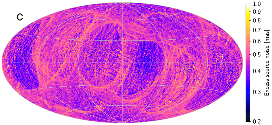
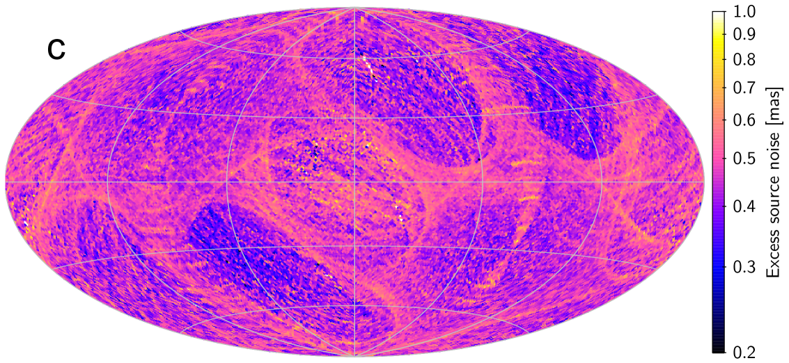
• the excess source noise: $\epsilon_{i}$. This is meant to represent the modelling errors specific to a given source, i.e. deviations from the astrometric model in Eq. (2) caused, for example, by binarity (see Sect. 3.6 in the AGIS paper). Thus, it should ideally be zero for most sources. In the present primary solution nearly all sources obtain significant excess source noise ($\sim$0.5 mas) from the high level of attitude and calibration modelling errors. An unusually large value of $\epsilon_{i}$ (say, above 1–2 mas) could nevertheless indicate that the source is an astrometric binary or otherwise problematic.

Additional statistics can be calculated from the standard uncertainties and correlation coefficients. These include the semi-major axes of the error ellipses in position and proper motion. Let $C_{00}=\sigma_{\alpha*}^{2}$, $C_{11}=\sigma_{\delta}^{2}$, and $C_{01}=\sigma_{\alpha*}\sigma_{\delta}\rho(\alpha,\delta)$ be elements of the $5\times 5$ covariance matrix of the astrometric parameters. The semi-major axis of the error ellipse in position is

$$\sigma_{\text{pos,\,max}}=\sqrt{\frac{1}{2}(C_{00}+C_{11})+\frac{1}{2}\sqrt{(C_{11}-C_{00})^{2}+4C_{01}^{2}}}\,,$$ (9)

with a similar expression for the semi-major axis of the error ellipse in proper motion, $\sigma_{\text{pm,\,max}}$, using the covariance elements $C_{33}$, $C_{44}$, and $C_{34}$.

For the subset in common with the Hipparcos catalogue one additional statistic is computed: $\Delta Q$, which measures the difference between the proper motion derived in the primary (TGAS) solution and the proper motion given in the Hipparcos catalogue. It is computed as

$$\Delta Q=\begin{bmatrix}\Delta\mu_{\alpha*}&\Delta\mu_{\delta}\end{bmatrix}\left(\@vec{C}_{\text{pm,\,T}}+\@vec{C}_{\text{pm,\,H}}\right)^{-1}\begin{bmatrix}\Delta\mu_{\alpha*}\\ \Delta\mu_{\delta}\end{bmatrix}\,,$$ (10)

where $\Delta\mu_{\alpha*}=\mu_{\alpha*\text{T}}-\mu_{\alpha*\text{H}}$ and $\Delta\mu_{\delta}=\mu_{\delta\text{T}}-\mu_{\delta\text{H}}$ are the proper motion differences, with T and H designating the values from respectively TGAS and the Hipparcos catalogue. $\@vec{C}_{\text{pm,\,T}}$ is the $2\times 2$ covariance submatrix of the TGAS proper motions and $\@vec{C}_{\text{pm,\,H}}$ the corresponding matrix from the Hipparcos catalogue. The new reduction of the raw Hipparcos data by van Leeuwen (2007a) was used, as retrieved from CDS, with covariances computed as described in Appendix B of Michalik et al. (2014). For the calculation in Eq. (10) the Hipparcos proper motions were first transformed to the Gaia DR1 reference frame by means of Eq. (8) and then propagated to epoch J2015.0, assuming zero radial velocity. $\Delta Q$ is therefore sensitive to all deviations from a purely linear tangential proper motion, including perspective effects. If the proper motion errors in TGAS and in the Hipparcos catalogue are independent and Gaussian with the given covariances, then $\Delta Q$ is expected to follow a chi-squared distribution with two degrees of freedom, i.e. $\text{Pr}(\Delta Q>x)=\exp(-x/2)$.

Figure 7: Summary statistics for the 2 million sources in the primary data set. The five maps along the main diagonal show, from top-left to bottom-right, the standard uncertainties in $\alpha$, $\delta$, $\varpi$, $\mu_{\alpha*}$, $\mu_{\delta}$. The ten maps above the diagonal show the correlation coefficients, in the range $-1$ to $+1$, between the corresponding parameters on the main diagonal. All maps use an Aitoff projection in equatorial (ICRS) coordinates, with origin $\alpha=\delta=0$ at the centre and $\alpha$ increasing from right to left. Median values are shown in cells of about 0.84 deg².

The primary solution gives astrometric results for about 2.48 million sources. Unreliable solutions are removed by accepting only sources with

$$\sigma_{\varpi}<1\leavevmode\nobreak\ \text{mas}\quad\text{and}\quad\sigma_{\text{pos,\,max}}<20\leavevmode\nobreak\ \text{mas}\,.$$ (11)

Here $\sigma_{\varpi}$ is the standard uncertainty in parallax from Eq. (4), and $\sigma_{\text{pos,\,max}}$ is the semi-major axis of the error ellipse in position at the reference epoch (J2015.0). The second condition removes a small fraction of stars with extremely elongated error ellipses.

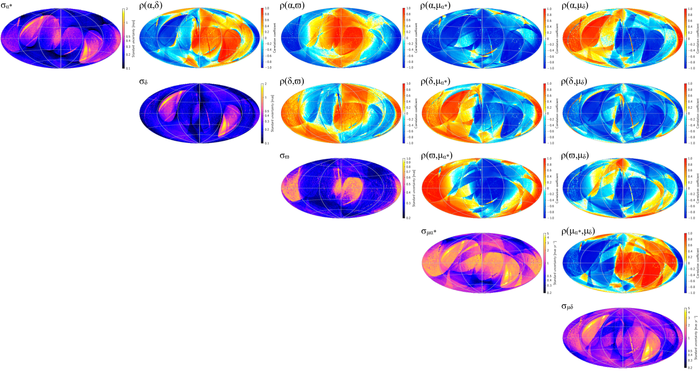
Applying the filter in Eq. (11) results in a set of 2 086 766 sources with accepted primary solutions. However, for a source to be included in Gaia DR1 it must also have valid photometric information. The primary data set therefore gives astrometric parameters for 2 057 050 sources together with their estimated standard uncertainties, correlations among the five parameters, and other quality indicators. A statistical summary is presented in Table 1. Separate statistics are given for the subset of Hipparcos sources, which have rather different uncertainties in proper motion owing to the more accurate positions at the Hipparcos epoch. Figures 5–7 show the variation of some statistics with celestial position. The distribution of $\Delta Q$ for the Hipparcos subset is discussed in Appendix C.1.

In the primary data set, the standard uncertainties of the positions at epoch J2015.0 and of the parallaxes are dominated by attitude and calibration errors in the Gaia observations. They therefore show little or no systematic dependence on magnitude. For the proper motions, on the other hand, the dominating error source is usually the positional errors at J1991.25 resulting from the Hipparcos and Tycho-2 catalogues. The uncertainties in proper motion therefore show a magnitude dependence mimicking that of the positional uncertainties in these catalogues.

To preserve the statistical integrity of the data set, no filtering was applied based on the actual values of the astrometric parameters. Thus, the primary data set contains 30 840 (1.5%) negative parallaxes. The most negative parallax is $-24.82\pm 0.63$ mas, but even this provides valuable information, e.g. that there are parallaxes that are wrong by at least 40 times the stated uncertainty. However, owing to a technical issue in the construction of the initial source list, several nearby stars with high proper motion are missing in the Hipparcos subset of Gaia DR1. In particular, the 19 Hipparcos stars with total proper motion $\mu>3500$ mas yr^-1 are missing, including the five nearest stars HIP 70891 (Proxima Cen), 71681 ($\alpha^{2}$ Cen), 71683 ($\alpha^{1}$ Cen), 87937 (Barnard’s star), and HIP 54035. ($\alpha^{1}$ and $\alpha^{2}$ Cen would in any case have been rejected because they are too bright.)

Table 2: Statistical summary of the 1141 million sources in the secondary data set of Gaia DR1.

Quantity		10%	50%	90%		Unit
Standard uncertainty in $\alpha$ ($\sigma_{\alpha*}=\sigma_{\alpha}\cos\delta$)		0.285	1.802	12.871		mas
Standard uncertainty in $\delta$ ($\sigma_{\delta}$)		0.257	1.568	11.306		mas
Semi-major axis of error ellipse in position ($\sigma_{\text{pos,\,max}}$):
$G<16$ (7% of the secondary data set)		0.106	0.255	4.118		mas
$G=16{-}17$ (7%)		0.182	0.484	11.105		mas
$G=17{-}18$ (13%)		0.284	0.761	11.534		mas
$G=18{-}19$ (22%)		0.501	1.444	13.027		mas
$G=19{-}20$ (31%)		0.986	2.816	16.314		mas
$G=20{-}21$ (20%)		2.093	7.229	21.737		mas
all magnitudes (100%)		0.349	2.345	15.699		mas
Excess source noise ($\epsilon_{i}$)		0.000	0.594	2.375		mas
Number of field-of-view transits input to the solution ($N$)		7	13	26
Number of good CCD observations AL used in the solution ($n_{\text{good}}$)		41	71	157
Fraction of bad CCD observations AL ($n_{\text{bad}}/(n_{\text{good}}+n_{\text{bad}})$)		0.0	0.0	2.0		%
Magnitude in Gaia’s unfiltered band ($G$)		16.49	19.02	20.32		mag

Figure 8: Density of sources in the secondary data set of Gaia DR1: (a) all 1141 million sources in the secondary data set; (b) the 685 million sources in common with the IGSL; (c) the 456 million new sources. These maps use an Aitoff projection in equatorial (ICRS) coordinates, with origin $\alpha=\delta=0$ at the centre and $\alpha$ increasing from right to left. Mean densities are shown for sources in cells of about 0.84 deg².

Figure 9: Density of sources in the secondary data set of Gaia DR1: (a) all 1141 million sources in the secondary data set; (b) the 685 million sources in common with the IGSL; (c) the 456 million new sources. These maps use an Aitoff projection in Galactic coordinates, with origin $l=b=0$ at the centre and $l$ increasing from right to left. Mean densities are shown for sources in cells of about 0.84 deg².

5.2 Secondary data set

The secondary solution gives approximate positions for more than 2.5 billion entries, including more than 1.5 billion “new sources” created in the process of cross-matching the Gaia detections to the source list (see Sect. 4 in Fabricius et al. 2016).

Many of the new sources are spurious, and a suitable criterion had to be found to filter out most of the bad entries. On the other hand, for uniformity of the resulting catalogue, it is desirable that the very same criteria do not reject too many of the solutions using observations cross-matched to the initial source list. By comparing the distributions of various quality indicators for the two kinds of sources, the following criterion was found to provide sensible rejection of obviously spurious sources while retaining nearly all solutions for sources in the initial source list:

$$N\geq 5\quad\text{and}\quad\epsilon_{i}<20\leavevmode\nobreak\ \text{mas}\quad\text{and}\quad\sigma_{\text{pos,max}}<100\leavevmode\nobreak\ \text{mas}\,.$$ (12)

$N$ is the number of field-of-view transits used in the solution, $\epsilon_{i}$ is the excess source noise (Sect. 5.1), and $\sigma_{\text{pos,max}}$ the semi-major axis of the error ellipse in position at the reference epoch. The excess source noise is essentially a measure of the astrometric consistency of the $N$ transits. The first two conditions therefore mean that the source should have been detected at least five times at positions consistent within some 20 mas. This limit is large enough to accommodate attitude and calibration modelling errors as well as source modelling errors for many unresolved binaries, while rejecting the much larger mismatches that are typically found for spurious detections. The limit on the size of the error ellipse in position removes very faint sources with large photon-noise uncertainties and some sources with extremely elongated error ellipses.

That Eq. (12) provides a reasonable selection was checked in several selected areas by superposing the positions of accepted and rejected sources on images obtained with the ESO VLT Survey Telescope (VST) for the Gaia ground based optical tracking (GBOT) project (Altmann et al. 2014) and, for some very high-density areas in the Baade’s window region, with the HST Advanced Camera for Surveys (ACS/WFC). These checks indicate that the above criterion is even conservative in the sense that very many real sources detected by Gaia are not retained in the present preliminary selection.

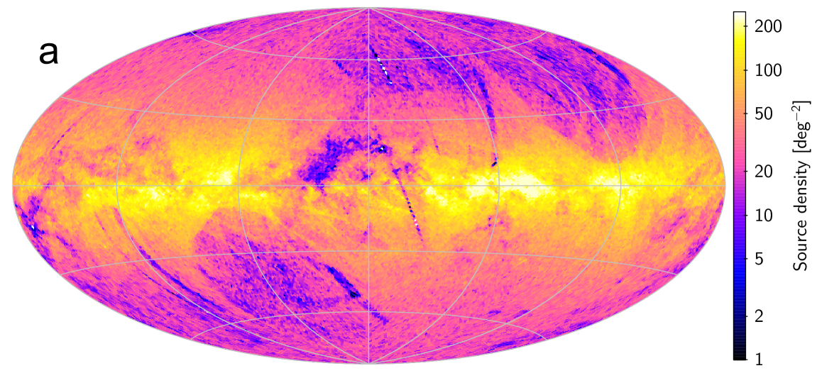
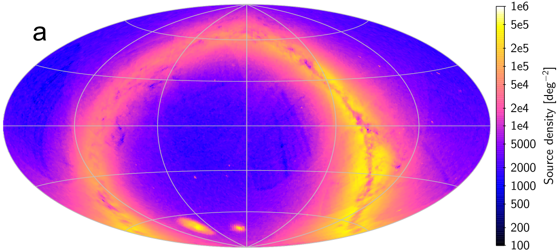
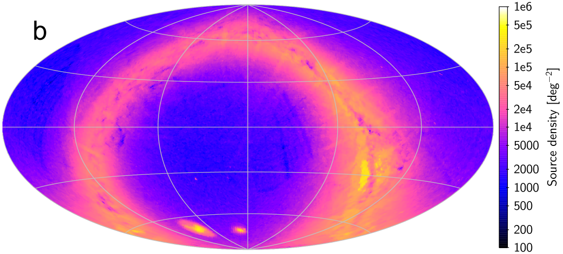
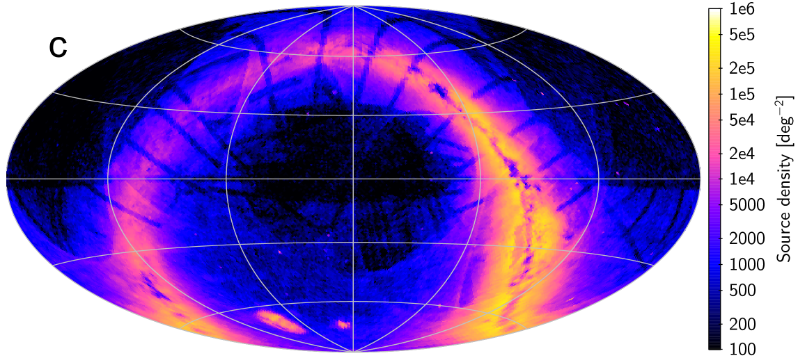
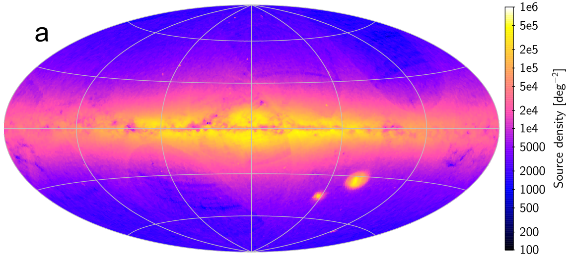
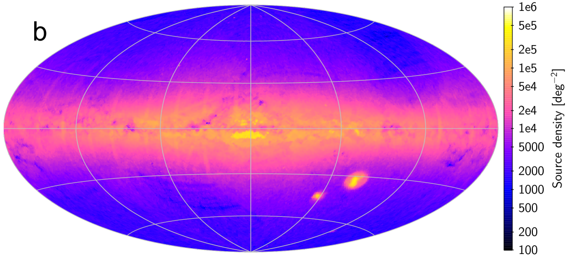
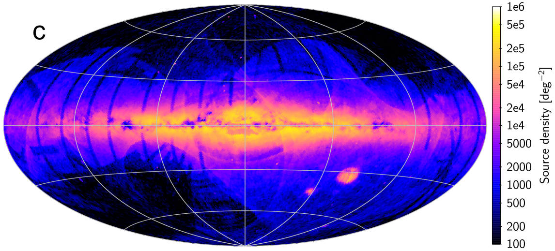
Applying the selection criterion in Eq. (12) results in accepted positional solutions for 1467 million entries, of which 771 million are in the IGSL and 695 million are new sources. A large number of entries in the IGSL were found to be redundant, resulting in nearly coinciding positional solutions. The secondary data set of Gaia DR1 consists of the 1 140 622 719 non-redundant entries that also have valid photometric information. The leftmost maps in Fig. 8 shows the total density of sources in the secondary data set; the other two maps show the densities of the IGSL and new sources. Imprints of the ground-based surveys used in the construction of the IGSL are clearly seen in the latter two maps (as over- and under-densities in Fig. 8b and c, respectively). These are largely absent in the total density map (Fig. 8a), which however still shows features related to the scanning law of Gaia (cf. Fig. 6b). Figure 9 shows the same densities in Galactic coordinates.

The secondary data set contains only positions, with their estimated uncertainties and other statistics, but no parallaxes or proper motions. Some statistics are summarised in Table 2. The standard uncertainties in position are calculated using the recipe in Michalik et al. (2015b). This provides a conservative estimate based on a Galactic model of the distribution of the (neglected) parallaxes and proper motions.

6 Validation

A significant effort has been devoted to examining the quality of the astrometric solutions contributing to Gaia DR1. This validation has been made in two steps, by two independent groups using largely different approaches. The first step, carried out by the AGIS team responsible for the solutions, aimed to characterise the solutions and design suitable filter criteria for the published results. In the second step, carried out by a dedicated data validation team within the Gaia Data Processing and Analysis Consortium (Gaia collaboration, Brown, et al. 2016), a rigorous set of pre-defined tests were applied to the data provided (Arenou et al. 2016).

Only the validation tests performed by the AGIS team on the primary solution and on the auxiliary quasar solution are described here. They are of three kinds:

1. The residuals of the astrometric least-squares solutions were analysed in order to verify that they behave as expected, or alternatively to expose deficiencies in the modelling of the data. See Appendix D.

2. Special TGAS runs were made, in which the modelling of the Gaia instrument or attitude was modified, or different subsets of the observations were used. These are consistency checks of the data, and could also reveal if the results are unduly sensitive to details of the modelling. A direct comparison of the resulting astrometric parameters (in particular the parallaxes) provides a direct quantification of this sensitivity. See Appendix E.

3. The results were compared with independent external data, such as astrometric parameters from the Hipparcos catalogue and expected results for specific astrophysical objects (quasars, cepheids, etc.). See Appendices B and C.

The validation tests were completed before the final selection of sources had been made, and are therefore based on more sources than finally retained in Gaia DR1.

The detailed results of these exercises are given in the appendices. In summary, the comparisons with external data (Appendix B and C) show good agreement on a global level, with differences generally compatible with the stated precisions of the primary data set and of the comparison data. However, there are clear indications of systematic differences at the level of $\pm 0.2$ mas, mainly depending on colour and position on the sky. Such differences may extend over tens of degrees (Figs. 31–32). Very locally, even larger systematics are indicated, which would affect a small fraction of the sources. The statistical distributions of the differences typically have Gaussian-like cores with extended tails including outliers. The analysis of residuals (Appendix D) allows us to identify important contributors to the random and systematic errors, i.e. attitude modelling errors (including micro-clanks and micrometeoroid hits) and colour-dependent image shifts in the optical instrument (chromaticity). The special validation solutions (Appendix E) confirm these findings and provide some quantification of the resulting errors, while pointing out directions for future improvements.

7 Known problems: Causes and cures

The preliminary nature of the astrometric data contained in Gaia DR1 cannot be too strongly emphasised. TGAS has allowed us to develop our understanding of the instrument, exercise the complex data analysis systems, and obtain astrophysically valuable results in a much shorter time than originally foreseen. This has been possible thanks to a number of simplifications and shortcuts, which inevitably weakens the solution in many respects. Additional weaknesses have been identified during the validation process (Appendix E), and more will undoubtedly be discovered by users of the data.

Importantly, the weaknesses identified so far are either an expected consequence of the imposed limitations of Gaia DR1, or of a character that will be remedied by the planned future improvements of the data analysis. The most important known weaknesses, and their remedies, are listed below.

1. Limited input data: the data sets are based on a limited time interval – less than a quarter of the nominal mission length. The primary astrometric solution, providing the attitude and calibration parameters, uses less than 1% of the data volume expected for the final astrometric solution. Both the length of the observed interval and the number of primary sources used in the astrometric solution will increase with successive releases.

2. Prior data: the use of prior positional information from the Hipparcos and Tycho-2 catalogues limits the primary data set to a few million of the brightest stars ($\lesssim 11.5$ mag). These are in many ways the most problematic ones because of CCD gating, partially saturated images, etc. Moreover, the positional errors in these catalogues affect the resulting proper motions and parallaxes. Future releases will not use any prior astrometric information at all, except for aligning the reference frame.

3. Cyclic processing: the astrometric solution is designed to be part of a bigger processing loop, including the gradual refinement of the calibration of LSF and PSF versus the spectral energy distribution of the sources. For Gaia DR1 this loop had not been closed, and the centroiding was done against a bootstrap library prepared pre-launch using the limited knowledge of the instrument at the time. The image centroids used for the present solutions are therefore strongly affected by chromaticity and other uncalibrated variations of the LSF and PSF. The effect of this is clearly seen both in the residuals (Appendix D.2) and in the astrometric data (Appendix E). For the next data release the loop will have been closed and executed once, which should drastically reduce some of these effects. The final astrometric solution will be based on several cyclic processing loops, which should almost completely eliminate the centroid errors caused by systematic variations of the LSF and PSF, including chromaticity.

4. Cross-matching: the cross-matching of Gaia observations to sources is far from perfect owing to the use of crude estimates of the attitude and calibration, and an initial source list compiled mainly from ground-based data. The lack of stars with high proper motion ($\mu>3.5$ arcsec yr^-1) in Gaia DR1 is one unfortunate consequence. The astrometric solutions for subsequent releases will be based on the much improved cross-matchings made as part of the cyclic processing loop mentioned above. The final list of sources detected and observed by Gaia will be independent of ground-based surveys.

5. Attitude model: The relatively low density of sources in the primary solution ($\sim$10 deg^-2 in large parts of the sky; see Fig. 5a) required the use of a longer knot interval (30 s) for the attitude model than foreseen in the final astrometric solution ($<$ 10 s; see the AGIS paper, Sect. 7.2.3, and Risquez et al. 2013). Residual modelling errors contribute significant correlated noise in the present solution. This will be eliminated by the vastly improved attitude modelling made possible by a much higher density of primary sources.

6. Micro-clanks and micrometeoroid hits: these are not treated at all, or only by placing gaps around major micrometeoroid hits. Micro-clanks are much more frequent than expected from pre-launch estimates, and could be a major contribution to the attitude modelling errors even for very short knot intervals, if not properly handled. The use of rate data (estimates of the spacecraft angular velocity that do not require AGIS) to detect and quantify micro-clanks was not foreseen before the commissioning of Gaia, but has emerged as an extremely efficient way to eliminate the detrimental effect of micro-clanks (Appendix D.4). For future data releases this will be implemented, and a similar technique can be used to mitigate the effects of small micrometeoroid hits and other high-frequency attitude irregularities.

7. Source model: all sources are treated as single stars, and the radial component of their motions is ignored. Thus, all variations in proper motion due to orbital motion in binaries or perspective effects are neglected. The proper motions given are the mean proper motions between the Hipparcos/Tycho epoch (around J1991.25) and the Gaia DR1 epoch (J2015.0). For resolved binaries, it could be that the positions at the two epochs are inconsistent, e.g. referring to different components, or to one of the components at one epoch, and to the photocentre at the other.

8. Calibration model: the geometric instrument calibration model used for the current primary solution does not include the full range of dependencies foreseen in the final version. This concerns in particular the small-scale irregularities, i.e. the small AL displacements from one pixel column to the next, and their dependence on the gate and time. Moreover, the large-scale calibration parameters evolve too quickly for the currently used time resolution (see Fig. 10). These issues can be resolved by better adapting the model to the observed variations, for example by using polynomial segments or splines for their temporal evolution.

9. Basic-angle variations: for this data release, basic-angle variations have been corrected by simply adopting the (smoothed) variations measured by the BAM (Appendix A.2). We know from simulations that a very wide range of basic-angle variations (depending on their frequency and other characteristics) can in fact be calibrated as part of the astrometric solution. Special validation solutions, which include the harmonic coefficients of the basic angle variations as unknowns, show that this is indeed possible for variations of the kind seen in actual data. It is expected that future astrometric solutions will have the basic-angle variations largely determined by such self-consistent calibrations rather than relying on BAM data. The latter will still be important as an independent check and for detecting basic-angle jumps and other high-frequency features.

10. Spatially correlated systematics: Several of the weaknesses mentioned above combine to produce systematic errors that are strongly correlated over areas that may extend over tens of degrees. Such errors are not much reduced by averaging over any number of stars in a limited area, e.g. when calculating the mean parallax or mean proper motion of a stellar cluster. This will greatly improve in future releases of Gaia data thanks to the generally improved modelling of the instrument and attitude.

With such a long list of problems and weaknesses identified in the data already before their release, one might wonder if the release should not have been postponed until a number of these issues have been fixed or mitigated. However, we believe that the current results are immensely valuable in spite of these problems, provided that the users are aware of them. Moreover, future improvements of the data analysis can only benefit from experiences gained in the early astrophysical use of the data.

8 Conclusions

The inclusion of positional information from the Hipparcos and Tycho-2 catalogues in the early Gaia data processing has allowed us to derive positions, parallaxes, and proper motions for about 2 million sources from the first 14 months of observations obtained in the operational phase of Gaia. This primary data set contains mainly stars brighter than $V\simeq 11.5$. In a secondary data set, using the attitude and geometric calibration of Gaia’s instrument obtained in the primary solution, approximate positions have been derived for an additional 1141 million sources down to the faint limit of Gaia ($G\simeq 20.7$).

All positions are given in the ICRS and refer to the epoch J2015.0. For the primary data set, the overall alignment of the positions with the extragalactic radio frame (ICRF2) is expected to be accurate to about 0.1 mas in each axis at the reference epoch. The proper motion system is expected to be non-rotating with respect to the ICRF2 to within 0.03 mas yr^-1. The positional reference frame of Gaia DR1 coincides with the Hipparcos reference frame at epoch J1991.25, but the Hipparcos frame is rotating with respect to the Gaia DR1 frame by about 0.24 mas yr^-1 (and hence with respect to ICRF by a similar amount). The median uncertainty of individual proper motions is 0.07 mas yr^-1 for the Hipparcos stars and 1.4 mas yr^-1 for non-Hipparcos Tycho-2 stars. The derived proper motions represent the mean motions of the stars between the two epochs J1991.25 and J2015.0, rather than their instantaneous proper motions at J2015.0.

The trigonometric parallaxes derived for the primary data set have a median standard uncertainty of about 0.32 mas. This refers to the random errors. Systematic errors, depending mainly on position and colour, could exist at a typical level of $\pm 0.3$ mas. This includes a possible global offset of the parallax zero point by $\pm 0.1$ mas, and the regional (spatially correlated) and colour-dependent systematics of $\pm 0.2$ mas revealed by the special validation solutions described in Appendix E. These systematics cannot be much reduced by averaging over a number of stars in a small area, such as in a stellar cluster.

The many solutions and validation experiments leading up to the Gaia DR1 data sets have vastly expanded our understanding of Gaia’s astrometric behaviour and boosted our confidence that Gaia will in the end provide results of extraordinary quality. Meanwhile, users of Gaia DR1 data should be extremely aware of the preliminary nature of the current results, and of the various deficiencies discussed in this paper, as well as the potential existence of other yet undetected issues.

Appendix A Geometric calibration of the Gaia instrument

This appendix gives some details on the instrument calibration model used in the current astrometric solutions and presents selected results on some key calibration parameters. It also explains how the BAM data were used to correct the observations.

A.1 Calibration parameters estimated in the astrometric solution

The instrument calibration model is both an extension and simplification of the one described by Eqs. (15)–(18) in Sect. 3.4 of the AGIS paper (Lindegren et al. 2012). The model consists of a nominal part, a constant part, and a time-dependent part. For the AL component it can be written

$$\eta_{fngw}(\mu,\,t)=\eta^{0}_{ng}(\mu)+\Delta\eta_{fngw}(\mu)+\Delta\eta_{fn}(\mu,\,t)\,,$$ (13)

where $\mu$ is the AC pixel coordinate (running from 13.5 to 1979.5 across the CCD columns) and $t$ is time; $\eta^{0}_{ng}$ is the nominal geometry depending on the CCD (index $n$) and gate ($g$) used; $\Delta\eta_{fngw}$ is the constant part depending also on the field index ($f$) and window class ($w$, see footnote 1); and $\Delta\eta_{fn}$ is the time-dependent part. The dependence on $\mu$ (within a CCD) and/or $t$ (within a calibration interval) is written as a linear combination of shifted Legendre polynomials $L^{*}_{l}(x)$, orthogonal on $[0,\,1]$ and reaching $\pm 1$ at the end points, i.e. $L^{*}_{0}(x)=1$, $L^{*}_{1}(x)=2x-1$, and $L^{*}_{2}(x)=6x^{2}-6x+1$.

In the current AL calibration model, the constant part is decomposed as

$$\Delta\eta_{fngw}(\mu)=\sum_{l=0}^{2}\Delta\eta^{\text{g}}_{lfng}L^{*}_{l}(\tilde{\mu})+\sum_{l=0}^{2}\Delta\eta^{\text{w}}_{lfnw}L^{*}_{l}(\tilde{\mu})+\sum_{l=0}^{1}\Delta\eta^{\text{b}}_{lfnb}L^{*}_{l}(\overline{\mu}_{b})\,,$$ (14)

where the superscripted constants are the calibration parameters and $\tilde{\mu}=(\mu-13.5)/1966$ is the normalised AC pixel coordinate. The dependence on CCD gate (superscript “g”) is different in the preceding and following field of view, caused by the slightly different effective focal lengths; hence $\Delta\eta^{\text{g}}$ must depend on the field index $f$. The effect of the window class (“w”) could also depend on $f$, and similarly the third term (“b”) in Eq. (14), which represents the intermediate-scale irregularities of the CCD that cannot be modelled by a polynomial over the full AC extent of the CCD. In practice the medium-scale irregularities are largely associated with the discrete stitch blocks resulting from the CCD manufacturing process (Gaia collaboration, Prusti, et al. 2016). The stitch blocks are 250 pixel columns wide, except for the two outermost blocks which are 108 columns wide; the exact block boundaries are therefore $\mu=13.5$, $121.5$, $371.5$, $\dots$, $1621.5$, $1871.5$, $1979.5$. The intermediate-scale errors are here modelled by a separate linear polynomial for each stitch block, depending on the block index $b=\lfloor(\mu+128.5)/250\rfloor$ and the normalised intra-block pixel coordinate $\overline{\mu}_{b}=(\mu-\mu_{b})/(\mu_{b+1}-\mu_{b})$. Here, $[\mu_{b},\,\mu_{b+1}]$ are the block boundaries given above for $b=0\dots 8$. Small-scale irregularities, which vary on a scale of one or a few CCD pixel columns, are clearly present but not modelled in the current solution.

Figure 10: Evolution of selected calibration parameters estimated in the primary solution. Time is expressed in revolutions of the onboard mission timeline (OBMT; Sect. 3.1). Vertical grey lines indicate the breakpoints $t_{j}$ of the calibration model. Top: basic-angle offset, Eq. (17), with a zoom to the final $\sim$100 revolutions. Bottom: parameter $\Delta\eta^{(0)}_{1fnj}$, representing a small rotation of the CCD in its own plane, for the nine CCDs in row 3. Colours violet to brown are used for AF1 to AF9 (see Fig. 1), respectively.

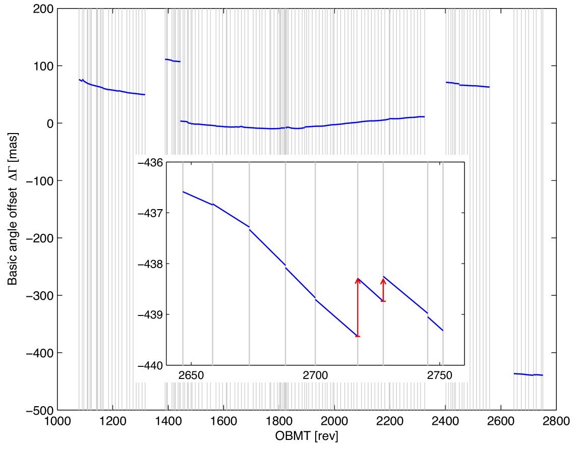
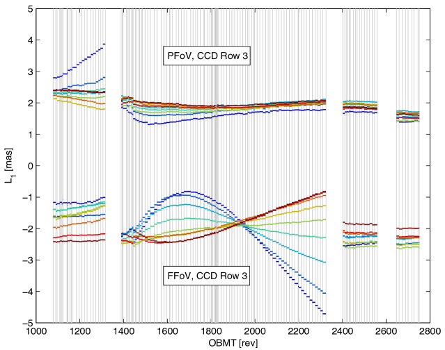
The time-dependent part of the AL calibration needs to take into account the joint dependence on $\mu$ and $t$, which quite generally can be expanded in terms of the products of one-dimensional basis functions. With $\tilde{t}_{j}=(t-t_{j})/(t_{j+1}-t_{j})$ denoting the normalised time coordinate in calibration interval $j$, we have

$$\Delta\eta_{fn}(\mu,\,t)=\sum_{l=0}^{L}\sum_{m=0}^{M_{l}}\Delta\eta^{(m)}_{lfnj}L^{*}_{l}(\tilde{\mu})L^{*}_{m}(\tilde{t}_{j})\,,$$ (15)

where $L$ is the maximum degree of the polynomial in $\mu$ and $M_{l}$ is the maximum degree of the polynomial in $t$ that is combined with a polynomial in $\mu$ of degree $l$. The current model uses $L=2$, as for the constant part, and $M_{0}=1$, $M_{1}=M_{2}=0$; thus Eq. (15) simplifies to

$$\Delta\eta_{fn}(\mu,\,t)=\sum_{l=0}^{2}\Delta\eta^{(0)}_{lfnj}L^{*}_{l}(\tilde{\mu})+\Delta\eta^{(1)}_{0fnj}L^{*}_{1}(\tilde{t}_{j})\,.$$ (16)

In analogy with Eq. (19) in the AGIS paper, the basic-angle offset can be computed from the calibration parameters as

$$\Delta\Gamma(t)=\frac{1}{62}\sum_{n\in\text{AF}}\sum_{f}\left(\Delta\eta^{(0)}_{0fnj}+\Delta\eta^{(1)}_{0fnj}L^{*}_{1}(\tilde{t}_{j})\right)f\,,$$ (17)

where $f=\pm 1$ for the preceding and following field of view, respectively. In the present model this function is piecewise linear as illustrated in the top panel of Fig. 10.

Table 3: Number of parameters of different kinds in the geometric calibration model used for Gaia DR1.

Kind of	Multiplicity							Total
parameter	$l$	$f$	$n$	$g$	$b$	$w$	$j$/$k$	number
$\Delta\eta^{(0)}_{lfnj}$	3	2	62	1	1	1	141	52 452
$\Delta\eta^{(1)}_{lfnj}$	1	2	62	1	1	1	141	17 484
$\Delta\eta^{\text{g}}_{lfng}$	3	2	62	9	1	1	1	3 348
$\Delta\eta^{\text{b}}_{lfnb}$	2	2	62	1	9	1	1	2 232
$\Delta\eta^{\text{w}}_{lnw}$	3	2	62	1	1	3	1	1 116
$\Delta\zeta^{\,(0)}_{lfnk}$	3	2	62	1	1	1	87	32 364
$\Delta\zeta^{\,(1)}_{lfnk}$	1	2	62	1	1	1	87	10 788
$\Delta\zeta^{\text{\,b}}_{lfng}$	3	2	62	9	1	1	1	3 348

For the AC calibration we have in analogy with Eq. (13)

$$\zeta_{fng}(\mu,\,t)=\zeta^{\,0}_{fn}(\mu)+\Delta\zeta_{fng}(\mu)+\Delta\zeta_{fn}(\mu,\,t)\,.$$ (18)

The AC model has fewer breakpoints for the time dependence, no dependence on window class, and no intermediate or small-scale irregularities. Thus,

$$\Delta\zeta_{fng}(\mu) =\sum_{l=0}^{2}\Delta\zeta^{\text{\,b}}_{lfng}L^{*}_{l}(\tilde{\mu})$$ (19)

$$\Delta\zeta_{fn}(\mu,\,t) =\sum_{l=0}^{2}\Delta\zeta^{\,(0)}_{lfnk}L^{*}_{l}(\tilde{\mu})+\Delta\zeta^{\,(1)}_{0fnk}L^{*}_{1}(\tilde{t}_{k})\,,$$ (20)

where $\tilde{t}_{k}=(t-t_{k})/(t_{k+1}-t_{k})$ are normalised time coordinates relative to the breakpoints $t_{k}$ for the AC calibration time intervals.

The calibration model does not include colour- or magnitude-dependent terms, although such dependencies can be expected from chromaticity and non-linear charge transfer inefficiency in the CCDs. Chromatic effects are indeed apparent in the residuals, and will have an effect on the astrometric results as discussed in Appendix E.1.

The model as described applies to the 62 CCDs in the AF; for the SM the nominal calibration $\eta^{0}_{ng}(\mu)$, $\eta^{0}_{ng}(\mu)$ is not updated in the current solution as the SM observations are not used for the astrometric solution in this release.

Table 3 summarises the number of parameters of the different kinds. The total number of calibration parameters is 76 632 for the AL model and 46 500 for the AC model. The calibration model as described above is degenerate because it does not specify a unique division between the different components. For example, the parameter $\Delta\eta^{(0)}_{0fnj}$, averaged over all calibration intervals $j$, describes an AL offset of CCD $n$ in field $f$ that is independent of $\mu$; but $\Delta\eta^{\text{b}}_{0fnb}$ could describe exactly the same offset by means of a constant value for all stitch blocks $b$. In the solution a number of constraints are imposed on the calibration parameters, which make them non-degenerate with each other and with the attitude model. These constraints are essentially the same as Eqs. (16)–(18) in the AGIS paper and not repeated here.

A few examples of calibration results are shown in Fig. 10. The top panel shows the long-term evolution of the basic-angle offset $\Delta\Gamma$. Major discontinuities between the continuous segments are usually real; two examples are shown in the inset diagram where the red arrows show the sizes of jumps determined from BAM data at two of the breakpoints. Refocusing and decontamination cause much larger jumps. The bottom panel shows the evolution of the coefficient of $L^{*}_{1}(\tilde{t}_{j})$ in Eq. (16) for selected CCDs in both fields of view. This parameter represents a small, apparent rotation of the CCD in its own plane, caused mainly by the optical distortion. Between refocusing and decontamination events, this parameter varies smoothly over time and according to position (CCD) in the field, but very differently in the two fields of view. Plots such as these, showing a generally smooth development of calibration parameters from one discrete time interval to the next, suggest that the adopted geometric calibration model is physically sound and adequate at a precision level better than 0.1 mas.

A.2 Calibration parameters derived from BAM data

The periodic variations seen in the BAM signal are strongly coupled to the spin phase of the satellite with respect to the Sun. The heliotropic spin phase $\Omega$ increases by $360^{\circ}$ for each $\sim$6 hr spin period and is zero when the direction to the apparent Sun is symmetrically located between the two fields of view (see Fig. 1 in Michalik & Lindegren 2016). Figure 11 shows an example of the line-of-sight variations in the preceding field of view during a one-day interval (four successive spin periods). In such a time interval, and for a given field of view (P or F), the following model was usually found to provide a reasonable fit to the line-of-sight variations, as represented by the location $\xi$ (expressed as an angle) of the central fringe on the BAM CCD:

$$\xi^{\text{P}}(t)=C^{\text{P}}_{0}+(t-t_{0}){C^{\prime}_{0}}^{\text{P}}+\sum_{k=1}^{8}\Bigl{[}C_{k}^{\text{P}}\cos k\Omega(t)+S_{k}^{\text{P}}\sin k\Omega(t)\Bigr{]}\,,$$ (21)

with a similar expression for $\xi^{\text{F}}(t)$ in the other field of view. Here $t_{0}$ is the mid-time of the interval and $C^{\text{P}}_{0}$, ${C^{\prime}}^{\text{P}}_{0}$, $C^{\text{P}}_{k}$, and $S^{\text{P}}_{k}$ ($k=1,\,\dots,\,8$) are constants in the interval. Detected discontinuities were subtracted before fitting this model. Residuals of the fit are typically on the level of a few tens of $\mu$as and contain systematic patterns (e.g. as seen in the lower panel of Fig. 11) that correlate with spacecraft activities such as changes in the telemetry rates. The constant and linear coefficients $C^{\text{P}}_{0}$ and ${C^{\prime}_{0}}^{\text{P}}$ are not further used in the analysis.

Fits using Eq. (21) were made independently for the preceding (P) and following (F) fields of view, resulting in two sets of harmonic coefficients for each fitted time interval. The differences between these, in the sense F minus P, provide a corresponding harmonic representation of the basic-angle variations:

$$\Delta\Gamma(t)=\sum_{k=1}^{8}\Bigl{[}C_{k}\cos k\Omega(t)+S_{k}\sin k\Omega(t)\Bigr{]}\,,$$ (22)

with a separate estimate of $C_{k}=C^{\text{F}}_{k}-C^{\text{P}}_{k}$ and $S_{k}=S^{\text{F}}_{k}-S^{\text{P}}_{k}$ ($k=1\dots 8$) obtained for each one-day interval.

The sizes of the harmonic coefficients $C_{k}$, $S_{k}$ decrease rapidly with increasing order $k$ (Table 6). The harmonic coefficients are only approximately constant over the investigated 14 months of BAM data. At least three different kinds of variations can be distinguished: (i) an annual periodic variation; (ii) a secular trend; and (iii) seemingly more irregular, rapid variations on timescales of weeks to months.

The annual and secular variations are well fitted by the following analytical model, in which each coefficient is approximated as a linear function modulated by the expected inverse-square dependence on solar distance:

$$C_{k}(t)=\Bigl{[}C_{k,0}+(t-t_{\text{ref}})C_{k,1}\Bigr{]}\times d(t)^{-2}\,,\quad k=1\dots 8\,$$ (23)

(and similarly for $S_{k}$). Here $t_{\text{ref}}=\text{J2015.0}$ and $d(t)$ is Gaia’s heliocentric distance in au. This analytical fit was used to correct the observations for the basic angle variations in the astrometric solutions for Gaia DR1.

The temporal evolution of the dominant first order ($k=1$) is shown in Fig. 12, where the Fourier coefficients have been transformed to amplitude $A_{1}$ and phase $\phi_{1}$ such that $C_{1}=A_{1}\cos\phi_{1}$ and $S_{1}=A_{1}\sin\phi_{1}$. The fitted Eq. (23) is shown by the red solid curves. In addition to the annual variation of $\pm 3.3$% in amplitude, caused by the eccentricity of Gaia’s heliocentric orbit, the plots show secular trends in both amplitude and phase at the level of several percent, as well as systematic deviations from the model in Eq. (23). At least some of these deviations are related to the mean rate of observations. At the time of writing it is not clear if they represent actual changes in the basic-angle variations, or if they are merely an artefact of the BAM. Until this has been established, the smoothed model in Eq. (23) is used to correct the observations.

Figure 11: Example of the BAM signal for the preceding field of view. Time is expressed in revolutions of the onboard mission timeline (OBMT; Sect. 3.1). Top: individual fringe position measurements $\xi^{\text{P}}$ after removal of outliers. Bottom: residuals after fitting the model in Eq. (21).

Figure 12: Amplitude ($A_{1}$) and phase ($\phi_{1}$) of the first harmonic in Eq. (22) fitted to the BAM signal. Time is expressed in revolutions of the onboard mission timeline (OBMT; Sect. 3.1). Circles are the values for individual one-day intervals; the solid curve is the global model used to correct the observations in Gaia DR1. The vertical dashed lines mark the two major data gaps caused by decontamination procedures.

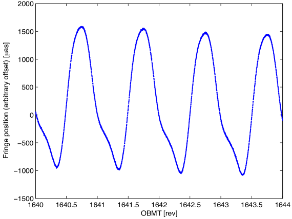
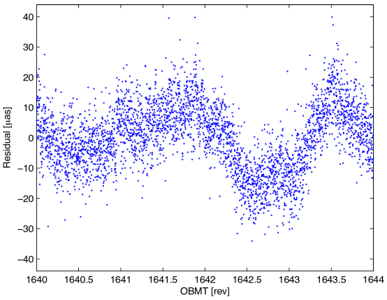
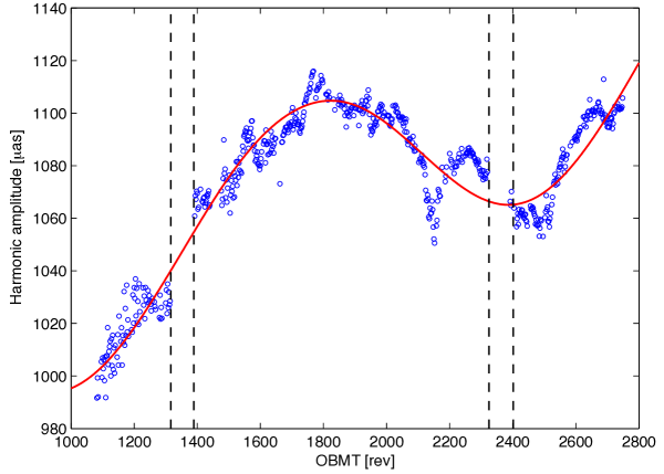
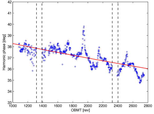
Appendix B Estimating the precision of parallaxes from a comparison with Hipparcos data

In this appendix we describe how the external uncertainties of the TGAS parallaxes were estimated based on a comparison with Hipparcos data. These estimates were used to calculate the inflation factor in Eq. (4) applied to all formal uncertainties in the primary data set of Gaia DR1.

In AGIS the least-squares estimates of the astrometric parameters are rigorously computed in the iterative solution, but the associated uncertainties are only approximately estimated, using a number of simplifications. For a given source, the formal standard errors (uncertainties) of the five astrometric parameters are computed as described in Sect. 6.3 of the AGIS paper, i.e. from the diagonal elements of the inverse of the corresponding $5\times 5$ part of the normal matrix. As discussed by Holl & Lindegren (2012) this neglects the statistical correlations introduced by the attitude and calibration models, which couple the observation equations of different sources to each other. This will cause the actual uncertainties to be underestimated. In Gaia DR1 the underestimation may be particularly severe because of the large modelling errors and relatively low redundancy of observations. It is therefore important to investigate the relation between the formal standard uncertainties computed from the least-squares solution, here denoted by $\varsigma$, and the actual standard uncertainties, denoted by $\sigma$. (The word standard here signifies that the quantities represent standard deviations. It does not imply that the errors follow, or even are assumed to follow, the normal distribution. For the subsequent derivation it is sufficient to assume that the errors have finite variance.)

A comparison of the Hipparcos parallaxes with the corresponding values from the current primary (TGAS) solution offers an interesting possibility to investigate this relation, thanks to the following circumstances: (i) the parallax errors in the two data sets are uncorrelated, since the Hipparcos parallaxes were not used in the solution (Michalik et al. 2015a); (ii) the standard uncertainties do not differ too much between the two data sets; and (iii) the number of common stars is large enough for accurate statistics.

For the comparison we use the parallaxes (and their uncertainties) from the new reduction of the Hipparcos data (van Leeuwen 2007a). The primary solution, after application of the filter in Eq. (11), contains data for 101 106 Hipparcos stars that were used for the present study, although not all of them are retained in Gaia DR1. The two sets of parallax values are here distinguished by subscript H (for Hipparcos) and T (for TGAS). For the stars in common the median formal uncertainty is $\varsigma_{\text{H}}\simeq 0.9$ mas for the Hipparcos parallaxes and $\varsigma_{\text{T}}\simeq 0.15$ mas for the TGAS parallaxes.

The non-correlation between the two sets of parallaxes implies that the variance of $\Delta\varpi=\varpi_{\text{T}}-\varpi_{\text{H}}$ equals the sum of the actual mean variances,

$$\text{Var}(\Delta\varpi)=\langle\sigma_{\text{T}}^{2}\rangle+\langle\sigma_{\text{H}}^{2}\rangle\,.$$ (24)

The angular brackets denote averages over the stars, which is necessary in order to take into account the non-uniformity (heteroscedasticity) of the data sets. $\text{Var}(\Delta\varpi)$ is readily estimated, e.g. as the sample variance of the parallax differences, and thus provides a firm estimate of the combined mean variances of the data sets. This should be compared with the combined formal variances,

$$\langle\varsigma_{\Delta\varpi}^{2}\rangle=\langle\varsigma_{\text{T}}^{2}\rangle+\langle\varsigma_{\text{H}}^{2}\rangle\,.$$ (25)

Consider for example the $\simeq\,$86 000 stars with formal parallax standard uncertainties $\varsigma_{\text{T}}\leq 0.7$ mas and $\varsigma_{\text{H}}\leq 1.5$ mas. The rms formal standard uncertainties are $\langle\varsigma_{\text{T}}^{2}\rangle^{1/2}=0.226$ mas and $\langle\varsigma_{\text{H}}^{2}\rangle^{1/2}=0.915$ mas, giving a combined standard deviation $\langle\varsigma_{\Delta\varpi}^{2}\rangle^{1/2}=0.942$ mas. However, the sample standard deviation of $\Delta\varpi$ is 1.218 mas (excluding nine stars for which $|\Delta\varpi|>10$ mas). From this we conclude that $\varsigma_{\text{T}}$ and/or $\varsigma_{\text{H}}$ significantly underestimate the true errors. This analysis can be repeated for various selections of formal uncertainties, providing in each case an estimate of the combined uncertainties.

However, as shown below, it is also possible to estimate the relative contributions of the data set to the combined variance, and hence the variance of each data set separately. The method depends on the practical circumstance that the probability density function of the true parallaxes has a steep edge towards small values.

Let $\varpi\geq 0$ denote the true parallax of a star and $e_{\text{H}}=\varpi_{\text{H}}-\varpi$, $e_{\text{T}}=\varpi_{\text{T}}-\varpi$ the measurement errors in the two data sets. Let us first assume that the measurements are unbiased, $\text{E}(e_{\text{T}})=\text{E}(e_{\text{H}})=0$, where E is the expectation or mean value. The non-correlation assumption is

$$\text{E}(e_{\text{T}}e_{\text{H}})=0\,,$$ (26)

which results in

$$\sigma_{\Delta\varpi}^{2}=\text{E}[(e_{\text{T}}-e_{\text{H}})^{2}]=\text{E}(e_{\text{T}}^{2})+\text{E}(e_{\text{H}}^{2})=\langle\sigma_{\text{T}}^{2}\rangle+\langle\sigma_{\text{H}}^{2}\rangle\,,$$ (27)

which is Eq. (24). Consider now the weighted mean parallax,

$$\varpi_{x}=(1-x)\varpi_{\text{T}}+x\varpi_{\text{H}}\,$$ (28)

for $0\leq x\leq 1$. The error of $\varpi_{x}$ is $e_{x}=(1-x)e_{\text{T}}+xe_{\text{H}}$, and its covariance with $\Delta\varpi$ is

$$\text{Cov}(e_{x},\,\Delta\varpi)=\text{E}[e_{x}(e_{\text{T}}-e_{\text{H}})]=(1-x)\langle\sigma_{\text{T}}^{2}\rangle-x\langle\sigma_{\text{H}}^{2}\rangle\,.$$ (29)

This is clearly zero if 

$$x=\frac{\langle\sigma_{\text{T}}^{2}\rangle}{\langle\sigma_{\text{T}}^{2}\rangle+\langle\sigma_{\text{H}}^{2}\rangle}\,.$$ (30)

Since this holds for any value of the true parallax $\varpi$, it follows that also the covariance between $\varpi_{x}$ and $\Delta\varpi$ is zero for this value of $x$, provided that the errors are not correlated with $\varpi$, which is a reasonable assumption based on how parallaxes are computed.

If therefore $\Delta\varpi=\varpi_{\text{T}}-\varpi_{\text{H}}$ is plotted against $\varpi_{x}$, and $x$ is adjusted for zero correlation between the plotted quantities, the mean variances of the data sets can be calculated as

$$\langle\sigma_{\text{T}}^{2}\rangle=x_{0}\sigma^{2}_{\Delta\varpi}\,,\quad\langle\sigma_{\text{H}}^{2}\rangle=(1-x_{0})\sigma^{2}_{\Delta\varpi}\,,$$ (31)

where $x_{0}$ is the value of $x$ for which the correlation is zero. In practice this procedure only works for small enough parallaxes because the correlation is only apparent when the errors cause the measured parallaxes to be scattered into negative values.

Equations (24)–(31) were derived under the assumption that $\varpi_{\text{T}}$ and $\varpi_{\text{H}}$ are unbiased. However, it is easily verified that the same relations hold when they are biased, provided that the bias is not a function of $\varpi$. While the difference in bias can be estimated as the mean value of $\Delta\varpi$, it is not possible to separate out the bias of each data set with this method.

Figure 13: Parallax difference between TGAS and Hipparcos plotted against the weighted mean parallax (Eq. 28) for three different weight factors $x$: (a) $x=0$, i.e. the abscissa is the TGAS parallax; (b) $x=0.1$; and (c) $x=1$, i.e. the abscissa is the Hipparcos parallax. See text for further explanation.

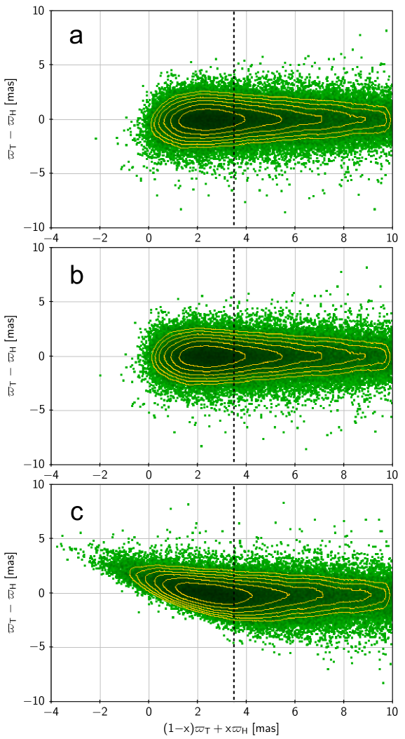
Figure 13 illustrates the application of the method to the previously mentioned selection, $\varsigma_{\text{T}}\leq 0.7$ mas and $\varsigma_{\text{H}}\leq 1.5$ mas. $\Delta\varpi$ is here plotted versus $\varpi_{x}$ for $x=0.0$, 0.1, and 1.0. (Only the $\simeq\,$73 000 points with $\varpi_{x}<10$ mas are shown.) In the top panel (a), the case $x=0$ exhibits a weak positive correlation most clearly seen from the slightly asymmetric distribution of $\Delta\varpi$ for the smallest parallaxes. In the bottom panel (c), the case $x=1$ shows a very strong negative correlation. For $x=0.1$, shown in the middle panel (b), the correlation virtually disappears. Thus we conclude that $x_{0}\simeq 0.1$. With $\sigma_{\Delta\varpi}=1.218$ mas from the sample standard deviation, Eq. (31) gives $\langle\sigma_{\text{T}}^{2}\rangle^{1/2}=0.385$ mas. Comparing with the rms formal uncertainty, $\langle\varsigma_{\text{T}}^{2}\rangle^{1/2}=0.226$ mas, we conclude that the formal parallax uncertainties for this particular sample on the average need to be increased roughly by the inflation factor $F\simeq 1.7$.

In this example $x_{0}$ was estimated by visual inspection of a sequence of $(\varpi_{x},\,\Delta\varpi)$-plots for different values of $x$. It is not difficult to devise an objective and more precise criterion to estimate $x_{0}$ and hence $F$. Let $\rho(\varpi_{x},\Delta\varpi\,|\,x,c)$ denote the sample correlation coefficient between $\varpi_{x}$ and $\Delta\varpi$ calculated for a given value of $x$, using only points with $\varpi_{x}\leq c$, where $c$ is some positive constant. While this sample correlation coefficient in general depends on $c$, we clearly expect $\rho(\varpi_{x},\Delta\varpi\,|\,x_{0},c)=0$ to hold for any value of $c$. Thus, $x_{0}$ can in principle be obtained by solving this equation for arbitrary $c$. In practice we should choose $c$ to minimise the statistical uncertainty of $x_{0}$. Using bootstrap resampling (Efron & Tibshirani 1994) to estimate the uncertainty, it appears that $c=3.5$ mas (dashed line in Fig. 13) is close to optimal, and we find for the three cases in Fig. 13, respectively, $\rho(\varpi_{x},\Delta\varpi\,|\,x,c)=+0.077$, $-0.005$, and $-0.522$ (excluding 13 points for which $|\Delta\varpi|>10$ mas). Estimating $x_{0}$ by bisection we obtain $x_{0}=0.095\pm 0.006$, from which $\langle\sigma_{\text{T}}^{2}\rangle=0.141\pm 0.009$ mas² or $F=1.66\pm 0.05$.

Figure 14: Statistical relation between the formal parallax variances of Hipparcos stars in the primary (TGAS) solution, and the actual variances estimated as described in the text. The solid line is the fitted relation in Eq. (32); the dashed line is the 1:1 relation.

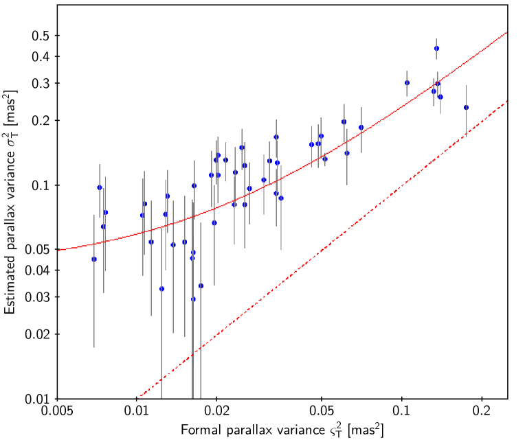
It is not expected that the inflation factor $F$ should be the same for all sources, independent of $\varsigma_{\text{T}}$. To investigate this, the method described above was applied to different subsamples of the data sets, selected according to their formal uncertainties. This makes it possible to trace out the statistical relation between the formal and actual uncertainties. Figure 14 shows the result of such an analysis of the parallaxes in the current primary solution. The estimated mean actual variances $\langle\sigma_{\text{T}}^{2}\rangle$, with 68% confidence limits obtained by bootstrapping, are plotted against the mean formal variances $\langle\varsigma_{\text{T}}^{2}\rangle$ for 49 different subsamples using $c=3.5$ mas and removing points with $|\Delta\varpi|>10$ mas. The solid curve is the relation

$$\langle\sigma_{\text{T}}^{2}\rangle\simeq a^{2}\langle\varsigma_{\text{T}}^{2}\rangle+b^{2}\,$$ (32)

for $a=1.4$ and $b=0.2$ mas, obtained by a weighted least-squares fitting (with some rounding). The adopted inflation factors in Eq. (4) correspond to this curve. The linear form of this relation is mainly empirical, but not without theoretical foundation: neglected correlations tend to give a multiplicative factor to the variance ($a^{2}$), while unmodelled uncorrelated errors add a constant variance ($b^{2}$).

Appendix C Comparison with external data

In this appendix we compare astrometric parameters in the primary (TGAS) solution with some external data of comparable accuracy. The main purpose is to check for possible systematic errors in the primary data set and, if possible, characterise them in terms of their size and dependence on position, colour, etc.

In order to summarise key properties in a few numbers, we generally use robust statistics such as the median for the location of a distribution, and the RSE (see footnote 6) for the scale or dispersion of the distribution. For brevity, the median and RSE of quantity $x$ are denoted by $\text{med}(x)$ and $\text{RSE}(x)$. Where relevant, the standard uncertainty of the median is estimated using bootstrapping (Efron & Tibshirani 1994).

The results of a dedicated validation procedure applied to the Gaia DR1 data are given by Arenou et al. (2016).

Figure 15: Differences in position and parallax between the primary data set (TGAS) and the Hipparcos catalogue for 86 928 sources: (a) difference in right ascension, $(\alpha_{\text{T}}-\alpha_{\text{H}})\cos\delta$; (b) difference in declination, $\delta_{\text{T}}-\delta_{\text{H}}$; (c) difference in parallax, $\varpi_{\text{T}}-\varpi_{\text{H}}$. Median differences at epoch J2015.0 are shown in cells of about 3.36 deg². The position differences have not been corrected for the orientation difference between the Hipparcos reference frame and the reference frame of Gaia DR1. The maps use an Aitoff projection in equatorial (ICRS) coordinates, with origin $\alpha=\delta=0$ at the centre and $\alpha$ increasing from right to left.

Figure 16: Differences in position between the primary data set (TGAS) and the Hipparcos catalogue for 86 928 sources: (a) difference in right ascension, $(\alpha_{\text{T}}-\alpha_{\text{H}})\cos\delta$; (b) difference in declination, $\delta_{\text{T}}-\delta_{\text{H}}$. Median differences at epoch J2015.0 are shown in cells of about 3.36 deg². (c) Number of sources per cell used to compute the median differences here and in Fig. 15. Some empty cells are shown in white. The position differences have been corrected for the orientation difference between the Hipparcos reference frame and the reference frame of Gaia DR1. The maps use an Aitoff projection in equatorial (ICRS) coordinates, with origin $\alpha=\delta=0$ at the centre and $\alpha$ increasing from right to left.

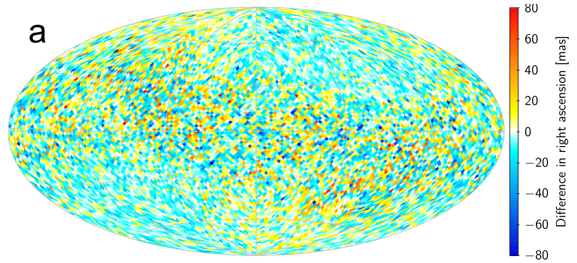
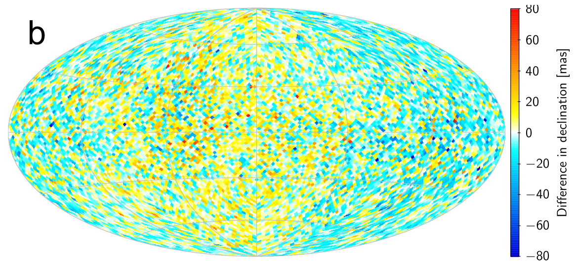
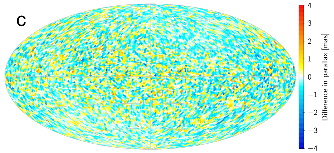
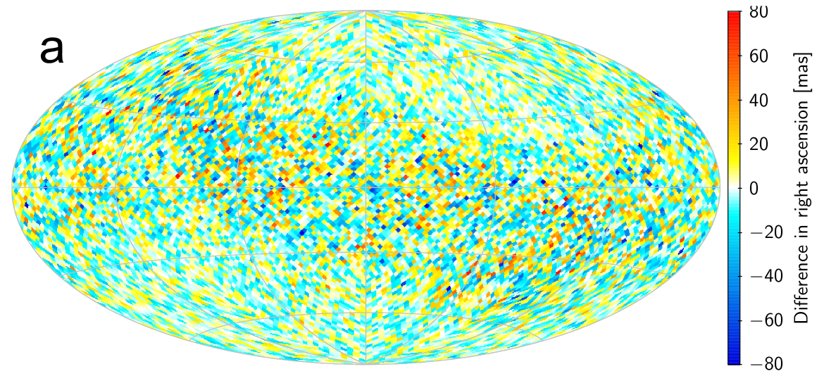
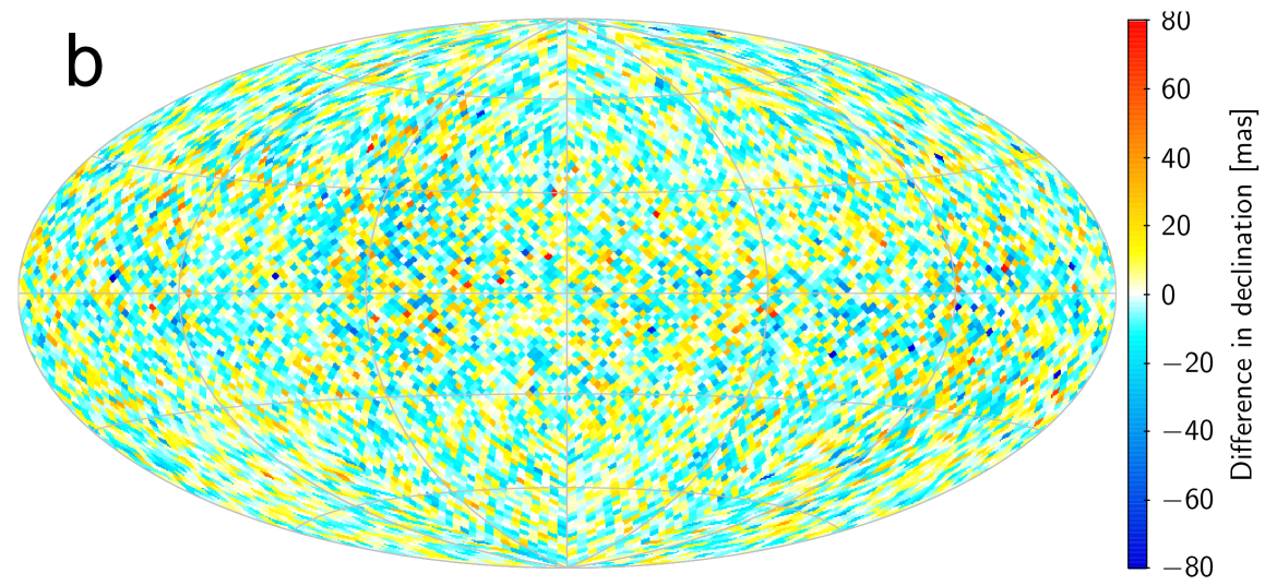
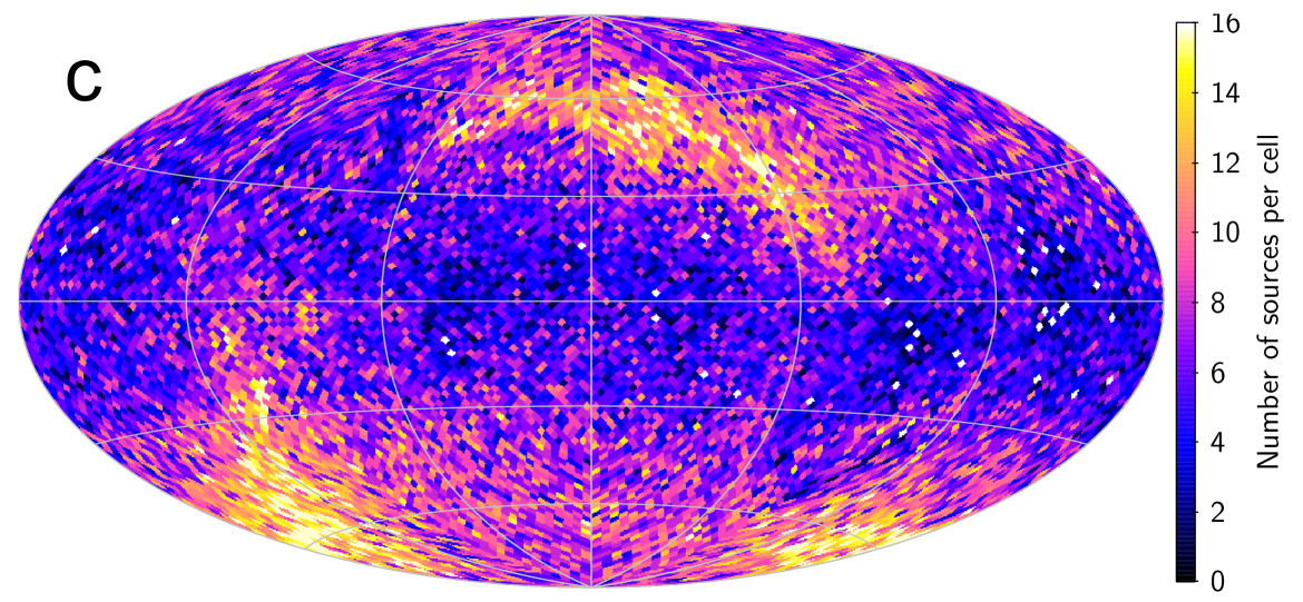
C.1 Comparison with the Hipparcos and Tycho-2 catalogues

The following comparisons are based on the 2 086 766 sources from the primary solution that satisfy Eq. (11), even though not all of them are retained in Gaia DR1. For 101 106 sources with Hipparcos identifiers we compare with the re-reduction of the raw Hipparcos data by van Leeuwen (2007a) as retrieved from the CDS. The Hipparcos astrometric data were propagated to epoch J2015.0 using rigorous formulae (Butkevich & Lindegren 2014), but neglecting light-time and perspective effects by assuming zero radial velocity for all stars. The perspective effect is only relevant for a small number of stars with high proper motion, most of which are missing in Gaia DR1. Unless otherwise specified, the comparison of positions and proper motions is made after rotating the Hipparcos data to the Gaia DR1 frame as explained in Sect. 4.3. Only entries with parallax uncertainty $\leq 1.5$ mas in the Hipparcos catalogue are used for the comparison below, consisting of 86 928 entries in the primary data set. Values from the Hipparcos catalogue are denoted with subscript H, those from the primary (TGAS) data set by T.

In all comparisons we first consider the global differences, i.e. including all sources irrespective of their position, colour, and other characteristics. It should be kept in mind that the resulting statistics are indeed only valid on a global level. The data are in general very inhomogeneous, and as soon as they are broken down according to position, colour, etc., a much more complex picture emerges with sometimes much stronger systematic differences and locally higher dispersions. In this section we focus on the dependence on position (i.e. regional systematics) and, to some extent, on colour.

Hipparcos positions

The global statistics of the positional differences at J2015.0 are $\text{med}(\Delta\alpha*)=-0.073\pm 0.101$ mas, $\text{med}(\Delta\delta)=+0.154\pm 0.089$ mas, $\text{RSE}(\Delta\alpha*)=27.8$ mas, and $\text{RSE}(\Delta\delta)=24.0$ mas, where $\Delta\alpha*=(\alpha_{\text{T}}-\alpha_{\text{H}})\cos\delta$ and $\Delta\delta=\delta_{\text{T}}-\delta_{\text{H}}$ are the position differences in right ascension and declination. The large RSE values are mainly attributable to the Hipparcos errors propagated to J2015.0, where the Hipparcos positions have rms uncertainties of 21.7 mas ($\sigma_{\alpha*}$) and 18.3 mas ($\sigma_{\delta}$), not accounting for possible non-linear motions caused by binarity, etc.

Panels (a) and (b) in Figs. 15–16 show the median differences in $\alpha$ and $\delta$ broken down according to celestial position. In Fig. 15 the position differences are shown as calculated from the catalogue values; in Fig. 16 they have been corrected for the orientation difference ($\@vec{\varepsilon}$) according to Eq. (6). The tessellation uses a Healpix scheme with 12 285 pixels, giving a pixel size of 3.36 deg². The mean number of sources per pixel is thus eight, but the local number varies significantly as shown in Fig. 16c. The smaller density of stars in the ecliptic region $\left|\,\beta\,\right|\lesssim 45^{\circ}$) is partly inherent in the Hipparcos catalogue, but enhanced by our selection $\sigma_{\varpi\text{H}}\leq 1.5$ mas.

The positional differences in Fig. 15a–b show a clear signature of the $\simeq\,$5.6 mas orientation difference between the Gaia DR1 reference frame and the Hipparcos reference frame at J2015.0. This signature is not visible in Fig. 16a–b, where the Hipparcos positions have been rotated by $\@vec{\varepsilon}$.

The median differences, especially in right ascension, show a markedly larger scatter in the ecliptic region than in other parts of the sky. This is partly explained by the lower number of sources per pixel in that region, but mainly reflects the variation of Hipparcos proper motion uncertainties with ecliptic latitude. The propagated Hipparcos positions are clearly not good enough to validate the TGAS positions on a small scale, but do not indicate any large systematics on a semi-global scale. For example, the median differences computed separately for octants of the celestial sphere differ from the global value by at most 1 mas in $\Delta\alpha*$ and 0.6 mas in $\Delta\delta$. A stricter validation of the TGAS positions is possible by means of VLBI data (Sect. C.4).

Hipparcos proper motions

The global statistics of the proper motion differences, after correcting the Hipparcos values to the Gaia DR1 reference frame, are $\text{med}(\Delta\mu_{\alpha*})=-0.003\pm 0.004$ mas yr^-1, $\text{med}(\Delta\mu_{\delta})=+0.006\pm 0.004$ mas yr^-1, $\text{RSE}(\Delta\mu_{\alpha*})=1.17$ mas yr^-1, and $\text{RSE}(\Delta\mu_{\delta})=1.01$ mas yr^-1, where $\Delta\mu_{\alpha*}=\mu_{\alpha*\text{T}}-\mu_{\alpha*\text{H}}$ and $\Delta\mu_{\delta}=\mu_{\delta\text{T}}-\mu_{\delta\text{H}}$ are the proper motion differences in right ascension and declination. As expected, these values are almost exactly equal to the corresponding position differences divided by the epoch difference of 23.75 yr. The maps of the median proper motion differences are not given here, as they are virtually indistinguishable from the corresponding maps of position differences, if the colour scales of the latter are interpreted as proper motion scales in the range $[-3.4,\,+3.4]$ mas yr^-1 ($\pm 80\leavevmode\nobreak\ \text{mas}/23.75\leavevmode\nobreak\ \text{yr}$).

A related comparison is provided by the statistic $\Delta Q$ defined by Eq. (10). $\Delta Q$ measures the proper motion difference between the primary data set (TGAS) and the Hipparcos catalogue, normalised by the covariances provided in the two catalogues. For genuinely single stars, $\Delta Q$ is expected to have an exponential distribution. Figure 17 shows the relative frequencies of $\Delta Q$ for two samples of the Hipparcos entries: the solid blue curve shows bona fide single stars (91 939 entries without any indication of duplicity in the analysis by van Leeuwen 2007a, i.e. of solution type $\text{Sn}=5$), while the dashed red curve shows the remaining stars (9167 entries with $\text{Sn}\neq 5$). The latter include known binaries, acceleration solutions, etc. For comparison, the black line shows the expected exponential distribution. Both samples show an approximately exponential distribution for small values of $\Delta Q$, albeit with a smaller slope than theoretically expected. This could be an effect of underestimated formal uncertainties in either or both catalogues, or as a real cosmic scatter caused by the fact that most stars are actually non-single. The higher relative frequency of large $\Delta Q$ among sources with $\text{Sn}\neq 5$ confirms the expected sensitivity of $\Delta Q$ to duplicity. The sample of bona fide single stars contains some 50 entries with $\Delta Q>1000$, $\sim$1000 with $\Delta Q>100$, and $\sim$10 000 with $\Delta Q>10$. These are clearly candidates for further investigation.

Figure 17: Relative frequencies of the statistic $\Delta Q$ for two selections of stars in the Hipparcos subset of the primary solution: 91 939 bona fide single stars (solid blue curve) and 9167 other stars (dashed red). The black line is the theoretically expected distribution.

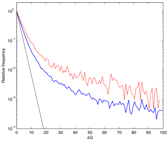
Hipparcos parallaxes

The global statistics of the parallax differences are $\text{med}(\Delta\varpi)=-0.089\pm 0.006$ mas and $\text{RSE}(\Delta\varpi)=1.14$ mas, where $\Delta\varpi=\varpi_{\text{T}}-\varpi_{\text{H}}$. The slightly negative median difference is statistically significant and is clearly seen in a probability density plot of the differences (Fig. 18). The bottom diagram in Fig. 18 shows the distribution of normalised differences $\Delta\varpi/(\sigma_{\varpi\text{T}}^{2}+\sigma_{\varpi\text{H}}^{2})^{1/2}$, using the inflated standard uncertainties $\sigma_{\varpi\text{T}}$ from Eq. (4) and $\sigma_{\varpi\text{H}}$ as given in the Hipparcos catalogue. The distribution is slightly wider than the expected unit normal distribution (the RSE of the normalised parallax differences is 1.22), suggesting that the standard uncertainties are slightly underestimated in one or both data sets. It also displays the non-Gaussian, almost exponential tails often seen in empirical error distributions.

The parallax difference map (Fig. 15c) has many interesting features but we will only comment on a few. The larger scatter in the ecliptic region is obvious, as is the patchiness of the visible structures, suggesting strong spatial correlations on a scale of a few degrees. Both features are expected to be present, to some extent, in both data sets, and it is not possible to conclude from this comparison if they are (mainly) a feature in one or the other data set. Another conspicuous feature is that the northern ecliptic region ($\beta>45^{\circ}$, where $\beta$ is the ecliptic latitude) is on the whole slightly more negative (blue) than the southern ($\beta<-45^{\circ}$). This is confirmed by partitioning the differences according to ecliptic latitude:

$$\text{med}(\Delta\varpi)=\begin{cases}-0.130\pm 0.006\leavevmode\nobreak\ \text{mas}&\text{for $\beta>0$}\,,\\ -0.053\pm 0.006\leavevmode\nobreak\ \text{mas}&\text{for $\beta<0$}\,.\end{cases}$$ (33)

Further analysis reveals that the north–south asymmetry in $\Delta\varpi$ depends on the colour of the star. Subdividing the data according to colour index $V-I$, taken from the Hipparcos catalogue, shows approximately linear trends with opposite signs (Fig. 19) in the two hemispheres. Over the investigated range of colours, the total amplitude of the effect is $\pm 0.1$ mas. While it cannot be excluded that this effect, at least partly, originates from the Hipparcos data, there are strong indications that it is caused by the – as yet uncalibrated – chromaticity of the Gaia instrument (see Appendices C.2, D.2, and E.1).

If the same data are instead subdivided according to magnitude, using $H\!p$ from the Hipparcos catalogue (Fig. 20), there is no clear systematic trend in either hemisphere.

Figure 18: Probability density plots (see footnote 15) of parallax differences, taken in the sense TGAS minus Hipparcos, for a common subset of 86 928 sources. Top: empirical probability density of $\Delta\varpi$ (solid), and for comparison a normal probability density function with standard deviation 1.14 mas (dashed), equal to the RSE of the differences. Bottom: probability density of the normalised parallax differences (solid), and for comparison the unit normal probability density function (see text for details).

Figure 19: Parallax differences (TGAS minus Hipparcos) for 86 928 sources, plotted against colour index. The black line is for northern ecliptic latitudes ($\beta>0$), the grey-white line for southern ($\beta<0$). The lines connect median values calculated in 50 bins subdividing the data according to $V-I$. Each bin contains about 900 data points per hemisphere.

Figure 20: Parallax differences (TGAS minus Hipparcos) for 86 928 sources, plotted against magnitude. The black line is for northern ecliptic latitudes ($\beta>0$), the grey-white line for southern ($\beta<0$). The lines connect median values calculated in 50 bins subdividing the data according to the Hipparcos magnitude $H\!p$. Each bin contains about 900 data points per hemisphere.

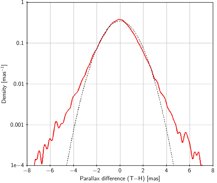
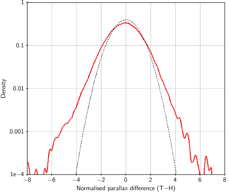
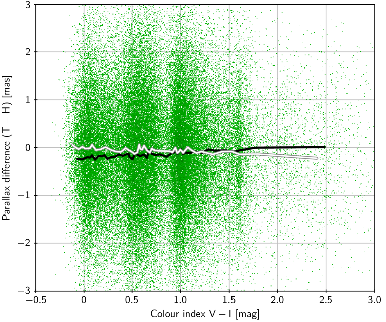
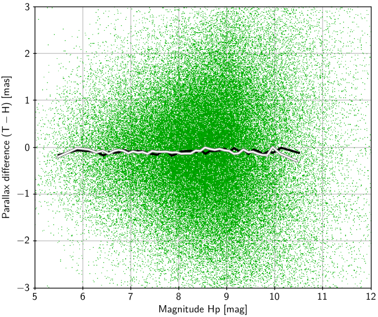
Tycho-2 proper motions

The proper motions in the Tycho-2 catalogue (Høg et al. 2000b) were derived by combining the positions obtained from the Hipparcos star mappers, here called Tycho-2 positions, with positions from earlier transit circle and photographic programs (Høg et al. 2000a), including in particular the Astrographic Catalogue at a mean epoch around 1907 (Urban et al. 1998). Although a big effort was made to put the old positions on the Hipparcos reference frame, systematic errors remain which are then reflected in the Tycho-2 proper motions. For this reason, only the Tycho-2 positions (at the effective epoch of observation around 1991–92) have been used as prior in TGAS, but not the Tycho-2 proper motions.

A comparison of TGAS proper motions with Tycho-2 proper motions will therefore mainly show the errors in the century-old positional catalogues, and is therefore of limited value as a validation of TGAS. Nevertheless, a comparison has been made after rotating the Tycho-2 proper motions to the Gaia DR1 reference frame, using Eq. (8). The global statistics for the proper motion differences (TGAS minus Tycho-2) are $\text{med}(\Delta\mu_{\alpha*})=+0.07$ mas yr^-1, $\text{med}(\Delta\mu_{\delta})=+0.20$ mas yr^-1, $\text{RSE}(\Delta\mu_{\alpha*})=3.6$ mas yr^-1, $\text{RSE}(\Delta\mu_{\delta})=3.3$ mas yr^-1. Maps of median differences are shown in Fig. 21. The maps show significant systematic errors, mainly in zones of constant declination. The alignment of these features with the equatorial coordinate system very clearly points to the old ground-based positions as the main source of systematics.

Figure 21: Differences in proper motion between the primary (TGAS) solution and the Tycho-2 catalogue for 1 997 003 sources: (a) differences in $\mu_{\alpha*}$; (b) differences in $\mu_{\delta}$; and (c) total differences $(\Delta\mu_{\alpha}^{2}+\Delta\mu_{\delta})^{1/2}$. Differences are taken in the sense TGAS minus Tycho-2, after rotation of the latter to the Gaia DR1 reference frame. Median differences are shown in cells of about 0.84 deg². Some empty cells are shown in white. The maps use an Aitoff projection in equatorial (ICRS) coordinates, with origin $\alpha=\delta=0$ at the centre and $\alpha$ increasing from right to left.

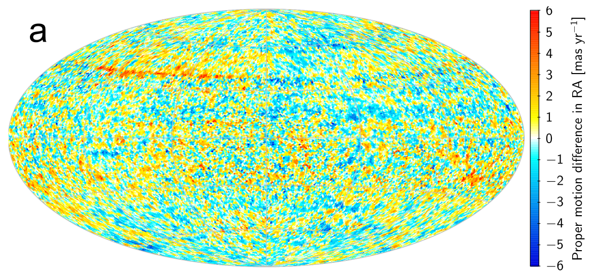
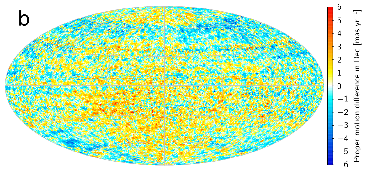
C.2 Quasars

Quasar positions

The auxiliary quasar solution (Sect. 4.2) gave precise positions and parallaxes for more than $10^{5}$ extragalactic sources, including 2191 that were matched to ICRF2 sources with accurate VLBI positions. The defining subset of ICRF2 was used to align the positional reference frame of Gaia DR1 with ICRF2 at epoch J2015.0 as described in Sect. 4.3. Figure 22 shows the optical offsets for both defining and non-defining sources after the alignment. Lumping $\Delta\alpha*$ and $\Delta\delta$ together, the RSE coordinate difference is 0.70 mas for the 262 matched defining sources, and 1.82 mas for the 1929 non-defining sources. Figure 23 shows the distribution of the normalised position differences, $\Delta\alpha{*}/\sigma_{\Delta\alpha*}$, etc., where $\sigma_{\Delta\alpha*}$ is the quadratically combined standard uncertainties in TGAS (auxiliary quasar solution), using the inflated uncertainties, and ICRF2. The RSE of the normalised position differences is 1.08 for the defining sources and 1.02 for the non-defining. The overall agreement is remarkably good, especially considering that no allowance has been made in the error budget for possible radio-optical offsets.

Quasar parallaxes

The true parallaxes of quasars are negligibly small in the present context. The measured values therefore give an immediate impression of the dispersion of parallax errors and possible biases, although a detailed interpretation will be complicated by factors that are peculiar to these objects (optical structure, spectral energy distribution, faintness, sky distribution, etc.). The distribution of measured parallaxes for quasars in the primary solution is given in Figure 24, where separate curves are shown for the northern (88 641 sources) and for the southern ecliptic hemisphere (32 713 sources). The statistics are:

$$\text{med}(\varpi)=\begin{cases}-0.073\pm 0.002\leavevmode\nobreak\ \text{mas}&\text{for $\beta>0$}\,,\\ +0.074\pm 0.005\leavevmode\nobreak\ \text{mas}&\text{for $\beta<0$}\,.\end{cases}$$ (34)

The RSE is 0.85 mas (north) and 1.11 mas (south). The north-south asymmetry in Eq. (34) is stronger than was found in the comparison with Hipparcos data, Eq. (33). However, great caution should be exercised when interpreting the quasar results in view of the many complications mentioned above. Especially the patchy sky coverage of the GIQC is problematic, since local deviations could have a big impact on the global statistics.

A further breakdown of the quasar parallaxes according to colour is then highly interesting. Most of the quasars in GIQC have multicolour photometry from the Sloan Digital Sky Survey (SDSS; York et al. 2000). Figure 25 shows the results of an analysis of nearly 95 000 sources with SDSS colours $g^{\prime}-i^{\prime}$ (Smith et al. 2002). The trends are the same as in Fig. 19, comparing with the Hipparcos parallaxes: a positive trend with increasing colour index for the northern hemisphere, and a negative trend for the southern hemisphere.

Figure 22: Positional offsets of the optical sources matched to the VLBI positions of ICRF2 sources. The blue circles are defining sources in ICRF2, the grey crosses non-defining sources. 2035 sources are inside the displayed area, 156 are outside.

Figure 23: Probability density plots (see footnote 15) of normalised position differences for ICRF2 sources. The solid blue curve is for 262 defining sources, the dashed grey for 1929 non-defining sources. $\Delta\alpha{*}/\sigma_{\Delta\alpha*}$ and $\Delta\delta/\sigma_{\Delta\delta}$ are considered together, as their distributions are not markedly different.

Figure 24: Probability density plots (see footnote 15) of the measured parallaxes of quasars, as obtained in the auxiliary quasar solution. Blue solid curve is for 88 641 sources at northern ecliptic latitudes ($\beta>0$), the red dashed curve for 32 713 sources at southern ecliptic latitudes ($\beta<0$).

Figure 25: Measured parallaxes for 94 795 quasars plotted against SDSS colour index $g^{\prime}-i^{\prime}$. The black line is for northern ($\beta>0$), the grey-white line for southern ecliptic latitudes ($\beta<0$). The lines connect median values calculated in 50 bins subdividing the data according to $g^{\prime}-i^{\prime}$. Each bin contains about 1600 data points for the northern and 300 for the southern latitudes.

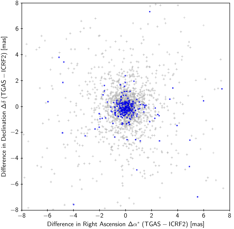
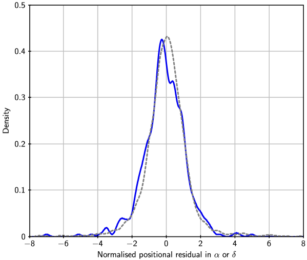
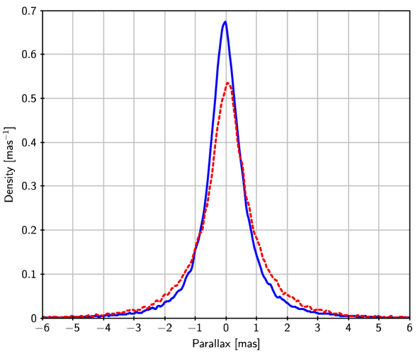
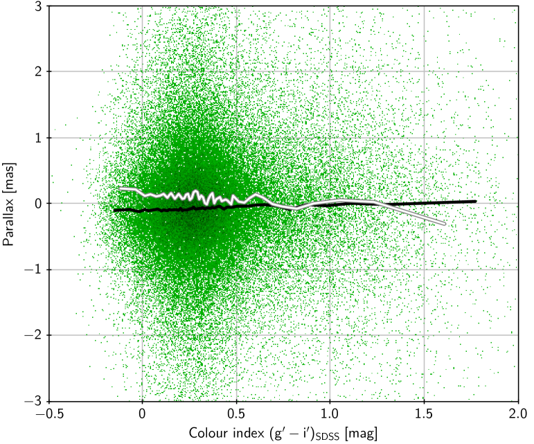
C.3 Galactic cepheids

For distant cepheids the error in the parallax computed from photometric data and a period–luminosity (PL) relation will be small compared with the parallax uncertainty in the current TGAS data. They could therefore provide an independent check of the zero point of the Gaia parallaxes. From the catalogue by Tammann et al. (2003) we retrieved periods and photometric data (mean magnitude $V$, colour excess $E_{B-V}$) for 169 Galactic fundamental-mode pulsators with TGAS parallaxes satisfying Eq. (11). From the PL relation, their parallaxes were computed as

$$\varpi_{\text{PL}}=(100\leavevmode\nobreak\ \text{mas})\times 10^{0.2(a\log P+b-V+R_{V}E_{B-V})}\,,$$ (35)

with $a=-2.678$, $b=-1.275$, and $R_{V}=3.23$ taken from Fouqué et al. (2007). The analysis of differences $\Delta\varpi=\varpi_{\text{T}}-\varpi_{\text{PL}}$ was restricted to the 141 cepheids with $\varpi_{\text{PL}}<1$ mas in order to limit possible biases due to errors in the adopted PL relation, extinction, etc. (For example, a 0.1 mag systematic error in $b$ or in the total extinction translates to a 5% error in $\varpi_{\text{PL}}$, or $<0.05$ mas if $\varpi_{\text{PL}}<1$ mas.) This gave $\text{med}(\Delta\varpi)=-0.016\pm 0.023$ mas and $\text{RSE}(\Delta\varpi)=0.25$ mas. The normalised differences $\Delta\varpi/\sigma_{\varpi}$ have an RSE of 0.86 and a standard deviation of 0.90. A graphical comparison is given in Fig. 26. The north-south asymmetry is insignificant: $\text{med}(\Delta\varpi_{\text{N}})-\text{med}(\Delta\varpi_{\text{S}})=+0.001\pm 0.046$ mas. Indeed, given the median colour index $V-I\simeq 1.3$ mag of the cepheids, very little asymmetry is expected according to Fig. 19. The small number of objects and their limited spread in $V-I$ do not permit a further breakdown according to colour.

Figure 26: Measured (TGAS) parallaxes of Galactic cepheids plotted against their parallaxes computed from photometric data and the $V$ band period-luminosity relation by Fouqué et al. (2007). Error bars are the $1\sigma$ uncertainties in the TGAS parallaxes. The inclined line is the expected 1:1 relation. Only data for the 141 cepheids with $\varpi_{\text{PL}}<1$ mas are shown.

Table 4: Comparison of the astrometric parameters for radio sources in TGAS with the corresponding VLBI results.

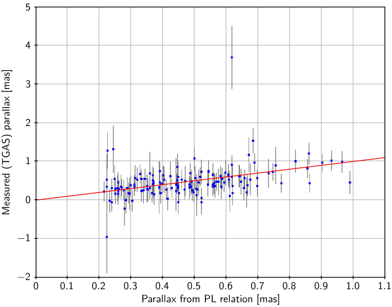
Name	HIP/TYC	$\Delta\alpha*$ [mas]	$\Delta\delta$ [mas]	$\Delta\varpi$ [mas]	$\Delta\mu_{\alpha*}$ [mas yr-1]	$\Delta\mu_{\delta}$ [mas yr-1]	Reference (VLBI)
S Persei	$11093$	$+4.969\pm 8.474$	$-10.626\pm 8.497$	$-0.001\pm 0.720$	$-0.153\pm 0.242$	$-0.225\pm 0.211$	Asaki et al. (2010)
LS I +61 303	$12469$	$-28.882\pm 6.726$	$+22.324\pm 7.611$	$+0.188\pm 0.650$	$-1.322\pm 0.373$	$+1.133\pm 0.383$	Lestrade et al. (1999)
HII 174	1803-0008-1			$-0.024\pm 0.302$	$-0.130\pm 0.918$	$-0.395\pm 0.492$	Melis et al. (2014)
HD 283447	$19762$	$+8.447\pm 0.759$	$-36.971\pm 0.482$	$-0.460\pm 0.495$	$-8.998\pm 0.170$	$+0.011\pm 0.111$	Torres et al. (2012)
T Tau	$20390$	$+231.577\pm 1.280$	$+514.096\pm 0.545$	$+0.291\pm 0.309$	$+7.600\pm 0.169$	$-12.339\pm 0.095$	Loinard et al. (2007)
T Lep	$23636$			$-0.843\pm 0.759$	$-4.395\pm 0.502$	$+1.668\pm 0.791$	Nakagawa et al. (2014)
3C273	$60936$	$+0.912\pm 1.474$	$+0.819\pm 1.961$	$-0.140\pm 0.377$	$-0.384\pm 0.443$	$+0.111\pm 0.288$	Ma et al. (2009)
$\sigma^{2}$ CrB	$79607$	$-12.772\pm 1.142$	$-5.524\pm 1.491$	$+0.104\pm 0.913$	$-0.471\pm 0.065$	$-0.009\pm 0.086$	Lestrade et al. (1999)
Cyg X-1	$98298$	$-0.378\pm 0.444$	$-0.648\pm 0.732$	$-0.310\pm 0.250$	$+0.015\pm 0.086$	$+0.034\pm 0.139$	Reid et al. (2011)
HD 199178	$103144$	$-4.246\pm 8.859$	$+6.620\pm 9.330$	$+0.358\pm 0.474$	$-0.170\pm 0.409$	$+0.349\pm 0.431$	Lestrade et al. (1999)
AR Lac	$109303$	$-4.324\pm 2.945$	$-0.975\pm 4.398$	$-0.332\pm 0.510$	$-0.220\pm 0.127$	$-0.082\pm 0.191$	Lestrade et al. (1999)
IM Peg	$112997$	$+0.503\pm 1.029$	$-0.014\pm 1.046$	$-0.039\pm 0.372$	$+0.001\pm 0.093$	$-0.110\pm 0.096$	Bartel et al. (2015)
PZ Cas	$117078$	$-29.855\pm 3.349$	$-9.348\pm 4.012$	$+0.438\pm 0.558$	$-0.275\pm 0.205$	$-0.236\pm 0.303$	Kusuno et al. (2013)

C.4 Stars observed by VLBI

TGAS results for a small number of sources observed by VLBI are summarised in Table 4. The table includes 12 Galactic sources and one quasar (3C273) for which the quality criteria in Eq. (11) were satisfied. The VLBI data were propagated from the original epoch of the published data to J2015.0, using rigorous formulae for uniform space motion (Butkevich & Lindegren 2014). Radial velocities needed for the propagation were taken from the SIMBAD database (Wenger et al. 2000). The table gives differences in the astrometric parameters computed in the sense TGAS value minus propagated VLBI value. The quoted uncertainties ($\pm 1\sigma)$ are the quadratically combined uncertainties from TGAS and VLBI.

The parallax differences are less than two standard deviations in all cases, and less than one standard deviation for 11 out of the 13 sources. The weighted mean difference for all 13 sources is $\Delta\varpi=-0.060\pm 0.116$ mas.

In position or proper motion there are significant differences (exceeding two standard deviations) for 6 out of the 13 sources. At least four of the objects, namely the young stellar systems T Tau and HD 283447 (V773 Tau), and the RS CVn binary $\sigma^{2}$ CrB, are known to have distant tertiary components causing non-linear proper motions of the inner binaries that contain the radio source (Duchêne et al. 2006, Torres et al. 2012, Lestrade et al. 1999, Peterson et al. 2011). This orbital motion can likely explain the discrepant proper motions for these objects and the large differences between their TGAS positions and the linearly extrapolated VLBI positions. A similar explanation may exist for the X-ray binary LS I +61 303. For the Mira star T Lep and the red supergiant PZ Cas, VLBI observations show multiple maser spots at separations up to $\sim$100 mas and internal kinematics between the spots of a few mas yr^-1 (Nakagawa et al. 2014, Kusuno et al. 2013). These features could explain the position and proper motion differences seen in Table 4 for these two objects.

Appendix D Residual statistics

In this appendix we quantify the overall scatter of the AL residuals of the primary astrometric solution, and discuss some specific contributions to the scatter, i.e. chromaticity, high-frequency attitude noise, and micro-clanks.

D.1 Overall scatter

Figure 27: Solid red curve: the probability density (see footnote 15) of the AL residuals for individual CCD observations in the primary solution. Only good observations (see footnote 8) in a representative five-day interval are included. Dashed blue curve: the normal probability density function with standard deviation 0.667 mas, equal to the RSE of the residuals.

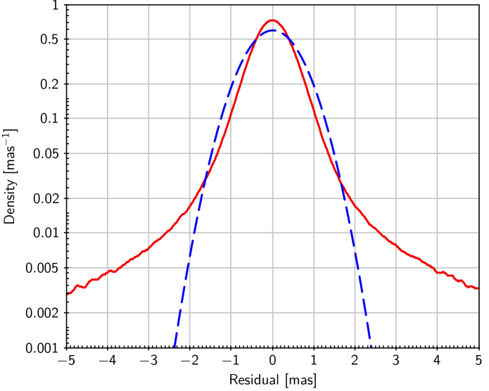
Figure 27 shows the overall distribution of AL residuals in the primary (TGAS) solution. The width, as measured by the RSE, is 0.667 mas. The distribution has a Gaussian-like core with very broad wings. Although only the residuals of good observations (see footnote 8) were used to construct the diagram, some large residuals are included because they have a large excess source noise or excess attitude noise. This explains the presence of the broad wings in Fig. 27.

Figure 28: Along-scan residuals for individual CCD observations in the primary solution as function of colour index $V-I$. Only good observations of Hipparcos stars, made at one particular CCD, are included (row 1 of AF1 in the following field of view; see Fig. 1). Colour indices are taken from the Hipparcos catalogue.

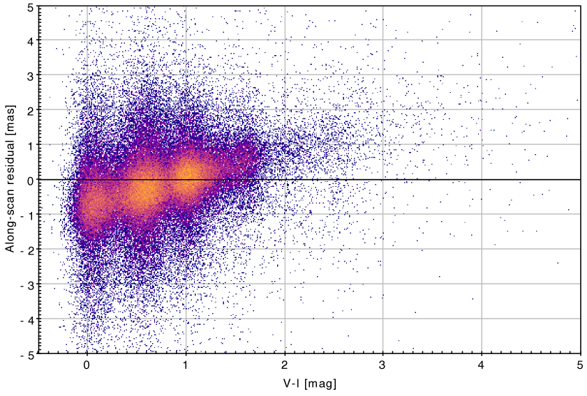
D.2 Chromaticity

Although the AF of the Gaia telescope does not use any refractive optics, the precise location of the centroid of an unresolved stellar image depends on the spectral energy distribution of the star. This phenomenon, known as chromaticity, is the result of a complex interaction of the wavelength-dependent diffraction with asymmetric optical aberrations, pixel geometry, and the centroiding algorithm. Pre-launch simulations, assuming realistic wavefront errors, predicted differential shifts of several mas for a typical range of stellar spectral classes (Busonero et al. 2006). To a first approximation the shift is predicted to be a linear function of the effective wavenumber $\nu_{\text{eff}}$ (Fabricius et al. 2016), which in turn mainly depends on the overall spectral energy distribution in the optical, as given e.g. by the $V-I$ colour index. The chromaticity $\chi$, measured by the shift in mas per magnitude of $V-I$, is expected to vary across the field of view, and to be different in the preceding and following fields. To the extent that the optical aberrations vary with time, chromaticity will also be a function of time.

A plot of the AL astrometric residuals versus $V-I$ for the Hipparcos subset (using colour indices from the Hipparcos catalogue) reveals significant chromaticity, as exemplified by Fig. 28. Different CCD/field-of-view combinations give slopes roughly in the range $\left|\,\chi\,\right|\lesssim 1$ mas mag^-1. Some fraction of this shift propagates into the astrometric parameters of a source, depending on the number and geometry of the scans across the source. Simulated TGAS runs show that the resulting shift in parallax is of the order of $\pm 0.2$ mas mag^-1, with a strong dependence on position. This effect is more directly studied by introducing colour-dependent calibration terms, as described in Appendix E.1.

Figure 29: Cross-correlation of the astrometric residuals in the preceding and following fields of view.

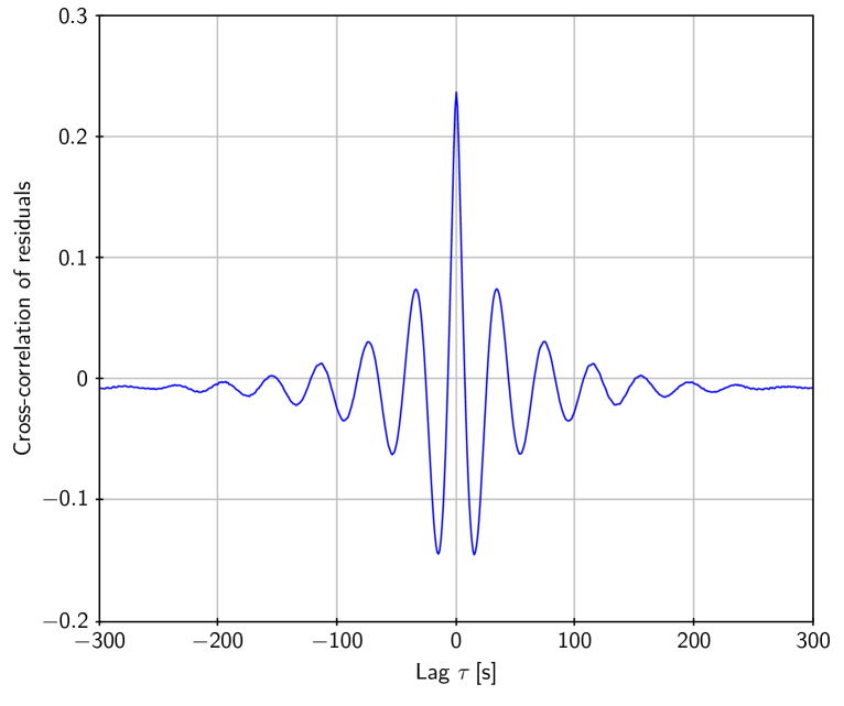
D.3 Correlations

The top panel of Fig. 34 shows, for a short stretch of observations, the AL residuals in the baseline primary solution. The wiggles, having an amplitude of $\simeq 0.5$ mas, are representative for the overall quality of the attitude fit. This indicates that much of the residual variance seen in Fig. 27 comes from AL attitude irregularities that are too rapid to be modelled by the attitude spline with a 30 s knot interval (Appendix E.4). The resulting modelling errors introduce temporal correlations in the observations on timescales up to several minutes, which in turn propagate into spatial correlations among the astrometric parameters.

An analogous situation for the Hipparcos data was analysed by van Leeuwen (2007b), who demonstrated how a careful modelling of the attitude can reduce not only the total size of the modelling errors but also the temporal (and hence spatial) correlations by a large factor. For Gaia, this will be remedied in future data releases. In the meantime, it is important to characterise the correlations that exist in Gaia DR1.

Figure 29 is a plot of the cross-correlation coefficient between the AL residuals in the two fields of view, calculated as

$$\rho_{pf}(\tau)=\frac{\overline{p_{i}f_{j}}}{\sigma_{p}\sigma_{f}}\,,$$ (36)

where $p_{i}$ and $f_{j}$ are the residuals of observations in the preceding and following field of view, respectively, and the average is taken over all residual pairs for which the time difference $t_{i}-t_{j}$ is $\tau$ (to the nearest second). The normalisation factor is $\sigma_{p}\sigma_{f}=0.38$ mas², from which the cross-covariance can be recovered.

The cross-correlation function exhibits the characteristic pattern expected from modelling errors in the attitude spline. Given that the knot separation is 30 s, it may seem surprising that the zero-crossings have a typical separation of only about 20 s; however, this is expected for an attitude spline fit using a small value of the regularisation parameter $\lambda$ (Sect. 3.5; see Holl et al. 2012). The height of the central peak suggests that at least a quarter of the total residual variance comes from attitude modelling errors. The actual fraction may be higher (see below).

For lags of several minutes, the cross-correlation function in Fig. 29 settles at a slightly negative value, corresponding to a cross-covariance of $-2600\leavevmode\nobreak\ \mu$as². This is caused by basic-angle variations that have not been corrected based on the BAM data, nor accounted for in the calibration. Since the AL attitude is defined by the mean pointing of the two viewing directions, residuals caused by basic-angle variations are anti-correlated between the fields. The rms amplitude of these (as yet) uncalibrated basic-angle variations is $(2\times 2600)^{1/2}\simeq 72\leavevmode\nobreak\ \mu$as. (For much bigger lags of several hours the cross-covariance gradually goes to zero, except around values related to the spin period and basic angle.)

The temporal correlations shown in Fig. 29 are significant for delays up to $\sim$2 min, corresponding to $2^{\circ}$ on the sky. Thus, spatial correlations in the astrometric parameters can be expected for stars that are separated by angles up to a few degrees. The extent to which the temporal correlations propagate into spatial correlations depends in a complex way on the geometry of the scans and how much overlap there is between the scans of the different stars. A rough indication is given by the “coincidence fraction” introduced by van Leeuwen (1999, 2007b) in the context of Hipparcos data. For Hipparcos observations the coincidence fraction drops rapidly from close to 1 at very small separations to 0.5 at separations of ${\sim}1^{\circ}$, and then more slowly. The same should be the case for Gaia observations, as the scanning laws and field sizes of the two missions are rather similar. Thus we conclude that the spatial correlations in the Gaia DR1 astrometry, e.g. for parallaxes in a stellar cluster, may be significant (perhaps $\sim$0.25) at separations up to ${\sim}1^{\circ}$, but much smaller on longer scales. In this context it should be remembered that Fig. 29, being derived from the residuals of the solution, inevitably underestimates the cross-correlation of the actual attitude modelling errors, which to some extent are absorbed by the source parameters. Other modelling errors may create astrometric errors that are correlated over much longer angular scales (Appendix E).

Figure 30: Top panels: examples of micro-clanks in the AL TGAS residuals during a time interval of 500 s (left) and a subinterval of 50 s (right). The vertical lines show the times of the micro-clanks as estimated from rate data (red/blue for positive/negative jumps). The attitude knot interval is 30 s, which sets the typical period of the wiggles seen between the micro-clanks. In the top right panel, filled blue dots are ungated observations and open red circles are gated observations. The shorter integration time of the gated observations gives a steeper slope of the residuals around the micro-clanks, as can be seen, for example, by comparing the open red circles and filled blue dots around the jump at 303 s in the top right panel. Bottom panels: AL inertial angular rates estimated from successive ungated CCD observations of a much larger number of faint ($\sim$15 mag) stars. Individual rate estimates are shown as blue dots. The thick magenta curve shows the median rate estimate in each bin of 0.045 s duration. The black curve is a 5-point running triangular mean of the medians, added to better show the rate variations. The vertical lines at the bottom of the diagram show the estimated times of the micro-clanks detected by means of a simple matched filter.

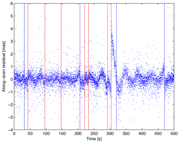
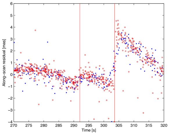
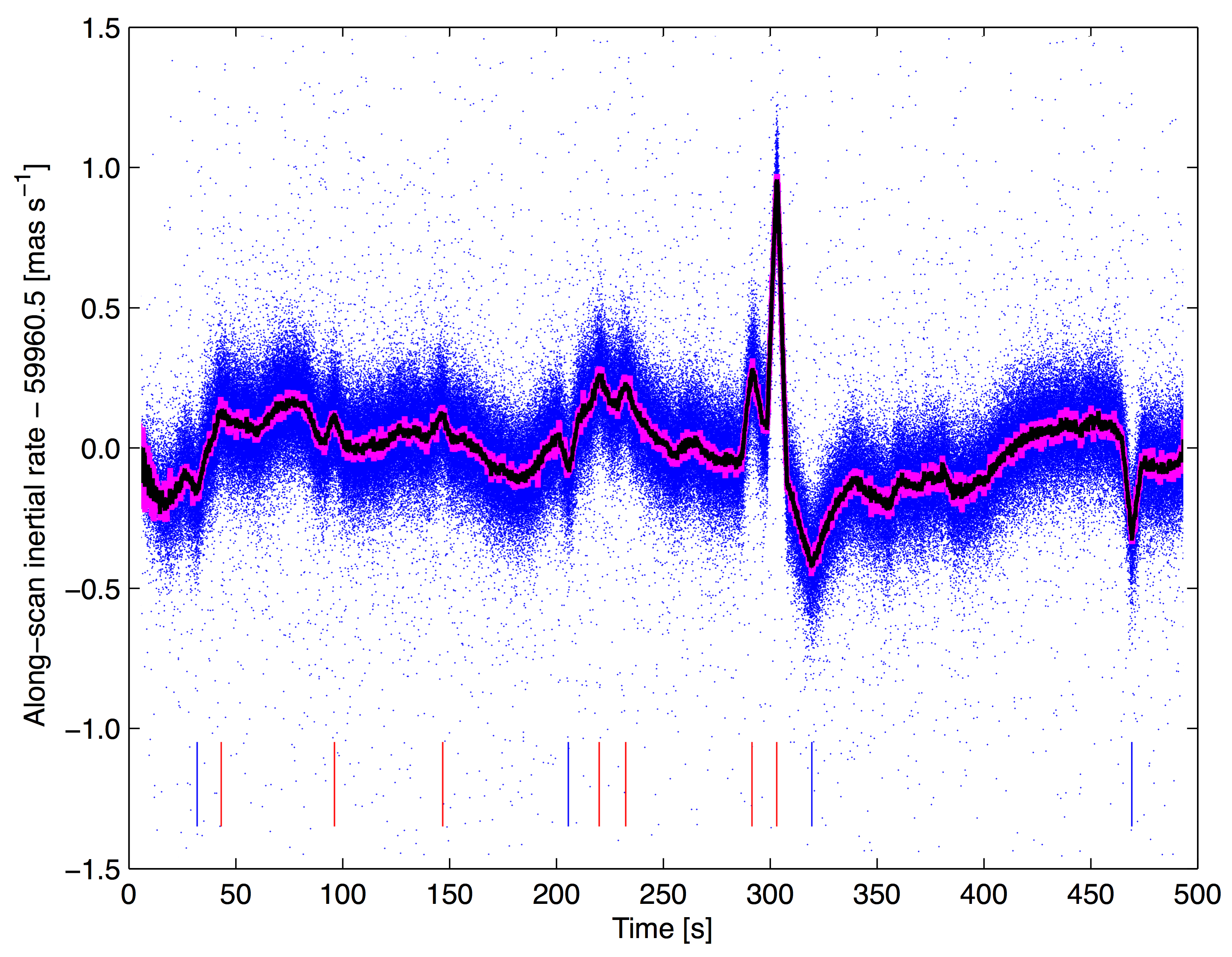
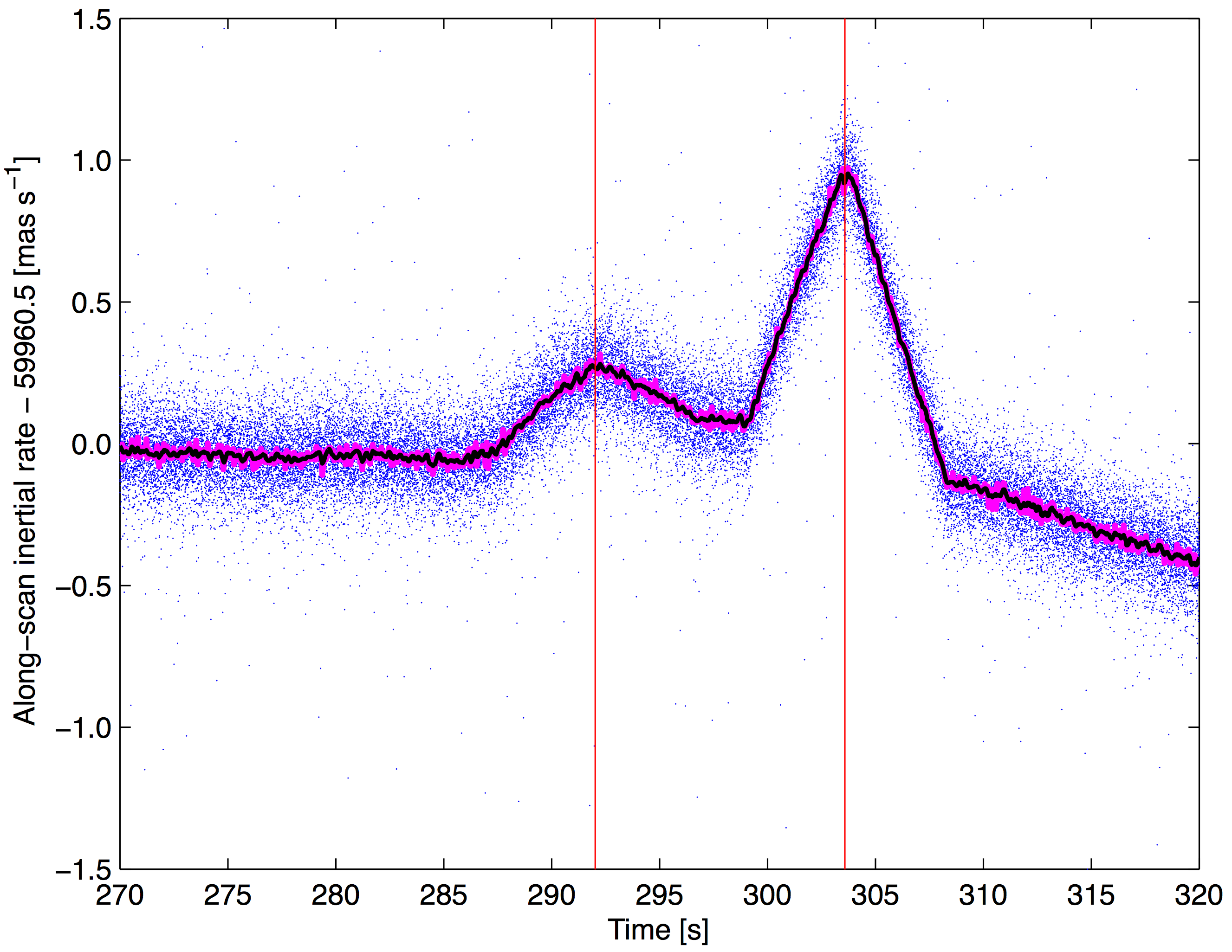
D.4 Micro-clanks

Soon after Gaia’s launch, small rapid rotation rate changes of the spacecraft were discovered at a frequency of about one every few minutes, with amplitudes up to a few mas s^-1. These were initially interpreted as micrometeoroid hits. However, based on more and better data, the observed rotation rate excursions were later identified to be almost all caused by sudden small structural changes within the spacecraft (Gaia collaboration, Prusti, et al. 2016). They are here referred to as micro-clanks. Their physical origins are still unclear. Micro-clanks are seen both in the AL and AC directions, and they often repeat quasi-periodically with the spin period of the satellite. In the AL direction, the vast majority of them affect both fields of view equally and simultaneously, with no discernible effect in the BAM data, which suggests an origin outside of the optical instrument. For a small fraction of them, however, the times coincide with jumps in the BAM fringe-position data, which may be different for the two fields of view or only seen in one of the fields. These micro-clanks apparently originate within the mechanical structure of the optics.

Whatever the origin may be, the effect of a micro-clank is a quasi-instantaneous discontinuity (on timescales $\ll 1$ s) in the physical attitude angle, while the physical attitude rate is practically the same on either side of the discontinuity. However, since the physical attitude angle is not directly observable, but only a moving average over the CCD integration time (the so-called effective attitude; Risquez et al. 2013), the effect as seen in the astrometric residuals is not instantaneous but linear over the CCD integration time, which is 4.42 s for ungated observations, and shorter for gated observations. The left panels of Fig. 30 show the AL TGAS residuals in a 500 s time interval, with clear evidence of several micro-clanks. The vertical lines show the times of all the micro-clanks detected in rate data (see below) for this interval. In the zoomed-in plot, the effect of the CCD integration time is clearly seen.

The micro-clanks in Gaia data were first seen in AL rate estimates, computed from the precise time difference of successive CCD observations, separated by approximately 4.85 s, of the same star. Rate estimates (both along and across scan) are very much easier to compute than the astrometric residuals, as they are purely differential and hence independent of source parameters and less sensitive to calibration errors; they can also easily be computed for many more stars. The bottom panels in Fig. 30 show early AL rate estimates for the same time intervals as in the top panels. These were computed from ungated observations of much fainter stars than in TGAS. The CCD integration time of 4.42 s and the time difference of 4.85 s between successive observations result in apparent rate excursions around the time of each micro-clank, with a completely predictable and very characteristic trapezoidal (almost triangular) profile. The time and amplitude of the micro-clank can be estimated very precisely from such rate data, essentially by using a matched filter. In this 500 s interval, no less than 11 micro-clanks were thus detected, as indicated by the vertical lines. The astrometric residuals clearly confirm at least ten of them. In a longer time interval of 72 min, some 120 micro-clanks were detected with amplitudes corresponding to AL attitude discontinuities in the range from 0.3 mas to 4.3 mas. The largest micro-clank in this interval is the one seen in Fig. 30 at 303 s. It appears that they rarely get much bigger than this. In all the time intervals that have so far been investigated in detail, their frequency was similar to the numbers given above.

Based on the limited statistics reported above, the effective attitude for ungated observations is directly disturbed by micro-clanks for at least $\sim$10% of the time. If left uncorrected, the micro-clanks are therefore a major source of attitude noise. In the present TGAS results they enter as statistical modelling noise. For future astrometric solutions they must be largely eliminated. The originally foreseen strategy to handle clanks was to insert multiple knots in the attitude spline at the relevant times (see Sect. 5.2.5 and Appendix D.4 of the AGIS paper). However, with the observed high frequency of micro-clanks, such a procedure would weaken the attitude estimation considerably. It is now clear that a far better strategy is to apply gate-dependent corrections based on the times and amplitudes of micro-clanks, detected and quantified in the rate data. This will be implemented in the AGIS pre-processor for future Gaia data releases.

Appendix E Special validation solutions

In this appendix we briefly describe some of the special TGAS runs that were computed in order to test the sensitivity of the baseline TGAS run to various modelling assumptions. Since a primary concern is the existence of systematic errors in the parallaxes, we focus on characterising how the parallaxes change with respect to the baseline solution. Parallax differences are always computed in the sense baseline solution minus special validation solution.

E.1 Including colour terms in the calibration

As shown in Appendix D.2, the AL residuals for a particular CCD/field of view combination have an approximately linear dependence on the colour index $V-I$ owing to the chromaticity of the instrument. This effect can therefore largely be eliminated by including colour-dependent terms in the geometric calibration model (Appendix A.1).

Figure 31: Differences in parallax between the baseline primary solution and a special validation solution with colour terms in the calibration model. (a) Blue sources (colour index $C\leq 0.75$). (b) All TGAS sources. (c) Red sources ($C>0.75$). Median differences are shown in cells of about 3.36 deg². The maps use an Aitoff projection in equatorial (ICRS) coordinates, with origin $\alpha=\delta=0$ at the centre and $\alpha$ increasing from right to left.

Figure 32: Differences in parallax between the baseline primary solution and a special validation solution where the data are split into early and late observations (within the AF). (a) Baseline minus late. (b) Baseline minus early. (c) Late minus early. Median differences are shown in cells of about 3.36 deg². The maps use an Aitoff projection in equatorial (ICRS) coordinates, with origin $\alpha=\delta=0$ at the centre and $\alpha$ increasing from right to left.

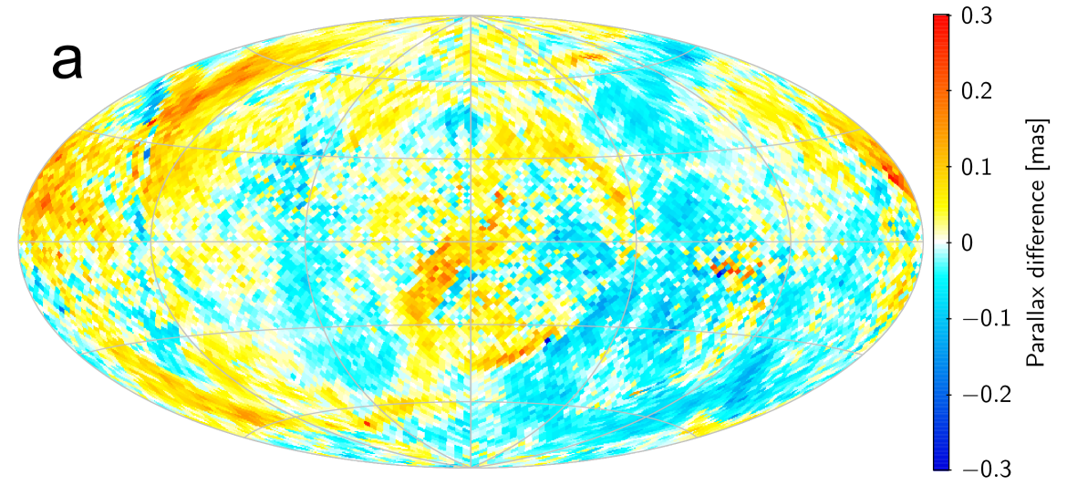
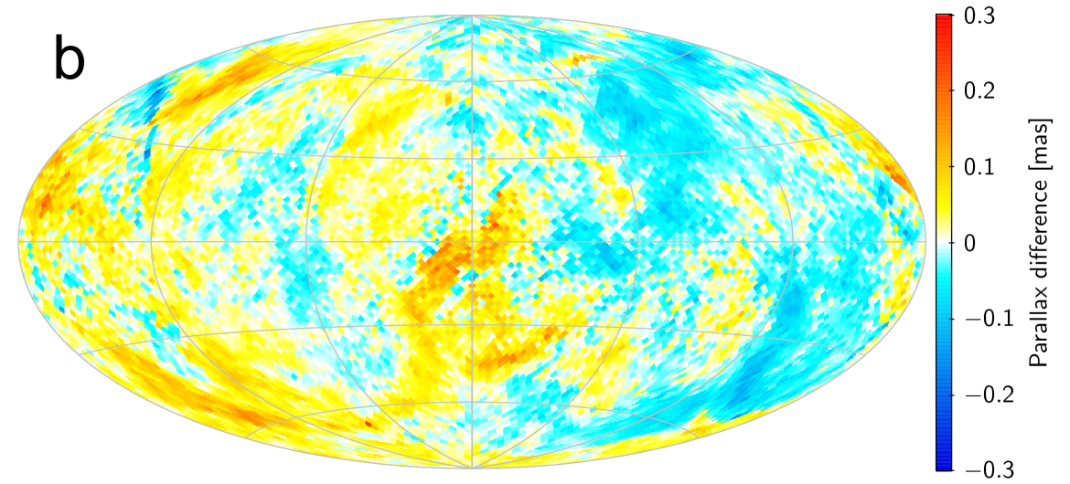
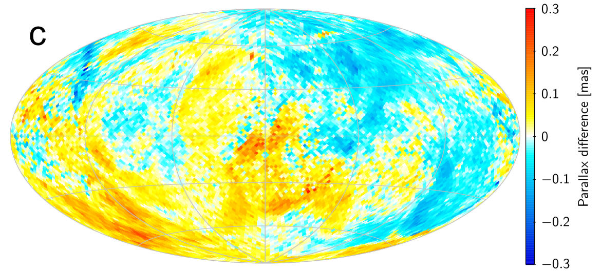
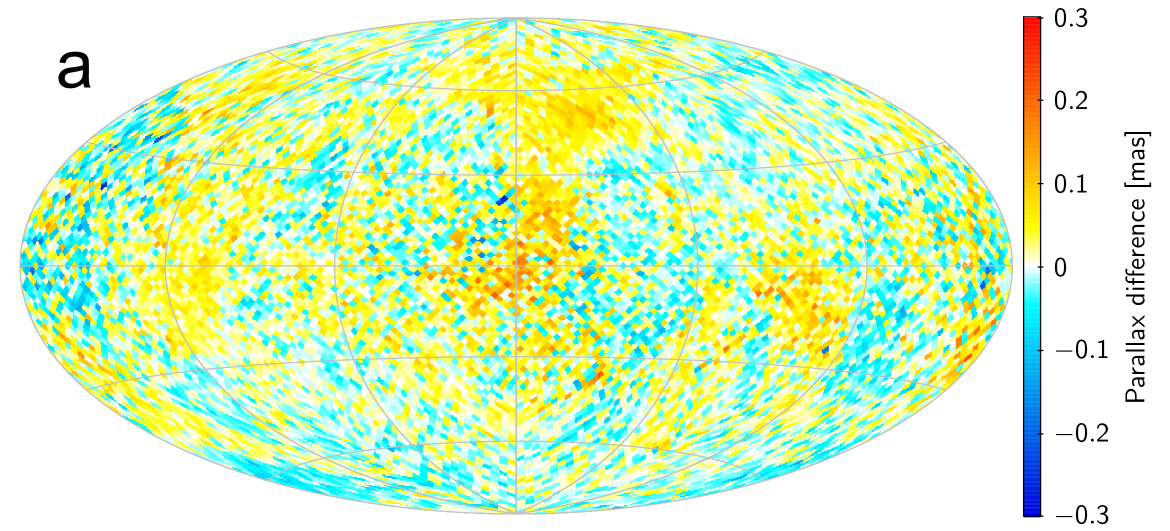
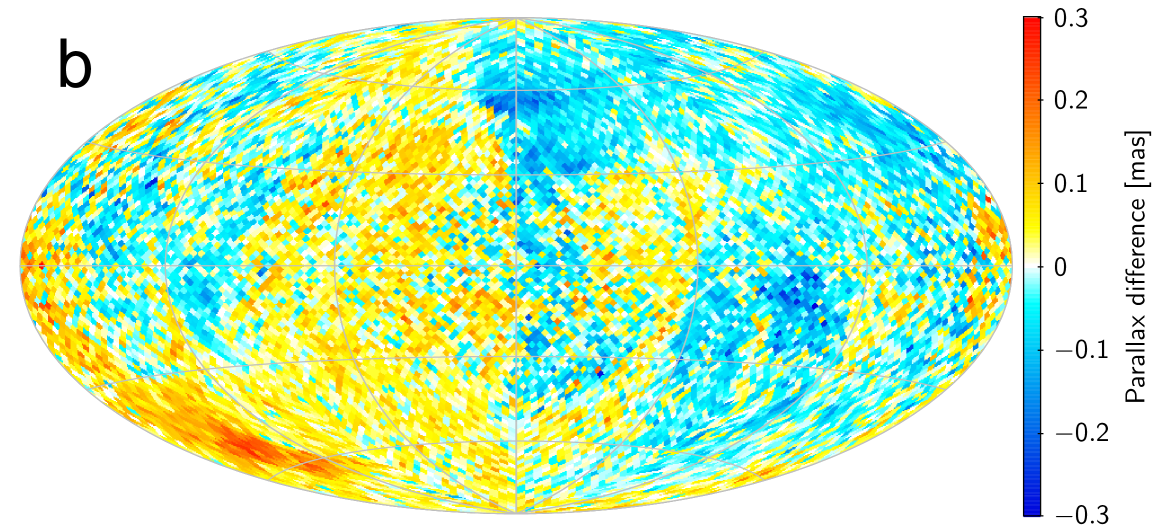
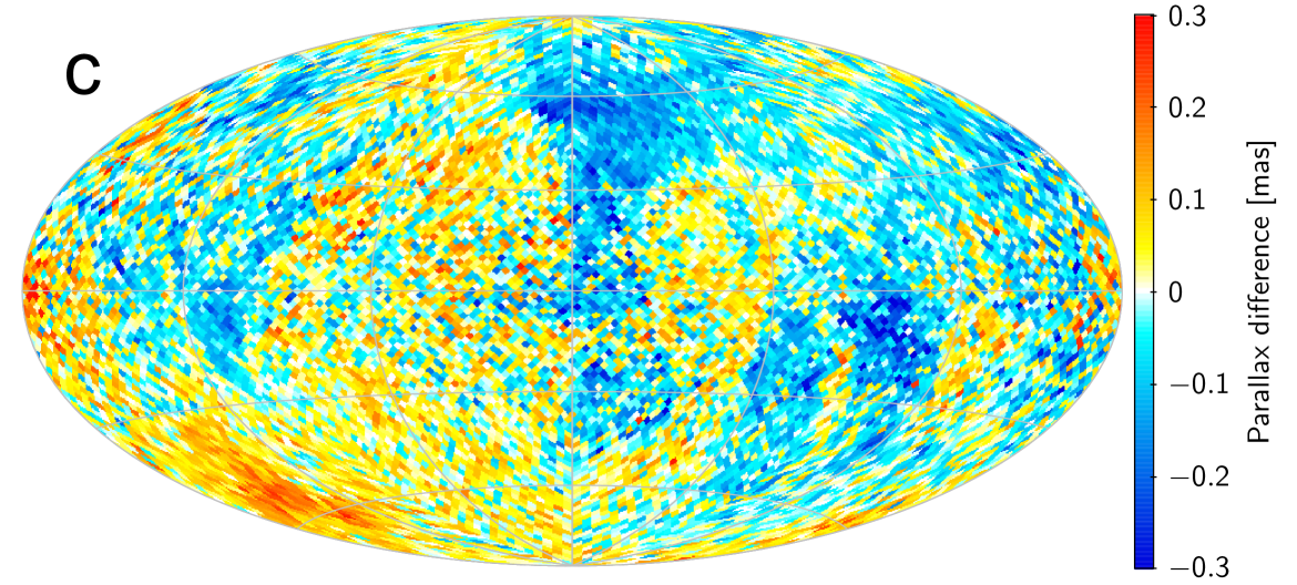
While Gaia will eventually provide excellent colour information on all observed sources through its blue and red photometers (BP and RP in Fig. 1; van Leeuwen et al. 2016), this information was not available at the time when the TGAS baseline and validation solutions were computed. For the present test it was therefore necessary to compile colour information from available external sources. For most Hipparcos stars, $V-I$ from the Hipparcos catalogue could be used. For many Tycho-2 stars, provisional (uncalibrated) BP and RP magnitudes were available, while for others 2MASS photometry ($J{-}K_{s}$) or Tycho colours ($B_{T}{-}V_{T}$) had to be used. In all cases, linear transformations were applied to put the resulting colour index (hereafter denoted $C$) on approximately the same scale as $V-I$. While the resulting colours are thus of extremely inhomogeneous quality, and the applied transformations often quite uncertain, this $C$ is still useful for a statistical evaluation of the chromaticity. The median $C$ is close to 0.75 mag, roughly corresponding to a solar-type star.

For this validation solution, the geometric AL calibration model in Eq. (13) was augmented with terms

$$\eta_{fngw}(\mu,\,t,\,C)=\cdots+\chi_{fnwj}(C-0.75)\,,$$ (37)

where $\chi_{fnwj}$ are chromaticity parameters (Appendix D.2) depending on the field of view ($f$), CCD ($n$), window class ($w$), and time interval ($j$). The time resolution is the same as for the large-scale AL calibration, i.e. typically 3 days. (The coefficient of the chromaticity is offset by 0.75 mag to reduce correlations among the calibration parameters. The choice of offset is in principle arbitrary and does not affect the astrometric part of the solution, but simply means that the attitude and non-chromatic calibration parameters refer to sources of colour index 0.75.)

Figure 31 shows median parallax differences (baseline minus solution with colour terms) for three source selections: “blue” (1.039 million sources with colour index $C\leq 0.75$; $\text{med}(C)=0.58$), all (2.087 million sources; $\text{med}(C)=0.75$), and “red” (1.047 million sources with $C>0.75$; $\text{med}(C)=1.13$). Somewhat surprisingly, the blue and red maps are not vastly different, and in particular they are not inverted versions of each other, as could be expected if the parallax dependence on colour, $\text{d}\varpi/\text{d}C$, was simply a function of position. Rather, it appears that the chromaticity creates time-dependent attitude errors in the baseline solution, which then propagate into position dependent astrometric errors that are partly independent of the colour. The median parallax difference is small and practically the same for all three selections ($+0.004$, $+0.004$, $+0.005$ mas, respectively, for blue, all, and red sources). The RSE (0.128, 0.146, and 0.168 mas, respectively) is larger for the red sources, which could simply be because the scatter of $C$ is larger for the red sample ($\text{RSE}(C)=0.33$ mag) than for the blue ($\text{RSE}(C)=0.19$ mag).

In summary, the overall effect of chromaticity on the TGAS parallaxes is of the order of $\pm 0.15$ mas (random), with position and colour dependent systematics of $\pm 0.1$ mas, although the systematics may exceed $\pm 0.2$ mas in some parts ($\sim$1%) of the sky.

E.2 Partitioning the data

During a field of view transit, a source is generally observed on all nine CCD strips of the astrometric field (AF1 through AF9; see Fig. 1). Since the sky mapper data are not used in TGAS, and all nine AF observations provide AC measurements for bright (window class 0) sources, it is possible to partition the observations into almost completely independent data sets based on the CCD strip number. Here we describe the results of two validation solutions, one using AF1–AF4 (“early”) data, the other using AF5–AF8 (“late”) data. Because the two solutions use completely different parts of the focal plane, they are differently affected by any unmodelled instrumental effect that varies across the fields of view. For example: the parallax zero point is known to be tightly correlated with the harmonic coefficient $C_{1,0}$ of the basic-angle variations (see Appendix E.3). However, the relevant basic-angle variations are an average over the actually used part of the AF (see Eq. 17), and could therefore be slightly different for the early and late observations. If this is the case, there might be a zero-point shift between the parallaxes in the two solutions.

The early/late partitioning also introduces a time shift of about 19.4 s between the early and late data, which should make the astrometric effects of short-range attitude modelling errors rather different in the two solutions.

The following comparisons are limited to some 2.05 million sources that have formal (uninflated) parallax standard uncertainties $\varsigma_{\varpi}<1$ mas in both the early and late solutions. Figure 32 shows maps of the median parallax differences between the different solutions. The global median and RSE values are given in Table 5.

Table 5: Statistics of parallax differences between the baseline TGAS solution ($\varpi_{\text{T}}$) and the two special validation solutions using only early ($\varpi_{\text{E}}$) and late ($\varpi_{\text{L}}$) observations from each field-of-view transit.

Difference	median	RSE
$\varpi_{\text{T}}-\varpi_{\text{L}}$	$+0.0114\pm 0.0002$ mas	0.235 mas
$\varpi_{\text{T}}-\varpi_{\text{E}}$	$+0.0041\pm 0.0003$ mas	0.290 mas
$\varpi_{\text{L}}-\varpi_{\text{E}}$	$-0.0065\pm 0.0004$ mas	0.463 mas

Although the global parallax zero points of the three solutions differ by less than 0.02 mas, the difference maps in Fig. 32 show systematic, position-dependent errors of $\pm 0.1$ mas or more. There are distinct similarities between these maps and the chromaticity maps in Fig. 31, which suggests that the much larger chromatic effects could mask any possible difference in the effective basic-angle variations between the early and late data. In conclusion these solutions mainly confirm the existence of position-dependent systematics at the level of $\pm 0.1$ to 0.2 mas.

E.3 Solving the basic-angle variations

As described in Sect. 3.7 and Appendix A.2, the baseline primary (TGAS) solution of Gaia DR1 was computed after correcting the observations for the basic-angle variations as estimated from the BAM data. This was done by first fitting the harmonic model in Eqs. (22)–(23) to the BAM data, and then using the fitted model to evaluate the correction as function of time (or heliotropic phase angle $\Omega$). The BAM uses a dedicated CCD located outside of the AF (see Fig. 1). Thus, although the BAM measurements are intrinsically very precise ($<10\leavevmode\nobreak\ \mu$as per measurement), it is possible that they do not correctly describe the basic-angle variations relevant to the observations in the AF. This would be the case, e.g. if the AL scale of the astrometric field (angle between the successive CCD strips) also has a periodic variation with $\Omega$. The correction relevant for a particular observation is a combination of the basic-angle correction $\Delta\Gamma(t)$ and a possible differential variation between the two fields of view, $\Delta\eta(t,\,\eta,\,\zeta)$, the latter being a function of both time and the field angles. From simplistic optomechanical considerations it is reasonable to expect that the differential correction $\Delta\eta(t,\,\eta,\,\zeta)$ is of the order $O(\eta-\eta_{\text{BAM}})\sim 0.01$ times smaller than the actual basic-angle variation. This would not have been a problem if the basic-angle variation itself was of the order of 10 $\mu$as as expected from pre-launch calculations (Gaia collaboration, Prusti, et al. 2016). However, since the variations are now known to be of the order of 1 mas, a possible differential variation over the field of view becomes a point of concern. A related issue concerns the representativeness of the BAM data, given that the laser beams of the BAM interferometer only sample a very small part of the telescope entrance pupil.

In view of these uncertainties, it is clearly desirable to estimate as much as possible of the short term ($\lesssim 24$ hr) basic-angle and differential field of view variations directly from the astrometric data. Detailed simulations indicate that this will eventually be possible, provided that the basic-angle variations are constrained by suitable models, e.g. in the form of a generalisation of Eqs. (22)–(23). One possible exception is the constant part of the $\cos\Omega$ coefficient, corresponding to $C_{1,0}$ in Eq. (23), which is almost completely degenerate with respect to a global error of the parallax zero point (Lindegren et al. 1992, Michalik & Lindegren 2016). Further details will be discussed elsewhere.

Table 6: Fourier coefficients $C_{k,0}$, $S_{k,0}$ from the BAM data and as obtained in a special validation run of the TGAS primary solution.

	BAM	Solution			BAM	Solution
	[$\mu$as]	[$\mu$as]			[$\mu$as]	[$\mu$as]
$C_{1,0}$	$+865.07$	(fixed)		$S_{1,0}$	$+659.83$	$+605.66$
$C_{2,0}$	$-111.76$	$-134.66$		$S_{2,0}$	$-85.26$	$-77.34$
$C_{3,0}$	$-67.84$	$-76.14$		$S_{3,0}$	$-65.91$	$-63.34$
$C_{4,0}$	$+18.26$	$+24.98$		$S_{4,0}$	$+17.79$	$+19.40$
$C_{5,0}$	$+3.20$	$+7.42$		$S_{5,0}$	$-0.20$	$-6.44$
$C_{6,0}$	$+3.51$	$+6.31$		$S_{6,0}$	$+0.68$	$+1.02$
$C_{7,0}$	$+0.03$	$+1.45$		$S_{7,0}$	$+0.34$	$-0.31$
$C_{8,0}$	$-0.62$	$-2.87$		$S_{8,0}$	$-0.59$	$-6.56$

Figure 33: Differences in parallax between the baseline primary solution (where basic-angle variations are corrected based on BAM data) and a special validation solution where the harmonic coefficients $C_{k,0}$, $S_{k,0}$ (except $C_{1,0}$) were instead estimated as global parameters in the solution. Median differences are shown in cells of about 0.84 deg². The map uses an Aitoff projection in equatorial (ICRS) coordinates, with origin $\alpha=\delta=0$ at the centre and $\alpha$ increasing from right to left.

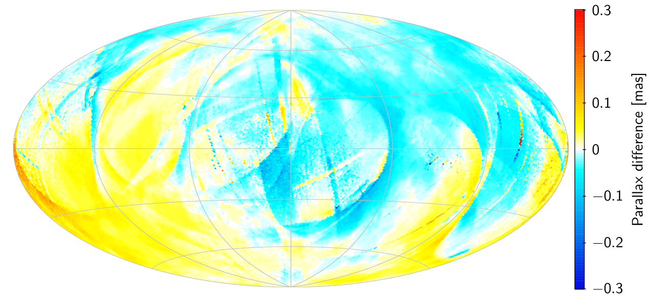
Special algorithms and software packages to recover both basic-angle and differential variations have been developed and tested in AGIS. This software will be used in the astrometric solutions of future data releases to mitigate these effects. The software was however not used for the current baseline solution, for which we instead assume that the BAM provides adequate corrections. Nevertheless, for validation purposes we have made TGAS runs where the harmonic coefficients $C_{k,m}$, $S_{k,m}$ are estimated as global parameters for $k=1\dots 8$ and $m=0,\,1$ (but excluding $C_{1,0}$). The time interval covered by the current data is not long enough to reliably estimate the linear time-dependent coefficients ($m=1$). Results for the time-independent coefficients ($m=0$) are shown in Table 6 along with the corresponding coefficients estimated from the BAM data. In this solution $C_{1,0}$ was fixed at its value according to the BAM. In general the coefficients obtained in the TGAS run are in good agreement with the BAM data; the largest difference (about 0.05 mas) is obtained for $S_{1,0}$. The corresponding parallax differences (baseline solution minus special validation solution), shown in Fig. 33, have a median value of $+0.006$ mas and an RSE of 0.035 mas. The distinct asymmetry in ecliptic latitude, with an amplitude of about 0.05 mas, is related to the particular differences in the values of $C_{k,m}$ and $S_{k,m}$ as given in Table 6 and most importantly to the difference in $S_{1,0}$.

E.4 Changing the attitude model

The attitude model is completely defined by the knot sequence, which for the baseline primary solution uses a regular sequence with a knot interval of 30 s, but with additional knots inserted at certain times to allow discontinuities in the attitude quaternion in connection with data gaps. Changing the knot sequence results in a different solution, which is not necessarily better, but the difference between two such solutions (e.g. in parallax) gives an indication of how critical the attitude modelling is. For a regular knot sequence, the main parameters that can be changed are the time of the first knot and the interval between successive knots. Here we describe briefly the results of validation runs implementing such changes. (The order of the spline is also a configurable parameter in AGIS, but all solutions described in this paper use a fourth-order, or cubic, spline.)

Figure 34: Along-scan residuals of individual CCD observations vs. time for an interval of 500 s. Blue and red dots represent observations in the preceding and following field of view, respectively. Only good observations are shown. The vertical grey lines mark the times of the knots for the attitude spline. Top: residuals from the baseline primary solution. Middle: residuals from the special validation solution with shifted knot sequence. Bottom: residuals from the special validation solution using a shorter knot interval of 15 s.

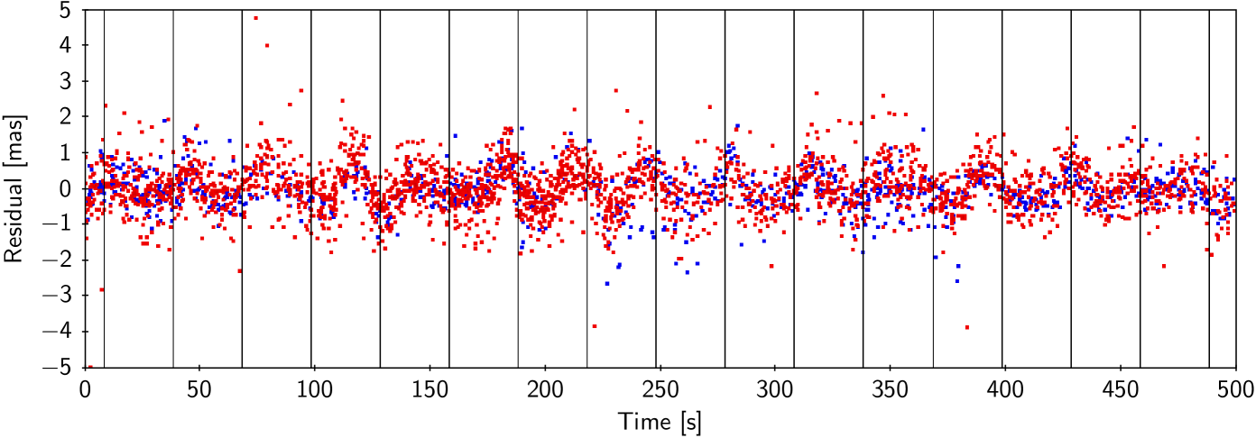
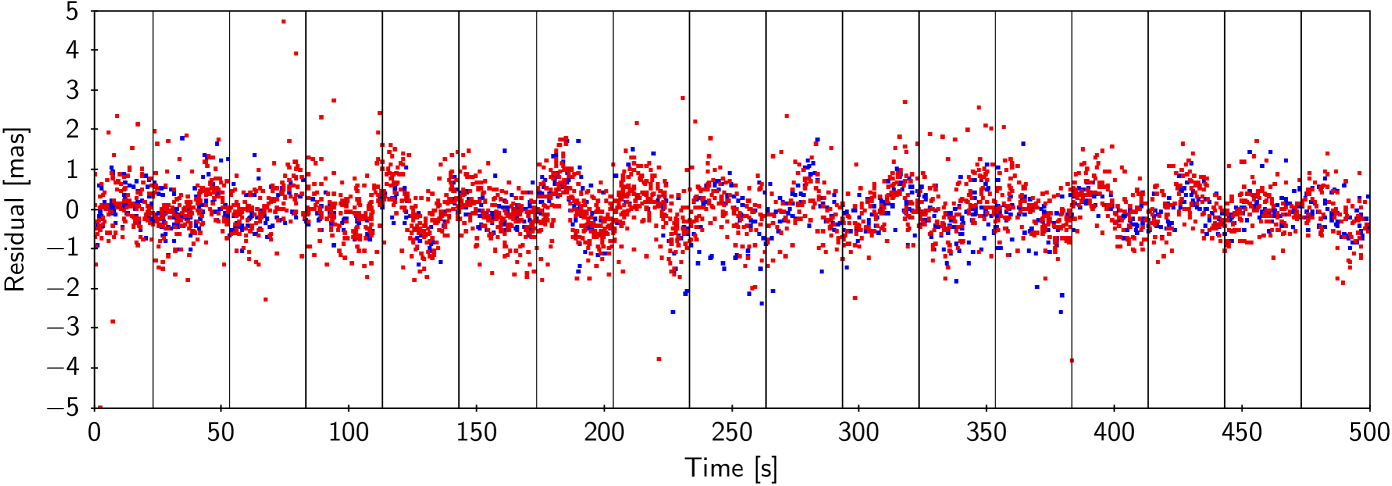
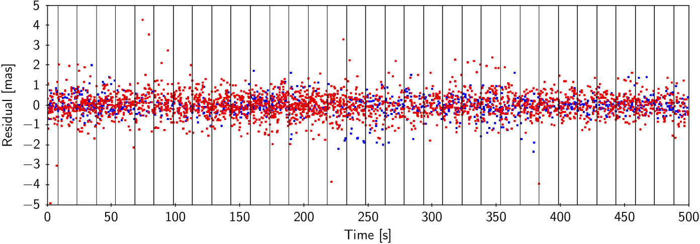
Shifting the knot sequence

A validation solution was computed using the same 30 s knot interval as in the baseline solution, but shifting the knots by 15 s. For most of the time, this has very little effect on the residuals. This can be seen by comparing the top two panels of Fig. 34. Some details are clearly different, but the main features, in particular the quasi-periodic wiggles, are almost identical. This shows that these features represent real high-frequency ($\gtrsim 0.03$ Hz) components of the AL attitude irregularities, with the spline fitting basically acting as a high-pass filter. Significant differences are seen in connection with the larger micrometeoroid hits, but they affect only a small fraction of the time and sources. The global RSE of the parallax difference between the two solutions is 0.024 mas.

Reducing the knot interval

The 30 s knot interval used for the baseline primary solution was chosen because it gives at all times a sufficient number of AL and AC observations per knot interval. Reducing the knot interval to 15 s gives a less stable attitude solution, but the attitude modelling errors are significantly reduced, as shown by the bottom panel of Fig. 34. Compared with the baseline solution, the RSE of the residuals is reduced by about 15%. The global RSE of the parallax difference between the baseline solution and the solution using a 15 s knot interval is 0.069 mas.