Estimating the Distance Between Macro Base Station and Users in Heterogeneous Networks

Lin Zhang∗†, Wenli Zhou, Wanbin Tang, Gang Wu, and Zhi Chen
* NCL, University of Electronic Science and Technology of China, Chengdu, China
{\dagger} Science and Technology on Information Transmission and Dissemination
in Communication Networks Lab., China
This work is supported by Scinece and Technology on Information Transmission and Dissemination in Communication Networks Laboratory.
Abstract

In underlay heterogeneous networks (HetNets), the distance between a macro base station (MBS) and a macro user (MU) is crucial for a small-cell based station (SBS) to control the interference to the MU and achieve the coexistence. To obtain the distance between the MBS and the MU, the SBS needs a backhaul link from the macro system, such that the macro system is able to transmit the information of the distance to the SBS through the backhaul link. However, there may not exist any backhaul link from the macro system to the SBS in practical situations. Thus, it is challenging for the SBS to obtain the distance. To deal with this issue, we propose a median based (MB) estimator for the SBS to obtain the distance between the MBS and the MU without any backhaul link. Numerical results show that the estimation error of the MB estimator can be as small as 4%percent44\%.

I Introduction

The heterogeneous network (HetNet) is a promising candidate to provide flexible wireless accesses for future wireless communications [1]. Within a HetNet, a macro base station (MBS) is expected to provide wide coverage of users in the macro cell. Meanwhile, a small-cell base station (SBS) in the macro cell coexists with the MBS and is responsible for providing high data rate services for the users in the small cell. An effective way to achieve the coexistence between the small cell and the macro cell is underlay HetNet [2], [3]. In the underlay HetNet, the SBS is allowed to access the macro frequency band to enhance the small-cell throughput, provided that the interference from the SBS to a macro user (MU) is well controlled.

To implement an underlay HetNet, the location information of the MU is important for the SBS to control its transmit power and manage the interference to the MU. Intuitively, if the MU is out of the SBS’s coverage, the SBS is allowed to maximize the transmit power and achieve a high small-cell throughput. Otherwise, if the MU is in the SBS’s coverage, the SBS has to carefully control the transmit power to avoid severe interference to the MU. To obtain the location information of the MU, the SBS needs a backhaul link from the macro system, such that the macro system is able to transmit the location information of the MU to the SBS through the backhaul link [4, 5, 6]. However, there may not exist any backhaul link from the macro system to the SBS in practical situations. Thus, it is challenging for the SBS to obtain the location information of the MU for the underlay HetNet.

Recently, the underlay HetNet has been extensively studied [7, 8, 9]. Instead of utilizing the instantaneous location information of the MU to manage the interference, these literature exploited the stochastic geometry information of the MU and enabled the SBS to satisfy an average interference constraint. In particular, the Poisson point process (PPP) model is widely adopted to enhance the access probability of the SBS, while guaranteeing a small outage probability of the MU. However, this approach can only provide limited access probability of the SBS and compromises the small-cell throughput.

To deal with this issue, we intend to estimate the distance between the MBS and the MU, such that the SBS can exploit the distance to achieve the underlay HetNet. Briefly, if the distance is too small or too large compared with the the distance between the MBS and the SBS, the SBS’s transmission will not interfere with the MU since the MU is almost surely beyond the SBS’s coverage in this case. If the distance between the MBS and the MU is comparable with the distance between the MBS and the SBS, the SBS has to carefully control its transmit power to avoid severe interference to the MU since it is likely that the MU is in the SBS’s coverage.

In fact, it is possible for the SBS to obtain the distance between the MBS and the MU without any backhaul link from the macro system. In principle, if the MBS is transmitting data to the MU with a target SNR, the transmitted signal is designed based on the distance between the MBS and the MU. In particular, if the distance is small, the MBS is able to satisfy the target SNR with a small transmit power. Otherwise, the MBS increases its transmit power to achieve the target SNR. In other words, the transmitted signal from the MBS contains some information of the distance between the MBS and the MU. Thus, the SBS can estimate the distance by sensing the transmitted signal from the MBS.

In this paper, we first study the relation between the MBS signal and the distance from the MBS to the MU. With this relation, we enable the SBS to sense the MBS signal and develop a median based (MB) estimator to obtain the distance. Numerical results show that the estimation error of the MB estimator can be as small as 4%percent44\%.

II System Model

Fig. 1 provides a HetNet model, which consists of a MBS, a MU, and a SBS. In particular, the MBS is transmitting data to the MU. Meanwhile, the SBS intends to estimate the distance d0subscript𝑑0d_{0} between the MBS and the MU for the underlay HetNet. In what follows, we present the channel model and the signal model, respectively.

Refer to caption
Figure 1: HetNet model, where a MBS is transmitting data to the MU in a HetNet. Meanwhile, the SBS intends to estimate the distance d0subscript𝑑0d_{0} between the MBS and the MU to achieve the underlay HetNet.

II-A Channel Model

We denote h0subscript0h_{0} (h1subscript1h_{1}), gs0subscript𝑔subscript𝑠0g_{s_{0}} (gs1subscript𝑔subscript𝑠1g_{s_{1}}), and g0subscript𝑔0g_{0} (g1subscript𝑔1g_{1}) as the fading, the shadowing, and the path-loss coefficients between the MBS and the MU (SBS), respectively. Then, the channel between the MBS and the MU (SBS) is h0g0gs0subscript0subscript𝑔0subscript𝑔subscript𝑠0{h_{0}}\sqrt{{g_{0}}{g_{s_{0}}}} (h1g1gs1subscript1subscript𝑔1subscript𝑔subscript𝑠1{h_{1}}\sqrt{{g_{1}}{g_{s_{1}}}}). In particular, |hq|subscript𝑞|h_{q}| (q=0, 1𝑞01q=0,\ 1) follows a Rayleigh distribution with unit mean. gsqsubscript𝑔subscript𝑠𝑞g_{s_{q}} (q=0, 1𝑞01q=0,\ 1) follows a log-normal distribution with variance σs2superscriptsubscript𝜎𝑠2\sigma_{s}^{2}. gqsubscript𝑔𝑞g_{q} (q=0, 1𝑞01q=0,\ 1) is determined by the path-loss model. If we adopt the path-loss model [10]

Pl(dq)=128+37.6log10(dq),fordq0.035km,formulae-sequencesubscript𝑃𝑙subscript𝑑𝑞12837.6subscript10subscript𝑑𝑞forsubscript𝑑𝑞0.035kmP_{l}(d_{q})=128+37.6\log_{10}(d_{q}),\ \ \text{for}\ \ d_{q}\geq 0.035\ \text{km}, (1)

where dqsubscript𝑑𝑞d_{q} is the distance between two transceivers, gqsubscript𝑔𝑞g_{q} can be expressed as

gq=1012.8dq3.76,fordq0.035km.formulae-sequencesubscript𝑔𝑞superscript1012.8superscriptsubscript𝑑𝑞3.76forsubscript𝑑𝑞0.035kmg_{q}=10^{-12.8}d_{q}^{-3.76},\ \ \text{for}\ \ d_{q}\geq 0.035\ \text{km}. (2)

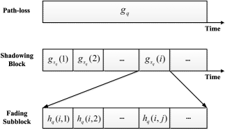
For illustrations, we provide the channel model in Fig. 2, where time axis is divided into blocks and each block consists of multiple subblocks. In particular, gqsubscript𝑔𝑞g_{q} remains constant all the time with a given dqsubscript𝑑𝑞d_{q}, gsqsubscript𝑔subscript𝑠𝑞g_{s_{q}} (q=0, 1𝑞01q=0,\ 1) remains constant within each block (i𝑖i) and varies independently among different blocks, and hqsubscript𝑞h_{q} (q=0, 1𝑞01q=0,\ 1) remains constant within each subblock (i,j𝑖𝑗i,j) and varies among different subblocks.
Refer to caption
Figure 2: Channel model, where time axis is divided into blocks and each blocks consists of multiple subblocks. In particular, gqsubscript𝑔𝑞g_{q} remains constant all the time with a given dqsubscript𝑑𝑞d_{q}, gsqsubscript𝑔subscript𝑠𝑞g_{s_{q}} (q=0, 1𝑞01q=0,\ 1) remains constant within each block (i𝑖i) and varies independently among different blocks, and hqsubscript𝑞h_{q} (q=0, 1𝑞01q=0,\ 1) remains constant within each subblock (i,j𝑖𝑗i,j) and varies among different subblocks.

II-B Signal Model

II-B1 Signal model from the MBS to the MU

Denote xmsubscript𝑥𝑚x_{m} as the MBS signal with unit power, i.e., |x0|2=1superscriptsubscript𝑥021|x_{0}|^{2}=1. If the MBS transmits the signal with power p0subscript𝑝0p_{0}, the received signal at the MU is

y0(i,j)=h0(i,j)g0gs0(i)p0(i,j)x0(i,j)+n0(i,j),subscript𝑦0𝑖𝑗subscript0𝑖𝑗subscript𝑔0subscript𝑔subscript𝑠0𝑖subscript𝑝0𝑖𝑗subscript𝑥0𝑖𝑗subscript𝑛0𝑖𝑗y_{0}(i,j)=h_{0}(i,j)\sqrt{g_{0}g_{s_{0}}(i)p_{0}(i,j)}x_{0}(i,j)+n_{0}(i,j), (3)

where (i)𝑖(i) denotes the index of the i𝑖ith block, (i,j)𝑖𝑗(i,j) represents the index of the j𝑗jth subblock in the i𝑖ith block, n0subscript𝑛0n_{0} represents the AWGN at the MU with zero mean and variance σ2superscript𝜎2\sigma^{2}. Then, the SNR of the received signal at the MU is

γ0(i,j)=|h0(i,j)|2g0gs0(i)p0(i,j)σ2.subscript𝛾0𝑖𝑗superscriptsubscript0𝑖𝑗2subscript𝑔0subscript𝑔subscript𝑠0𝑖subscript𝑝0𝑖𝑗superscript𝜎2\gamma_{0}(i,j)=\frac{|h_{0}(i,j)|^{2}g_{0}g_{s_{0}}(i)p_{0}(i,j)}{\sigma^{2}}. (4)

We further consider that the MBS and the MU adopt close loop power control (CLPC) to provide QoS guaranteed wireless communication [11]. That is, the MBS automatically adjusts its transmit power to meet a certain target SNR γTsubscript𝛾𝑇\gamma_{T} at the MU. Then, MBS’s transmit power is

p0(i,j)=γTσ2|h0(i,j)|2g0gs0(i).subscript𝑝0𝑖𝑗subscript𝛾𝑇superscript𝜎2superscriptsubscript0𝑖𝑗2subscript𝑔0subscript𝑔subscript𝑠0𝑖p_{0}(i,j)=\frac{{\gamma_{T}\sigma^{2}}}{{|h_{0}(i,j)|^{2}{g_{0}g_{s_{0}}(i)}}}. (5)

II-B2 Signal model from the MBS to the SBS

In the meantime, the received MBS signal at the SBS is

y1(i,j)=h1(i,j)g1gs1(i)p0(i,j)x0(i,j)+n1(i,j),subscript𝑦1𝑖𝑗subscript1𝑖𝑗subscript𝑔1subscript𝑔subscript𝑠1𝑖subscript𝑝0𝑖𝑗subscript𝑥0𝑖𝑗subscript𝑛1𝑖𝑗y_{1}(i,j)=h_{1}(i,j)\sqrt{{g_{1}}{g_{s_{1}}(i)}{p_{0}(i,j)}}{x_{0}}(i,j)+n_{1}(i,j), (6)

where n1subscript𝑛1n_{1} is the AWGN at the SBS with zero mean and variance σ2superscript𝜎2\sigma^{2}. Then, the SNR of the received MBS signal at the SBS is

γ1(i,j)=|h1(i,j)|2g1gs1(i)p0(i,j)σ2.subscript𝛾1𝑖𝑗superscriptsubscript1𝑖𝑗2subscript𝑔1subscript𝑔subscript𝑠1𝑖subscript𝑝0𝑖𝑗superscript𝜎2\gamma_{1}(i,j)=\frac{{|h_{1}(i,j)|^{2}{g_{1}}{g_{s_{1}}(i)}{p_{0}(i,j)}}}{{\sigma^{2}}}. (7)

By Substituting (2) and (5) into (7), γ1(i,j)subscript𝛾1𝑖𝑗\gamma_{1}(i,j) in (7) can be rewritten as

γ1(i,j)=γTd13.76d03.76gs1(i)gs0(i)|h1(i,j)|2|h0(i,j)|2.subscript𝛾1𝑖𝑗subscript𝛾𝑇superscriptsubscript𝑑13.76superscriptsubscript𝑑03.76subscript𝑔subscript𝑠1𝑖subscript𝑔subscript𝑠0𝑖superscriptsubscript1𝑖𝑗2superscriptsubscript0𝑖𝑗2{\gamma_{1}}(i,j)=\frac{{{\gamma_{T}}{d_{1}^{-3.76}}}}{{{d_{0}^{-3.76}}}}\frac{g_{s_{1}}(i)}{g_{s_{0}}(i)}\frac{{|h_{1}(i,j)|^{2}}}{{|h_{0}(i,j)|^{2}}}. (8)

III Median Based (MB) Estimator

In this section, we will develop a MB estimator to obtain the distance d0subscript𝑑0d_{0} between the MBS and the MU. In what follows, we provide the basic principle of the estimator followed by the estimator design.

III-A Basic Principle

From (8), each SNR of the received MBS signal at the SBS is highly related to the distance d0subscript𝑑0d_{0}. Then, it is possible for the SBS to measure the SNR of the received MBS signal and estimate d0subscript𝑑0d_{0}. However, it is difficult to obtain d0subscript𝑑0d_{0} directly. This is because, each SNR is also affected by random Rayleigh fadings and shadowing attenuations, and varies independently among different blocks and/or subblocks. Alternatively, the SBS can measure different SNRs of MBS signals in multiple blocks and utilize the distribution knowledge of the Rayleigh fadings and shadowing attenuations to estimate d0subscript𝑑0d_{0}.

Next, we will first calculate the cumulative density function (CDF) of the SNR at the SBS. Then, we study the relation between the CDF of the SNR at the SBS and the distance d0subscript𝑑0d_{0}. Finally, we develop the MB estimator.

III-B CDF of the SNR at the SBS

Removing the time index of the SNR at the SBS in (8) and rewriting the SNR in dB, we have

γ1,dB=γT,dB+37.6log10(d0d1)+Θr+Θs,subscript𝛾1𝑑𝐵subscript𝛾𝑇𝑑𝐵37.6subscript10subscript𝑑0subscript𝑑1subscriptΘ𝑟subscriptΘ𝑠\displaystyle{\gamma_{1,dB}}={\gamma_{T,dB}}+37.6{\log_{10}}\left(\frac{d_{0}}{d_{1}}\right)+\Theta_{r}+\Theta_{s},

where Θr=10log10(h12h02)subscriptΘ𝑟10subscript10superscriptsubscript12superscriptsubscript02{\Theta_{r}}=10{\log_{10}}\left({\frac{{h_{1}^{2}}}{{h_{0}^{2}}}}\right) and Θs=10log10(gs1)10log10(gs0)subscriptΘ𝑠10subscript10subscript𝑔subscript𝑠110subscript10subscript𝑔subscript𝑠0{\Theta_{s}}=10{\log_{10}}\left({{g_{s_{1}}}}\right)-10{\log_{10}}\left({{g_{s_{0}}}}\right). Next, we first calculate the probability density function (PDF) of ΘrsubscriptΘ𝑟\Theta_{r} and ΘssubscriptΘ𝑠\Theta_{s}, and then obtain the CDF of γ1,dBsubscript𝛾1𝑑𝐵\gamma_{1,dB}.

On one hand, both |h0|subscript0|h_{0}| amd |h1|subscript1|h_{1}| follow a Rayleigh distribution with unit mean, the CDF of ϕ=|h1|2/|h0|2italic-ϕsuperscriptsubscript12superscriptsubscript02\phi=|h_{1}|^{2}/|h_{0}|^{2} is [12]

FΦ(ϕ)=ϕ1+ϕ.subscript𝐹Φitalic-ϕitalic-ϕ1italic-ϕF_{\Phi}(\phi)=\frac{{\phi}}{{{{1+\phi}}}}. (9)

Then, the CDF of Θr=10log10(ϕ)subscriptΘ𝑟10subscript10italic-ϕ\Theta_{r}=10\log_{10}(\phi) is

FΘr(θr)=subscript𝐹subscriptΘ𝑟subscript𝜃𝑟absent\displaystyle F_{\Theta_{r}}(\theta_{r})= Pr{10log10(ϕ)θr}Pr10subscript10italic-ϕsubscript𝜃𝑟\displaystyle\Pr\left\{10\log_{10}(\phi)\leq\theta_{r}\right\}
=\displaystyle= Pr{ϕ10θr10}Pritalic-ϕsuperscript10subscript𝜃𝑟10\displaystyle\Pr\left\{\phi\leq 10^{\frac{\theta_{r}}{10}}\right\}
=\displaystyle= FΦ(10θr10).subscript𝐹Φsuperscript10subscript𝜃𝑟10\displaystyle F_{\Phi}\left(10^{\frac{\theta_{r}}{10}}\right). (10)

Substituting (9) into (10), we have the CDF of ΘrsubscriptΘ𝑟\Theta_{r} as

FΘr(θr)=11+10θr10.subscript𝐹subscriptΘ𝑟subscript𝜃𝑟11superscript10subscript𝜃𝑟10F_{\Theta_{r}}(\theta_{r})=\frac{1}{1+10^{-\frac{\theta_{r}}{10}}}. (11)

Taking the derivation of FΘr(θr)subscript𝐹subscriptΘ𝑟subscript𝜃𝑟F_{\Theta_{r}}(\theta_{r}), we have the PDF of ΘrsubscriptΘ𝑟\Theta_{r} as

fΘr(θr)=ln1010θr1010(1+10θr10)2.subscript𝑓subscriptΘ𝑟subscript𝜃𝑟10superscript10subscript𝜃𝑟1010superscript1superscript10subscript𝜃𝑟102{f_{{\Theta_{r}}}}\left({{\theta_{r}}}\right)=\frac{{\ln 10\cdot{{10}^{-\frac{{{\theta_{r}}}}{{10}}}}}}{{10{{\left({1+{{10}^{-\frac{{{\theta_{r}}}}{{10}}}}}\right)}^{2}}}}. (12)

On the other hand, both gs0subscript𝑔subscript𝑠0g_{s_{0}} and gs1subscript𝑔subscript𝑠1g_{s_{1}} follow a log-normal distribution with variance σs2superscriptsubscript𝜎𝑠2\sigma_{s}^{2}. Then, it is straightforward to obtain that ΘssubscriptΘ𝑠\Theta_{s} follows a normal distribution with zero means and variance 2σs22superscriptsubscript𝜎𝑠22\sigma_{s}^{2}. Thus, the PDF of ΘssubscriptΘ𝑠\Theta_{s} is

fΘs(θs)=14πσs2eθs24σs2.subscript𝑓subscriptΘ𝑠subscript𝜃𝑠14𝜋superscriptsubscript𝜎𝑠2superscript𝑒superscriptsubscript𝜃𝑠24superscriptsubscript𝜎𝑠2{f_{{\Theta_{s}}}}\left({{\theta_{s}}}\right)=\frac{1}{{\sqrt{4\pi\sigma_{s}^{2}}}}{e^{-\frac{{{{{{\theta_{s}}}}^{2}}}}{{4{\sigma_{s}^{2}}}}}}. (13)

Note that, the CDF of γ1,dBsubscript𝛾1𝑑𝐵\gamma_{1,dB} is

FΓ1,dB(γ1,dB)subscript𝐹subscriptΓ1𝑑𝐵subscript𝛾1𝑑𝐵\displaystyle F_{\Gamma_{1,dB}}(\gamma_{1,dB})
=\displaystyle= Pr{γT,dB+37.6log10(d0d1)+Θr+Θsγ1,dB}Prsubscript𝛾𝑇𝑑𝐵37.6subscript10subscript𝑑0subscript𝑑1subscriptΘ𝑟subscriptΘ𝑠subscript𝛾1𝑑𝐵\displaystyle\Pr\left\{{\gamma_{T,dB}}+37.6{\log_{10}}\left(\frac{d_{0}}{d_{1}}\right)+{\Theta_{r}}+{\Theta_{s}}\leq\gamma_{1,dB}\right\}
=\displaystyle= Pr{Θr+Θsγ1,dBγT,dB37.6log10(d0d1)}.PrsubscriptΘ𝑟subscriptΘ𝑠subscript𝛾1𝑑𝐵subscript𝛾𝑇𝑑𝐵37.6subscript10subscript𝑑0subscript𝑑1\displaystyle\Pr\left\{{\Theta_{r}}\!+{\Theta_{s}}\leq\gamma_{1,dB}\!-{\gamma_{T,dB}}\!-37.6{\log_{10}}\left(\frac{d_{0}}{d_{1}}\right)\right\}. (14)

If we denote m(γ1,dB)=γ1,dBγT,dB37.6log10(d0d1)𝑚subscript𝛾1𝑑𝐵subscript𝛾1𝑑𝐵subscript𝛾𝑇𝑑𝐵37.6subscript10subscript𝑑0subscript𝑑1m(\gamma_{1,dB})=\gamma_{1,dB}-{\gamma_{T,dB}}-37.6{\log_{10}}\left(\frac{d_{0}}{d_{1}}\right), the CDF of γ1,dBsubscript𝛾1𝑑𝐵\gamma_{1,dB} in (III-B) can be calculated as

FΓ1,dB(γ1,dB)=subscript𝐹subscriptΓ1𝑑𝐵subscript𝛾1𝑑𝐵absent\displaystyle F_{\Gamma_{1,dB}}(\gamma_{1,dB})= Pr{Θr+Θsm(γ1,dB)}PrsubscriptΘ𝑟subscriptΘ𝑠𝑚subscript𝛾1𝑑𝐵\displaystyle\Pr\left\{{\Theta_{r}}+{\Theta_{s}}\leq m(\gamma_{1,dB})\right\}
=\displaystyle= m(γ1,dB)θsfΘs(θs)fΘr(θr)𝑑θr𝑑θssuperscriptsubscriptsuperscriptsubscript𝑚subscript𝛾1𝑑𝐵subscript𝜃𝑠subscript𝑓subscriptΘ𝑠subscript𝜃𝑠subscript𝑓subscriptΘ𝑟subscript𝜃𝑟differential-dsubscript𝜃𝑟differential-dsubscript𝜃𝑠\displaystyle\int_{-\infty}^{\infty}\int_{-\infty}^{m(\gamma_{1,dB})-{\theta_{s}}}\!\!f_{\Theta_{s}}\left(\theta_{s}\right)\!\!f_{\Theta_{r}}\left(\theta_{r}\right)d\theta_{r}d\theta_{s}
=\displaystyle\!=\! fΘs(θs)FΘr(m(γ1,dB)θs)𝑑θs.superscriptsubscriptsubscript𝑓subscriptΘ𝑠subscript𝜃𝑠subscript𝐹subscriptΘ𝑟𝑚subscript𝛾1𝑑𝐵subscript𝜃𝑠differential-dsubscript𝜃𝑠\displaystyle\int_{-\infty}^{\infty}\!\!f_{\Theta_{s}}\left(\theta_{s}\right)F_{\Theta_{r}}\left(m(\gamma_{1,dB})\!-\!{\theta_{s}}\!\right)d\theta_{s}. (15)

III-C Relations between the CDF of γ1,dBsubscript𝛾1𝑑𝐵\gamma_{1,dB} and the Distance d0subscript𝑑0d_{0}

To begin with, we provide the definition of the median x12subscript𝑥12x_{\frac{1}{2}} of a random variable X𝑋X as follows,

Definition 1

For a random variable X𝑋X with CDF FX(x)subscript𝐹𝑋𝑥F_{X}(x), x𝑥x\in\mathbb{R}, if x12subscript𝑥12x_{\frac{1}{2}} satisfies both FX(x12)=Pr{Xx12}=12subscript𝐹𝑋subscript𝑥12Pr𝑋subscript𝑥1212F_{X}(x_{\frac{1}{2}})=\Pr\{X\leq x_{\frac{1}{2}}\}=\frac{1}{2} and 1FX(x12)=Pr{Xx12}=121subscript𝐹𝑋subscript𝑥12Pr𝑋subscript𝑥12121-F_{X}(x_{\frac{1}{2}})=\Pr\{X\geq x_{\frac{1}{2}}\}=\frac{1}{2}, x12subscript𝑥12x_{\frac{1}{2}} is defined as the median of the random variable X𝑋X.

Based on Definition 1, we can obtain the median γ1,dB,12subscript𝛾1𝑑𝐵12\gamma_{1,dB,\frac{1}{2}} of the random variable γ1,dBsubscript𝛾1𝑑𝐵\gamma_{1,dB} by letting FΓ1,dB(γ1,dB)subscript𝐹subscriptΓ1𝑑𝐵subscript𝛾1𝑑𝐵F_{\Gamma_{1,dB}}\left(\gamma_{1,dB}\right) in (III-B) be 1212\frac{1}{2}, i.e.,

fΘs(θs)FΘr(m(γ1,dB,12)θs)𝑑θs=12.superscriptsubscriptsubscript𝑓subscriptΘ𝑠subscript𝜃𝑠subscript𝐹subscriptΘ𝑟𝑚subscript𝛾1𝑑𝐵12subscript𝜃𝑠differential-dsubscript𝜃𝑠12\displaystyle\int_{-\infty}^{\infty}f_{\Theta_{s}}\left(\theta_{s}\right)F_{\Theta_{r}}\left(m(\gamma_{1,dB,\frac{1}{2}})-{\theta_{s}}\right)d\theta_{s}=\frac{1}{2}. (16)

Then, we have the following Theorem.

Theorem 1

The median γ1,dB,12subscript𝛾1𝑑𝐵12\gamma_{1,dB,\frac{1}{2}} enables m(γ1,dB,12)=0𝑚subscript𝛾1𝑑𝐵120m(\gamma_{1,dB,\frac{1}{2}})=0 to hold.

Proof:

The detailed proof of this Theorem is provided in the Appendix. ∎

Theorem 1 indicates that the relation between the median γ1,dB,12subscript𝛾1𝑑𝐵12\gamma_{1,dB,\frac{1}{2}} and the distance d0subscript𝑑0d_{0} satisfies

m(γ1,dB,12)=γ1,dB,12γT,dB37.6log10(d0d1)=0.𝑚subscript𝛾1𝑑𝐵12subscript𝛾1𝑑𝐵12subscript𝛾𝑇𝑑𝐵37.6subscript10subscript𝑑0subscript𝑑10\displaystyle m(\gamma_{1,dB,\frac{1}{2}})\!=\!\gamma_{1,dB,\frac{1}{2}}\!-\!{\gamma_{T,dB}}\!-\!37.6{\log_{10}}\left(\frac{d_{0}}{d_{1}}\right)=0. (17)

Thus, if γ1,dB,12subscript𝛾1𝑑𝐵12\gamma_{1,dB,\frac{1}{2}} is available at the SBS, d0subscript𝑑0d_{0} can be directly calculated with (17). However, γ1,dB,12subscript𝛾1𝑑𝐵12\gamma_{1,dB,\frac{1}{2}} is unknown to the SBS in practical situations. To deal with this issue, we will first estimate γ1,dB,12subscript𝛾1𝑑𝐵12\gamma_{1,dB,\frac{1}{2}} and then obtain the estimation of d0subscript𝑑0d_{0} with (17).

III-D Estimator Design

We first give the definition of the sample median x12ssubscriptsuperscript𝑥𝑠12x^{s}_{\frac{1}{2}} of a random variable X𝑋X as follows,

Definition 2

For a random variable X𝑋X with samples xmsubscript𝑥𝑚x_{m} (1mM1𝑚𝑀1\leq m\leq M), if x12ssubscriptsuperscript𝑥𝑠12x^{s}_{\frac{1}{2}} satisfies both Pr{xmx12s}=12Prsubscript𝑥𝑚subscriptsuperscript𝑥𝑠1212\Pr\{x_{m}\leq x^{s}_{\frac{1}{2}}\}=\frac{1}{2} and Pr{xmx12s}=12Prsubscript𝑥𝑚subscriptsuperscript𝑥𝑠1212\Pr\{x_{m}\geq x^{s}_{\frac{1}{2}}\}=\frac{1}{2}, x12ssubscriptsuperscript𝑥𝑠12x^{s}_{\frac{1}{2}} is defined as the sample median of the random variable X𝑋X.

If the SBS observes MBS signals in I𝐼I blocks and measures γ1,dBsubscript𝛾1𝑑𝐵\gamma_{1,dB} of J𝐽J subblocks within each block, the SBS is able to measure K=IJ𝐾𝐼𝐽K=IJ independent samples of γ1,dBsubscript𝛾1𝑑𝐵\gamma_{1,dB}, namely, γ1,dB(i,j)subscript𝛾1𝑑𝐵𝑖𝑗\gamma_{1,dB}(i,j) (1iI1𝑖𝐼1\leq i\leq I, 1jJ1𝑗𝐽1\leq j\leq J). In what follows, we will approximate the median γ1,dB,12subscript𝛾1𝑑𝐵12\gamma_{1,dB,\frac{1}{2}} with the sample median γ1,dB,12ssubscriptsuperscript𝛾𝑠1𝑑𝐵12\gamma^{s}_{1,dB,\frac{1}{2}} of these K𝐾K samples. Then, by substituting the approximated γ1,dB,12subscript𝛾1𝑑𝐵12\gamma_{1,dB,\frac{1}{2}} into (17), we obtain the estimation of d0subscript𝑑0d_{0}.

To begin with, by sorting the K𝐾K samples in ascending order, the K𝐾K samples can be relabelled as γ¯1,dB(k)subscript¯𝛾1𝑑𝐵𝑘\bar{\gamma}_{1,dB}(k) (1kK1𝑘𝐾1\leq k\leq K), i.e., γ¯1,dB(k1)γ¯1,dB(k2)subscript¯𝛾1𝑑𝐵subscript𝑘1subscript¯𝛾1𝑑𝐵subscript𝑘2\bar{\gamma}_{1,dB}(k_{1})\leq\bar{\gamma}_{1,dB}(k_{2}) for 1k1k2K1subscript𝑘1subscript𝑘2𝐾1\leq k_{1}\leq k_{2}\leq K. Since the sample medians γ¯1,dB,12ssubscriptsuperscript¯𝛾𝑠1𝑑𝐵12\bar{\gamma}^{s}_{1,dB,\frac{1}{2}} of these K𝐾K samples for odd and even K𝐾K can be different, we will develop the MB estimator for odd and even K𝐾K separately.

III-D1 For the case that K𝐾K is odd

When K𝐾K is odd, the sample median is γ1,dB,12s=γ¯1,dB(K+12)subscriptsuperscript𝛾𝑠1𝑑𝐵12subscript¯𝛾1𝑑𝐵𝐾12\gamma^{s}_{1,dB,\frac{1}{2}}=\bar{\gamma}_{1,dB}\left(\frac{K+1}{2}\right). Then, the median of γ1,dBsubscript𝛾1𝑑𝐵\gamma_{1,dB} can be approximated as

γ1,dB,12γ¯1,dB(K+12).subscript𝛾1𝑑𝐵12subscript¯𝛾1𝑑𝐵𝐾12\gamma_{1,dB,\frac{1}{2}}\approx\bar{\gamma}_{1,dB}\left(\frac{K+1}{2}\right). (18)

By substituting (18) into (17), we have the MB estimator as

d^0=d110γ¯1,dB(K+12)γT,dB37.6.subscript^𝑑0subscript𝑑1superscript10subscript¯𝛾1𝑑𝐵𝐾12subscript𝛾𝑇𝑑𝐵37.6\begin{split}{{\hat{d}}_{0}}=d_{1}10^{\frac{\bar{\gamma}_{1,dB}\left(\frac{K+1}{2}\right)-\gamma_{T,dB}}{37.6}}.\end{split} (19)

III-D2 For the case that K𝐾K is even

When K𝐾K is even, the sample median is between γ¯1,dB(K2)subscript¯𝛾1𝑑𝐵𝐾2\bar{\gamma}_{1,dB}\left(\frac{K}{2}\right) and γ¯1,dB(K2+1)subscript¯𝛾1𝑑𝐵𝐾21\bar{\gamma}_{1,dB}\left(\frac{K}{2}+1\right). Then, the median of γ1,dBsubscript𝛾1𝑑𝐵\gamma_{1,dB} can be approximated as

γ1,dB,12γ¯1,dB(K2)+γ¯1,dB(K2+1)2.subscript𝛾1𝑑𝐵12subscript¯𝛾1𝑑𝐵𝐾2subscript¯𝛾1𝑑𝐵𝐾212\gamma_{1,dB,\frac{1}{2}}\approx\frac{\bar{\gamma}_{1,dB}\left(\frac{K}{2}\right)+\bar{\gamma}_{1,dB}\left(\frac{K}{2}+1\right)}{2}. (20)

By substituting (20) into (17), we have the MB estimator as

d^0=d110γ¯1,dB(K2)+γ¯1,dB(K2+1)2γT,dB37.6.subscript^𝑑0subscript𝑑1superscript10subscript¯𝛾1𝑑𝐵𝐾2subscript¯𝛾1𝑑𝐵𝐾212subscript𝛾𝑇𝑑𝐵37.6\begin{split}{{\hat{d}}_{0}}=d_{1}10^{\frac{\frac{\bar{\gamma}_{1,dB}\left(\frac{K}{2}\right)+\bar{\gamma}_{1,dB}\left(\frac{K}{2}+1\right)}{2}-\gamma_{T,dB}}{37.6}}.\end{split} (21)

Consequently, the MB estimator can be summarized as

d^0={d110γ¯1,dB(K+12)γT,dB37.6,forKisodd,d110γ¯1,dB(K2)+γ¯1,dB(K2+1)2γT,dB37.6,forKiseven.subscript^𝑑0casessubscript𝑑1superscript10subscript¯𝛾1𝑑𝐵𝐾12subscript𝛾𝑇𝑑𝐵37.6for𝐾isodd,subscript𝑑1superscript10subscript¯𝛾1𝑑𝐵𝐾2subscript¯𝛾1𝑑𝐵𝐾212subscript𝛾𝑇𝑑𝐵37.6for𝐾iseven{{\hat{d}}_{0}}\!=\!\left\{\!\!\begin{array}[]{l}d_{1}10^{\frac{\bar{\gamma}_{1,dB}\left(\frac{K+1}{2}\right)-\gamma_{T,dB}}{37.6}},\quad\quad\quad\quad\ \ \text{for}\ K\ \text{is}\ \text{odd,}\\ d_{1}10^{\frac{\frac{\bar{\gamma}_{1,dB}\left(\frac{K}{2}\right)+\bar{\gamma}_{1,dB}\left(\frac{K}{2}+1\right)}{2}-\gamma_{T,dB}}{37.6}},\ \text{for}\ K\ \text{is}\ \text{even}.\end{array}\right. (22)

From (22), the MB estimator d^0subscript^𝑑0\hat{d}_{0} is determined by the target SNR γT,dBsubscript𝛾𝑇𝑑𝐵\gamma_{T,dB} at the MU, the distance d1subscript𝑑1d_{1} between the MBS and the SBS, and the SNR γ1,dBsubscript𝛾1𝑑𝐵\gamma_{1,dB} of the MBS signal at the SBS. Note that, γT,dBsubscript𝛾𝑇𝑑𝐵\gamma_{T,dB} can be obtained by the SBS through observing the modulation and coding scheme (MCS) of the MBS signal [13]. d1subscript𝑑1d_{1} is available at the SBS. γ1,dBsubscript𝛾1𝑑𝐵\gamma_{1,dB} is measured at the SBS and also known to the SBS. Therefore, the estimation of d0subscript𝑑0d_{0} can be directly calculated with (22). In other words, the computational complexity of the MB estimator in (22) is O(1)𝑂1O(1).

III-E Estimation Performance Analysis

In this part, we present the estimation performance analysis of the MB estimator in Theorem 1.

Theorem 2

With the MB estimator in (22), g0subscript𝑔0g_{0} can be bounded by

d110γc,dB(IJ+121)γT,dB37.6d0d110γc,dB(IJ+12+1)γT,dB37.6subscript𝑑1superscript10subscript𝛾𝑐𝑑𝐵𝐼𝐽121subscript𝛾𝑇𝑑𝐵37.6subscript𝑑0subscript𝑑1superscript10subscript𝛾𝑐𝑑𝐵𝐼𝐽121subscript𝛾𝑇𝑑𝐵37.6\!d_{1}10^{\frac{\gamma_{c,dB}\left(\left\lceil\frac{IJ+1}{2}\right\rceil-1\right)-\gamma_{T,dB}}{37.6}}\!\!\leq\!d_{0}\!\leq\!\!d_{1}10^{\frac{\gamma_{c,dB}\left(\left\lfloor\frac{IJ+1}{2}\right\rfloor+1\right)-\gamma_{T,dB}}{37.6}}\! (23)

with probability (1(12)[K2+1])2superscript1superscript12delimited-[]𝐾212\left(1-\left({\frac{1}{2}}\right)^{\left[\frac{K}{2}+1\right]}\right)^{2}, where x𝑥\lceil x\rceil denotes the smallest integer that is no smaller than x𝑥x, x𝑥\lfloor x\rfloor denotes the largest integer that is no larger than x𝑥x, and [x]delimited-[]𝑥[x] rounds x𝑥x to the nearest integer.

Theorem 2 indicates that d0subscript𝑑0d_{0} can be upper bounded and lower bounded by functions of the measured SNRs at the SBS with a certain probability. In particular, the probability is a function of the number of the sensed primary signals, i.e., IJ𝐼𝐽IJ. For instance, we consider I=12𝐼12I=12 and J=1𝐽1J=1, the bounds of d0subscript𝑑0d_{0} in (23) holds with probability larger than 98%percent9898\%. As IJ𝐼𝐽IJ increases, d0subscript𝑑0d_{0} can be almost surely bounded with (23).
Refer to caption
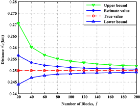
Figure 3: Estimation accuracy of the MB estimator versus the number of blocks, i.e., I𝐼I. In particular, we set J=1𝐽1J=1.

In Fig. 3, we illustrate estimation accuracy of the MB estimator versus the number of blocks, i.e., I𝐼I. In particular, we provide the true value of the channel gain d0subscript𝑑0d_{0}, the estimation d^0subscript^𝑑0\hat{d}_{0} with the MB estimation, the upper bound and the lower bound in (23). Here, the distance between the MBS and the MU is d0=0.25subscript𝑑00.25d_{0}=0.25 km, and the distance between the MBS and the MU is d1=0.1subscript𝑑10.1d_{1}=0.1 km. From this figure, we observe that the estimation value d^0subscript^𝑑0\hat{d}_{0} is strictly upper bounded and lower bounded by the results in Theorem 1. Besides, both the upper bound and the lower bound converge to d0subscript𝑑0d_{0} and d^0subscript^𝑑0\hat{d}_{0}. This means a larger I𝐼I leads to a more accurate estimation as well as tighter upper and lower bounds. Furthermore, we observe that the estimated value d^0subscript^𝑑0\hat{d}_{0} converges to the true value of the channel gain d0subscript𝑑0d_{0} as I𝐼I increases.

IV Numerical results

In this section, we provide the numerical results to demonstrate the performance of the proposed MB estimator. Here, we adopt the system model as in Section II, where the radius of the MBS’s coverage is R=0.5𝑅0.5R=0.5 km, the power of the AWGN σ2=114superscript𝜎2114\sigma^{2}=-114 dBm, the target SNR of the MU is γT=10subscript𝛾𝑇10\gamma_{T}=10 dB. Furthermore, 104superscript10410^{4} Monte Carlo trails are conducted for each curve. To begin with, we define the estimation error of d0subscript𝑑0d_{0} as ϵ=|d^0d0d0|italic-ϵsubscript^𝑑0subscript𝑑0subscript𝑑0\epsilon=|\frac{\hat{d}_{0}-d_{0}}{d_{0}}|.

Refer to caption
Figure 4: The estimation error with different I𝐼I and/or J𝐽J. In particular, we set d0=0.25subscript𝑑00.25d_{0}=0.25 km and d1=0.1subscript𝑑10.1d_{1}=0.1 km.

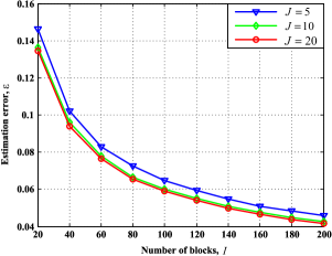
Fig. 4 investigates the impact of K=IJ𝐾𝐼𝐽K=IJ on the the estimation error. In particular, we set d0=0.25subscript𝑑00.25d_{0}=0.25 km and d1=0.1subscript𝑑10.1d_{1}=0.1 km. From this figure, the estimation error decreases as J𝐽J (I𝐼I) grows. This is reasonable, a larger J𝐽J (I𝐼I) leads to more SNR samples at the SBS and provides more accurate information of the median of the SNRs at the SBS. By using the relation between the median of the SNRs at the SBS and the distance d0subscript𝑑0d_{0}, the MB estimator is able to output a more accurate estimation of d0subscript𝑑0d_{0}. Besides, we observe that a small increase of I𝐼I leads to big jump of the estimation error, while a large increase of I𝐼I results in a slight decrease of the estimation error. This indicates that the estimation error is more sensitive to I𝐼I than J𝐽J. Thus, It is an effective way to achieve a small estimation error by adopting a large I𝐼I and a reasonable J𝐽J.

Refer to caption
Figure 5: The average measured SNR at the SBS when the MU and/or the SBS are in different locations, i.e., different d0subscript𝑑0d_{0} and/or d1subscript𝑑1d_{1}. In particular, we set I=200𝐼200I=200 and J=20𝐽20J=20.

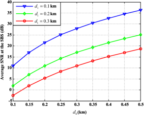
Fig. 5 provides the average measured SNRs at the SBS when the MU and/or the SBS are in different locations, i.e., different d0subscript𝑑0d_{0} and/or d1subscript𝑑1d_{1}. In general, the SNR at the SBS increases as d0subscript𝑑0d_{0} grows or d1subscript𝑑1d_{1} decreases. On one hand, for a given target SNR of the received signals at the MU, a larger d0subscript𝑑0d_{0} requires a larger transmit power at the MBS to satisfy the target SNR. This leads to a stronger received signal at the SBS and outputs a larger SNR. On the other hand, a smaller d1subscript𝑑1d_{1} also enables the SBS to receive a stronger signal from the MBS and contributes to a larger SNR at the SBS.
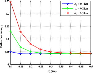
Refer to caption
Figure 6: The estimation error when the MU and/or the SBS are in different locations, i.e., different d0subscript𝑑0d_{0} and/or d1subscript𝑑1d_{1}. In particular, we set I=200𝐼200I=200 and J=20𝐽20J=20.

Fig. 6 provides the estimation error when the MU and/or the SBS are in different locations, i.e., different d0subscript𝑑0d_{0} and/or d1subscript𝑑1d_{1}. From this figure, the estimation error decreases as d0subscript𝑑0d_{0} increases or d1subscript𝑑1d_{1} decreases. Note that, both the increase of d0subscript𝑑0d_{0} and the decrease of d1subscript𝑑1d_{1} enhances the average SNR at the SBS from the results in Fig. 5. This reduces the measure error of each SNR at the SBS. By adopting these SNRs to estimate the distance d0subscript𝑑0d_{0}, the estimation error is also reduced. Besides, we observe that the estimation error converges to around 4%percent44\% as d0subscript𝑑0d_{0} increases or d1subscript𝑑1d_{1} decreases. In addition, by comparing Fig. 5 and Fig. 6, we have the estimation error of d0subscript𝑑0d_{0} with different average SNRs at the SBS as in Table I. In fact, the estimation error in Table I can be further reduced by increasing I𝐼I and J𝐽J from the results in Fig. 4. Therefore, we can select a proper I𝐼I and J𝐽J to obtain an acceptable estimation performance in practical situations.

Table I: Estimation error of d0subscript𝑑0d_{0} with different average SNRs at the SBS.
Average γ1,dBsubscript𝛾1𝑑𝐵\gamma_{1,dB} 0 5 10 15 20 \cdots
ϵitalic-ϵ\epsilon 16% 8% 5% 4.5% 4% 4%

V Conclusions

In this paper, we studied the coexistence problem between a macro cell and a small cell in an underlay HetNet. In particular, we proposed a MB estimator for the SBS to estimate the distance between the MBS and the MU. Different from the conventional approach, the MB estimator does not require any backhaul link from the macro system to the SBS. With the distance information, the SBS is able to manage the interference to the MU and achieve the coexistence. Numerical results showed that the estimation error of the MB estimator can be as small as 4%percent44\%.

VI Appendix

To prove Theorem 1, we only need to verify fΘs(θs)FΘr(θs)𝑑θs=12superscriptsubscriptsubscript𝑓subscriptΘ𝑠subscript𝜃𝑠subscript𝐹subscriptΘ𝑟subscript𝜃𝑠differential-dsubscript𝜃𝑠12\int_{-\infty}^{\infty}f_{\Theta_{s}}\left(\theta_{s}\right)F_{\Theta_{r}}\left(-{\theta_{s}}\right)d\theta_{s}=\frac{1}{2}. Substituting (11) into fΘs(θs)FΘr(θs)𝑑θssuperscriptsubscriptsubscript𝑓subscriptΘ𝑠subscript𝜃𝑠subscript𝐹subscriptΘ𝑟subscript𝜃𝑠differential-dsubscript𝜃𝑠\int_{-\infty}^{\infty}f_{\Theta_{s}}\left(\theta_{s}\right)F_{\Theta_{r}}\left(-{\theta_{s}}\right)d\theta_{s}, we have

fΘs(θs)FΘr(θs)𝑑θssuperscriptsubscriptsubscript𝑓subscriptΘ𝑠subscript𝜃𝑠subscript𝐹subscriptΘ𝑟subscript𝜃𝑠differential-dsubscript𝜃𝑠\displaystyle\int_{-\infty}^{\infty}f_{\Theta_{s}}\left(\theta_{s}\right)F_{\Theta_{r}}\left(-{\theta_{s}}\right)d\theta_{s}
=\displaystyle= 0fΘs(θs)11+10θs10𝑑θs+0fΘs(θs)11+10θs10𝑑θssuperscriptsubscript0subscript𝑓subscriptΘ𝑠subscript𝜃𝑠11superscript10subscript𝜃𝑠10differential-dsubscript𝜃𝑠superscriptsubscript0subscript𝑓subscriptΘ𝑠subscript𝜃𝑠11superscript10subscript𝜃𝑠10differential-dsubscript𝜃𝑠\displaystyle\!\int_{-\infty}^{0}\!\!\!f_{\Theta_{s}}\!\!\left(\theta_{s}\right)\frac{1}{1\!+\!10^{\frac{\theta_{s}}{10}}}d\theta_{s}\!\!+\!\!\int_{0}^{\infty}\!\!\!f_{\Theta_{s}}\!\!\left(\theta_{s}\right)\frac{1}{1\!+\!10^{\frac{\theta_{s}}{10}}}d\theta_{s}
=\displaystyle\!= 0fΘs(θs)11+10θs10𝑑θs+0fΘs(θs)11+10θs10𝑑θs.superscriptsubscript0subscript𝑓subscriptΘ𝑠subscript𝜃𝑠11superscript10subscript𝜃𝑠10differential-dsubscript𝜃𝑠superscriptsubscript0subscript𝑓subscriptΘ𝑠subscript𝜃𝑠11superscript10subscript𝜃𝑠10differential-dsubscript𝜃𝑠\displaystyle\!\int_{0}^{\infty}\!\!\!f_{\Theta_{s}}\!\!\left(-\theta_{s}\!\right)\frac{1}{1\!+\!10^{-\frac{\theta_{s}}{10}}}d\theta_{s}\!\!+\!\!\int_{0}^{\infty}\!\!\!f_{\Theta_{s}}\!\!\left(\theta_{s}\!\right)\frac{1}{1\!+\!10^{\frac{\theta_{s}}{10}}}d\theta_{s}. (24)

From (13), we observer that fΘs(θs)subscript𝑓subscriptΘ𝑠subscript𝜃𝑠{{f_{{\Theta_{s}}}}\left({{\theta_{s}}}\right)} is an even function. Then, we have fΘs(θs)=fΘs(θs)subscript𝑓subscriptΘ𝑠subscript𝜃𝑠subscript𝑓subscriptΘ𝑠subscript𝜃𝑠f_{\Theta_{s}}\left(-\theta_{s}\right)=f_{\Theta_{s}}\left(\theta_{s}\right). Meanwhile, we have 11+10θs10=111+10θs1011superscript10subscript𝜃𝑠10111superscript10subscript𝜃𝑠10\frac{1}{1+10^{-\frac{\theta_{s}}{10}}}=1-\frac{1}{1+10^{\frac{\theta_{s}}{10}}}. Thus, (VI) can be rewritten as

fΘs(θs)FΘr(θs)𝑑θssuperscriptsubscriptsubscript𝑓subscriptΘ𝑠subscript𝜃𝑠subscript𝐹subscriptΘ𝑟subscript𝜃𝑠differential-dsubscript𝜃𝑠\displaystyle\int_{-\infty}^{\infty}f_{\Theta_{s}}\left(\theta_{s}\right)F_{\Theta_{r}}\left(-{\theta_{s}}\right)d\theta_{s}
=\displaystyle= 0fΘs(θs)(111+10θs10)𝑑θs+0fΘs(θs)11+10θs10𝑑θssuperscriptsubscript0subscript𝑓subscriptΘ𝑠subscript𝜃𝑠111superscript10subscript𝜃𝑠10differential-dsubscript𝜃𝑠superscriptsubscript0subscript𝑓subscriptΘ𝑠subscript𝜃𝑠11superscript10subscript𝜃𝑠10differential-dsubscript𝜃𝑠\displaystyle\int_{0}^{\infty}\!\!\!f_{\Theta_{s}}\left(\theta_{s}\right)\left(\!1-\!\frac{1}{1\!+\!10^{\frac{\theta_{s}}{10}}}\!\right)d\theta_{s}\!+\!\int_{0}^{\infty}\!\!\!f_{\Theta_{s}}\left(\theta_{s}\right)\frac{1}{1\!+\!10^{\frac{\theta_{s}}{10}}}d\theta_{s}
=\displaystyle= 0fΘs(θs)𝑑θssuperscriptsubscript0subscript𝑓subscriptΘ𝑠subscript𝜃𝑠differential-dsubscript𝜃𝑠\displaystyle\int_{0}^{\infty}f_{\Theta_{s}}\left(\theta_{s}\right)d\theta_{s}
=\displaystyle= 12.12\displaystyle\frac{1}{2}. (25)

Here, we complete the proof of Theorem 1.

References

  • [1] D. Liu, L. Wang, Y. Chen, M. Elkashlan, K. Wong, R. Schober, and L. Hanzo, “User Association in 5G Networks: A Survey and an Outlook,” IEEE Commun. Surveys &\& Tutorials, vol. 18, no. 2, pp. 1018-1044, Second quarter, 2016.
  • [2] Y. Lin, W. Bao, W. Yu, and B. Liang, “Optimizing User Association and Spectrum Allocation in HetNets: A Utility Perspective,” IEEE J. Select. Areas Commun., vol. 33, no. 6, pp. 1025 - 1039, Jun. 2015.
  • [3] M. Peng, C. Wang, J. Li, H. Xiang, and V. Lau, “Recent Advances in Underlay Heterogeneous Networks: Interference Control, Resource Allocation, and Self-Organization,” IEEE Commun. Surveys &\& Tutorials, vol. 17, no. 2, pp. 700-729, Second quarter, 2015.
  • [4] D. C. Chen, T. Q. S. Quek, and M. Kountouris, “Backhauling in Heterogeneous Cellular Networks: Modeling and Tradeoffs,” IEEE Trans. Wireless Commun., vol. 14, no. 6, pp. 3194-3206, Jun. 2015.
  • [5] Y. Yang, T. Q. S. Quek, and L. Duan, “Backhaul-Constrained Small Cell Networks: Refunding and QoS Provisioning,” IEEE Trans. Wirelss Commun., vol. 13, no. 9, pp. 5148-5161, Sep. 2014.
  • [6] N. Mokari, F. Alavi, S. Parsaeefard, and T. Le-Ngoc, “Limited-Feedback Resource Allocation in Heterogeneous Cellular Networks,” IEEE Trans. Veh. Technol., vol. 65, no. 4, pp. 2509-2521, Apr. 2016.
  • [7] P. Pinto, A. Giorgetti, M. Z. Win, and M. Chiani, “A Stochastic Geometry Approach to Coexistence in Heterogeneous Wireless Networks,” IEEE J. Select. Areas Commun., vol. 27, no. 7, pp. 1268-1282, Sep. 2009.
  • [8] J. G. Andrews, F. Baccelli, and R. K. Ganti, “A tractable approach to coverage and rate in cellular networks,” IEEE Trans. Commun., vol. 59, no. 11, pp. 3122-3134, Nov. 2011.
  • [9] H. ElSawy, E. Hossain, and M. Haenggi, “Stochastic Geometry for Modeling, Analysis, and Design of Multi-Tier and Cognitive Cellular Wireless Networks: A Survey,” IEEE Commun. Surveys &\& Tutorials, vol. 15, no. 3, pp. 996-1019, Third Quarter, 2013.
  • [10] 3GPP, Physical Layer Aspects for Evolved Universal Terrestrial Radio Access (UTRA), 3GPP TR 25.814, 2006.
  • [11] R. Zhang, “On active learning and supervised transmission of spectrum sharing based cognitive radios by exploiting hidden primary radio feedback,” IEEE Trans. Commun., vol. 58, no. 10, pp. 2960-2970, Oct. 2010.
  • [12] H. Kim, S. Lim, H. Wang, and D. Hong, “Optimal power allocation and outage analysis for cognitive full duplex relay systems,” IEEE Trans. Wireless Commun., vol. 11, no. 10, pp. 3754-3765, Oct. 2012.
  • [13] D. Tse and P. Viswanath, Fundamentals of wireless communications. Cambridge University Press, 2005.