Photo- with CuBAN: An improved photometric redshift estimator using Clustering aided Back Propagation Neural network
Abstract
We present an improved photometric redshift estimator code, CuBAN, that is publicly available at https://goo.gl/fpk90V. It uses the back propagation neural network along with clustering of the training set, which makes it more efficient than existing neural network codes. In CuBAN, the training set is divided into several self learning clusters with galaxies having similar photometric properties and spectroscopic redshifts within a given span. The clustering algorithm uses the color information (i.e. , etc.) rather than the apparent magnitudes at various photometric bands as the photometric redshift is more sensitive to the flux differences between different bands rather than the actual values. Separate neural networks are trained for each cluster using all possible colors, magnitudes and uncertainties in the measurements. For a galaxy with unknown redshift, we identify the closest possible clusters having similar photometric properties and use those clusters to get the photometric redshifts using the particular networks that were trained using those cluster members. For galaxies that do not match with any training cluster, the photometric redshifts are obtained from a separate network that uses entire training set. This clustering method enables us to determine the redshifts more accurately. SDSS Stripe 82 catalog has been used here for the demonstration of the code. For the clustered sources with redshift range , the residual error () in the training/testing phase is as low as 0.03 compared to the existing ANNz code that provides residual error on the same test data set of 0.05. Further, we provide a much better estimate of the uncertainty of the derived photometric redshift.
keywords:
methods: data analysis; techniques: photometric; galaxies: photometry; galaxies: distances and redshifts1 Introduction
Even though there is a huge advancement in the telescope technology, spectroscopy of a large number of galaxies is still very time expensive especially for high redshift large scale galaxy surveys. Thus photometry is still the best bet for such surveys whether they are the existing ones, i.e. Solan Digital Sky Surveys (SDSS), 2dF Galaxy redshift Survey, Blanco Cosmological Survey, Dark Energy Survey (Ahn et al., 2014; Colless, 1999; Bleem et al., 2015) or the future planed ones like Large Synoptic Survey Telescope (Ivezic et al., 2008), etc. Hence we need to infer redshift of the sources from the photometric measurements only. Two types of photometric redshift (photo-) determination processes are vastly used. One is the template base analysis such as HyperZ, ImpZ, BPZ, ZEBRA (Bolzonella et al., 2000; Babbedge et al., 2004; Benítez, 2000; Feldmann et al., 2006). The other uses the neural networks to get empirical relation between redshift and available colors, such as ANNz, ArborZ (Collister and Lahav, 2004; Gerdes et al., 2010). Recently, some other techniques have also been proposed to get the photo- such as genetic algorithm, gaussian processes etc., (Hogan et al., 2015; Bonfield et al., 2010). Both template fitting and neural network approaches possess their merits and demerits (Abdalla et al., 2011). The template base redshift determinations are always biased from the available templates and need to know the filter response, detector response etc., very well. On the other hand, the neural network methods provide better results than the template analysis method if there are large number of galaxies available for the training set. Given the present day increase in the number of spectroscopic sample of galaxies, this method would be the best possible choice and thus it’s timely to make some improvement on it.
Here, we propose an improved technique that uses existing neural network algorithm combined with clustering of the training set galaxies in order to get more accurate photometric redshifts for sources with known photometric properties. Our method is better in the following ways. We use a back propagation of error to train the neural networks compare to the existing ANNz code that uses quasi-Newton method (Collister and Lahav, 2004). Secondly and most importantly, we build self-learning clusters from the training set with galaxies having similar photometric properties and spectroscopic redshifts. Our modified clustering algorithm takes into account of the uncertainty in the measurements where as the traditional clustering algorithms just ignore these uncertainties. Separate neural networks are trained using the members of each clusters. The training of neural networks are done considering all possible differences in photometric magnitudes between different bands (i.e. the color) along with the apparent magnitudes in each bands and the errors associated with them. It allows us to map the redshift from the photometric measurements more accurately as colors are more sensitive to redshift. In order to obtain photometric redshift of unknown sources, we first seek for clusters that have similar photometric properties. If there is any, the neural networks that are trained using those clusters are used to find the photometric redshift of that galaxy. Otherwise, a separate network which is trained using all available galaxies for the training is used to get the photometric redshift. This ensures a much more accurate estimate of the redshift for the sources that match with clusters having similar properties in the training set. Finally, we provide more realistic treatment to estimate the uncertainty in the derived photometric redshift by considering the possible uncertainty in the training process, so that it can be used more confidently for further analysis of the galaxy properties such as number distribution, finding groups/clusters of galaxies etc.
The paper is organised as follows. In section 2 the data set that has been used in this paper is described in details. Our clustering models are discussed in section 3. The back propagation neural network is described in section 4. We show the performance of our code in section 5. In section 6 we describe our code and its usages. Finally we discuss and conclude in section 7.
2 The data set
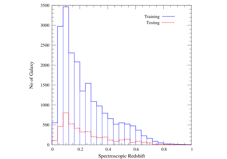
SDSS stripe 82 catalog has been used for the analysis of the present work (Annis et al., 2014). SDSS stripe 82 catalog has an area of 270 square degrees and is two magnitudes fainter than normal SDSS catalog. Galaxies have 5 bands photometry namely, , , , and . We take the entire ‘galaxy’ catalog and search for availability of spectroscopic redshift in SDSS. We find total 25120 galaxies having spectroscopic redshifts. Out of these, we construct the training set consisting of 20809 galaxies and a separate testing set of 4311 galaxies. The spectroscopic redshift distributions for both training data set and validation data set are shown in Fig. 1. Note that same data set is used to show results considering only 4 bands removing the band photometry. Further, we use our code on the entire stripe 82 catalog to find photometric redshift. In this case we use galaxies with that is 50% completeness limit of the stripe 82 catalog, along with cut off on the photometric uncertainty of in , and bands (Annis et al., 2014).
3 Clustering algorithm of sources
The clustering of data is a widely used statistical tool that has applications in various fields such as machine learning, optimisation, forecasting etc. Different clustering mechanism includes hierarchical clustering, density based, centroid based clustering etc., (Jain and Dubes, 1988). In the present work we divide the training set of data into several clusters before feeding it into the neural network. Most of the clustering techniques consider the true value of the data only and do not take account of the associated errors in the measurements (Chaudhuri and Bhowmik, 1998; Zhang and Zhao, 2004; Kumar and Patel, 2007; Ball and Brunner, 2010; Bhatnagar et al., 2012; Ishida and de Souza, 2013). In our clustering mechanism we modify the traditional methods in order to incorporate the errors in the data points. Further, we do not fix the number of clusters that we wish to make. Rather, given a criteria, we seek if a data point (in our case a galaxy) can form a cluster with other data points or not. If not, we consider that the data point as isolated. Below we describe our clustering mechanism in details.
A data point in the training set have input patterns (i.e. the photometric measurements in our case) and one desired output (in our case the spectroscopic redshift, ). Since the photometric redshift () depends more on the difference of fluxes in different bands rather than the flux in individual bands we only consider all possible combinations of flux differences as input patterns. This means for a galaxy with 5 bands photometric measurements we have differences; we denote them as , to . Each would have an error associated with them and we add the errors of the corresponding photometric bands in quadrature to determine error in and call it . Similarly, a cluster (say , the th cluster) also has input patterns, (the average of all cluster members), dispersions () associated with each pattern and one output pattern, the average redshift of the members of the cluster, . Thus a cluster can be described like a function where runs from (in our case) 1 to , if is the number of photometric bands for which measurements are available. Further, , and are calculated as follows. Consider that the cluster consists of members/galaxies. The weighted average of cluster properties, , are calculated as
| (1) |
Here we use the errors for each member as weights to calculate the mean and the index indicates the particular member. The dispersions in are obtained from
| (2) |
and the average redshift of the cluster is
| (3) |
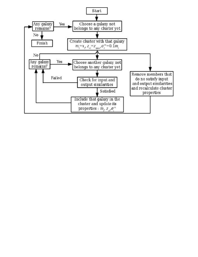
We start with a single galaxy that is not part of any cluster yet and consider it to be the first member of a cluster, . At this point, the cluster has , to and . Since the cluster has only one member, we assume . Now we search entire data base to find other members that have similar properties of the cluster. For each galaxy that has not been included in any existing clusters, we calculate the input similarity as
| (4) |
Note that we use both the errors in and dispersion of properties in cluster members to calculate the probability function . This number represents how much the galaxy differs from the cluster, in terms of input properties and actually is the log likelihood function excluding some constant terms. We can understand that if is less than , roughly, all including associated errors are within one sigma of the mean of the cluster. We say that the galaxy passes the input similarity test with that cluster if . Here, is some predefined number of order unity which governs the similarity test. Further, we calculate the output similarity between a galaxy and cluster as with is the average redshift of the cluster members and is the spectroscopic redshift of the galaxy in consideration. Note that we do not consider any error in this case as spectroscopic redshifts have very small errors. A galaxy is said to pass the output similarity test if , where is some predefined threshold value. If a galaxy passes both the input and output similarity tests, it is included in the cluster and we update the cluster properties using Eqs. 1-3.
We search the entire data set in this process to find all possible members of the cluster. Note that both and are dynamic properties of the cluster and are changing as each new member is added to the cluster. Hence it is possible that for some of the members the input and output similarity tests may result negative after all members of the cluster are identified. We check for such members and remove them from the cluster and recalculate the cluster properties. We do this iteration only once. When it is finished, we start again with some other galaxy that is not part of any existing clusters to form a new cluster. This process is repeated until all the galaxies have been considered to form a cluster. It may possible that a galaxy does not find any other galaxy to form cluster and we consider such galaxies as isolated ones. Moreover, the clusters with number of members less than 20 are not considered to take part in the neural network training as an individual cluster due to very small number statistics. Hence, we try to distribute those galaxies in existing clusters if they pass the input and output similarity tests. We check this when all the clusters are already been identified. The entire algorithm is shown by a flow chart in Fig. 2
Note that all galaxies in the training set do not necessarily be part of some cluster. Both and determine the number of clusters and the size and dispersion of the individual clusters as well as the number of galaxies that belong to all the clusters. For example, using and produce 251 clusters having more than 20 members and only 9330 galaxies out of 20809 galaxies form those clusters. On the other hand, making creates 262 clusters including total 12298 galaxies. We use these clusters to train separate neural networks.
4 Back propagation Neural Network
Artificial neural network has widely been used in different fields of machine learning (Gulati et al., 1994a, b, 1997; Mukherjee et al., 1996; Singh et al., 1998; Bazarghan and Gupta, 2008; Bora et al., 2009). Here we use neural network with back propagation learning to estimate photometric redshift from the fluxes at different bands. As the name suggests, the error in the output node propagates backward to update weights at different layers of network. This is also called supervised learning methods (see Bishop, 1995, for more details). The first layer of our network consists of nodes, the colors. Note that we rescale all values between 0 and in the first layer of nodes. This node is connected to an intermediate hidden layer of nodes where is equal to the closest integer of . We find this is the optimised number of nodes. Increasing this would not improved much but takes much more computational time, where as reducing would lead to poorer results. The first and hidden layers are connected by weight parameters where runs from 1 to and ranges from 1 to . The hidden layer is connected to output layer by weight parameters , to . We use as the activation function with is some parameter that governs the slope of the activation function. The advantage of taking this activation function is that it is nonlinear, continuous, differentiable and bounded between -1 to 1 and such functions provide excellent result in gradient base method (Mhaskar and Micchelli, 1994). We start with and gradually lower its value as the iteration increases. This ensures to reach much closer to the global minimum. In the feed-forward neural network method the output photometric redshifts are obtained from (Bishop, 1995),
| (5) |
| (6) |
The weights are updated using back propagation gradient descent method as,
| (7) | |||||
| (8) | |||||
| (9) |
Here and are the increments in the weights and is the learning parameter.
Note that we use separate networks for each clusters having member greater than 20 and another separate network for the entire galaxy sample. For clusters we use maximum 2000 iterations and for the whole sample it is 1,00,000 and take the best weight factors that minimize the error function, .
5 Photometric redshift using CuBAN
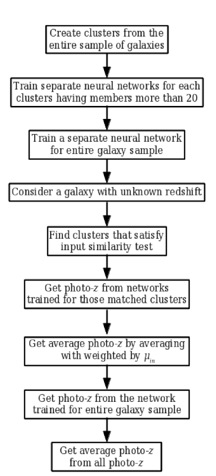
CuBAN is the name of our photometric redshift estimator. The name is derived from Clustering aided Back propagation Neural network photo- estimator. As the name suggests we use clustering of training sources (as already described in section 3) first and then use back propagation neural network (described in the previous section) to train the networks and use them to get photometric redshifts for unknown sources. For an unknown source we first look for clusters that satisfy the input similarity test i.e. , then use the networks trained for those clusters to estimate the photometric redshifts and corresponding errors. If a galaxy has more than one cluster satisfying the input similarity test, we use weighted average to estimate the redshift of that galaxy. The values of are used as the inverse of the weights. Note that a smaller value of implies a better match with the corresponding cluster and hence get more weighting in determining the average photometric redshift. Further, we use the network trained with the whole sample to estimate the redshift for galaxies that do not pass input similarity test with any training set clusters111We call sources that pass similarity tests as clustered sources and others as unclustered sources.. Since each cluster having members on average of between 50 to 100, we also provide a weighted average of redshift calculated using the clustered networks and the whole sample to remove any bias due to small number. We use the uncertainty in the redshift as the weights in this case. In Fig. 3 we show the block diagram that CuBAN follows.
The error in the estimate of the photometric redshift is a major concern and we deal with that quite rigorously here. From Eqn. 5 and 6, we can say that the photometric redshift derived using neural network is a function of , and , i.e.
| (10) |
Therefore, the error in can be thought of due to two parts, one due to errors in the i.e. in the flux measurements, and secondly uncertainty in the values of , that are obtained through the training. The error due to photometric uncertainty can be calculated by taking the derivative of the Eqn. 6 keeping as constants i.e.
| (11) | |||||
| (12) |
However, the error due to uncertainty in the weights can not be calculated in this way. Since there is no straight forward measure of the uncertainty of the weights we take the residual rms in the training set as a proxy for the total uncertainty in redshift due to uncertainty in all the weights combined. Then we add these two errors in quadrature to get the final uncertainty in the value of photometric redshift.
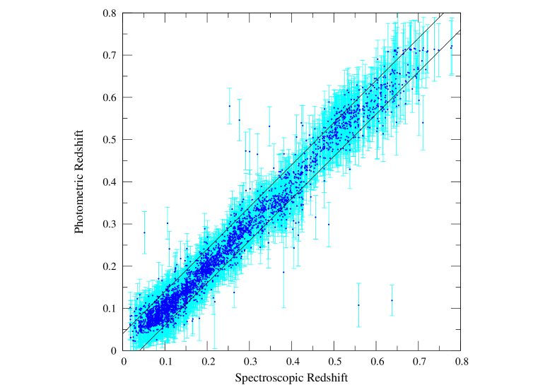
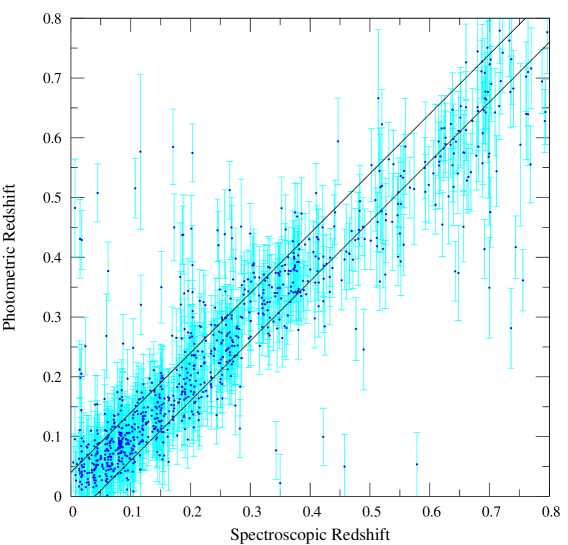
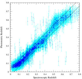
We now show our results using the code CuBAN on the SDSS stripe 82 catalog. Fig. 4 shows the prediction of photometric redshift by CuBAN against spectroscopic redshift for our 4213 test galaxies. Note that our training set consists of 20809 galaxies. Here we assume and . These criteria produce 262 clusters with more than 20 members. All these clusters contain a total of 12298 galaxies which is of total training set. For the clusters the rms errors (i.e. ) are of the order of few times and for the whole sample final rms error is 0.048 on the training set itself. For the test set consisting of 4312 galaxies, we find 3406 galaxies pass the input similarity test with one or more training set clusters and rest 906 galaxies do not pass similarity test with any cluster of the training set. For the 3406 clustered sources, the rms error is as low as 0.034 where as for the rest of the sample is 0.097 making a total of 0.054 for the entire sample. Note that in the training set there are very few galaxies with (around 300). Hence we should not consider anything beyond . If we restrict ourself with such criterion the rms error for the entire sample reduces to 0.045. In compare to the existing ANNz code the same set of training and testing set produces rms error of 0.055. We summarise our results in Table 1.
| Galaxy sample | No. of galaxies | rms error |
|---|---|---|
| Training set: All | 20809 | 0.048 |
| Testing set: Clustered | 3406 | 0.034 |
| Testing set: non-clustered | 906 | 0.097 |
| Testing set: All | 4312 | 0.054 |
| Testing set: | 4005 | 0.045 |
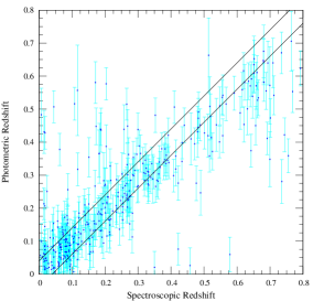
Hence, CuBAN provides very accurate redshift estimation from photometric measurements especially sources that match with existing clusters (i.e. pass the input similarity test) of the training set. This is clearly reflected in the top panel of Fig. 4 as well. In Fig. 4 we show photo- estimated from CuBAN against the spectroscopic redshift for both clustered (top panel) and unclustered (bottom) sources/galaxies in the testing set along with the estimated uncertainty. Only a handful of outliers is present there in the top panel. Most of the points along with the estimated errors lie well within the limits as shown by the two parallel lines222 parallel lines in Fig. 4 and in other figures corresponds to limits.. On the other hand the unclustered sources show little more scatter (bottom panel of Fig. 4) compare to the clustered sources. This is also reflected naturally on the estimated errors as we deal with them properly. The errors in the estimated photometric redshifts for the clustered sources are on average lower compared to the errors estimated for the rest of the sources.
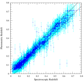
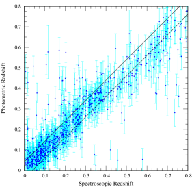
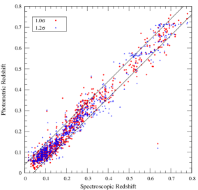
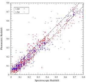
Thus the clustering is an important leap in predicting the photometric redshift. The properties of clusters depend on the two parameters, and . In Fig. 5 we show the effect of cluster properties on the estimated redshifts. In the top panel we change . This leads to form 251 clusters with 9330 galaxies (only 45% of total sample). In case of the testing set, only 2684 sources pass the input similarity test with training set clusters. In this case the rms errors for the clustered and unclustered sources are 0.034 and 0.077 respectively making total rms 0.54. Thus it does not make any comprehensible difference in predicted photo-. The rms for unclustered sources is reduced as the number of unclustered sources has increased but CuBAN is still predicting very good redshift for them using the network trained by the entire galaxy sample. The difference between and 1.2 is shown in top right panel of Fig. 5 where we show the photometric redshift estimated for the sources that belongs to some cluster when but do not fall in any cluster when . These are the sources for which the photo- are calculated in two different methods; when photo-s are obtained from the network that was trained using the entire galaxy sample where as in other case the photo-s are obtained using networks for the clustered sources. It is clear from the figure that there is not much difference in this case. However, assuming shows prominent effect. With this assumption, more sources become part of clusters, in case of training set and 3938 for the testing set. Again, the difference is clear in the bottom right panel of Fig. 5 where the scatter in predicted photometric redshifts from the two different networks (cluster networks and whole sample network) is obvious. In this case the clustering is producing clusters having member with a larger dispersion in photometric properties as we have relaxed the criteria of being part of a cluster and that is reflected in the predicted photometric redshifts. Thus we find provides optimised results for this data set, and we use it to do the further analysis of getting photometric redshift for the entire stripe 82 catalog.
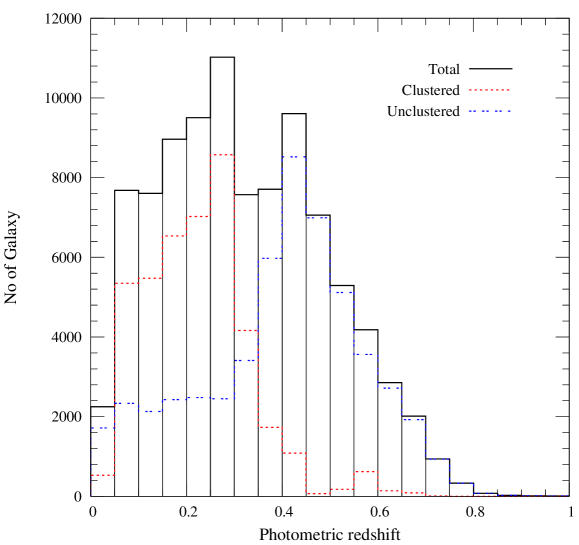
In Fig. 6 we show the distribution of photo- for the half of the stripe 82 catalog consisting of 94718 galaxies. Note that we do not put any flux cut off for these sample (see section 2). As expected the redshift distribution shows a peak at as the effective survey volume increases with increasing redshift. However, after that the number of sources decreases due to decreasing flux of the sources for larger distance. Hence CuBAN is providing a good estimation of the redshift. Further, it is also obvious from the figure that the sources that pass the similarity test decrease rapidly at higher redshift as the number of training sources/clusters decreases.
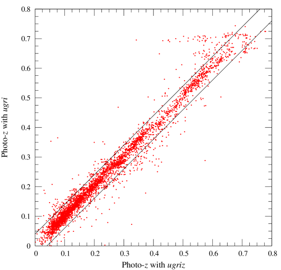
Finally, we show that CuBAN provides reasonable results even if we have measurements for lesser number of photometric bands. This is resulted from the use of colors rather than the individual fluxes in training the neural networks. Fig. 7 compares the photometric redshift estimated for 5 bands and 4 bands photometry of the same data. No obvious mismatch is observed except perhaps at where we have very small number of galaxies in training set itself. Further, CuBAN also provides better results even if there are less number of data for training. We randomly choose 2000 galaxies to form a new training set. With this set the rms for 4312 test set galaxies in CuBAN is 0.06 where as ANNz provides rms error of 0.10.
6 User Manual of CuBAN
CuBAN is freely available from https://goo.gl/fpk90V or https://sites.google.com/site/sscubanz/ under gnu public license agreement. We provide entire source code written in C which is very easy to compile, run and even modify. It can be run on any machine having standard C compiler. In the package, we provide a header file, cnn.h, a text file containing the names of catalog files, file_names.txt, the source code, cubanz.c and a README file for general instructions. In the cnn.h file there are two lines as
#define no_of_galaxy 20809
#define no_of_bands 5
no_of_galaxy is the number of sources available for the training with
spectroscopic redshift and no_of_bands is the number of photometric
bands data that the training set has. One needs to modify these values according
to the requirement. The catalog names and output file names
are to be mentioned in the file_names.txt file in the following order:
1. Name of file containing the training set
2. Name of file containing the test data set
3. File name where output for test data would be written
4. File name of catalog for which you wish to get photo-
5. File name where output for given catalog (4) would be written.
The training and testing catalog should have all photometric measurements first
and then their corresponding errors. The first columns should have
the apparent magnitudes of photometric bands and next columns
should contain the corresponding errors in magnitude. The last column should have the
spectroscopic redshift. The catalog for which one wishes to get the photo-
should have the data in same order except the redshift information of course.
The source code can be compile with any standard C compiler say, cc, as cc cubanz.c -lm -o cubanz.o. This will produce the executable cubanz.o. Running the executable will give the desire photo-. The output file for the test data would contain the following columns: (1) serial number, (2) spectroscopic redshift, (3) photometric redshift from clusters (if the source does not pass input similarity test with any training cluster it would be -10), (4) error in column 3, (5) value of best (for unclustered source it is 100), (6) cluster tag (1 for clustered source, -1 otherwise), (7) number of clusters that pass input similarity test with the source, (8) photometric redshift using neural network with whole sample, (9) error in column 8, (10) weighted average photo- from column 3 and column 8, (11) error in column 10. The output for the actual catalog with unknown redshift will have all the columns except spectroscopic redshift of course. Note that it will also produce a log file with name cnn_out.log that contains every details of what the code is doing.
7 Discussions and Conclusions
We have introduced a new photometric redshift estimator, CuBAN, that provides a much better photo- compared to the existing ones. The code is publicly available and very simple to use. It can be run in any machine having standard C compiler. It uses back propagation neural networks clubbed with clustering of training sources with known photometric broad band fluxes and spectroscopic redshifts. The clustering technique enables us to get a better estimate of photometric redshifts particularly for galaxies that fall under clusters. In particular the rms residue in the testing set is as low as 0.03 for a wide redshift range of compare to existing ANNz code that gives 0.055 on the same data set. Moreover, we provide much better estimate on the uncertainty in the redshift estimator considering the uncertainty in the weight factors of the trained neural networks. We hope that it will be very useful to the astronomy community given the existing large photometric data as well as large upcoming photometric surveys. The present version of the code is very simple and we are in the process of making it more flexible as well as user friendly.
Acknowlegdements
SSP thanks Department of Science and Technology (DST), India for the INSPIRE fellowship. We thank an anonymous referee for useful comments that have helped in improving our paper.
References
- Abdalla et al. (2011) Abdalla, F. B., Banerji, M., Lahav, O., Rashkov, V., Nov. 2011. A comparison of six photometric redshift methods applied to 1.5 million luminous red galaxies. MNRAS 417, 1891–1903.
- Ahn et al. (2014) Ahn, C. P., Alexandroff, R., Allende Prieto, C., Anders, F., Anderson, S. F., Anderton, T., Andrews, B. H., Aubourg, É., Bailey, S., Bastien, F. A., et al., Apr. 2014. The Tenth Data Release of the Sloan Digital Sky Survey: First Spectroscopic Data from the SDSS-III Apache Point Observatory Galactic Evolution Experiment. ApJS 211, 17.
- Annis et al. (2014) Annis, J., Soares-Santos, M., Strauss, M. A., Becker, A. C., Dodelson, S., Fan, X., Gunn, J. E., Hao, J., Ivezić, Ž., Jester, S., Jiang, L., Johnston, D. E., Kubo, J. M., Lampeitl, H., Lin, H., Lupton, R. H., Miknaitis, G., Seo, H.-J., Simet, M., Yanny, B., Oct. 2014. The Sloan Digital Sky Survey Coadd: 275 deg2 of Deep Sloan Digital Sky Survey Imaging on Stripe 82. ApJ 794, 120.
- Babbedge et al. (2004) Babbedge, T. S. R., Rowan-Robinson, M., Gonzalez-Solares, E., Polletta, M., Berta, S., Pérez-Fournon, I., Oliver, S., Salaman, D. M., Irwin, M., Weatherley, S. J., Sep. 2004. IMPZ: a new photometric redshift code for galaxies and quasars. MNRAS 353, 654–672.
- Ball and Brunner (2010) Ball, N. M., Brunner, R. J., 2010. Data Mining and Machine Learning in Astronomy. International Journal of Modern Physics D 19, 1049–1106.
- Bazarghan and Gupta (2008) Bazarghan, M., Gupta, R., Jun. 2008. Automated classification of sloan digital sky survey (SDSS) stellar spectra using artificial neural networks. Ap&SS 315, 201–210.
- Benítez (2000) Benítez, N., Jun. 2000. Bayesian Photometric Redshift Estimation. ApJ 536, 571–583.
- Bhatnagar et al. (2012) Bhatnagar, V., Dobariyal, R., Jain, P., Mahabal, A., Oct. 2012. Data Understanding using Semi-Supervised Clustering. Conference on Intelligent Data Understanding (CIDU), 2012, 118–123.
- Bishop (1995) Bishop, C., 1995. Neural Networks for Pattern Recognition. Advanced Texts in Econometrics. Clarendon Press.
- Bleem et al. (2015) Bleem, L. E., Stalder, B., Brodwin, M., Busha, M. T., Gladders, M. D., High, F. W., Rest, A., Wechsler, R. H., Jan. 2015. A New Reduction of the Blanco Cosmology Survey: An Optically Selected Galaxy Cluster Catalog and a Public Release of Optical Data Products. ApJS 216, 20.
- Bolzonella et al. (2000) Bolzonella, M., Miralles, J.-M., Pelló, R., Nov. 2000. Photometric redshifts based on standard SED fitting procedures. A&A 363, 476–492.
- Bonfield et al. (2010) Bonfield, D. G., Sun, Y., Davey, N., Jarvis, M. J., Abdalla, F. B., Banerji, M., Adams, R. G., Jun. 2010. Photometric redshift estimation using Gaussian processes. MNRAS 405, 987–994.
- Bora et al. (2009) Bora, A., Gupta, R., Singh, H. P., Duorah, K., Nov. 2009. Automated star-galaxy segregation using spectral and integrated band data for TAUVEX/ASTROSAT satellite data pipeline. New A 14, 649–653.
- Chaudhuri and Bhowmik (1998) Chaudhuri, B., Bhowmik, P., 1998. An approach of clustering data with noisy or imprecise feature measurement. Pattern Recognition Letters 19 (14), 1307 – 1317.
- Colless (1999) Colless, M., Jan. 1999. First results from the 2dF Galaxy Redshift Survey. Philosophical Transactions of the Royal Society of London Series A 357, 105.
- Collister and Lahav (2004) Collister, A. A., Lahav, O., Apr. 2004. ANNz: Estimating Photometric Redshifts Using Artificial Neural Networks. PASP 116, 345–351.
- Feldmann et al. (2006) Feldmann, R., Carollo, C. M., Porciani, C., Lilly, S. J., Capak, P., Taniguchi, Y., Le Fèvre, O., Renzini, A., Scoville, N., Ajiki, M., Aussel, H., Contini, T., McCracken, H., Mobasher, B., Murayama, T., Sanders, D., Sasaki, S., Scarlata, C., Scodeggio, M., Shioya, Y., Silverman, J., Takahashi, M., Thompson, D., Zamorani, G., Oct. 2006. The Zurich Extragalactic Bayesian Redshift Analyzer and its first application: COSMOS. MNRAS 372, 565–577.
- Gerdes et al. (2010) Gerdes, D. W., Sypniewski, A. J., McKay, T. A., Hao, J., Weis, M. R., Wechsler, R. H., Busha, M. T., Jun. 2010. ArborZ: Photometric Redshifts Using Boosted Decision Trees. ApJ 715, 823–832.
- Gulati et al. (1994a) Gulati, R. K., Gupta, R., Gothoskar, P., Khobragade, S., May 1994a. Stellar spectral classification using automated schemes. ApJ 426, 340–344.
- Gulati et al. (1994b) Gulati, R. K., Gupta, R., Gothoskar, P., Khobragade, S., 1994b. Ultraviolet stellar spectral classification using a multilevel tree neural network. Vistas in Astronomy 38, 293–298.
- Gulati et al. (1997) Gulati, R. K., Gupta, R., Rao, N. K., Jun. 1997. A comparison of synthetic and observed spectra for G-K dwarfs using artificial neural networks. A&A 322, 933–937.
- Hogan et al. (2015) Hogan, R., Fairbairn, M., Seeburn, N., May 2015. GAz: a genetic algorithm for photometric redshift estimation. MNRAS 449, 2040–2046.
- Ishida and de Souza (2013) Ishida, E. E. O., de Souza, R. S., Mar. 2013. Kernel PCA for Type Ia supernovae photometric classification. MNRAS 430, 509–532.
- Ivezic et al. (2008) Ivezic, Z. et al. for the LSST Collaboration, May 2008. LSST: from Science Drivers to Reference Design and Anticipated Data Products. ArXiv e-prints.
- Jain and Dubes (1988) Jain, A., Dubes, R., 1988. Algorithms for clustering data. Prentice-Hall Advanced Reference Series. Prentice Hall PTR.
- Kumar and Patel (2007) Kumar, M., Patel, N. R., 2007. Clustering data with measurement errors. Computational Statistics & Data Analysis 51 (12), 6084 – 6101.
- Lecun et al. (1998) Lecun, Y., Bottou, L., Orr, G. B., Müller, K.-R., 1998. Efficient backprop.
- Mhaskar and Micchelli (1994) Mhaskar, H. N., Micchelli, C. A., 1994. How to choose an activation function. In: Cowan, J. D., Tesauro, G., Alspector, J. (Eds.), Advances in Neural Information Processing Systems 6. Morgan-Kaufmann, pp. 319–326.
- Mukherjee et al. (1996) Mukherjee, S., Bhattacharya, U., Parui, S. K., Gupta, R., Gulati, R. K., Sep. 1996. A multi-layered backpropagation artificial neural network algorithm for UV spectral classification. Ap&SS 239, 361–373.
- Singh et al. (1998) Singh, H. P., Gulati, R. K., Gupta, R., Apr. 1998. Stellar Spectral Classification using Principal Component Analysis and Artificial Neural Networks. MNRAS 295, 312–318.
- Zhang and Zhao (2004) Zhang, Y., Zhao, Y., Aug. 2004. Automated clustering algorithms for classification of astronomical objects. A&A 422, 1113–1121.