Convolution kernels for multi-wavelength imaging

Astrophysical images issued from different instruments and/or spectral bands often require to be processed together, either for fitting or comparison purposes. However each image is affected by an instrumental response, also known as PSF, that depends on the characteristics of the instrument as well as the wavelength and the observing strategy. Given the knowledge of the PSF in each band, a straightforward way of processing images is to homogenise them all to a target PSF using convolution kernels, so that they appear as if they had been acquired by the same instrument. We propose an algorithm that generates such PSF-matching kernels, based on Wiener filtering with a tunable regularisation parameter. This method ensures all anisotropic features in the PSFs to be taken into account. We compare our method to existing procedures using measured Herschel/PACS and SPIRE PSFs and simulated JWST/MIRI PSFs. Significant gains up to two orders of magnitude are obtained with respect to the use of kernels computed assuming Gaussian or circularised PSFs. A software to compute these kernels is available at https://github.com/aboucaud/pypher.

1 Introduction

The point-spread function (PSF), also known as beam, is one of the main characteristics of any astronomical imager. It is a model of the diffraction pattern resulting from the interaction between the electromagnetic radiation and the instrument optics and detectors at every wavelength. Since most instruments operate on a single or a series of bandpasses (through e.g. filters), the resulting effective PSF is an integral of the monochromatic PSFs over the wavelength range, weighted by the instrumental throughput and the source energy distribution of a given astronomical object. A more accurate model can even include convolutional effects such as guiding errors, trailing effects from a scanning mode, smearing by the detector response or even non-convolutional effects like the brighter-fatter effect. Once imaged, these model PSFs exhibit a complex shape, including anisotropy, wings and spikes that extend far from the center. Another classic feature of the PSF derived from the laws of optics is the radially oscillating pattern of the response, (especially in the monochromatic case) creating a series of peaks and valleys. These secondary peaks can account for a non negligible amount of the total power of the PSF. For ground-based astronomy though, the atmospheric turbulence creates a smearing that redistributes the power of these peaks and valleys and enables the PSF to be modeled by simple analytic profiles like 2D Gaussians. On the contrary, space telescopes can benefit from a much higher resolution at the expense of a full complexity of the PSF. To cite a few examples, the effective PSF of IRAS maps was elliptical due to the scanning strategy, so the angular resolution was strongly anisotropic, with ratios up to 1:6 (e.g. 0.75’ $\times$ 4.6’ at 25 $\mu$m, from Wheelock et al., 1994). More recently, the effective PSFs of the Planck/HFI maps appeared to have an ellipticity in a range 1.04 to 1.4, depending on the spectral band (Ade et al., 2011), and the PSF of the PACS photometer (Poglitsch et al., 2010) onboard the Herschel satellite, characterised by Lutz (2012), showed a narrow core, a tri-lobe pattern and Knotty structured diffraction rings. As we push both optical performances and detector capabilities of the future missions towards the boundaries, the optical design highly increases in complexity. Hence, for upcoming space surveys (Euclid, WFIRST) or observatories (Athena or JWST), the characterisation and processing of elaborated PSFs become a crucial task.

Most of astrophysical studies necessitate multi-wavelength observations, either from multiple bands/filters within an instrument or from various instruments and telescopes. The different maps are affected by a particular PSF and the pixel-based data comparison cannot be straightforward. However, a technique widely used in multi-band photometry is to perform the measurements on PSF homogenised data, that is to select a dataset as reference (usually the one with the worst resolution, or wider PSF) and transform the other datasets so they are PSF-matched with the reference PSF, a technique called PSF homogenisation or PSF matching (see e.g. Bertin et al., 2002; Gordon et al., 2008; Darnell et al., 2009; Hildebrandt et al., 2012). PSF homogenisation is usually achieved by convolving the image with a kernel that is generated from the PSF corresponding to the image and the reference PSF. In the literature, one can distinguish between parametric kernels which use a fit of an analytic model to each PSF (Moffat, multiple Gaussians, etc.) or their decomposition on a proper basis (e.g. Gauss-Hermite polynomials, or shapelets), and results in an analytic expression for the kernel (e.g. Kuijken, 2008; Hildebrandt et al., 2012) ; and non parametric methods that use pixel information from the image (e.g. Alard, 2000) or adopt effective PSF images (e.g. Gordon et al., 2008; Aniano et al., 2011) to compute the kernels.

With the purpose of taking into account the full complexity and angular extension of space instruments’ PSFs, we address the creation of PSF-matching kernels for multi-wavelength studies. We then present two usecases for these kernels, one based on the Herschel satellite data, and a second on simulations for the MIRI instrument of JWST. We also deliver a program called pypher that computes the kernels given two PSF images (see Appendix A). This code has initially been developed in preparation for the Euclid mission (Laureijs et al., 2010).

In Section 2, we describe the algorithm for the generation of convolution kernels used to match the resolution of images. In Section 3, we assess the improvement brought by these kernels on the multi-wavelength study of dust properties with the Herschel satellite, and show in Section 4 the reconstruction power of such kernels on PSF simulations of the future JWST satellite, before summarising this work in Section 5.

2 Kernel generation

2.1 Data Model

Let’s first consider an astrophysical image $\boldsymbol{y}$, observed with an instrument modeled as a linear invariant system:

$$\boldsymbol{y}=\boldsymbol{h}\ast\boldsymbol{x}+\boldsymbol{n}\,,$$ (1)

where $\boldsymbol{h}$ is the PSF convolved with the unknown sky $\boldsymbol{x}$, $\boldsymbol{n}$ is the image noise and $\ast$ stands for the discrete convolution (see e.g. Gonzalez & Woods, 2008).

Given two PSF models $\boldsymbol{h}_{a}$ and $\boldsymbol{h}_{b}$, where $a$ and $b$ refer to different frequency bands from the same or various instruments, the process we are interested in, referred to as PSF-matching, is to transform the image $\boldsymbol{y}_{a}$ acquired at the angular resolution of $\boldsymbol{h}_{a}$

$$\boldsymbol{y}_{a}=\boldsymbol{h}_{a}\ast\boldsymbol{x}+\boldsymbol{n}_{a}\,,$$ (2)

into an image $\boldsymbol{y}_{a,b}$ at the angular resolution of $\boldsymbol{h}_{b}$

$$\boldsymbol{y}_{a,b} =\boldsymbol{k}_{a,b}\ast\boldsymbol{y}_{a}\,,$$ (3)

$$\simeq\boldsymbol{h}_{b}\ast\boldsymbol{x}$$ (4)

where $\boldsymbol{k}_{a,b}$ is the matching kernel from $\boldsymbol{h}_{a}$ to $\boldsymbol{h}_{b}$.

This paper presents a linear algorithm that computes the kernel $\boldsymbol{k}_{a,b}$ to produce the image $\boldsymbol{y}_{a,b}$ from the original image $\boldsymbol{y}_{a}$ through a convolution. To this end, we need to construct the kernel $\boldsymbol{k}_{a,b}$ such that

$$\boldsymbol{h}_{b}=\boldsymbol{h}_{a}\ast\boldsymbol{k}_{a,b}\,.$$ (5)

2.2 Kernel generation

For such linear systems as equation (5), one can seek an estimate of $\boldsymbol{k}_{a,b}$, denoted $\hat{\boldsymbol{k}}_{a,b}$, that minimises the least squares criterion $J$

$$\hat{\boldsymbol{k}}_{a,b} =\mathop{\mathrm{arg\,min}}_{\boldsymbol{k}_{a,b}}J(\boldsymbol{k}_{a,b})\,,$$ (6)

$$=\mathop{\mathrm{arg\,min}}_{\boldsymbol{k}_{a,b}}\left\|\boldsymbol{h}_{b}-\boldsymbol{h}_{a}\ast\boldsymbol{k}_{a,b}\right\|^{2}\,.$$ (7)

However, the presence of the convolution makes the system ill-posed for the inversion, hence the solution to equation (7) is not stable. The only way to stabilise the solution is to add information. For the considered system, we use a technique called regularisation. We choose a $\ell_{2}$ norm in order to have a linear estimator and use Fourier filtering, and penalise the high frequencies where we expect the noise to dominate, using a high-pass filter $\boldsymbol{d}$. This corresponds to adding a relative degree of smoothness between values of neighboring pixels.

$$J(\boldsymbol{k}_{a,b})=\left\|\boldsymbol{h}_{b}-\boldsymbol{h}_{a}\ast\boldsymbol{k}_{a,b}\right\|^{2}+\mu\left\|\boldsymbol{d}\ast\boldsymbol{k}_{a,b}\right\|^{2}\,,$$ (8)

where $\boldsymbol{d}$ is the second-order differential operator (i.e. two-dimensional Laplacian matrix)

$$\boldsymbol{d}=\begin{bmatrix}\leavevmode\nobreak\ 0&-1&\leavevmode\nobreak\ 0\\ -1&\leavevmode\nobreak\ 4&-1\\ \leavevmode\nobreak\ 0&-1&\leavevmode\nobreak\ 0\end{bmatrix}$$ (9)

and $\mu$ the regularisation parameter, which tunes the balance between the data fidelity and the penalisation. Other norms, such as $\ell_{1}$, $\ell_{2}\ell_{1}$ or $TV$ (Total Variations) are known to better preserve the image details, but produce non linear estimators that require iterative algorithms to solve.

Denoting the Fourier transform of any two-dimensional vector $\boldsymbol{u}$ by $\tilde{\boldsymbol{u}}$, the convolution theorem states that the real space convolution is equivalent to a termwise product in Fourier space

$$\boldsymbol{h}\ast\boldsymbol{k}\Leftrightarrow\tilde{\boldsymbol{h}}\odot\tilde{\boldsymbol{k}}\,,$$ (10)

where $\odot$ symbolises the termwise product between vectors/matrices.

Under these assumptions, the cancellation of the first gradient of the criterion (8) leads to the classical regularised mean square solution of equation (7) in Fourier space

$$\tilde{\hat{\boldsymbol{k}}}_{a,b}=\boldsymbol{w}\odot\tilde{\boldsymbol{h}}_{b}$$ (11)

where $\boldsymbol{w}$ is a Wiener filter with high-frequency penalisation

$$\boldsymbol{w}(\mu)=\frac{\tilde{\boldsymbol{h}}_{a}^{{\dagger}}}{|\tilde{\boldsymbol{h}}_{a}|^{2}+\mu|\tilde{\boldsymbol{d}}|^{2}}\quad;\quad\mu\neq 0$$ (12)

and $\boldsymbol{\tilde{\boldsymbol{h}}_{a}}^{{\dagger}}$ stands for the complex conjugate of matrix $\boldsymbol{\tilde{\boldsymbol{h}}_{a}}$.

The real-space convolution kernel $\boldsymbol{k}_{a,b}$, is eventually obtained via the inverse Fourier transform of equation (11). For two instruments $a$ and $b$, this kernel is thus only parametrised by the regularisation parameter $\mu$. The optimal balance between the data and the penalisation is found by setting $\mu$ to the inverse of the signal-to-noise ratio (SNR) of the homogenised image, $\boldsymbol{y}_{a}$ in this case.

We provide with this paper the pypher program (see Appendix A), an implementation of the Algorithm 1 presented below, that computes $\boldsymbol{k}_{a,b}$.

inputs : $\boldsymbol{h}_{a}$ 2D array of size N_a $\times$ N_a and pixel scale p_a,
$\boldsymbol{h}_{b}$ 2D array of size N_b $\times$ N_b and pixel scale p_b,
angles $\alpha_{a}$ and $\alpha_{b}$ (see Appendix A)
regularisation factor $\mu$.

output : $\boldsymbol{k}_{a,b}$ 2D array of size N $\times$ N and pixel scale p.

  /* PSF warping: */

N = N_b ; p = p_b

for $i$ in {$a$, $b$} do

      if $\alpha_{i}\neq 0$ then

           rotate $\boldsymbol{h}_{i}$ through an angle $\alpha_{i}$

          

           end if

          

           end for

          if p${}_{a}\neq$ p then

                rescale $\boldsymbol{h}_{a}$ to the pixel scale p

               

                end if

               for $\boldsymbol{u}$ in {$\boldsymbol{h}_{a}$, $\boldsymbol{d}$} do

                     if size($\boldsymbol{u}$) ¡ N $\times$ N then

                          pad $\boldsymbol{u}$ with zeros to a size of N $\times$ N

                         

                          else

                               trim $\boldsymbol{u}$ to a size of N $\times$ N

                              

                               end if

                              

                               end for

                              

                                /* Wiener filter: */

                               for $\boldsymbol{u}$ in {$\boldsymbol{h}_{a}$, $\boldsymbol{d}$} do

                                    compute the OTF of $\boldsymbol{u}$: $\tilde{\boldsymbol{u}}$

                                   

                                    end for

                                   

                                   compute $\boldsymbol{w}(\mu)$ following equation (12)

                                   

                                     /* Kernel: */

                                    compute the discrete Fourier transform of $\boldsymbol{h}_{b}$: $\tilde{\boldsymbol{h}}_{b}$

                                    compute $\tilde{\hat{\boldsymbol{k}}}_{a,b}$ following equation (11) via a termwise product

                                    inverse Fourier transform $\tilde{\hat{\boldsymbol{k}}}_{a,b}$ to obtain the kernel $\boldsymbol{k}_{a,b}$

                                   

Algorithm 1 Matching kernel generation recipe

3 Impact on Herschel data analysis

The pypher kernels allow us to convolve multiple astronomical images to a common angular resolution. In order to preserve all the information during this process, a good knowledge of the effective PSFs of the instruments used is required. We focus here on the particular analysis of Herschel photometric images which have been widely used in the last few years to measure the dust temperature and the spectral index $\beta$ across many astronomical objects from multi-band imaging with PACS and SPIRE.

Given the uncertainties on the PSFs of PACS and SPIRE instruments, since the beginning of the operational period of Herschel and for a few years, convolutions from PACS to SPIRE angular resolution have been performed assuming Gaussian PSFs with a given FWHM estimated from dedicated observations of asteroids. In 2011, a better characterisation of the instruments’ PSFs allowed Aniano et al. (2011, ADGS11) to develop a method to construct convolution kernels assuming circular PSFs. While a full analysis of the PSF of the SPIRE instrument has been finalised recently by the Instrument Control Centre (ICC, Schultz, 2015), a final PSF characterisation for the PACS instrument has not been released yet by the ICC (Lutz, 2015). Parallel work has been performed by Bocchio et al. (2016), who have computed PACS effective PSFs from the combination of Vesta and Mars dedicated observations, which will be used hereafter. The current knowledge of both PACS and SPIRE PSFs, and the pypher code allow us to construct effective convolution kernels with an unprecedented precision. In this section we show how and to what extent the use of different convolution kernels can affect the results.

3.1 Herschel PSFs and kernels

For each Herschel band, $\lambda$, we define four PSF images:

1. the effective PSF ($E_{\lambda}$), taken from Bocchio et al. (2016) for PACS and Schultz (2015) for SPIRE ;

2. the Gaussian PSF ($G_{\lambda}$), computed fitting a 2D Gaussian profile to $E_{\lambda}$. $G_{\lambda}$ has the same FWHM as $E_{\lambda}$ but does not account for secondary lobes and faint structures ;

3. the circular PSF ($C_{\lambda}$), computed from $E_{\lambda}$ by averaging the image intensity in annular bins. All information on the asymmetry of the PSF is then lost ;

4. the Aniano PSF ($A_{\lambda}$), a circular PSF from the ADGS11 paper.

For each of the first three types of PSF, we define the corresponding matching kernels between the bands $\lambda_{1}$and $\lambda_{2}$ as

$$K^{X}_{\lambda_{1},\lambda_{2}}\quad\text{with}\quad X\in\{E,G,C\}$$ (13)

and compute them with pypher. We also consider the Aniano kernels defined here as $K^{A}_{\lambda_{1},\lambda_{2}}$ and computed in ADGS11 via a different method than that used in this work.

The homogenised images can therefore be denoted by

$$X_{70,350}=E_{70}\ast K_{70,350}^{X}\,.$$ (14)

Figure 1: Effective PACS 70 $\mu$m and SPIRE 350 $\mu$m PSFs on the left. The central column shows Gaussian, circular and effective kernels for these PSFs computed following the procedure described in Section 3.1. The corresponding relative residual images (see equation 15) are displayed in the right column. The bottom kernel and residual image correspond to this work. All images are $120^{\prime\prime}\times 120^{\prime\prime}$.

3.2 Kernel comparison

In this paragraph we assess the impact of using approximations of effective PSFs in the homogenisation process, which is directly related to the creation of the convolution kernel. The effective kernel $K^{E}_{\lambda_{1},\lambda_{2}}$ being the target of our kernel generation algorithm, it is expected to produce better results than the other types described above.

To compare the different types of kernels, we chose to measure the difference between the effective PSF at $\lambda_{1}$ matched to $\lambda_{2}$ and the effective PSF at $\lambda_{2}$. We define the relative residuals $R^{X}$ as

$$R^{X}_{\lambda_{1},\lambda_{2}}=\frac{|E_{\lambda_{2}}-E_{\lambda_{1}}\ast K^{X}_{\lambda_{1},\lambda_{2}}|}{E_{\lambda_{2}}}.$$ (15)

for each type of kernel.

For this comparison test, we consider the matching of the PACS 70 $\mu$m PSF to the resolution of SPIRE 350 $\mu$m. In the remainder of this paragraph, we refer to these bands as 70 and 350.

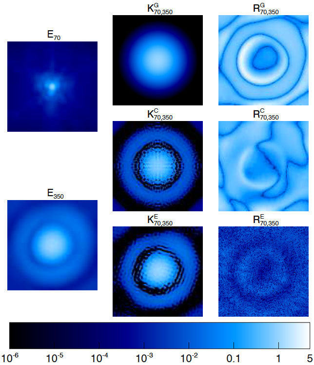
The two images on the left of Figure 1 represent the effective PSFs of PACS 70 $\mu$m: $E_{70}$ and SPIRE 350 $\mu$m: $E_{350}$. The central column shows the kernels computed with pypher from Gaussian (top) and circular (middle) approximations of the effective PSFs, as described in Section 3.1, and directly from the left-side PSFs (bottom). On these kernel images, one can see the characteristics of the input PSFs: the Gaussian approximation has a single lobe, the circular one is axisymmetrical and presents a second lobe, and the last one has two lobes and the general shape of $E_{350}$. Next to these kernels, the associated homogenisation residual images are displayed (see equation 15 for computation).

Figure 2: First ($m(r)$, top panel) and second ($\sigma(r)$, bottom panel) polar moments of the residuals (right column images of Figure 1 + $R^{A}_{70,350}$) as a function of the distance $r$ to the image center. The different lines represent the kernel types used for the homogenisation: Gaussian (red dotted), circular (green long dashed), ADGS11 (black dashed) and effective (blue solid, this work). The vertical black dotted line indicates the HWHM of the SPIRE 350 $\mu$m PSF.

Both $R^{G}_{70,350}$ and $R^{C}_{70,350}$ have residuals on the order of 10% within the first lobe of $E_{350}$ (central region of radius equal to the HWHM $\simeq 12^{\prime\prime}$). Outside of that region, the reconstruction from these two kernels is even worse. In particular, the extinction ring that marks the transition between the first and second lobe does not exist in the Gaussian case and is slightly shifted due to azimuthal averaging in the circular case, which leads to a big residual error in both cases (white circle on $R^{G}_{70,350}$ and $R^{C}_{70,350}$). Both kernel and residual images from ADGS11, which are not shown on Figure 1, present very similar behaviour to the circular approximation. Using the kernel constructed with effective PSFs, $R^{E}_{70,350}$, we obtain very homogeneous residuals of the order of 0.1%.

To analyse in more details these residuals, we introduce the first $m$ and second $\sigma$ polar moments of the residuals:

$$m(r) =\frac{1}{n_{\rm ang}}\sum_{i=1}^{n_{\rm ang}}R^{X}(r,\theta_{i}),$$

$$\sigma(r) =\sqrt{\frac{1}{n_{\rm ang}}\sum_{i=1}^{n_{\rm ang}}\left[R^{X}(r,\theta_{i})\right]^{2}}\,,$$ (16)

where $R^{X}(r,\theta_{i})$ is the intensity of the residual image (computed using the kernel $X$) at a distance $r$ from the image centre and at an angle $\theta_{i}=2\pi i/n_{\rm ang}$, with $n_{\rm ang}=100$. The moments express the intensity and dispersion of the residuals along the PSF radius.

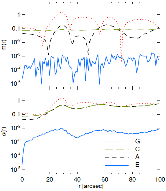
Figure 2 shows these two values computed on the residual images for the four kernel types. As previously stated, the Gaussian case (dotted red lines) is only stable within a circle of radius equal to the HWHM of $E_{350}$. At further distance it shows very high first and second moments, close to unity, and establishes a very poor matching. The circular case (long-dashed green) exhibits a constant first moment below 10% at all distances, better than the Gaussian case. This is mainly due to the computation of the first moment that is very similar to the circularising process and averages out the measurements. However, the asymmetry and local structures of $E_{70}$ and $E_{350}$ are lost and the second moment is comparable to that of $R^{G}_{70,350}$. ADGS11 used narrower versions of PACS and SPIRE PSFs than those used in this work to produce the kernels. Both first and second moments (dashed black) therefore present bumps at the position of the lobes. Finally, the effective case (blue) best matches $E_{350}$. In amplitude, the first moment is $\lesssim 0.1\%$ and the second moment $\lesssim 1\%$ at all distances, even if we note that the second moment presents the two bumps observed earlier. By comparison, these moments are two orders of magnitude lower than that of the other three cases.

This concludes in a major improvement in using pypher kernels with effective PSFs with respect to Gaussian, circular or ADGS11 kernels from an image processing standpoint. Next we test again these kernels on the determination of meaningful parameters from data or simulations.

3.3 Dust properties study

Herschel observations are often used to retrieve information on dust properties in our Galaxy as well as in local galaxies. In this section we show how the choice of PSFs to construct the convolution kernels can affect pixel-by-pixel measurements.

We consider an edge-on galaxy at $D\sim 10$ Mpc from us with an intrinsic vertical profile given by:

$$I_{\rm d}(z)=I_{\rm d}(0)\exp\left(\frac{-z}{z_{\rm d}}\right),$$ (17)

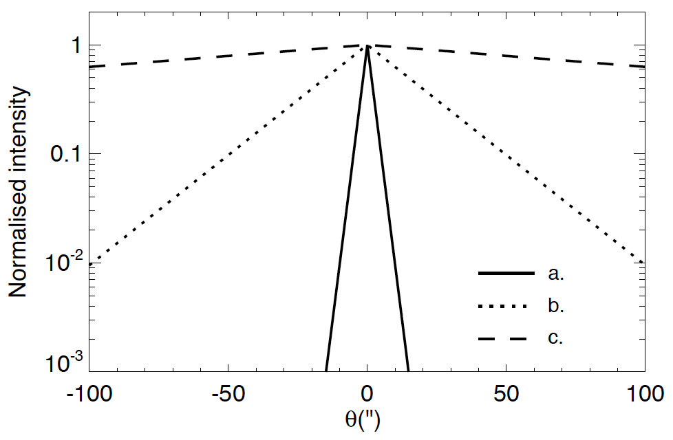
where $z_{\rm d}$ is the scale height of the vertical dust distribution. We introduce the angular distance $\theta\simeq z/D$ and its characteristic value $\theta_{\rm d}\simeq z_{\rm d}/D$. Three scale heights are examined, $z_{\rm d}=$ 0.1, 1 and 10 kpc (scenarios a., b. and c. from Table 1), corresponding to $\theta_{\rm d}\simeq 2,20$ and $200^{\prime\prime}$. Their intrinsic dust profile is shown on Figure 3.

Figure 3: Intrinsic dust profiles (see equation 17) for scenarios a., b. and c. listed in Table 1, corresponding, respectively, to characteristic scale heights of $z_{d}=0.1$, 1 and 10 kpc. These profiles are then convolved with Herschel PSFs to simulate an edge-on galaxy observed in different bands.

We convolve the intrinsic dust profile to the effective PSFs of PACS 70, 100 and 160 $\mu$m and SPIRE 250 and 350 $\mu$m, while keeping the pixel size at $1^{\prime\prime}$. We then make the basic assumption that the dust in the whole galaxy has a temperature of $T_{\rm d}=20$ K and spectral index $\beta=1.6$ (following Planck Collaboration et al. 2014), and rescale the convolved models accordingly.

In order to simulate real data, we add Gaussian statistical noise to the models and consider three different values of signal-to-noise ratio (SNR), $10^{4}$, $10^{2}$, $10$ (scenarios b., b.1 and b.2 from Table 1), with respect to the dust emission at the peak position ($z=0$). These images are then homogenised to the resolution of SPIRE 350 $\mu$m using the four kernel types described in Section 3.1 and resampled with a common pixel size of $10^{\prime\prime}$.

Finally, using a minimum $\chi^{2}$ method, we fit the multi-wavelength data on a pixel-by-pixel basis to a modified blackbody:

$$I_{\nu}=\tau_{\nu_{0}}(\nu/\nu_{0})^{\beta}B_{\nu}(T),$$ (18)

where $\tau_{\nu_{0}}$ is the optical depth at the reference frequency $\nu_{0}$ and $B_{\nu}(T)$ is the blackbody radiation for a grain at temperature $T$.

Figure 4: $\Delta\beta$ parameter as a function of $\Delta T$ for the four kernel types, using an edge-on galaxy with the dust profile b. ($z_{d}=1$ kpc, SNR = $10^{4}$). For a given kernel type, there are 21 data points, each of them corresponding to a measurement on a single pixel along the galaxy profile. The spread thus represents the systematic error on the $\beta-T$ measurement for this kernel type. Error bars on both axis at the centre indicate the statistical errors on $\beta$ and $T$ obtained from the $\chi^{2}$-fitting routine.

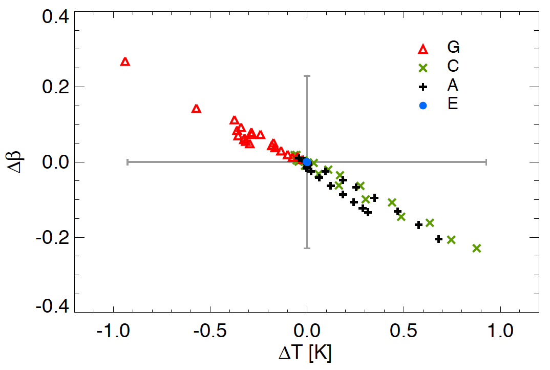
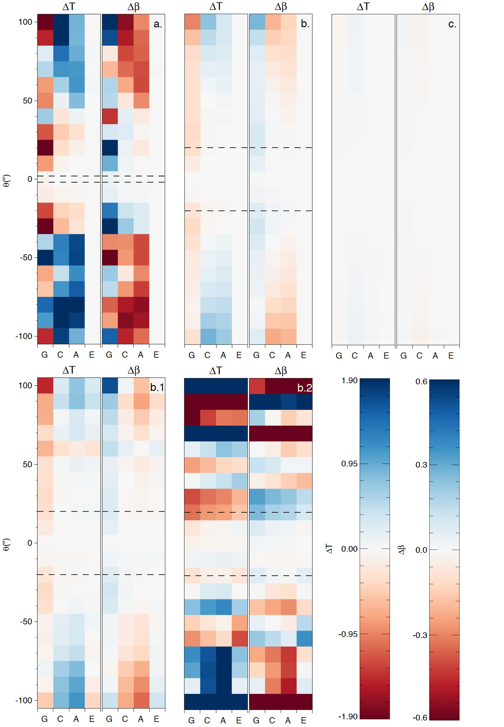
We define $\Delta\beta$ and $\Delta T$ the deviations from the reference dust spectral index $\beta$ and temperature $T_{\rm d}$, respectively. Figure 4 shows $\Delta\beta$ as a function of $\Delta T$ for scenario b. where $z_{\rm d}=1$ kpc and SNR = $10^{4}$, for the different kernel types. Except for the case where effective PSFs are used, systematic discrepancies are present (up to $\Delta T\pm 1$ K and $\Delta\beta\pm 0.3$), comparable in amplitude to the statistical errors (horizontal and vertical bars on Figure 4), and a spurious strong negative correlation appears between dust temperature and $\beta$ parameter.

Table 1: Scale height, $z_{\rm d}$, and signal-to-noise ratio (SNR) adopted for the simulation of dust profiles of an edge-on galaxy.

Scenario	$z_{\rm d}$ (kpc)	SNR
$a.\leavevmode\nobreak\$	0.1	$10^{4}$
$b.\leavevmode\nobreak\$	1.0	$10^{4}$
$c.\leavevmode\nobreak\$	10.0	$10^{4}$
$b.1$	1.0	$10^{2}$
$b.2$	1.0	$10^{1}$

In order to show where this effect is most significant within the galaxy profile, we illustrate on Figure 5 the quantities $\Delta T$ and $\Delta\beta$ at various angular distances from the galaxy centre and for different kernel types (G: Gaussian, C: circular, A: ADGS11, E: effective). Each column thus represents a vertical cut of the modeled galaxy. Dashed lines indicate the characteristic scale height of the intrinsic dust abundance profile. The top three panels show scenarios a., b. and c. where the scale height varies and the SNR is kept constant at $10^{4}$. The two bottom panels show scenarios b.1 and b.2 where the scale height is fixed at 1 kpc and we vary the SNR (see Table 1 for a summary). Each panel of Figure 5 shows the relationship between $\Delta\beta$ and $\Delta T$ just as in Figure 4, and adds the spatial information to the data points.

Depending on the considered dust scale height, deviations from the reference dust temperature and $\beta$ parameter reach $\pm 2$ K and $\pm 0.6$, respectively, with higher deviations for shorter scale heights and at higher galactic latitudes. Regardless of the convolution kernel adopted, the negative correlation is clearly measured for all the pixels in the vertical cut.

Scenarios a., b. and c. show that using the effective kernels, very low ($<1\%$) deviations from the reference values are obtained, while the use of other convolution kernels lead to larger errors for $z\gtrsim z_{\rm d}$. However, as expected, decreasing the level of SNR (scenarios b.1 and b.2), the noise starts to dominate over the signal and very large discrepancies are observed in temperature and $\beta$, regardless of the adopted convolution kernel.

Figure 5: Heat maps of $\Delta T$ and $\Delta\beta$ measured on a simulated edge-on galaxy at various angular distances $\theta$ from the center, as a function of the kernel type used. Each panel represents a scenario from Table 1. Dashed lines indicate the scale height of the dust profile $z_{\rm d}$. This figure highlights the very small scatter in both $\Delta T$ and $\Delta\beta$ when using the kernels with effective PSFs (column E on each plot), until the SNR becomes to low as in panel $b.2$.

4 JWST PSF simulations

To show the reliability of our method for complex-shaped PSFs, we now test our algorithm on simulated PSFs from a telescope with an uncommon optical design. For this purpose, we select the Mid-InfraRed Instrument Imager (MIRI) of the James Webb Space Telescope (JWST, Bouchet et al., 2015). The JWST main mirror being made of several hexagonal mirrors, the optical response of this instrument shows highly non symmetrical features that need to be accounted for in the homogenisation process.

We use WebbPSF (Perrin et al., 2012), the official JWST PSF simulation tool to generate a set of four broadband PSFs of $5^{\prime\prime}\times 5^{\prime\prime}$ centered at $\lambda_{1}=5.6\leavevmode\nobreak\ \mu m$, $\lambda_{2}=11.3\leavevmode\nobreak\ \mu m$, $\lambda_{3}=18.0\leavevmode\nobreak\ \mu m$ and $\lambda_{4}=25.5\leavevmode\nobreak\ \mu m$ in order to cover the spectral range of MIRI. These broadband PSFs were generated from a set of 20 monochromatic ones assuming flat spectral energy distribution of the source, and oversampled at 4 times the pixel size of the detector, corresponding to a pixel scale of 0.11 arcsec. They are displayed on the first column (and top of the second column) of Figure 6.

Using pypher, we then compute three matching kernels, namely, $K_{\lambda_{1},\,\lambda_{4}},K_{\lambda_{2},\,\lambda_{4}}$ and $K_{\lambda_{3},\,\lambda_{4}}$ (following the notation from Section 3.1), to homogenise the first three PSFs to the angular resolution of $E_{\lambda_{4}}$. Using the same procedure as in Section 3.2, we compare these homogenised PSFs to the original one using the residual formalism (15) applied to the MIRI bandpasses. The resulting residual images $R_{\lambda_{1},\,\lambda_{4}},R_{\lambda_{2},\,\lambda_{4}}$ and $R_{\lambda_{3},\,\lambda_{4}}$ are shown on the last column of Figure 6.

Figure 6: Proof of concept of PSF homogenisation for the JWST/MIRI instrument. The PSFs from the first column, respectively at 5.6 $\mu$m, 11.3 $\mu$m and 18.8 $\mu$m, are homogenised to the PSF on top of the second column at 25.5 $\mu$m, using pypher kernels. The resulting homogenised PSFs are shown in the second column. They are visually indistinguishable from the effective one on top. The relative residuals on the right confirm that the central part of the PSF is reconstructed at least to 0.1%.

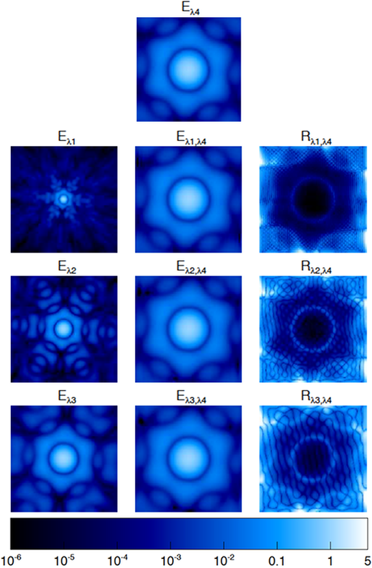
The central region of the residual images, within the two main lobes of the $E_{\lambda_{4}}$ PSF, has a low level of residuals ($\sim 10^{-5}$) in the three configurations Along the image borders, there are some non-negligible residual patches. A quick visual comparison with the homogenised PSFs (central column) shows these patches correspond to extremely faint regions of the PSF ($<10^{-6}$ w.r.t. the peak) and thus having a very low impact in the matching process.

5 Conclusions

In this paper, we propose a new method for the generation of static PSF homogenisation kernels which is applicable for instruments presenting complex PSFs such as recent or future space-born telescopes. The PSF on such optical systems is hardly ever static over the field-of-view, but we restricted the purpose of this paper to the production of homogenization kernels for the study of regions of interest on the image, where the PSF can be considered non-variable. The treatment of the PSF varying over the whole field-of-view of modern instruments cannot be linearized as in this work and requires a very different approach. It will be the subject of a following paper. The application on Herschel/PACS and SPIRE and JWST/MIRI instruments demonstrates the performance of the proposed algorithm in terms of low residuals (better than $10^{-2}-10^{-3}$ and $10^{-5}-10^{-6}$ for observed and simulated PSFs, respectively).

To assess the improvement brought by our algorithm for multi-wavelength studies, we address the estimation of dust temperature and spectral index $\beta$ of astronomical objects using multi-band images taken in the submillimeter spectral range by Herschel. This estimation is made via pixel-by-pixel measurements across these images which have different intrinsic angular resolutions. Homogenisation kernels are thus traditionally used to bring all the images to the same angular resolution. Most of the analysis performed so far use either Gaussian kernels, or the circularised kernels produced by Aniano et al. (2011). However, effective PSFs of space imagers are anisotropic, so these methods are not accurate enough therefore introducing systematic anti-correlation on $\beta$ and temperature measurements with an amplitude which can be larger than the statistical noise. We have checked that using pypher kernels, systematic errors are in any case negligible compared to statistical noise.

Finally, we provide the pypher software (Boucaud, 2016) to compute homogenisation kernels to be used for current and future instruments.

Appendix A The pypher code

A Python code called pypher (Boucaud 2016), that computes the static PSF homogenisation kernels described in this work has been made publicly available and can be retrieved at
https://github.com/aboucaud/pypher.

Once installed, this program can be used through a command-line interface taking as input the PSF images – source and target – as fits files, and specifying the output filename for the kernel,

$ pypher psf_a.fits psf_b.fits kernel_a_to_b.fits

The tunable parameters are

• the regularisation parameter $\mu$ of the Wiener filter (see equation  12) that penalises the high-frequencies, and should be set according to the image that will be homogenised,

• the input PSFs position angle with respect to their image to accurately take into account the shape of both PSF in the homogenisation process.

The program takes less than a second on a single CPU to compute a kernel from two $512\times 512$ PSF images.