Agegraphic dark energy: growth index and cosmological implications

Abstract

We study the main cosmological properties of the agegraphic dark energy model at the expansion and perturbation levels. Initially, using the latest cosmological data we implement a joint likelihood analysis in order to constrain the cosmological parameters. Then we test the performance of the agegraphic dark energy model at the perturbation level and we define its difference from the usual $\Lambda$CDM model. Within this context, we verify that the growth index of matter fluctuations depends on the choice of the considered agegraphic dark energy (homogeneous or clustered). In particular, assuming a homogeneous agegraphic dark energy we find, for the first time, that the asymptotic value of the growth index is $\gamma\approx 5/9$, which is close to that of the usual $\Lambda$ cosmology, $\gamma^{(\Lambda)}\approx 6/11$. Finally, if the distribution of dark energy is clustered then we obtain $\gamma\approx 1/2$ which is $\sim 8\%$ smaller than that of the $\Lambda$CDM model.

1 Introduction

The analysis of various observational data including those of supernovae type Ia (SNIa) (Riess et al., 1998; Perlmutter et al., 1999; Kowalski et al., 2008), cosmic microwave background (CMB) (Komatsu et al., 2009, 2011; Jarosik et al., 2011; Ade et al., 2015), large scale structure and baryonic acoustic oscillation (BAO) (Percival et al., 2010; Tegmark et al., 2004; Cole et al., 2005; Eisenstein et al., 2005; Reid et al., 2012; Blake et al., 2011), high $z$ galaxies (Alcaniz, 2004), high $z$ galaxy clusters (Allen et al., 2004; Wang & Steinhardt, 1998a), weak gravitational lensing (Benjamin et al., 2007; Amendola et al., 2008; Fu et al., 2008) strongly suggest an accelerated expansion of the universe. In the context of General Relativity (GR) the so-called dark energy (hereafter DE), which has a negative pressure, is required in order to interpret the cosmic acceleration. It is interesting to mention that from the overall energy density, only $\sim 30\%$ consists of matter (luminous and dark) while the rest corresponds to DE (see the analysis of Planck2015 (Ade et al., 2015) and references therein).

From the theoretical perspective, over the last two decades, a large family of phenomenological models has been proposed to study the cosmological features of DE. The simplest DE model is the concordance $\rm\Lambda$ cosmology for which the equation of state (EoS) $w_{\rm\Lambda}$ is strictly equal to -1. Despite the fact that the $\Lambda$CDM model fits extremely well the cosmological data it suffers from the fine tuning and the cosmic coincidence problems (Weinberg, 1989; Sahni & Starobinsky, 2000; Carroll, 2001; Padmanabhan, 2003; Copeland et al., 2006). Since the nature of DE has yet unknown, different versions of dynamical DE models have been introduced in order to alleviate the above cosmological issues. Generally speaking, it has been proposed that we cannot entirely understand the nature of dark energy before the establishment of a complete theory of quantum gravity (Witten, 2000). Nevertheless, it is promising that holographic dark energy (HDE) models (Hořava & Minic, 2000; Thomas, 2002) inspired by the principles of quantum gravity can be suggested and may hopefully provide an efficient explanation for the dynamical nature of DE. Specifically, the holographic principle (Susskind, 1995) points out that in a finite-size physical system the number of degrees of freedom should be finite and bounded by the area of its boundary (Cohen et al., 1999). In other words, the total energy of a physical system with size $L$ obeys the following inequality $L^{3}\rho_{\Lambda}\leq Lm_{\rm p}^{2}$, where $\rho_{\rm\Lambda}$ is the quantum zero-point energy density and $m_{\rm p}=1/\sqrt{8\pi G}$ is the Planck mass. Applying the latter arguments to cosmological scales it has been found (see Li, 2004) that the density of the HDE is given by

$$\rho_{\rm d}=3n^{2}m_{\rm p}^{2}L^{-2}\;,$$ (1)

where $n$ is a positive constant and the coefficient $3$ is used for convenience. Obviously, in this case the features of DE strongly depend on the definition of the size $L$ in equation (1). If we assume $L$ to be the Hubble radius $H^{-1}$ then we cannot produce an accelerated expansion of the universe (Hořava & Minic, 2000; Cataldo et al., 2001; Thomas, 2002; Hsu, 2004). Another choice would be to replace $L$ with the particle horizon but again we would not be able to extract cosmic acceleration (Hořava & Minic, 2000; Cataldo et al., 2001; Thomas, 2002; Hsu, 2004). The final choice for $L$ is to use the event horizon (first introduced by Li (2004)). In this case, the HDE model is able to provide cosmic acceleration and it is consistent with observations (Pavón & Zimdahl, 2005; Zimdahl & Pavón, 2007; Sheykhi, 2011). Notice, that the HDE model has been widely investigated in the literature (Huang & Gong, 2004; Huang & Li, 2004; Gong, 2004, 2005; Gong & Zhang, 2005; Zhang & Wu, 2005, 2007; Elizalde et al., 2005; Guberina et al., 2005, 2007; Beltran Almeida & Pereira, 2006; Wang et al., 2005; Shen et al., 2005).

Since the HDE model is obtained by choosing the event horizon length scale, an obvious drawback concerning causality appears in this scenario. Recently, a new DE model, dubbed agegraphic dark energy (ADE) model, has been suggested by Cai (2007) in order to alleviate the above problem. In particular, combining the uncertainty principle in quantum mechanics and the gravitational effects of GR Karolyhazy and his collaborators (Karolyhazy, 1966; F. Karolyhazy & Lukacs, 1982, 1986) made an interesting observation concerning the distance measurement for the Minkowski spacetime through a light-clock Gedanken experiment (see also Maziashvili, 2007a). They found that the distance $t$ in Minkowski spacetime cannot be known to a better accuracy than $\delta t=\beta t_{\rm p}^{2/3}t^{1/3}$, where $\beta$ is a dimensionless constant of order ${\cal O}(1)$ (see also Maziashvili, 2007a). Based on the Karolyhazy relation, Maziashvili (2007a) argued that the energy density of metric fluctuations in the Minkowski spacetime is written as (see also Maziashvili, 2007b)

$$\rho_{d}\sim\frac{1}{t_{p}^{2}t^{2}}\sim\frac{m_{p}}{t^{2}}\;,$$ (2)

where $m_{p}$ and $t_{p}$ are the reduced Plank mass and the Plank time, respectively (see also Sasakura, 1999; Ng & Van Dam, 1994, 1995; Krauss & Turner, 2004; Christiansen et al., 2006; Arzano et al., 2007; Ng, 2007). Using equation (2) Cai (2007) proposed another version of holographic DE the so-called agegraphic dark energy (ADE) in which the time scale $t$ is chosen to be equal with the age of the universe $T=\int^{t}_{0}dt=\int_{0}^{a}\frac{da}{aH}$, with $a$ the scale factor of the universe and $H$ the Hubble parameter. Therefore, the ADE energy density is given by (Cai, 2007)

$$\rho_{d}=\frac{3n^{2}m_{p}^{2}}{T^{2}}$$ (3)

where $n$ is a free parameter and the coefficient $3$ appears for convenience. The present value of the age of universe ($T_{\rm 0}\sim H_{\rm 0}^{-1}$) implies that $n$ is of order ${\cal O}(1)$. It has been shown that the condition $n>1$ is required in order to have cosmic acceleration (Cai, 2007). Although, the ADE scenario does not suffer from the causality problem (Cai, 2007) it faces some problems towards describing the matter-dominated epoch (Wei & Cai, 2008a; Neupane, 2007; Wei & Cai, 2008b). To overcome this issue Wei & Cai (2008a) proposed a new agegraphic dark energy (NADE) model, in which the cosmic time $t$ is replaced by the conformal time $\eta=\int^{t}_{0}{\frac{dt}{a(t)}}=\int^{a}_{0}{\frac{da}{a^{2}H}}$ and thus the energy density in this case becomes (Wei & Cai, 2008a)

$$\rho_{d}=\frac{3n^{2}m_{p}^{2}}{\eta^{2}}\;.$$ (4)

It is interesting to mention that Kim et al. (2008b) showed that the NADE model provides the proper matter-dominated and radiation-dominated epochs, in the case of $n>2.68$ and $n>2.51$, respectively. Also Wei & Cai (2008b) found that the coincidence problem can be alleviated naturally in this model and using the cosmological data (SNIa, CMB etc) they obtained $n=2.716^{+0.111}_{-0.109}$. We would like to point out that the cosmological properties of the ADE and the NADE models can be found in Kim et al. (2008a); Setare & Jamil (2011); Karami et al. (2011); Sheykhi & Setare (2010); Sheykhi (2009, 2010a, 2010b, 2010c); Lee et al. (2008); Jawad et al. (2013); Liu et al. (2012); Zhang et al. (2013); Farajollahi et al. (2012); Zhai et al. (2011); Chen et al. (2011); Sun & Yue (2011); Lemets et al. (2011); Zhang et al. (2010); Liu et al. (2010); Karami & Khaledian (2011); Malekjani & Khodam-Mohammadi (2010); Jamil & Saridakis (2010); Karami et al. (2010); Sheykhi (2010a, b, 2009); Wu et al. (2008); Zhang et al. (2008); Kim et al. (2008b); Neupane (2009); Wei & Cai (2008b).

Furthermore, it is well known that beyond the expansion rate of the universe, DE affects the formation of cosmic structures (Peebles, 1993; Tegmark et al., 2004). Usually, in dynamical DE models with $w_{\rm d}\neq-1$, one can assume that the DE perturbations behave in a similar fashion to matter (Abramo et al., 2007, 2009b, 2009a; Batista & Pace, 2013; Batista, 2014; Mehrabi et al., 2015a; Malekjani et al., 2015; Mehrabi et al., 2015b). In principle, the effective sound speed $c_{\rm eff}^{2}=\delta p_{\rm d}/\delta\rho_{\rm d}$ is introduced in order to describe the DE clustering. In particular, if DE is homogeneous then we have $c^{2}_{\rm eff}=1$, while for clustered DE models we use $c^{2}_{\rm eff}=0$. In the homogeneous case, the sound horizon of DE is close to the Hubble length. This does not hold for $c^{2}_{\rm eff}=0$ (clustered DE) which implies that the perturbations of DE grow, via gravitational instability, in sub-Hubble scales (Armendariz-Picon et al., 1999, 2000; Garriga & Mukhanov, 1999; Akhoury et al., 2011). The growth of matter perturbations in cosmologies where DE is allowed to have clustering has been widely investigated in the literature (Batista & Pace, 2013; Erickson et al., 2002; Bean & Doré, 2004; Hu & Scranton, 2004; Ballesteros & Riotto, 2008; Basilakos et al., 2009a; de Putter et al., 2010; Sapone & Majerotto, 2012; Dossett & Ishak, 2013; Basse et al., 2014; Batista, 2014; Pace et al., 2014; Steigerwald et al., 2014; Mehrabi et al., 2015a, b; Malekjani et al., 2015; Basilakos, 2015; Nesseris & Sapone, 2014).

In this article, following the lines of the above studies, we attempt to investigate the NADE model at the background and perturbation levels. Specifically, we organize the manuscript as follows: in section (2) we start with a brief presentation of the NADE model and in section (3) we investigate the growth of matter perturbations. In section (4), using the latest cosmological data and the growth rate data, we perform a joint likelihood analysis in order to constraint the free parameters of the model. In section (5) we discuss the growth index and finally, we summarize our results in section (6).

2 Background evolution in NADE cosmology

Considering a spatially flat Friedmann-Robertson-Walker (FRW) metric, one can show that the Hubble parameter takes the following form

$$H^{2}=\frac{1}{3m_{p}^{2}}(\rho_{d}+\rho_{m})\;,$$ (5)

where $\rho_{m}$ and $\rho_{d}$ are the energy densities of pressure-less matter and DE respectively. In the case of non-interacting DE models the corresponding densities satisfy the following continuity equations

$$\dot{\rho}_{d}+3H\rho_{d}(1+w_{d})=0$$ (6)

$$\dot{\rho}_{m}+3H\rho_{m}=0,$$ (7)

where $\rho_{m}\propto a^{-3}$ and $\rho_{d}$ is given by equation (4). Therefore, introducing the density parameter $\Omega_{d}\equiv\frac{\rho_{\rm d}}{3m_{p}^{2}H^{2}}$, we obtain

$$\Omega_{d}=\frac{n^{2}}{H^{2}\eta^{2}}.$$ (8)

Of course, one can easily show that equation (5) is reduced to $\Omega_{d}+\Omega_{m}=1$, where $\Omega_{\rm m}\equiv\frac{\rho_{\rm m}}{3m_{p}^{2}H^{2}}$.

Furthermore, differentiating with respect to cosmic time equation (4) and using equations (6) and (8), we derive the corresponding equation of state (EoS) parameter

$$w_{d}=-1+\frac{2}{3na}\sqrt{\Omega_{d}},$$ (9)

where $a(z)=1/(1+z)$ is the scale factor of the universe. Evidently, the above EoS parameter obeys the inequality $w_{d}>-1$ and thus it cannot enter the phantom regime. As expected, at late enough times ($a\rightarrow\infty$) NADE tends to $\Lambda$CDM ($w_{d}\rightarrow-1$). On the other hand, in the matter-dominated epoch, we have $H^{2}\propto\rho_{m}\propto a^{-3}$, which implies $a^{\frac{1}{2}}da\propto dt=ad\eta$. Hence, $\eta\propto a^{\frac{1}{2}}$ and using equations (4), (8) and (6) we easily find $\rho_{d}\propto a^{-1}$, $\Omega_{d}\simeq n^{2}a^{2}/4$ (Wei & Cai, 2008b) and thus $w_{\rm d}\simeq-2/3$. Also, following the notations of Wei & Cai (2008a) one can show (Wei & Cai, 2008a)

$$\frac{d\Omega_{\rm d}}{da}=\frac{\Omega_{d}}{a}(1-\Omega_{d})(3-\frac{2}{na}\sqrt{\Omega_{d}}).$$ (10)

Utilizing the Friedmann equation (5), the continuity equations (6,7) and the dimensionless Hubble parameter $E(a)=H(a)/H_{0}$, we have

$$E^{2}(a)=\frac{\Omega_{m0}a^{-3}+\Omega_{r0}a^{-4}}{1-\Omega_{d}(a)}\;,$$ (11)

where $\Omega_{\rm d}$ satisfies equation (10). We proceed now by solving the system of coupled equations (9,10,11) in order to compute the evolution of the $H(z)$, $w(z)$ and $\Omega_{d}(z)$. As far as the initial conditions are concerned, we start from $a_{\rm i}=0.0005$ which is deep enough in the matter-dominated era (see also Wei & Cai, 2008b). Consequently, the initial value of the DE density parameter is given by $\Omega_{\rm d}(a_{\rm i})=n^{2}a_{\rm i}^{2}/4$.

In Fig.(1) we show the redshift evolution of $\Omega_{d}(z)$ (top panel), $w_{d}(z)$ (middle panel) and $E(z)$ (bottom panel) for different values of the model parameter $n=2.5$ (dashed line), $3.5$ (dotted line) and $4.5$ (dotted dashed line). The concordance $\Lambda$CDM cosmology is also plotted for comparison (see solid line). As expected, the aforementioned cosmological quantities depend on the choice of $n$. Overall, we observe that the EoS parameter remains in the quintessence regime and it lies in the interval $-1\leq w_{d}\leq-\frac{2}{3}$. Also, for large values of $n$, the EoS parameter tends to -1 at the present epoch. The evolution of the DE density parameter shows that for large values of $n>3$, $\Omega_{\rm d}$ is large with respect to that of the concordance $\Lambda$ cosmology. Regarding the normalized Hubble parameter $E(z)$ we see that in the case of $n>3$ we have $E_{\rm NADE}(z)<E_{\Lambda}(z)$, while the opposite holds for $n=2.5$.

Figure 1: The redshift evolution of $\Omega_{d}$ (top panel), $w_{d}$ (middle panel) and $E=H/H_{0}$ (bottom panel). The dashed, dotted and dotted dashed curves correspond to NADE models with $n=2.5$, $n=3.5$ and $n=4.5$, respectively. Notice, that the reference $\Lambda$CDM model is shown by solid curve.

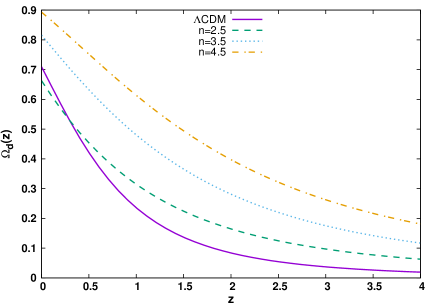
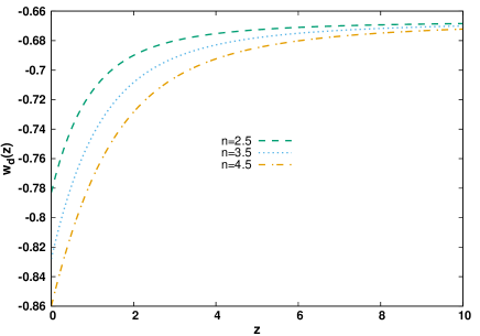
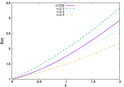
3 growth of perturbations

In this section we proceed with the study of the linear growth of matter perturbations in the NADE model. An important ingredient in this kind of studies is that one can use the so called pseudo-Newtonian approach (Abramo et al., 2007; Pace et al., 2010). It has been shown that in sub-Hubble scales the results of pseudo-Newtonian dynamics are consistent with those of GR (Abramo et al., 2007).

According to Abramo et al. (2009b), the evolution of matter and DE perturbations can be described from the following equations:

$$\dot{\delta}_{m}+\frac{\theta_{m}}{a}=0$$ (12)

$$\dot{\delta}_{d}+(1+w_{d})\frac{\theta_{d}}{a}+3H(c_{\rm eff}^{2}-w_{d})\delta_{d}=0$$ (13)

$$\dot{\theta}_{m}+H\theta_{m}-\frac{k^{2}\phi}{a}=0$$ (14)

$$\dot{\theta}_{d}+H\theta_{d}-\frac{k^{2}c_{\rm eff}^{2}\theta_{d}}{(1+w_{d})a}-\frac{k^{2}\phi}{a}=0$$ (15)

where dot means derivative with respect to cosmic time $t$, $k$ is the wave number of perturbations and $c_{\rm eff}^{2}$ is the effective sound speed. Moreover, the amount of DE clustering strongly depends on the choice of $c_{\rm eff}^{2}$. Indeed, for $c_{\rm eff}^{2}=0$, the perturbations of DE can grow in a similar fashion to matter perturbations (see also Abramo et al., 2009b; Batista & Pace, 2013; Batista, 2014). For this scenario, the fact that the perturbations of DE are affected by the negative pressure implies that the amplitude of DE perturbations is small with respect to that of dark matter fluctuations. On the other hand, for the homogeneous case we have $c_{\rm eff}^{2}=1$ which means that DE perturbations are vanished in sub-Hubble scales.

Also, using the Poisson equation in sub-Hubble scales and with the aid of the above equations we have

$$-\frac{k^{2}}{a^{2}}\phi=\frac{3}{2}H^{2}[\Omega_{m}\delta_{m}+(1+3c_{\rm eff}^{2})\Omega_{d}\delta_{d}].$$ (16)

Replacing equation (16) with equations (15) & (14), eliminating $\theta_{\rm m}$ and $\theta_{\rm d}$ from the system of equations (12,13,14,15) and changing the variables for $t$ to the scale factor $a(t)$ we find

$$\delta_{m}^{{}^{\prime\prime}}+A_{m}\delta_{m}^{{}^{\prime}}+B_{m}\delta_{m}=\frac{3}{2a^{2}}(\Omega_{m}\delta_{m}+\Omega_{d}\delta_{d}),$$ (17)

$$\delta_{d}^{{}^{\prime\prime}}+A_{d}\delta_{d}^{{}^{\prime}}+B_{d}\delta_{d}=\frac{3}{2a^{2}}(1+w_{d})(\Omega_{m}\delta_{m}+\Omega_{d}\delta_{d}),$$ (18)

where we have set $c_{\rm eff}^{2}=0$ and prime denotes derivative with respect to scale factor. Moreover, the corresponding coefficients are written as

$$A_{m}=\frac{3}{2a}(1-w_{d}\Omega_{d});$$

$$B_{m}=0;$$

$$A_{d}=\frac{1}{a}[-3w_{d}-\frac{aw_{d}^{{}^{\prime}}}{1+w_{d}}+\frac{3}{2}(1-w_{d}\Omega_{d})];$$

$$B_{d}=\frac{1}{a^{2}}[-aw_{d}^{{}^{\prime}}+\frac{aw_{d}^{{}^{\prime}}w_{d}}{1+w_{d}}-\frac{1}{2}w_{d}(1-3w_{d}\Omega_{d})].$$

It is important to point out that the growth of DE perturbations strongly depends on the evolution of EoS parameter $w_{\rm d}$. On the other hand, the growth of matter perturbations are directly affected by the perturbations of DE through the system of equations (17) & (18).

Now, we numerically solve the system of Eqs.(17) and (18), using simultaneously the background equations (9), (10) and (11). Concerning the initial conditions we impose the following restriction: at $z_{\rm i}=2000$ ($a_{\rm i}=0.0005$) we use $\delta_{\rm mi}(z_{\rm i})=8\times 10^{-5}$. Additionally, we also adopt the initial conditions provided by Batista & Pace (2013) and Mehrabi et al. (2015c) as follows

$$\delta_{\rm mi}^{\prime}=\frac{\delta_{\rm mi}}{a_{\rm i}}\;,$$ (20)

$$\delta_{\rm di}=\frac{1+w_{\rm di}}{1-3w_{\rm di}}\delta_{\rm mi}\;,$$ (21)

$$\delta_{\rm di}^{\prime}=\frac{4w_{\rm di}^{\prime}}{(1-3w_{\rm di})^{2}}\delta_{\rm mi}+\frac{1+w_{\rm di}}{1-3w_{\rm di}}\delta_{\rm mi}^{\prime}\;,$$ (22)

where $w_{\rm di}=w_{d}(z_{i})$.

As expected, in the case of homogeneous NADE model ( $\delta_{\rm d}\equiv 0$), equation (17) is reduced to the well known differential equation (see also Pace et al., 2010; Mehrabi et al., 2015a)

$$\delta_{m}^{{}^{\prime\prime}}+\frac{3}{2a}(1-w_{\rm d}\Omega_{\rm d})\delta_{m}^{{}^{\prime}}-\frac{3\Omega_{m0}}{2a^{5}E^{2}}\delta_{m}=0,\;.$$ (23)

Therefore, if we allow NADE to have clustering then we solve the system of equations (17) and (18) with the aid of the initial conditions (20, 21 and 22). On the other hand, in the case of homogeneous NADE model we only solve equation (23). Once the matter perturbation $\delta_{\rm m}$ and DE perturbation $\delta_{\rm d}$ are obtained, it is relatively easy to compute the linear growth factor scaled to unity at the present time $D(a)=\delta_{\rm m}(a)/\delta_{\rm m}(a=1)$.

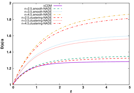
In figure (2), we show the quantity $D(a)/a$ as a function of redshift, $a(z)=1/(1+z)$. As expected, in the Einstein de-Sitter (EdS) model ($\Omega_{\rm m}=1$) the function $D(a)/a$ is always equal to unity. For comparison we also plot $D(a)/a$ for the $\Lambda$CDM cosmology (purple solid curve). Regarding the NADE cosmological model, we plot the evolution of $D(a)/a$ for the following two cases: smooth NADE model ($c_{\rm eff}^{2}=1$) and clustered NADE model ($c_{\rm eff}^{2}=0$), where the model parameter $n$ takes the values $n=2.5,3.5$ and $4.5$. The curve styles and the corresponding colors are mentioned in the caption of figure (2). In general, we find that the amplitude of $D(a)/a$ increases as a function of $n$. We observe that at high $z$ the amplitude of the linear growth of matter fluctuations is larger than the standard $\Lambda$CDM model. Moreover, at high redshifts ($z>2$) $D_{\Lambda}(a)/a$ reaches a plateau which implies that the impact of the cosmological constant on the growth of cosmic structures is practically negligible. However, this is not the case for the NADE cosmological models, namely $D(a)/a$ seems to evolve even at $z\sim 4$. This behavior of the growth factor at high $z$ can be easily interpreted as a small but non-negligible effect of the DE component on the growth of perturbations as we can see in top-panel of figure (1) (see also Batista & Pace, 2013; Malekjani et al., 2015). Note that at the same redshift range and for $n=4.5$ we find that the quantity $D(a)/a$ of the NADE model is $\sim 30\%$ larger than that of the $\Lambda$CDM model. In the case of $n=3.5$ the relative difference is close to $\sim 18\%$ and for $n=2.5$ we have $\sim 4\%$.

Comparing now the smooth and clustered NADE scenarios, we conclude that at high $z$ the growth factor of the latter scenario is small with respect to that of the former model, while prior to the present epoch the growth factor of the smooth NADE model tends to that of the clustered case.

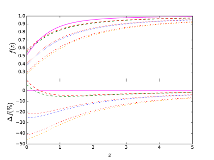
Lastly, we compute the growth rate of clustering in NADE cosmologies. This quantity is defined as the logarithmic derivative of $D$ with respect to $d{\rm ln}a$, $f=d\ln{D(a)}/d\ln{a}$. In figure (3), we show the redshift evolution of $f(z)$ and the fractional difference with respect to that of the concordance $\Lambda$ model,$\Delta f(\%)=(f_{\rm NADE}-f_{\rm\Lambda})/f_{\rm\Lambda}$. As expected, for the reasons developed above we have $f_{\Lambda}(z)\simeq 1$ at high $z$, while in the case of NADE models we find small but not negligible deviations from unity. We also observe that in the redshift range $z\in[0,5]$ we have the following results:

• Smooth NADE model: the relative deviation $\rm\Delta f$ lies in the interval $\sim[5\%,-2\%]$ for $n=2.5$. While for $n=3.5$ and $n=4.5$ we find $\sim[-25\%,-4\%]$ and $\sim[-45\%,-7\%]$ respectively.

• Clustered NADE model: here the relative difference is $\sim[10\%,-2\%]$ for $n=2.5$. While for $n=3.5$ and $n=4.5$ we find $\sim[-20\%,-4\%]$ and $[-40\%,-7\%]$ respectively.

We see that in the framework of clustered NADE the growth rate is somewhat larger than the homogeneous case. We may understand this feature based on the following arguments. In the homogeneous NADE scenario the DE component is uniformly distributed both inside and outside the cosmic structures. In other words DE acts against gravity which implies that more suppression of the growth of matter perturbations is taking place. While, if DE is allowed to clump in a similar manner to dark matter then the total energy of DE can not act against the force of gravity (see also Malekjani et al., 2015).

Figure 2: The redshift evolution of $D(a)/a$. Notice, that the growth factor is normalized to unity at the present time. The purple solid curve shows the concordance $\Lambda$CDM model. In the case of smooth NADE model the corresponding lines are the same to those of figure (1). Red- dashed, red- dotted and red-dotted-dashed curves represent the clustering NADE models with $n=2.5$, $n=3.5$ and $n=4.5$, respectively.

Figure 3: The Redshift evolution of the growth rate of clustering $f(z)$(top panel) and its fractional difference against $\Lambda$CDM model $\rm\Delta f$ (bottom panel). Notice, that the lines are the same to those of figure (2).

4 Observational constraints on the parameter of NADE model

In this section we perform an overall likelihood analysis using the latest cosmological data. Specifically, the total likelihood function is the product of the individual likelihoods:

$${\cal L}_{\rm tot}({\bf p})={\cal L}_{\rm sn}\times{\cal L}_{\rm bao}\times{\cal L}_{\rm cmb}\times{\cal L}_{h}\times{\cal L}_{\rm\rm bbn}\times{\cal L}_{\rm gr}\;,$$ (24)

so the total chi-square $\chi^{2}_{\rm tot}$ is given by:

$$\chi^{2}_{\rm tot}({\bf p})=\chi^{2}_{\rm sn}+\chi^{2}_{\rm bao}+\chi^{2}_{\rm cmb}+\chi^{2}_{h}+\chi^{2}_{\rm bbn}+\chi^{2}_{\rm gr}\;.$$ (25)

For more details regarding the statistical technique, the likelihood functions, the cosmological data (see SNIa, BAO, CMB-shift parameter, $H(z)$, Big Bang Nucleosythesis and growth rate data) with the corresponding covariances, we refer the reader to (Basilakos et al., 2009b; Hinshaw et al., 2013; Mehrabi et al., 2015b; Mehrabi et al., 2015c) The vector ${\bf p}$ contains the free parameters of the particular cosmological model. In the present analysis, the relevant parameters are $(\Omega_{\rm DM},\Omega_{b},\Omega_{r},H_{0},n,\sigma_{8})$. Considering a spatially flat universe, one can obtain $\Omega_{\rm b}=1-\Omega_{d}-\Omega_{\rm DM}-\Omega_{r}$. Notice, that $\Omega_{d}$ is given by Eq. (10) and it only depends on the value of $n$. The radiation density is fixed to $\Omega_{r}=2.469\times 10^{-5}h^{-2}(1.6903)$ (Hinshaw et al., 2013). Therefore, if we use only the expansion data (SNIa, BAOs etc) then the statistical vector becomes ${\bf p}=\{\Omega_{\rm DM},H_{0},n\}$. In the case of background and growth rate data we have ${\bf p}=\{\Omega_{\rm DM},H_{0},n,\sigma_{8}\}$. As far as the evolution of the rms-variance at $R=8h^{-1}$Mpc is concerned we utilize the well known formula $\sigma_{8}(z)=\sigma_{8}\frac{\delta_{m}(z)}{\delta_{m}(z=0)}$. The next step is to use the Markov Chain Monte Carlo (MCMC) procedure in order to find the best fit values and their confidence regions [for a similar analysis see Mehrabi et al. (2015c)].

Figure 4: The overall (geometrical/growth) likelihood contours ($1\sigma$ and $2\sigma$ confidence levels) for various planes. Notice, that in the upper left (upper right) panel we show the results for the smooth NADE (clustered NADE) model. The bottom panel shows the results using only the background (geometrical) data in the likelihood analysis.

Table 1: The best fit values using only the expansion data.

	NADE	$\Lambda$CDM
$\Omega_{\rm DM}$	$0.232\pm 0.011$	$0.2333\pm 0.0098$
$H_{0}$	$65.59\pm 0.64$	$69.68\pm 0.73$
$n$	$2.773\pm 0.056$	$-$
$w_{d}(z=0)$	-0.7966	-1.
$\Omega_{d}(z=0)$	0.7153	0.7208

Table 2: The best fit values using the expansion and the growth rate data.

	Smooth NADE	Clust. NADE	$\Lambda$CDM
$\Omega_{\rm DM}$	$0.232\pm 0.010$	$0.228\pm 0.010$	$0.2321\pm 0.0096$
$H_{0}$	$65.61\pm 0.67$	$65.70\pm 0.68$	$69.73\pm 0.72$
$n$	$2.775\pm 0.053$	$2.795\pm 0.054$	$-$
$\sigma_{8}$	$0.800\pm 0.017$	$0.786\pm 0.017$	$0.773\pm 0.017$
$w_{d}(z=0)$	-0.7967	-0.7971	-1.
$\Omega_{d}(z=0)$	0.7157	0.7192	0.7218

Additionally, we implement the information criteria (IC) in order to test the statistical performance of the models themselves. Specifically, we use the BIC (Schwarz, 1978) and the AIC (Akaike, 1974; Sugiura, 1978) respectively. The BIC formula is given by

$${\rm BIC}=-2\ln{\cal L}_{\rm max}+k\ln N$$ (26)

where ${\cal L}_{\rm max}$ is the maximum likelihood, $k$ is the number of parameters, and $N$ is the number of data points used in the fit. Note that for Gaussian errors, $\chi^{2}_{min}=-2{\cal L}_{\rm max}$, one can prove that the difference in BIC between two models can be simplified to $\Delta BIC=\Delta\chi^{2}_{min}+\Delta k\ln N$. In this context, owing to the fact that $N/k\gg 1$ the AIC is defined as:

$$AIC=-2\ln{\cal L}_{\rm max}+2k$$ (27)

and thus $\Delta AIC=\Delta\chi^{2}_{min}+2\Delta k$. Below we provide our statistical results.

In the case of the expansion data we find:

• for the NADE model, $\chi^{2}_{\rm min}=574.56$, AIC=580.56 and BIC=593.81;

• for the $\Lambda$CDM model, $\chi^{2}_{\rm min}=575.03$, AIC=581.03 and BIC=594.28;

For the background and the growth rate data we have:,

• homogeneous NADE model, $\chi^{2}_{\rm min}=582.28$, AIC=590.28 and BIC=608.07;

• clustered NADE model, $\chi^{2}_{\rm min}=583.05$, AIC=591.03 and BIC= 608.84;

• concordance $\Lambda$CDM model, $\chi^{2}_{\rm min}=582.75$, AIC=590.75 and BIC=608.54.

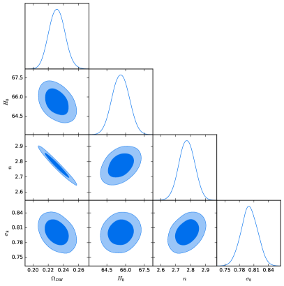
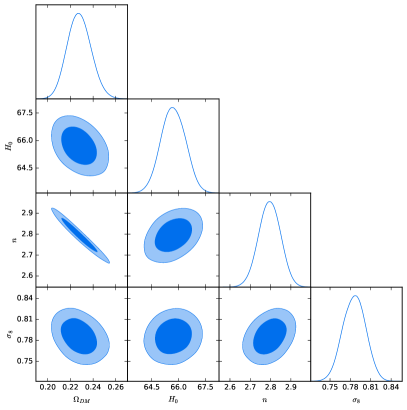
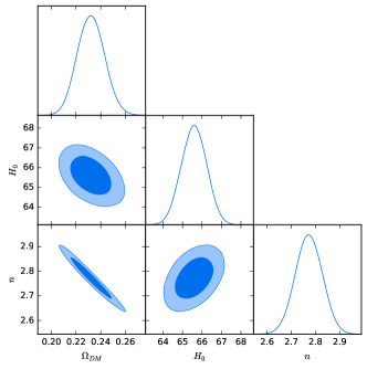
The above results show that NADE (homogeneous or clustered) and $\Lambda$CDM models fit the cosmological data equally well. Moreover, in Tables (1) and (2), one may see a more compact presentation of our constraints including the estimated values of $w_{d}$, $\Omega_{d}(z=0)$ and $n$ (to be used in our growth index analysis). In order to visualize the solution space in Fig.(4) we present the $1\sigma$ and $2\sigma$ confidence contours for various parameter pairs.

In particular, using the background data we find $n=2.773\pm 0.056$. Combining the background data and the growth data we obtain $n=2.775\pm 0.053$ and $n=2.795\pm 0.054$ for smooth and clustered NADE models respectively. $\Omega_{\rm DM}$ is negatively correlated with the model parameter $n$ as expected from the fact that $\Omega_{\rm d}$ in NADE model is correlated with $n^{2}$ by definition. To this end, using the best fit values of Table (1), we can compute the age of universe via the following expression

$$t_{0}=H_{0}^{-1}\int_{0}^{1}\frac{da}{aE(a)}\;.$$ (28)

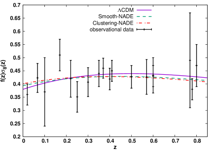
We find $t_{0}^{(\Lambda)}\simeq 13.80$ Gyr and $t_{0}^{(\rm NADE)}\simeq 13.91$ Gyr which are in a good agreement the Planck results ($13.81$ Gyr) (Ade et al., 2015). Concerning the different values of $H_{0}$ between NADE and $\Lambda$CDM the situation is as follows. Technically speaking, in order to obtain the cosmic age of the universe via equation (28), we need to know a priori the Hubble constant and the corresponding value of the integral. Based on the best fit cosmological parameters (see Table 1), we find that the numerical value of the integral is 912.35 and 961.6 for NADE and $\Lambda$CDM respectively. Therefore, a similar value of the cosmic age in NADE and $\Lambda$CDM cosmological models requires that the Hubble constant of the former scenario is small with respect to that of the latter model. Finally, using the best fit cosmological parameters in Fig.(5), we compare the theoretical evolution of the growth rate $f(z)\sigma_{8}(z)$ with observational data. Notice, that criteria of AIC and BIC indicate that both smooth and clustered NADE models together with concordance $\Lambda$CDM model are consistent with the growth data.

Figure 5: Comparison of the observed and theoretical evolution of the growth rate $f(z)\sigma_{8}(z)$. The violet solid, green dashed and red dotted-dashed curves correspond to $\Lambda$CDM, smooth NADE and clustered NADE models. The open squares are the growth data with their error bars.

5 Growth index in NADE model

In this section we concentrate on the growth index of matter fluctuations $\gamma$ which characterizes the growth rate of clustering through the following formula (first introduced by Peebles, 1993)

$$f(z)=\frac{d{\rm ln}\delta_{\rm m}}{d{\rm ln}a}(z)\simeq\Omega^{\gamma}_{m}(z)\;.$$ (29)

In the literature there is a large body of studies which provides the theoretical form of the growth index for various cosmologies, including scalar field DE (Silveira & Waga, 1994; Wang & Steinhardt, 1998b; Linder & Jenkins, 2003; Lue et al., 2004; Linder & Cahn, 2007; Nesseris & Perivolaropoulos, 2008), DGP (Linder & Cahn, 2007; Gong, 2008; Wei, 2008; Fu et al., 2009), Finsler-Randers (Basilakos & Stavrinos, 2013), running vacuum $\Lambda(H)$ (Basilakos & Solà, 2015), $f(R)$ (Gannouji et al., 2009; Tsujikawa et al., 2009), $f(T)$ (Basilakos, 2016) and Holographic dark energy (Mehrabi et al., 2015c).

Now combining equations (16), (12,13,14,15) for $c_{\rm eff}^{2}\neq 0$ and using $\frac{d\delta_{\rm m}}{dt}=aH\frac{d\delta_{\rm m}}{da}$ we find (see also Abramo et al., 2007, 2009b; Mehrabi et al., 2015c)

$$a^{2}\delta_{\rm m}^{\prime\prime}+a\left(3+\frac{\dot{H}}{H^{2}}\right)\delta_{\rm m}^{\prime}=\frac{3}{2}\Omega_{\rm m}\mu\;,$$ (30)

where

$$\frac{{\dot{H}}}{H^{2}}=\frac{d{\rm ln}H}{d{\rm ln}a}=-\frac{3}{2}-\frac{3}{2}{\rm w}_{\rm d}(a)\Omega_{\rm d}(a)\;,$$ (31)

and $\Omega_{\rm d}(a)=1-\Omega_{\rm m}(a)$. Notice, that $\mu(a)$ describes the properties of the NADE model, namely

$$\mu(a)=\left\{\begin{array}[]{cc}1&\mbox{Homogeneous NADE}\\ 1+\frac{\Omega_{\rm d}(a)}{\Omega_{\rm m}(a)}\Delta_{\rm d}(a)(1+3c_{\rm eff}^{2})&\mbox{Clustered NADE}\end{array}\right.$$ (32)

where $\Delta_{\rm d}\equiv\delta_{\rm d}/\delta_{\rm m}$. As expected, if we impose $c_{\rm eff}^{2}=0$ then Eq.(30) boils down to Eq.(17). Also, for the concordance $\Lambda$CDM model we have $\delta_{\rm d}\equiv 0$ by definition.

Moreover, inserting Eq.(29) and Eq.(31) in Eq.(30) we obtain

$$-(1+z)\frac{d\gamma}{dz}{\rm ln}(\Omega_{\rm m})+\Omega_{\rm m}^{\gamma}+3{\rm w}_{\rm d}\Omega_{\rm d}\left(\gamma-\frac{1}{2}\right)+\frac{1}{2}=\frac{3}{2}\Omega_{\rm m}^{1-\gamma}\mu\;.$$ (33)

Concerning the evolution of the growth index one can use the following well known approximation (see also Polarski & Gannouji, 2008; Wu et al., 2009; Belloso et al., 2011; Di Porto et al., 2012; Ishak & Dossett, 2009; Basilakos, 2012; Basilakos & Pouri, 2012)

$$\gamma(a)=\gamma_{0}+\gamma_{1}\left[1-a(z)\right]\;.$$ (34)

Therefore, using Eq.(33) at the present time $z=0$ and taking into account Eq.(34) we find (see also Polarski & Gannouji, 2008)

$$\gamma_{1}=\frac{\Omega_{\rm m0}^{\gamma_{0}}+3{\rm w}_{d0}(\gamma_{0}-\frac{1}{2})\Omega_{\rm d0}+\frac{1}{2}-\frac{3}{2}\Omega_{\rm m0}^{1-\gamma_{0}}\mu_{0}}{{\rm ln}\Omega_{\rm m0}}\;,$$ (35)

where $\mu_{0}=\mu(z=0)$ and ${\rm w}_{d0}={\rm w}_{\rm d}(z=0)$. Obviously, in order to treat the growth index evolution we need to know the value of $\gamma_{0}$. This is given in terms of the asymptotic value of $\gamma(z)$, namely $\gamma_{\infty}\simeq\gamma_{0}+\gamma_{1}$ at high redshifts $z\gg 1$. The analytical formula of $\gamma_{\infty}$ is given by

$$\gamma_{\infty}=\frac{3(M_{0}+M_{1})-2(H_{1}+N_{1})}{2+2X_{1}+3M_{0}}$$ (36)

where the following quantities have been defined:

$$M_{0}=\left.\mu\right|_{\omega=0}\,,\ \ M_{1}=\left.\frac{d\mu}{d\omega}\right|_{\omega=0}$$ (37)

and

$$N_{1}=0\,,\ \ H_{1}=-\frac{X_{1}}{2}=\frac{3}{2}\left.{\rm w_{\rm d}}(a)\right|_{\omega=0}\,.$$ (38)

For more details regarding the above formula we refer the reader to Steigerwald et al. (2014) in which all the cosmological quantities are given in terms of the variable $\omega={\rm ln}\Omega_{\rm m}(a)$. This means that for $z\gg 1$ we have $\Omega_{\rm m}(a)\to 1$ [or $\Omega_{\rm d}(a)\to 0$] and thus $\omega\to 0$. As we have already mentioned in section 2 at large enough redshifts in the matter dominated era we have $\Omega_{d}\simeq n^{2}a^{2}/4$ (Wei & Cai, 2008b) and thus $w_{\infty}\equiv w_{\rm d}(z\gg 1)\simeq-2/3$.

Let us now present our growth index results:

• Homogeneous NADE model: here we have $\mu(a)=1$ ($\Delta_{\rm d}\equiv 0$). Utilizing Eqs.(37) and (38) we obtain

  $$\{M_{0},M_{1},H_{1},X_{1}\}=\{1,0,\frac{3{\rm w}_{\infty}}{2},-3{\rm w}_{\infty}\}$$

  and thus from Eq.(36) we find

  $$\gamma_{\infty}=\frac{3({\rm w}_{\infty}-1)}{6{\rm w}_{\infty}-5}.$$ (39)

  Obviously, for $w_{\infty}\simeq-2/3$ we derive an asymptotic value $\gamma_{\infty}\simeq 5/9$ which is close to that of the $\Lambda$CDM model ($w_{\infty}=-1$), $\gamma_{\infty}^{(\Lambda)}\simeq 6/11$. For comparison we also provide the result of (Mehrabi et al., 2015c) who found $\gamma_{\infty}\simeq 4/7$ in the case of homogeneous HDE model.

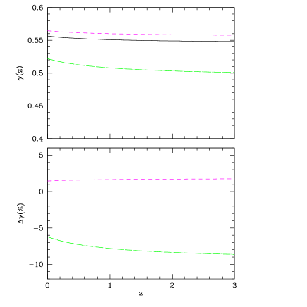
  Substituting now $\gamma_{0}\simeq\gamma_{\infty}-\gamma_{1}$ into Eq.(35) and utilizing the cosmological constraints of Table (2) we obtain $(\gamma_{0},\gamma_{1})\simeq(0.566,-0.01)$. For the $\Lambda$CDM model we have $(\gamma_{0},\gamma_{1})^{(\Lambda)}\simeq(0.557,-0.012)$. In the upper panel of Fig.(6) we show the growth index evolution (34) for the homogeneous NADE (dashed curve) and $\Lambda$CDM models (solid curve) respectively. We see that the evolution of the growth index in homogeneous NADE model is somewhat larger than the usual $\Lambda$CDM cosmological model. Specifically, as we can see from the bottom panel of Fig.(6) the relative difference $[1-\gamma^{(\rm NADE)}/\gamma^{(\Lambda)}]$ is about $\sim 1.7\%$.

• Clustered NADE model: In this case the quantity $\mu(a)$ is given by the second branch of Eq.(32) which implies that we need to treat the form of $\Delta_{\rm d}$. Based on Eq.(21) we arrive at

  $$\Delta_{\rm d}=\frac{1+{\rm w_{d}}}{1-3{\rm w_{d}}}=\frac{1}{3}\frac{\sqrt{\Omega_{\rm d}}}{(2na-\sqrt{\Omega_{\rm d}})}\;.$$ (40)

  Within this context $\mu(a)$ becomes

  $$\mu(a)=1+(1+3c_{\rm eff}^{2})\frac{\Omega_{\rm d}}{1-\Omega_{\rm d}}\frac{1+w_{\rm d}}{1-3w_{\rm d}}\;.$$ (41)

  Therefore, in the matter dominated epoch $\Omega_{d}\simeq n^{2}a^{2}/4$ (or $w_{\rm d}\simeq w_{\infty}\simeq-2/3$) we can easily obtain that $\Delta_{\rm d}\simeq 1/9$ at high $z$ ($a\to 0$ or $\Omega_{\rm d}\to 0$). Thus from Eqs.(37) and (38) we get

  $$\{M_{0},M_{1},H_{1},X_{1}\}=\{1,-\frac{5(1+3c_{\rm eff}^{2})}{27},\frac{3{\rm w}_{\infty}}{2},-3{\rm w}_{\infty}\}$$

  and from Eq.(36) we obtain

  $$\gamma_{\infty}\simeq\frac{40-15c_{\rm eff}^{2}}{81}\;.$$ (42)

  In the case of $c^{2}_{\rm eff}=0$ (fully clustered NADE model) we have $\gamma_{\infty}\simeq 40/81\approx 1/2$ which is lower ($\sim 8\%$) than the theoretically predicted value of the $\Lambda$CDM model $\gamma^{(\Lambda)}_{\infty}\approx 6/11$. Also, we would like to point out that our growth index prediction is larger than that of the clustered HDE model, $\gamma_{\infty}\approx 3/7$ (Mehrabi et al., 2015c).

  Using the above value of $\gamma_{\infty}$, Eq.(35) and the cosmological parameters of Table (2) we obtain $(\gamma_{0},\gamma_{1})\simeq(0.522,-0.028)$. Finally, in the upper panel of Fig(6) we show the evolution of $\gamma(z)$ for the clustered NADE model (dotted dashed curve). In this case, we observe that the growth index deviates with respect to that of the usual $\Lambda$ cosmology. Indeed, the relative deviation lies in the interval $[-6.2\%,-8.6\%]$.

Figure 6: Upper Panel: The growth index versus redshift. The dashed and the dotted dashed lines correspond to homogeneous and clustered NADE models respectively. Notice, that the solid line corresponds to the usual $\Lambda$ cosmology. Bottom Panel: The relative deviation $[1-\gamma(z)/\gamma^{(\Lambda)}(z)]\%$ of the NADE (homogeneous:dashed curve and clustered: dotted dashed curve) models with respect to $\Lambda$CDM.

6 Discussion and Conclusions

Combining the basic uncertainty principle in quantum mechanics together with the gravitational effects of general relativity, Cai (2007) proposed a new model of DE the so-called agegraphic dark energy model (ADE). Replacing the cosmic time $t$ with the conformal time $\eta$, Wei & Cai (2008a, b) introduced in the literature the new agegraphic dark energy (NADE) model in which the corresponding EoS parameter is a function of redshift. The aim of our paper is to investigate the main properties of the NADE model at background and perturbation levels respectively.

The current study was performed by a three-step process. Firstly, solving the system of the main differential equations at the background (Friedmann and continuity) and perturbation levels, we investigated the behavior of the basic cosmological quantities $\{H(z),w(z),\Omega_{\rm d}(z),D(z)\}$ in order to understand the global characteristics of the NADE model (see Fig.1). We verified that the EoS parameter remains in the quintessence regime and it lies in the interval $-1\leq w_{d}\leq-\frac{2}{3}$. Notice, that for large values of $n$ the current value of the EoS parameter tends to -1. As expected, the cosmic expansion depends on the choice of $n$. In particular, we found that for large values of $n>3$, the parameter $\Omega_{\rm d}(z)$ of the NADE model strongly deviates from that of $\Lambda$CDM. In this context we have that the Hubble parameters obey: $H_{\rm NADE}(z)<H_{\Lambda}(z)$. Also, we found that the growth factor $D_{\rm NADE}(z)$ seems to evolve at high redshifts $z>2$ and the amplitude of $D_{\rm NADE}(z)$ increases as a function of $n$. Note that at the same redshift range $D_{\Lambda}(z)$ reached a plateau. Potentially, the latter behavior of $D(z)$ can be used to distinguish between NADE and $\Lambda$CDM at perturbation level.

Secondly, we performed a joint statistical analysis, involving the latest geometrical data (SNe type Ia, CMB shift parameter and BAO etc) and growth data and found that the combined statistical analysis, within the context of flat FRW space, can place tight constrains on the main cosmological parameters giving the reader the opportunity to appreciate the precision of our statistical results. In particular, we found $n=2.775\pm 0.053$ ($\sigma_{8}=0.800\pm 0.017$) and $n=2.795\pm 0.054$ ($\sigma_{8}=0.786\pm 0.017$) for homogeneous and inhomogeneous (DE is allowed to clump) NADE models respectively. Notice, that the present value of $\Omega_{m}$ is close to 0.29 in all cases. It is interesting to mention that the above constraints are in agreement with those of Wei & Cai (2008b) (see also Wei, 2009; Zhang et al., 2013). Using the aforementioned cosmological parameters we found that the age of the universe is $t_{0}^{(\rm NADE)}\simeq 13.91$ Gyr which differs from that of the Planck (Ade et al., 2015) by $\sim 1\%$. Lastly, using the basic information criteria (AIC and BIC), we concluded that both smooth and clustered NADE scenarios as well as the $\Lambda$CDM model fit the observationally data equally well.

Thirdly, we studied the performance of NADE model at the perturbation level. Specifically, following the methodology of (Steigerwald et al., 2014) we estimated for the NADE model the asymptotic value of the growth index of linear matter fluctuations ($\gamma$). Considering a homogeneous NADE model we found $\gamma\approx 5/9$ which is close to that of the traditional $\Lambda$ cosmology $\gamma^{(\Lambda)}\approx 6/11$. On the other hand, if we allow clustering in NADE then we obtained $\gamma\approx 1/2$, which is $\sim 8\%$ smaller than that of the $\Lambda$CDM model. Finally, we extended the growth analysis in the case where $\gamma$ varies with redshift and found that the $\gamma(z)$ is quite large with respect to that of the clustered NADE scenario. This implies that the clustered DE scenario can be differentiated from the other two models on the basis of the growth index evolution.

References

- Abramo et al. (2007) Abramo L. R., Batista R. C., Liberato L., Rosenfeld R., 2007, Journal of Cosmology and Astro-Particle Physics, 11, 12
- Abramo et al. (2009a) Abramo L. R., Batista R. C., Liberato L., Rosenfeld R., 2009a, Phys. Rev. D, 79, 023516
- Abramo et al. (2009b) Abramo L. R., Batista R. C., Liberato L., Rosenfeld R., 2009b, Phys. Rev., D79, 023516
- Ade et al. (2015) Ade P. A. R., et al., 2015
- Akaike (1974) Akaike H., 1974, IEEE Transactions of Automatic Control, 19, 716
- Akhoury et al. (2011) Akhoury R., Garfinkle D., Saotome R., 2011, JHEP, 04, 096
- Alcaniz (2004) Alcaniz J. S., 2004, Phys. Rev., D69, 083521
- Allen et al. (2004) Allen S. W., Schmidt R. W., Ebeling H., Fabian A. C., van Speybroeck L., 2004, Mon. Not. Roy. Astron. Soc., 353, 457
- Amendola et al. (2008) Amendola L., Kunz M., Sapone D., 2008, JCAP, 0804, 013
- Armendariz-Picon et al. (1999) Armendariz-Picon C., Damour T., Mukhanov V. F., 1999, Phys. Lett., B458, 209
- Armendariz-Picon et al. (2000) Armendariz-Picon C., Mukhanov V. F., Steinhardt P. J., 2000, Phys. Rev. Lett., 85, 4438
- Arzano et al. (2007) Arzano M., Kephart T. W., Ng Y. J., 2007, Phys. Lett., B649, 243
- Ballesteros & Riotto (2008) Ballesteros G., Riotto A., 2008, Phys. Lett. B, 668, 171
- Basilakos (2012) Basilakos S., 2012, Int. J. Mod. Phys., D21, 1250064
- Basilakos (2015) Basilakos S., 2015, Mon. Not. Roy. Astron. Soc., 449, 2151
- Basilakos (2016) Basilakos S., 2016, Phys. Rev., D93, 083007
- Basilakos & Pouri (2012) Basilakos S., Pouri A., 2012, Mon. Not. Roy. Astron. Soc., 423, 3761
- Basilakos & Solà (2015) Basilakos S., Solà J., 2015, Phys. Rev., D92, 123501
- Basilakos & Stavrinos (2013) Basilakos S., Stavrinos P., 2013, Phys. Rev., D87, 043506
- Basilakos et al. (2009a) Basilakos S., Bueno Sanchez J., Perivolaropoulos L., 2009a, Phys. Rev. D, 80, 043530
- Basilakos et al. (2009b) Basilakos S., Plionis M., Sola J., 2009b, Phys. Rev., D80, 083511
- Basse et al. (2014) Basse T., Bjaelde O. E., Hamann J., Hannestad S., Wong Y. Y., 2014, JCAP, 1405, 021
- Batista (2014) Batista R. C., 2014, Phys. Rev. D, 89, 123508
- Batista & Pace (2013) Batista R., Pace F., 2013, JCAP, 1306, 044
- Bean & Doré (2004) Bean R., Doré O., 2004, Phys. Rev. D, 69, 083503
- Belloso et al. (2011) Belloso A. B., Garcia-Bellido J., Sapone D., 2011, JCAP, 1110, 010
- Beltran Almeida & Pereira (2006) Beltran Almeida J. P., Pereira J. G., 2006, Phys. Lett., B636, 75
- Benjamin et al. (2007) Benjamin J., et al., 2007, Mon. Not. Roy. Astron. Soc., 381, 702
- Blake et al. (2011) Blake C., Brough S., Colless M., Contreras C., Couch W., et al., 2011, MNRAS, 415, 2876
- Cai (2007) Cai R. G., 2007, Phys. Lett. B, 657, 228
- Carroll (2001) Carroll S. M., 2001, Living Reviews in Relativity, 380, 1
- Cataldo et al. (2001) Cataldo M., Cruz N., del Campo S., Lepe S., 2001, Physics Letters B, 509, 138
- Chen et al. (2011) Chen Y., Zhu Z.-H., Xu L., Alcaniz J. S., 2011, Phys. Lett., B698, 175
- Christiansen et al. (2006) Christiansen W. A., Ng Y. J., van Dam H., 2006, Phys. Rev. Lett., 96, 051301
- Cohen et al. (1999) Cohen A. G., Kaplan D. B., Nelson A. E., 1999, Physical Review Letters, 82, 4971
- Cole et al. (2005) Cole S., et al., 2005, MNRAS, 362, 505
- Copeland et al. (2006) Copeland E. J., Sami M., Tsujikawa S., 2006, IJMP, D15, 1753
- Di Porto et al. (2012) Di Porto C., Amendola L., Branchini E., 2012, Mon. Not. Roy. Astron. Soc., 419, 985
- Dossett & Ishak (2013) Dossett J., Ishak M., 2013, Phys. Rev. D, D88, 103008
- Eisenstein et al. (2005) Eisenstein D. J., et al., 2005, ApJ, 633, 560
- Elizalde et al. (2005) Elizalde E., Nojiri S., Odintsov S. D., Wang P., 2005, Phys. Rev., D71, 103504
- Erickson et al. (2002) Erickson J. K., Caldwell R., Steinhardt P. J., Armendariz-Picon C., Mukhanov V. F., 2002, Phys. Rev. Lett., 88, 121301
- F. Karolyhazy & Lukacs (1982) F. Karolyhazy A. F., Lukacs B., 1982, Physics as natural Philosophy. MIT Press
- F. Karolyhazy & Lukacs (1986) F. Karolyhazy A. F., Lukacs B., 1986, Quantum Concepts in Space and Time. Clarendon Press, Oxford
- Farajollahi et al. (2012) Farajollahi H., Ravanpak A., Fadakar G. F., 2012, Phys. Lett., B711, 225
- Fu et al. (2008) Fu L., et al., 2008, Astron. Astrophys., 479, 9
- Fu et al. (2009) Fu X.-y., Wu P.-x., Yu H.-w., 2009, Phys. Lett., B677, 12
- Gannouji et al. (2009) Gannouji R., Moraes B., Polarski D., 2009, JCAP, 0902, 034
- Garriga & Mukhanov (1999) Garriga J., Mukhanov V. F., 1999, Phys. Lett., B458, 219
- Gong (2004) Gong Y., 2004, Phys. Rev. D, 70, 064029
- Gong (2005) Gong Y., 2005, Classical and Quantum Gravity, 22, 2121
- Gong (2008) Gong Y., 2008, Phys. Rev., D78, 123010
- Gong & Zhang (2005) Gong Y., Zhang Y. Z., 2005, Phys. Rev. D, 72, 043518
- Guberina et al. (2005) Guberina B., Horvat R., Stefancic H., 2005, JCAP, 0505, 001
- Guberina et al. (2007) Guberina B., Horvat R., Nikolic H., 2007, JCAP, 0701, 012
- Hinshaw et al. (2013) Hinshaw G., et al., 2013, ApJS, 208, 19
- Hořava & Minic (2000) Hořava P., Minic D., 2000, Physical Review Letters, 85, 1610
- Hsu (2004) Hsu S. D. H., 2004, Physical Letters B, 594, 13
- Hu & Scranton (2004) Hu W., Scranton R., 2004, Phys. Rev. D, 70, 123002
- Huang & Gong (2004) Huang Q.-G., Gong Y.-G., 2004, JCAP, 0408, 006
- Huang & Li (2004) Huang Q. G., Li M., 2004, J. Cosmology Astropart. Phys., 8, 013
- Ishak & Dossett (2009) Ishak M., Dossett J., 2009, Phys. Rev., D80, 043004
- Jamil & Saridakis (2010) Jamil M., Saridakis E. N., 2010, JCAP, 1007, 028
- Jarosik et al. (2011) Jarosik N., et al., 2011, ApJS, 192, 14
- Jawad et al. (2013) Jawad A., Chattopadhyay S., Pasqua A., 2013, Eur. Phys. J. Plus, 128, 88
- Karami & Khaledian (2011) Karami K., Khaledian M. S., 2011, JHEP, 03, 086
- Karami et al. (2010) Karami K., Khaledian M. S., Felegary F., Azarmi Z., 2010, Phys. Lett., B686, 216
- Karami et al. (2011) Karami K., Sheykhi A., Jamil M., Felegary F., Soltanzadeh M. M., 2011, Europhys. Lett., 93, 69001
- Karolyhazy (1966) Karolyhazy F., 1966, Nuovo Cim., A42, 390
- Kim et al. (2008a) Kim Y.-W., Lee H. W., Myung Y. S., Park M.-I., 2008a, Mod. Phys. Lett., A23, 3049
- Kim et al. (2008b) Kim K. Y., Lee H. W., Myung Y. S., 2008b, Phys. Lett., B660, 118
- Komatsu et al. (2009) Komatsu E., Dunkley J., Nolta M. R., et al. 2009, ApJS, 180, 330
- Komatsu et al. (2011) Komatsu E., Smith K. M., Dunkley J., et al. 2011, ApJS, 192, 18
- Kowalski et al. (2008) Kowalski M., Rubin D., Aldering G., et al. 2008, ApJ, 686, 749
- Krauss & Turner (2004) Krauss L. M., Turner M. S., 2004, Sci. Am., 291, 52
- Lee et al. (2008) Lee H. W., Kim K. Y., Myung Y. S., 2008, Mod. Phys. Lett., A23, 1366
- Lemets et al. (2011) Lemets O. A., Yerokhin D. A., Zazunov L. G., 2011, JCAP, 1101, 007
- Li (2004) Li M., 2004, Physics Letters B, 603, 1
- Linder & Cahn (2007) Linder E. V., Cahn R. N., 2007, Astropart. Phys., 28, 481
- Linder & Jenkins (2003) Linder E. V., Jenkins A., 2003, Mon. Not. Roy. Astron. Soc., 346, 573
- Liu et al. (2010) Liu X.-L., Zhang J., Zhang X., 2010, Phys. Lett., B689, 139
- Liu et al. (2012) Liu X.-M., Zhai Z.-X., Xiao K., Liu W.-B., 2012, Eur. Phys. J., C72, 2057
- Lue et al. (2004) Lue A., Scoccimarro R., Starkman G. D., 2004, Phys. Rev., D69, 124015
- Malekjani & Khodam-Mohammadi (2010) Malekjani M., Khodam-Mohammadi A., 2010, Int. J. Mod. Phys., D19, 1857
- Malekjani et al. (2015) Malekjani M., Naderi T., Pace F., 2015, Mon. Not. Roy. Astron. Soc., 453, 4148
- Maziashvili (2007a) Maziashvili M., 2007a, Int. J. Mod. Phys., D16, 1531
- Maziashvili (2007b) Maziashvili M., 2007b, Phys. Lett., B652, 165
- Mehrabi et al. (2015a) Mehrabi A., Malekjani M., Pace F., 2015a, Astrophys. Space Sci., 356, 129
- Mehrabi et al. (2015b) Mehrabi A., Basilakos S., Pace F., 2015b, MNRAS, 452, 2930
- Mehrabi et al. (2015c) Mehrabi A., Basilakos S., Malekjani M., Davari Z., 2015c, Phys. Rev., D92, 123513
- Nesseris & Perivolaropoulos (2008) Nesseris S., Perivolaropoulos L., 2008, Phys. Rev., D77, 023504
- Nesseris & Sapone (2014) Nesseris S., Sapone D., 2014, ArXiv e-prints, 1409.3697
- Neupane (2007) Neupane I. P., 2007, Phys. Rev., D76, 123006
- Neupane (2009) Neupane I. P., 2009, Phys. Lett., B673, 111
- Ng (2007) Ng Y. J., 2007, Phys. Lett., B657, 10
- Ng & Van Dam (1994) Ng Y. J., Van Dam H., 1994, Mod. Phys. Lett., A9, 335
- Ng & Van Dam (1995) Ng Y. J., Van Dam H., 1995, Mod. Phys. Lett., A10, 2801
- Pace et al. (2010) Pace F., Waizmann J. C., Bartelmann M., 2010, MNRAS, 406, 1865
- Pace et al. (2014) Pace F., Batista R. C., Del Popolo A., 2014, MNRAS, 445, 648
- Padmanabhan (2003) Padmanabhan T., 2003, Phys. Rep., 380, 235
- Pavón & Zimdahl (2005) Pavón D., Zimdahl W., 2005, Physical Letters B, 628, 206
- Peebles (1993) Peebles P. J. E., 1993, Principles of physical cosmology. Princeton University Press
- Percival et al. (2010) Percival W. J., Reid B. A., Eisenstein D. J., et al. 2010, MNRAS, 401, 2148
- Perlmutter et al. (1999) Perlmutter S., Aldering G., Goldhaber G., et al. 1999, ApJ, 517, 565
- Polarski & Gannouji (2008) Polarski D., Gannouji R., 2008, Phys. Lett., B660, 439
- Reid et al. (2012) Reid B. A., Samushia L., White M., Percival W. J., Manera M., et al., 2012, MNRAS, 426, 2719
- Riess et al. (1998) Riess A. G., Filippenko A. V., Challis P., et al. 1998, AJ, 116, 1009
- Sahni & Starobinsky (2000) Sahni V., Starobinsky A. A., 2000, IJMPD, 9, 373
- Sapone & Majerotto (2012) Sapone D., Majerotto E., 2012, Phys. Rev. D, 85, 123529
- Sasakura (1999) Sasakura N., 1999, Prog. Theor. Phys., 102, 169
- Schwarz (1978) Schwarz G., 1978, Annals of Statistics, 6, 461
- Setare & Jamil (2011) Setare M. R., Jamil M., 2011, Gen. Rel. Grav., 43, 293
- Shen et al. (2005) Shen J.-y., Wang B., Abdalla E., Su R.-K., 2005, Phys. Lett., B609, 200
- Sheykhi (2009) Sheykhi A., 2009, Phys. Lett., B680, 113
- Sheykhi (2010a) Sheykhi A., 2010a, Phys. Rev., D81, 023525
- Sheykhi (2010b) Sheykhi A., 2010b, JCAP, 1009, 017
- Sheykhi (2010c) Sheykhi A., 2010c, Phys. Lett., B682, 329
- Sheykhi (2011) Sheykhi A., 2011, Phys. Rev., D84, 107302
- Sheykhi & Setare (2010) Sheykhi A., Setare M. R., 2010, Int. J. Theor. Phys., 49, 2777
- Silveira & Waga (1994) Silveira V., Waga I., 1994, Phys. Rev., D50, 4890
- Steigerwald et al. (2014) Steigerwald H., Bel J., Marinoni C., 2014, JCAP, 1405, 042
- Sugiura (1978) Sugiura N., 1978, Communications in Statistics A, Theory and Methods, 7, 13
- Sun & Yue (2011) Sun C.-Y., Yue R.-H., 2011, Phys. Rev., D83, 107302
- Susskind (1995) Susskind L., 1995, Journal of Mathematical Physics, 36, 6377
- Tegmark et al. (2004) Tegmark M., et al., 2004, Phys. Rev. D, 69, 103501
- Thomas (2002) Thomas S., 2002, Physical Review Letters, 89, 081301
- Tsujikawa et al. (2009) Tsujikawa S., Gannouji R., Moraes B., Polarski D., 2009, Phys. Rev., D80, 084044
- Wang & Steinhardt (1998a) Wang L., Steinhardt P. J., 1998a, ApJ, 508, 483
- Wang & Steinhardt (1998b) Wang L.-M., Steinhardt P. J., 1998b, Astrophys. J., 508, 483
- Wang et al. (2005) Wang B., Abdalla E., Su R.-K., 2005, Phys. Lett., B611, 21
- Wei (2008) Wei H., 2008, Phys. Lett., B664, 1
- Wei (2009) Wei H., 2009, Eur. Phys. J., C60, 449
- Wei & Cai (2008a) Wei H., Cai R.-G., 2008a, Phys. Lett., B660, 113
- Wei & Cai (2008b) Wei H., Cai R.-G., 2008b, Phys. Lett., B663, 1
- Weinberg (1989) Weinberg S., 1989, Reviews of Modern Physics, 61, 1
- Witten (2000) Witten E., 2000, in Sources and detection of dark matter and dark energy in the universe. Proceedings, 4th International Symposium, DM 2000, Marina del Rey, USA, February 23-25, 2000. pp 27–36 (arXiv:hep-ph/0002297), http://www.slac.stanford.edu/spires/find/books/www?cl=QB461:I57:2000
- Wu et al. (2008) Wu J.-P., Ma D.-Z., Ling Y., 2008, Phys. Lett., B663, 152
- Wu et al. (2009) Wu P., Yu H. W., Fu X., 2009, JCAP, 0906, 019
- Zhai et al. (2011) Zhai Z.-X., Zhang T.-J., Liu W.-B., 2011, JCAP, 1108, 019
- Zhang & Wu (2005) Zhang X., Wu F.-Q., 2005, Phys. Rev., D72, 043524
- Zhang & Wu (2007) Zhang X., Wu F.-Q., 2007, Phys. Rev., D76, 023502
- Zhang et al. (2008) Zhang X., Zhang J., Liu H., 2008, Eur. Phys. J., C54, 303
- Zhang et al. (2010) Zhang J., Zhang L., Zhang X., 2010, Phys. Lett., B691, 11
- Zhang et al. (2013) Zhang J.-F., Li Y.-H., Zhang X., 2013, Eur. Phys. J., C73, 2280
- Zimdahl & Pavón (2007) Zimdahl W., Pavón D., 2007, Classical and Quantum Gravity, 24, 5461
- de Putter et al. (2010) de Putter R., Huterer D., Linder E. V., 2010, Phys. Rev. D, 81, 103513