Long-Term X-RAY Variability of Typical Active Galactic Nuclei in the Distant Universe

Abstract

We perform long-term ($\approx 15$ yr, observed-frame) X-ray variability analyses of the 68 brightest radio-quiet active galactic nuclei (AGNs) in the 6 Ms Chandra Deep Field-South (CDF-S) survey; the majority are in the redshift range of 0.6–3.1, providing access to penetrating rest-frame X-rays up to $\approx 10-30$ keV. Twenty-four of the 68 sources are optical spectral type I AGNs, and the rest (44) are type II AGNs. The time scales probed in this work are among the longest for X-ray variability studies of distant AGNs. Photometric analyses reveal widespread photon-flux variability: $90\%$ of AGNs are variable above a 95% confidence level, including many X-ray obscured AGNs and several optically classified type II quasars. We characterize the intrinsic X-ray luminosity ($L_{\rm{X}}$) and absorption ($N_{\rm{H}}$) variability via spectral fitting. Most (74%) sources show $L_{\rm{X}}$ variability; the variability amplitudes are generally smaller for quasars. A Compton-thick candidate AGN shows variability of its high-energy X-ray flux, indicating the size of reflecting material to be $\mathrel{\hbox to0.0pt{\lower 4.0pt\hbox{\hskip 1.0pt$\sim$}\hss}\raise 1.0pt\hbox{$<$}}0.3$ pc. $L_{\rm{X}}$ variability is also detected in a broad absorption line (BAL) quasar. The $N_{\rm{H}}$ variability amplitude for our sample appears to rise as time separation increases. About 16% of sources show $N_{\rm{H}}$ variability. One source transitions from an X-ray unobscured to obscured state while its optical classification remains type I; this behavior indicates the X-ray eclipsing material is not large enough to obscure the whole broad-line region.

1. Introduction

Variability studies are valuable in probing the physical properties of active galactic nuclei (AGNs) (e.g., Ulrich et al., 1997; Peterson, 2001). Simple light-travel time arguments enable a first-order estimation of the sizes of the radiation-emitting regions. More detailed reverberation-based studies provide size estimates of different components; e.g., the correlations among multi-color light curves give temperature profiles of accretion disks (e.g., Fausnaugh et al., 2015); time lags between the continuum and emission lines indicate the radius of broad-line region (BLR) (e.g., Peterson, 2014); and delays of the near-infrared (NIR) dust emission compared to the optical disk emission constrain the inner size of the dusty torus (e.g., Koshida et al., 2014). Changes in absorption provide insights into the absorbing matter: e.g., variability of broad absorption line (BAL) troughs reveals wind properties (e.g., Filiz Ak et al., 2013), and variations of optical reddening and X-ray absorption indicate a clumpy nature of the ambient gas (e.g., Goodrich, 1995; Netzer, 2015). In AGN jet studies, the rapid variability of blazars’ $\gamma$-ray emission often indicates small emitting regions and the relativistically beamed nature of the radiation (e.g., Begelman et al., 2008; Abdo et al., 2010).

X-ray variability is of great importance among AGN variability studies. In AGN spectral energy distributions (SEDs), luminous X-ray emission is almost universal and often a significant contributor to the total source power (e.g., Gibson et al., 2008). X-ray variability is generally of larger amplitude and more rapid compared to that at longer wavelengths (e.g., Ulrich et al., 1997; Peterson, 2001), indicating that the high-energy radiation is probing the immediate vicinity of the supermassive black hole (SMBH). For the majority population of obscured AGNs, the penetrating nature of X-rays often allows variability studies of emission as well as absorption (e.g., Puccetti et al., 2014; Hernández-García et al., 2015).

Intensive X-ray variability analyses have been performed for the radio-quiet AGNs that are the majority population. Studies of broadband X-ray continuum variability have found that local Seyfert 1s (i.e., unabsorbed AGNs) are highly X-ray variable, and that the variation amplitude generally decreases as luminosity increases (e.g., Nandra et al., 1997; Ponti et al., 2012). This amplitude-luminosity relation might be a byproduct of a primary amplitude-SMBH mass relation (e.g., Ponti et al., 2012, and references therein). Seyfert 2s, especially the Compton-thick (obscuration column density $N_{\rm{H}}$ $\mathrel{\hbox to0.0pt{\lower 4.0pt\hbox{\hskip 1.0pt$\sim$}\hss}\raise 1.0pt\hbox{$>$}}1.5\times 10^{24}$ cm^-2) ones, tend to be less X-ray variable than Seyfert 1s at least on time scales of hours or less (e.g., Turner et al., 1997; Awaki et al., 2006; Hernández-García et al., 2015). Studies of distant AGNs, such as optically selected quasars, have also reported prevalent X-ray variability (e.g., Gibson & Brandt 2012, G12 hereafter; Shemmer et al. 2014) and a similar amplitude-luminosity relation as seen in local Seyfert galaxies (e.g., Almaini et al., 2000; Paolillo et al., 2004; Papadakis et al., 2008; Lanzuisi et al., 2014). Compared to the X-ray continuum, the narrow Fe K emission-line components are less variable (e.g., Markowitz et al., 2003), consistent with the picture that they originate from the outer disk or torus. Recent works (e.g., Zoghbi et al., 2012; Kara et al., 2013) reveal short-timescale (minutes) lags of the broad Fe K emission-line components relative to the continuum, suggesting they are emitted from the inner disk illuminated by the continuum X-rays. X-ray photoelectric absorption variability has also been found in many Seyfert 2s (e.g., Risaliti et al., 2002, 2007). Modeling of the observed absorption variations suggests this absorption originates in gas clouds in the BLR or torus orbiting the central source (e.g., Maiolino et al., 2010; Markowitz et al., 2014; Torricelli-Ciamponi et al., 2014; Netzer, 2015). X-ray absorption variability has also been widely investigated in warm absorbers, BAL quasar winds, and ultra fast outflows (UFOs), usefully characterizing wind properties (e.g., Chartas et al., 2009; Matt et al., 2011; Saez et al., 2012; King & Pounds, 2015; Scott et al., 2015).

The X-ray variability of AGNs generally shows a red-noise power spectral density (PSD, e.g., Uttley et al., 2002); i.e., AGNs vary by larger amplitudes on longer time scales. X-ray variability analyses on longer time scales thus have a better chance of detecting variability in data of a given signal-to-noise ratio, thereby providing physical insights about the nature of the AGNs. Long-term variability studies are also helpful in evaluating the effects of AGN variability upon statistical inferences made about source populations in single-epoch X-ray surveys. Furthermore, long-term X-ray variability studies might capture novel AGN phenomena; e.g., “changing-look” events (e.g., Matt et al., 2003; Ricci et al., 2016), emission-state changes (e.g., Miniutti et al., 2012), and torus-eclipse events (e.g., Markowitz et al., 2014). Variability analyses on time scales of years can probe the regime of mechanical instabilities of the accretion disk (assuming a $\sim 10^{8}\ \rm M_{\sun}$ SMBH; see, e.g., Peterson 2001).

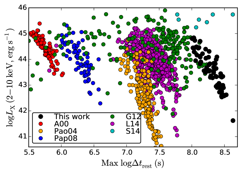
Motivated by the importance of X-ray variability studies, especially on long time scales, we here explore the X-ray variability of the X-ray brightest radio-quiet AGNs in the Chandra Deep Field-South (CDF-S; e.g., Xue et al. 2011; B. Luo et al., in preparation, L16 hereafter). We take advantage of the data products from the observations by Chandra of the CDF-S. The observations span $\approx 15$ yr and are well separated, enabling us to characterize long-term variability properties of distant AGNs. The rest-frame time scales probed in this study are among the longest for X-ray variability studies of distant AGNs (see Figure 1), and they are the longest for an X-ray selected AGN sample. Table 1 summarizes the basic sample properties in this work and previous variability studies of distant AGNs. Furthermore, the long exposure times, low source-cell backgrounds, and state-of-the-art source-extraction techniques (Xue et al. 2011, 2016; L16) yield high-quality data products, allowing us to perform, in addition to photometric analyses, reliable basic spectral analyses. We assess variability of both intrinsic (absorption-corrected) X-ray luminosity and absorption, and study their dependence on time scale and source properties.

Figure 1.— X-ray luminosity as a function of maximum rest-frame time span. Different colors indicate samples from different studies (A00: Almaini et al. 2000; Pao04: Paolillo et al. 2004; Pap08: Papadakis et al. 2008; G12: Gibson & Brandt 2012, L14: Lanzuisi et al. 2014; S14: Shemmer et al. 2014). The X-ray luminosities from the literature are derived assuming a power-law photon index of 1.8. The X-ray luminosities of our sources are the mean values detailed in Section 3.2.1. The maximum rest-frame time spans for A00, Pao04, and Pap08 are calculated assuming that each source is present in all observations; this assumption might overestimate time spans for some sources. The rest-frame time spans probed in this work are among the longest for X-ray variability studies.

Table 1Summary of Variability Studies of Distant AGNs

Reference	Med. Max.	Med.	$z$	$\log$$L_{\rm{X}}$	$N$
	$\log\Delta t_{\rm rest}$	Counts
(1)	(2)	(3)	(4)	(5)	(6)
This work	8.3	1399	0.6–3.1	42.7–44.5	68
A00	5.7	63	0.6–2.0	43.8–45.0	86
Pao04	7.3	64	0.3–2.1	41.0–43.9	186
Pap08	6.3	280	0.6–2.7	43.1–44.7	66
G12	7.3	130	0.4–3.0	43.6–45.2	264
L14	7.4	350	0.5–2.3	43.2–44.7	638
S14	8.1	–	1.8–4.3	45.4–45.7	7

Note. —
(1) A00: Almaini et al. (2000); Pao04: Paolillo et al. (2004); Pap08: Papadakis et al. (2008); G12: Gibson & Brandt (2012), L14: Lanzuisi et al. (2014); S14: Shemmer et al. (2014). For Pao04, we only include sources with redshift information. (2) Sample median of maximum rest-frame time spans, where $\Delta t_{\rm rest}$ is in units of seconds. (3) Sample median of net counts. We do not calculate the median counts of S14 due to large fluctuations in counts among their seven sources. (4) Redshift range. We adopt the 10th–90th percentile ranges. (5) X-ray luminosity range (10th–90th percentile). (6) Number of sources.

The paper is structured as follows. We describe the observations, data reduction, and sample selection in Section 2. In Section 3, we perform both photometric and spectral variability analyses and investigate variability dependences on source properties and time scales. We discuss our results and draw conclusions in Section  4.

Throughout this paper, we assume a cosmology with $H_{0}=70$ km s^-1 Mpc^-1, $\Omega_{M}=0.3$, and $\Omega_{\Lambda}=0.7$. We adopt $N_{\rm{H}}$$=8.8\times 10^{19}$ cm^-2 as the value of the column density of Galactic absorption (Stark et al., 1992). Quoted uncertainties are at the 1$\sigma$ (68%) confidence level, unless otherwise stated. We adopt the standard naming convention for Chandra CDF-S sources, i.e., “CXOCDFS J033XXX.X–27XXXX”; for simplicity, we drop the “CXOCDFS” and quote as “J033XXX.X–27XXXX” directly.

2. Data and Sample

2.1. Observations and Data Reduction

This work is based on the Chandra CDF-S data. The observations were taken from October 1999 to January 2015 with a total observation time of 5.7 Ms (referred as 6 Ms, hereafter). In total, there are 84 observations utilized with median exposure time $\approx 60$ ks. All of the 84 observations were performed using the Advanced CCD Imaging Spectrometer imaging array (ACIS-I; Garmire et al. 2003; see L16 for more observation details). The data products were processed from level 1 files (L16) using CIAO v4.7 with CALDB v4.6.7. Spectra and photometry from each observation were extracted using ACIS Extract v4864 (AE; Broos et al., 2010). For each source, AE constructs observation-specific polygonal extraction apertures. The apertures are chosen to maximize S/N, based on simulations of point spread functions (PSFs).

Since most CDF-S sources have low S/N in single observations, we bin data from neighboring observations as one “epoch” to enhance the signal-to-noise ratio (S/N). We have binned the observations so that each epoch consists of observations totaling about 1–2 Ms of exposure time, resulting in a photometric/spectral set of four epochs for each source. Our bins were chosen to include as much data as possible in the shortest possible span of time, in order to minimize variability effects within the bins. The bin widths range from about several months to one year. Due to cosmological time dilation, the rest-frame total time span and bin width are a factor of $1+z$ shorter than the observed-frame values. Table 2 shows our observation-binning approach. This binning process is carried out using the MERGE_OBSERVATIONS stage of AE. We do not include XMM-Newton CDF-S data in our analyses, since cross-calibration between Chandra and XMM-Newton spectra can be problematic (e.g., Iwasawa et al., 2015), and the XMM-Newton data have substantially higher background. Also, most of the XMM-Newton observations ($\sim 85\%$ of the exposure time) were taken within about 1.5 years (Ranalli et al., 2013), and thus are not suitable for year-scale variability studies.

Table 2Observation Binning

Epoch	Start Date	End Date	Bin Width (yr)	Exp.a (Ms)	Obs.b
1	Oct. 1999	Dec. 2000	1.19	0.94	11
2	Sept. 2007	Nov. 2007	0.12	0.97	12
3	Mar. 2010	July 2010	0.34	1.98	31
4	June 2014	Jan. 2015	0.57	1.85	30

Note. —
a. Total exposure time of observations in each bin.
b. Number of observations in each bin.

2.2. Sample Selection

To perform reliable analyses, we select our sources based on the following criteria:
1. Classified as an AGN in the L16 catalog;
2. Not identified as a radio-loud AGN by Bonzini et al. (2013).
3. More than 600 total net counts (i.e., background-subtracted, 0.5–7 keV) in the full 6 Ms exposure; and
4. Off-axis angle $<8^{\prime}$.

The first criterion classifies AGNs based upon the X-ray luminosity, X-ray spectral shape, X-ray-to-optical flux ratio, X-ray-to-radio luminosity ratio, and optical emission-line properties, and it is described in more detail in Section 4.4 of Xue et al. (2011). The second criterion excludes the sources possibly affected by jet-linked emission in their X-ray spectra, to avoid dealing with the significant additional complexity of such emission (see, e.g., Miller et al., 2011). This criterion removes only 6 sources that satisfy the other three criteria. The third constraint guarantees suitable photon statistics for variability characterization and spectral fitting; given the observed X-ray variability of our sources, we do not have any problematic cases where, e.g., one bin contained most of the counts and the others had very poor counting statistics (see Sections 3.1 and 3.2.2). The fourth criterion discards sources with large off-axis angles, which have generally poorer S/N due to the degraded PSF, and it also guarantees each source is covered by almost all observations.

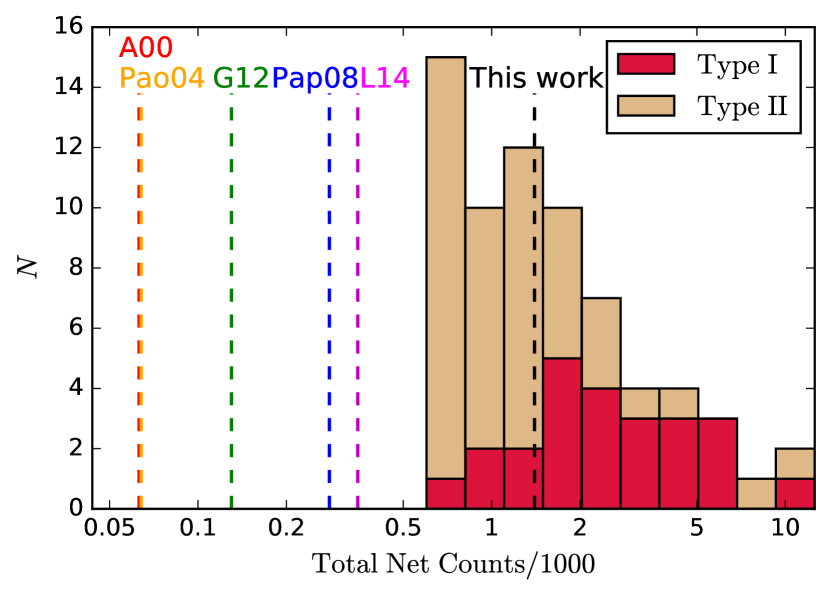
Sixty-eight sources are selected with 649–11283 counts; the median number of counts is 1399. Figure 2 shows the distribution of our counts. Our sources generally have more counts than those in previous studies, usually by substantial factors (Table 1), allowing improved source characterization. The faintest selected sources have fluxes (observed-frame 0.5–7 keV; see Section 3.2.2 for flux calculation) of $\approx 1\times 10^{-15}$ $\mathrm{erg\ cm^{-2}\ s^{-1}}$, similar to the full-band source-detection limit of the Chandra COSMOS-Legacy survey (e.g., Civano et al., 2016). We are thus characterizing in this work the AGNs responsible for producing much of cosmic accretion power; our measurements probe $\approx$ 20–3 times below the knee luminosity, $L_{\rm X}^{*}$, of the X-ray luminosity function at $z=0.5-4$ (e.g., Ueda et al., 2014; Aird et al., 2015).

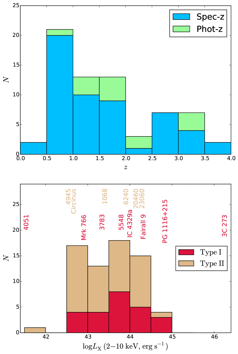
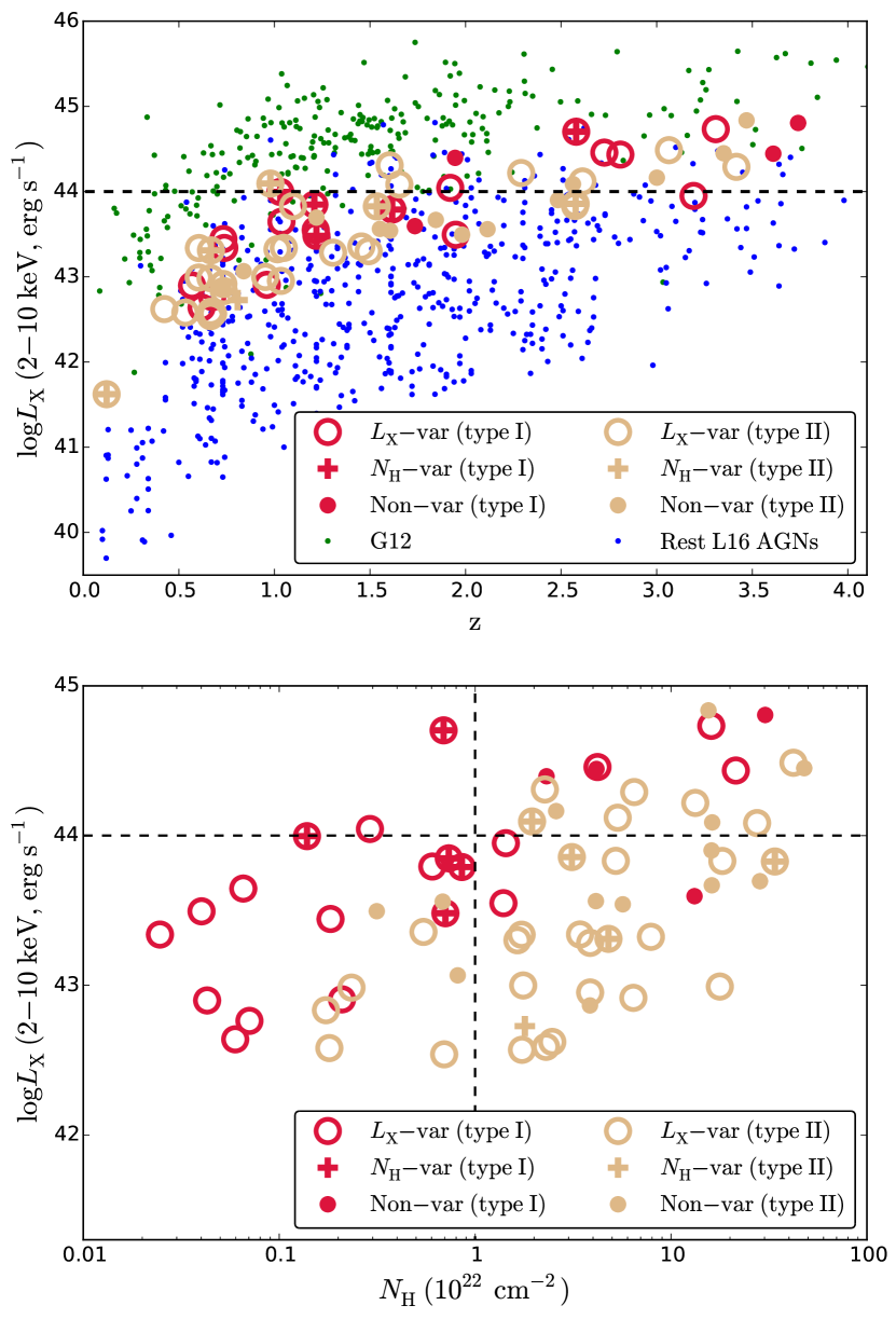
The spectroscopic and photometric redshift data are compiled by L16. For each source, we adopt the spectroscopic redshift (z_spec) either marked as “secure” by L16 or consistent with the photometric redshift (z_phot) measurement (i.e., z_phot differs from z_spec by less than 10%). Otherwise, if z_spec is not available or disagrees with z_phot, we adopt z_phot because “insecure” z_spec are less reliable than z_phot. Those insecure z_spec are often based on spectra with few features, e.g., a tentative single absorption line, but z_phot are derived from SED fitting of $\mathrel{\hbox to0.0pt{\lower 4.0pt\hbox{\hskip 1.0pt$\sim$}\hss}\raise 1.0pt\hbox{$>$}}15$ photometric bands (Luo et al., 2010; Hsu et al., 2014). In total, we have 55 z_spec and 13 z_phot. The z_phot quality is generally high (fractional errors $\sim$ a few percent) thanks to the wide multi-band photometric coverage used to derive z_phot (Luo et al., 2010; Hsu et al., 2014). The redshift and intrinsic X-ray luminosity $L_{\rm{X}}$ distributions of the sample are plotted in Figure 3, with the $L_{\rm{X}}$ values for some representative local AGNs marked for comparison purposes. The median $L_{\rm{X}}$ of our sources is $4\times 10^{43}\ \rm erg\ s^{-1}$, several times larger than that of the whole CDF-S AGN sample ($\approx 8\times 10^{42}\ \rm erg\ s^{-1}$, L16); the median redshifts of the two samples are similar ($\approx$1.5). Many local well-known AGNs have $L_{\rm{X}}$ within our luminosity coverage, and thus our sources, at least in this sense, appear to be distant analogs of these local AGNs.

We classify a source as type I if any broad emission line is reported in the redshift literature (20 sources); if only narrow emission lines/absorption lines are reported (35 sources) we assign a type II classification. We caution that there might be some intrinsic type I objects misclassified as type II due to, e.g., lack of spectral coverage of the hydrogen Balmer lines (e.g., Khachikian & Weedman, 1974) or the spectral S/N not being sufficient to identify broad lines. If the spectral classification of a source is not available in the literature, it is classified based on fitting of the spectral energy distribution (SED; data from Hsu et al., 2014): if its rest-frame optical color is blue (i.e., rest-frame $u-g<0.8$) we classify it as type I, otherwise as type II. This color-classification scheme results in 4 type I and 9 type II AGNs, in addition to the spectral classification. Therefore, our sample consists of 24 type I and 44 type II AGNs. The optical classification is broadly consistent with X-ray classification approaches (i.e., using the epoch-mean $N_{\rm{H}}$ $=10^{22}\rm\ cm^{-2}$ as the threshold for type II; see Section 3.2.1) despite some exceptions (see Figure 8). Type I sources generally have more counts than type II sources; their median counts are 2199 and 1098, respectively. Table 3 lists the properties of individual sources in our sample.

BAL quasars often show heavy and complex X-ray absorption despite their type I nature (e.g., Gallagher et al., 2002, 2006). It is of interest to investigate their X-ray variability behavior (e.g., Gallagher et al., 2004; Saez et al., 2012). There are 8 type I quasars in our sample, if we define quasars as AGNs with $L_{\rm{X}}$$>10^{44}\ \mathrm{erg\ s^{-1}}$. One of our objects has been reported as a BAL quasar (J033209.4–274806, e.g., Szokoly et al. 2004) at $z=2.81$; it is X-ray luminous ($L_{\rm{X}}$$\approx 3\times 10^{44}$ erg s^-1) and highly obscured ($N_{\rm{H}}$$\approx 2\times 10^{23}$ cm^-1) with an intrinsic power-law photon index $\Gamma=1.68$ (see Section 3.2). This small number of BAL quasars is expected considering only $\approx$20% of type I quasars are BAL quasars (e.g., Hewett & Foltz, 2003; Gibson et al., 2009).

Three of our sources, J033247.8–274232 at $z=0.98$, J033211.3–275213 at $z=3.74$, and J033212.9–275236 at $z=2.56$, are potentially detected in the NuSTAR hard band (8–24 keV; Mullaney et al. 2015). The matching between Chandra and NuSTAR sources was performed by Mullaney et al. (2015). J033247.8–274232 has an almost unambiguous NuSTAR counterpart, because it is the only bright Chandra source within $23^{\prime\prime}$ ($\approx 3$ times the typical NuSTAR positional uncertainty) of the NuSTAR source position. J033211.3–275213 and J033212.9–275236 are matched to a single NuSTAR source, and are both $\approx 15^{\prime\prime}$ from the NuSTAR counterpart. There are no other bright Chandra sources within $23^{\prime\prime}$ of this NuSTAR source position. Therefore, one of these two high-redshift Chandra sources likely has a NuSTAR hard-band detection.

Table 3Source Properties

Name (CXOCDFS)	RA	DEC	$z$	$\Delta z$	Opt. type	Off-Axis	Counts	$P_{\rm PF}$	$P_{\rm HR}$	$E_{peg}$	$goodness$	$\Gamma$
(1)	(2)	(3)	(4)	(5)	(6)	(7)	(8)	(9)	(10)	(11)	(12)	(13)
J033158.1–274833	52.99210	$-$27.80943	0.74	n/a	IIs	6.69	1366.0	0.00	32.75	0.50	10.2	1.52
J033158.2–275041	52.99283	$-$27.84490	3.31	0.09	Ic	7.05	2684.8	0.00	86.68	0.96	0.5	1.72
J033200.3–274319	53.00150	$-$27.72209	1.04	n/a	Is	7.96	3598.1	0.00	60.04	0.50	1.0	1.78
J033201.5–274327	53.00663	$-$27.72420	2.73	n/a	Is	7.67	2772.0	0.00	15.30	0.66	4.8	1.72
J033202.4–274600	53.01026	$-$27.76675	1.62	n/a	Is	6.18	2012.5	0.00	61.65	0.50	7.3	1.65

The full table contains 21 columns of information for 68 sources. (This table is available in its entirety in a machine-readable form in the online journal. A portion is shown here for guidance regarding its form and content.)
Column (1): Standard name of Chandra CDF-S sources.
Columns (2) and (3): J2000 coordinates.
Column (4): Adopted redshift. See L16 for redshift references.
Column (5): 1$\sigma$ errors of photometric redshift. n/a indicates a spectroscopic redshift has been used.
Column (6): Optical spectral type (see Section 2.2 for the classification scheme). Is (IIs): type I (II) from spectral classification; Ic (IIc): type I (II) from color classification. The spectral classifications are from Szokoly et al. (2004); Mignoli et al. (2005); Ravikumar et al. (2007); Tozzi et al. (2009); Treister et al. (2009); Silverman et al. (2010); Mao et al. (2012).
Column (7): Off-axis angle in units of arcminutes.
Column (8): Full-band (0.5–7 keV) total available net counts (not aperture corrected).
Columns (9) and (10): $p$-value of photon-flux and hardness-ratio variability, respectively (Section 3.1). Both are in units of %.
Column (11): The lower end of the normalization band used in $pegpwrlw$, in units of keV (Appendix A).
Column (12): $goodness$ of the spectral fitting ($wabs\times zwabs\times pegpwrlw$ model), in units of % (Section 3.2.1).
Column (13): Power-law photon index.
Columns (14) and (15): Epoch-mean values of intrinsic $L_{\rm{X}}$ (rest-frame 2–10 keV, in units of erg s^-1) and $N_{\rm{H}}$ (in units of cm^-2), respectively (Section 3.2.1).
Columns (16) and (17); Metrics ($\Delta$AIC_L and $\Delta$AIC_N) of the significance of $L_{\rm{X}}$ and $N_{\rm{H}}$ variability, respectively (Section 3.2.3).
Columns (18) and (19): Normalized excess variance of $L_{\rm{X}}$ variability (${\sigma^{2}_{\mathrm{exc},L}}$) and its uncertainty, respectively (Section 3.2.5).
Columns (20) and (21): Normalized excess variance of $N_{\rm{H}}$ variability (${\sigma^{2}_{\mathrm{exc},N}}$) and its uncertainty, respectively (Section 3.2.5). We only calculated this quantity for the 35 sources with all four epochs having $\delta N_{\mathrm{H},i}/N_{\mathrm{H},i}<0.4$ (see Appendix A); n/a indicates the other 33 sources.

Figure 2.— The histogram of total net counts of our 68 sources. The red and brown bars indicate type I and type II AGNs. The vertical dashed lines indicate the median counts of this work and previous studies, respectively (A00: Almaini et al. 2000; Pao04: Paolillo et al. 2004; Pap08: Papadakis et al. 2008; G12: Gibson & Brandt 2012, L14: Lanzuisi et al. 2014). Note that A00 and Pao04 have very similar median counts. We do not show the median counts of Shemmer et al. (2014) due to large fluctuations in counts among their seven sources. Our sample only includes bright sources with counts greater than 600. Our type I AGNs generally have more available counts than their type II counterparts.

Figure 3.— Upper panel: Redshift histogram for our 68 sources. The blue and green bars indicate sources with spectroscopic redshifts and photometric redshifts, respectively. Lower panel: Absorption-corrected X-ray luminosity (2–10 keV, rest-frame) histogram. The red and brown bars indicate type I and type II AGNs, respectively. The values are the epoch-mean $L_{\rm{X}}$ described in Section 3.2.1. Along the top of the panel, we label the typical absorption-corrected $L_{\rm{X}}$ values for some representative type I (red) and type II (brown) AGNs in the local universe. The 4-digit and 5-digit numbers indicate NGC and IRAS sources, respectively. The $L_{\rm{X}}$ data were compiled from the literature (e.g., Brandt et al., 1997; Ogasaka et al., 1997; Reynolds, 1997; George et al., 2000; Pounds et al., 2003; Arévalo et al., 2014; Puccetti et al., 2014, 2016; Bauer et al., 2015). Our sources cover wide ranges of both $z$ and $L_{\rm{X}}$. In terms of $L_{\rm{X}}$, our sources appear to be distant analogs of many local Seyfert galaxies and moderate-luminosity quasars.

3. Data Analyses

3.1. Photometric Variability

3.1.1 Method

We use full-band (0.5–7 keV) photometry to analyze photon-flux ($PF$, i.e., count rate per unit area, in units of counts s^-1 cm^-2) variability. For each epoch of a source, we calculate $PF$ as

$$PF_{i}=\frac{{net\_counts}_{i}}{{effarea}_{i}\times{exptime}_{i}},$$ (1)

and its uncertainty

$$\delta PF_{i}=\frac{{\delta net\_counts}_{i}}{{effarea}_{i}\times{exptime}_{i}},$$ (2)

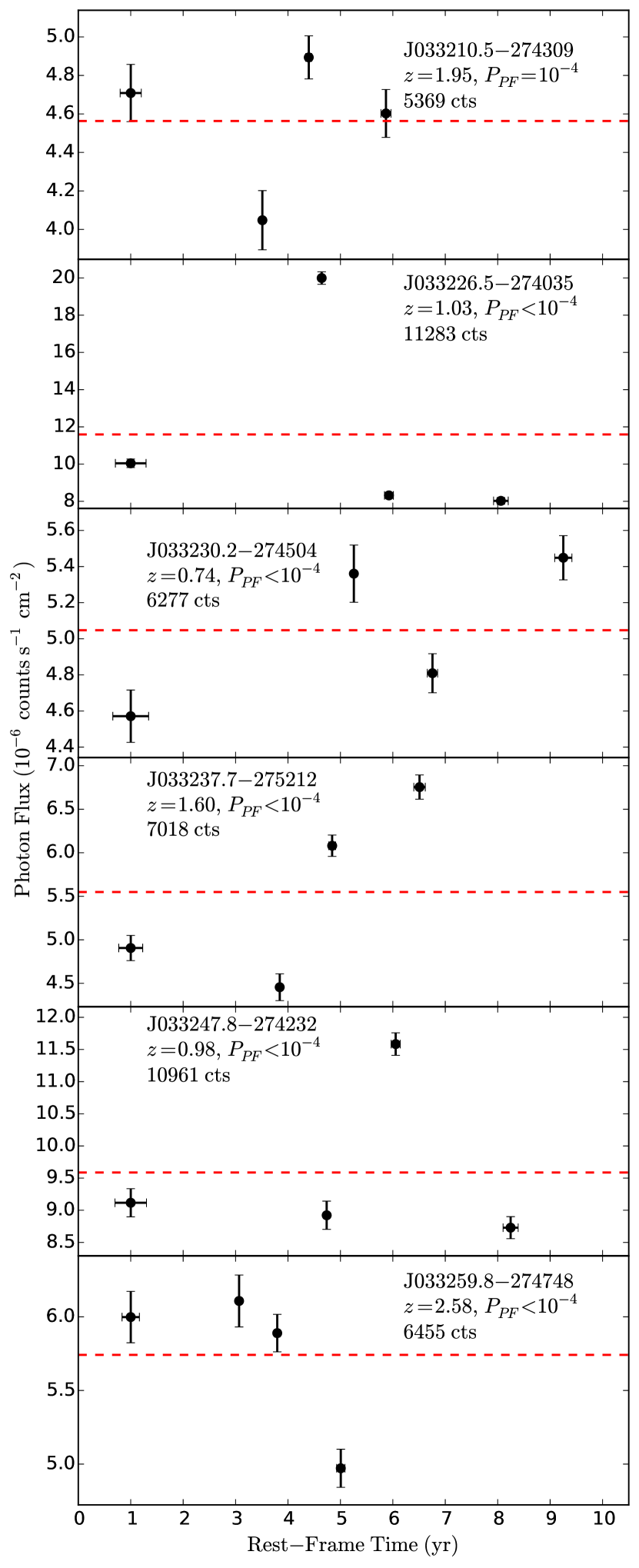
where the subscript $i$ denotes the epoch; ${net\_counts}_{i}$ and ${\delta net\_counts}_{i}$ are background-subtracted counts and corresponding error, respectively; $effarea_{i}$ and $exptime_{i}$ are the effective area and exposure time, respectively. The effective area is approximated as the average ancillary response file (ARF) weighted by the average CDF-S AGN spectrum (i.e., a $\Gamma=1.4$ power law with Galactic absorption; see, e.g., Paolillo et al., 2004). This procedure accounts for the varying sensitivity of Chandra among different epochs due to, e.g., quantum-efficiency degradation and gaps between CCDs, since these factors are considered by AE when calculating the ARF. Figure 4 shows light curves of the 6 sources with the most counts.

Figure 4.— Light curves of the 6 sources with the most counts. The red dashed horizontal lines indicate the unweighted mean of photon fluxes for each source. The horizontal error bars indicate the bin width of each epoch. The rest-frame time of epoch 1 is set to 1 yr. Some source properties are labeled on the corresponding panels. All of the 6 sources show photon-flux variability (i.e., $P_{PF}<5\%$).

To identify variable sources, we calculate the statistic

$$X^{2}_{PF}=\sum_{i=1}^{4}\frac{(PF_{i}-\langle PF\rangle)^{2}}{(\delta PF_{i})^{2}},$$ (3)

where $\langle PF\rangle$ is the unweighted mean of $PF_{i}$ (e.g., Turner et al., 1999). For sources with large numbers of counts, the probability distribution of $PF$ approaches the normal distribution, and thus $X^{2}_{PF}$ should follow the $\chi^{2}$ distribution with three degrees of freedom ($\chi^{2}_{\rm dof=3}$). Our sources have at least 600 total net counts (at least $\sim 150$ counts or $\mathrm{S/N}\sim 12$ per bin). Therefore $\chi^{2}_{\rm dof=3}$ should be a good approximation of $X^{2}_{PF}$. To verify this point and find an accurate $p$-value ($P_{PF}$) from $X^{2}_{PF}$, we adopt a Monte Carlo simulation strategy similar to that in Paolillo et al. (2004) and Young et al. (2012). The null hypothesis is that $PF$ remains constant in the four epochs at $PF_{\mathrm{mean}}$. To perform the simulations, we need to know model counts in each epoch. We convert $PF_{\mathrm{mean}}$ to the net counts expected in each epoch as

$$net\_counts_{i}^{\mathrm{model}}=PF_{\mathrm{mean}}\times{effarea}_{i}\times exptime_{i}.$$ (4)

We obtain the model source counts (not background subtracted) and model background counts as

$$\begin{gathered}{src\_counts}_{i}^{\mathrm{model}}={net\_counts}_{i}^{\mathrm{model}}+\frac{{bkg\_counts}_{i}^{\mathrm{observed}}}{backscal_{i}},\\ {bkg\_counts}_{i}^{\mathrm{model}}={bkg\_counts}_{i}^{\mathrm{observed}},\end{gathered}$$ (5)

where $backscal$ is the factor produced by AE that scales background counts (usually obtained in a large aperture) to the source-extraction aperture. We use ${src\_counts}_{i}^{\mathrm{model}}$ (${bkg\_counts}_{i}^{\mathrm{model}}$) as the mean in a Poisson distribution to simulate ${src\_counts}_{i}$ (${bkg\_counts}_{i}$), and extract photometry following the algorithm in AE. We obtain the $X^{2}_{PF}$ for a simulated data set (10000 simulations) following the same procedures as described above. We perform Kolmogorov-–Smirnov (KS) tests between the simulated $X^{2}_{PF}$ distributions and the $\chi^{2}_{\rm dof=3}$ distribution. The resulting KS statistics for our sources have median 0.015; this small value indicates our simulated $X^{2}_{PF}$ distributions are very similar to the $\chi^{2}_{\rm dof=3}$ distribution.

We define the hardness ratio ($HR$) for a source in an epoch as

$$HR_{i}=\frac{PF_{i,hard}-PF_{i,soft}}{PF_{i,hard}+PF_{i,soft}},$$ (6)

where $PF_{i,hard}$ and $PF_{i,soft}$ are photon fluxes as defined above but for the hard band (2–7 keV) and soft band (0.5–2 keV), respectively. We estimate the error of $HR$ from error propagation as

$$\begin{gathered}\delta HR_{i}=\frac{2PF_{i,hard}PF_{i,soft}}{(PF_{i,hard}+PF_{i,soft})^{2}}\times\\ \sqrt{\left(\frac{\delta PF_{i,hard}}{PF_{i,hard}}\right)^{2}+\left(\frac{\delta PF_{i,soft}}{PF_{i,soft}}\right)^{2}}.\end{gathered}$$ (7)

To identify $HR$-variable sources, we calculate

$$X^{2}_{HR}=\sum_{i=1}^{4}\frac{(HR_{i}-\langle HR\rangle)^{2}}{(\delta HR_{i})^{2}},$$ (8)

where $\langle HR\rangle$ is the unweighted mean of $HR_{i}$.

We perform similar simulations as above to convert $X^{2}_{HR}$ to a $p$-value ($P_{HR}$). The null-hypothesis is that $HR_{i}$ is constant and equals $HR_{\mathrm{mean}}$ over the four epochs. We approximate the model full-band net counts as the sum of the observed hard-band and soft-band net counts,

$${net\_} {counts}_{i,full}^{\mathrm{model}}=$$ (9)

$${net\_counts}_{i,hard}^{\mathrm{observed}}+{net\_counts}_{i,soft}^{\mathrm{observed}}.$$

The model hard-band and soft-band net counts are calculated by

$${net\_} {counts}_{i,hard}^{\mathrm{model}}=$$ (10)

$${net\_counts}_{i,full}^{\mathrm{model}}\times$$

$$(\frac{{net\_counts}_{i,hard}}{{net\_counts}_{i,hard}+{net\_counts}_{i,soft}})^{\mathrm{model}}$$

$$= {net\_counts}_{i,full}^{\mathrm{model}}\times$$

$$\frac{1}{2}(1+(\frac{{net\_counts}_{i,hard}-{net\_counts}_{i,hard}}{{net\_counts}_{i,hard}+{net\_counts}_{i,soft}})^{\mathrm{model}})$$

$$= {net\_counts}_{i,full}^{\mathrm{model}}\times\frac{1+HR_{\mathrm{mean}}}{2}$$

and

$${net\_} {counts}_{i,soft}^{\mathrm{model}}=$$ (11)

$${net\_counts}_{i,full}^{\mathrm{model}}-{net\_counts}_{i,hard}^{\mathrm{model}},$$

respectively.

Knowing ${net\_counts}_{i,hard(soft)}^{\mathrm{model}}$, we obtain ${src\_counts}_{i,hard(soft)}^{\mathrm{model}}$ and ${bkg\_counts}_{i,hard(soft)}^{\mathrm{model}}$ using Equation 5. Similar to the case of $X^{2}_{PF}$, the simulated $X^{2}_{HR}$ distributions are close to the $\chi^{2}_{\rm dof=3}$ distribution. The KS statistics derived from comparing simulated $X^{2}_{HR}$ distributions and $\chi^{2}_{\rm dof=3}$ have median 0.023.

3.1.2 Results

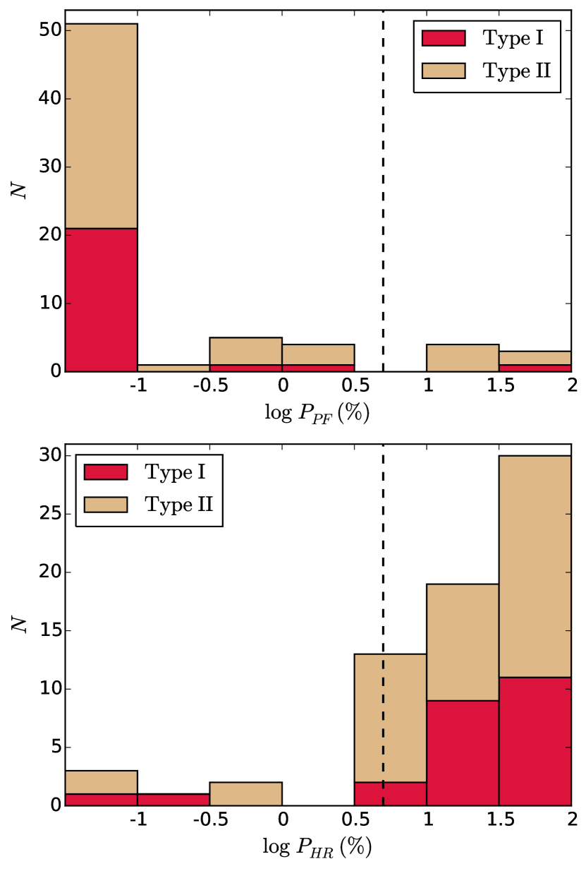
The histograms of $P_{PF}$ and $P_{HR}$ are presented in Figure 5. Using $P=5\%$ as the threshold for variability ($\sim 68\times 5\%\mathrel{\hbox to0.0pt{\lower 4.0pt\hbox{\hskip 1.0pt$\sim$}\hss}\raise 1.0pt\hbox{$<$}}4$ false positives expected), 90% (61/68) and 16% (11/68) of our sources display $PF$ variability and $HR$ variability, respectively. All of our six sources with the most counts are variable (see Figure 4). Changing the threshold to $P=1\%$ ($\sim 68\times 1\%\mathrel{\hbox to0.0pt{\lower 4.0pt\hbox{\hskip 1.0pt$\sim$}\hss}\raise 1.0pt\hbox{$<$}}1$ false positive expected) leads to a $PF$-variable fraction and a $HR$-variable fraction of 84% (57/68) and 9% (6/68), respectively. This $PF$-variable fraction (84%) is higher than that of optically selected Sloan Digital Sky Survey (SDSS, York et al. 2000) quasars under the same confidence level (i.e., 65%; the sample is from G12 with the same count constraint of 600 applied). This result supports an intrinsic anticorrelation between variability amplitude and X-ray luminosity (see Section 3.2.6), considering those SDSS quasars are generally $\approx 10$ times more X-ray luminous than our sources (see Table 1 and Section 3.2.3). However, this behavior might also be a result of different rest-frame time samplings (see Figure 1). With the $P=5\%$ threshold, almost all (23/24) type I AGNs and 86% (38/44) of type II AGNs are $PF$ variable; 13% (3/24) of type I AGNs and 18% (8/44) of type II AGNs are $HR$ variable. The higher $PF$-variable source fraction for type I sources might be due to their higher numbers of counts (Figure 2). Type II sources are more likely to be $HR$ variable despite their smaller numbers of counts However, Fisher’s exact test shows that the dependences of variable source fractions on optical spectral type are not statistically significant.

Figure 5.— The histograms of $P_{PF}$ (upper panel) and $P_{HR}$ (lower panel). The red and brown bars indicate type I and type II AGNs, respectively. The vertical black dashed lines in both panels indicate the value of 5%, our variability criterion. The leftmost column indicates all sources with $P_{PF}$ ($P_{HR}$) $<0.1\%$. Photon-flux variability is generally more common than hardness-ratio variability.

3.1.3 Variability Within Each Epoch

We also use each Chandra observation as a bin to analyze the variability within each epoch ($\mathrel{\hbox to0.0pt{\lower 4.0pt\hbox{\hskip 1.0pt$\sim$}\hss}\raise 1.0pt\hbox{$<$}}1$ yr, observed-frame). The observation lengths range from about 30 to 100 ks (see L16). We calculate $P_{PF}$ and $P_{HR}$ for each source within each of the four epochs. The method is the same as described in Section 3.1.1. $PF$ variability is still significant: the $PF$-variable (i.e., $P_{PF}<5\%$) source fractions are 49%, 29%, 56%, and 38% for each bin, respectively. We find the variable source fraction is higher for sources with more counts, likely due to their higher S/N. We do not detect statistically significant $HR$ variability: the $HR$-variable (i.e., $P_{HR}<5\%$) source fractions are 3%, 3%, 1%, and 3%, respectively, consistent with the expected false-positive rate. This result is likely due to the low S/N in this dataset compared to that of the binned data.

More detailed analyses based on such a binning strategy will be presented in another paper (X. C. Zheng et al., in preparation). Those analyses suggest that short-term (days-to-months) variability of our sources by large amplitudes (e.g., more than a factor of two) is rare, similar to our results on long time scales (Sections 3.2.2 and 3.2.5).

3.2. Spectral Variability

3.2.1 Method

The photometric analyses in Section 3.1 roughly evaluate the spectral normalization and shape changes. To characterize the spectral variability more accurately as well as gain improved physical insights, we perform spectral fitting for each source. The fitting is based on full-band (observed-frame 0.5–7 keV) spectra to maximize the available counts. Given our high-quality X-ray spectra (with a median full-band S/N $\approx 17$ in each epoch) owing to the good angular resolution and low source-cell background of Chandra, we can still do reliable spectral fitting even though the counts per epoch (median $\sim 350$) are moderate. Note that we are typically accessing penetrating rest-frame X-rays up to $\approx 10-30$ keV.

We use XSPEC v12.9.0i (Arnaud, 1996) to carry out spectral fitting. Counts are not binned over different ACIS pulse height amplitude (PHA) channels, and the Cash statistic (Cash, 1979) is used for fitting. Considering the available counts, we adopt a simple fitting model of a power law with Galactic and intrinsic absorption $wabs\times zwabs\times pegpwrlw$ (see Morrison & McCammon 1983 for the $wabs$ and $zwabs$ models). We adopt $pegpwrlw$ (normalized over a finite energy band) instead of the widely used $powerlaw$ (normalized at observed-frame 1 keV) for the reasons described in Appendix A. We fix the redshift ($zwabs$) as the adopted value in Section 2.2. The allowed ranges of $N_{\rm{H}}$ ($zwabs$) and $\Gamma$ ($pegpwrlw$) are set to $10^{19}-10^{24}\ \rm cm^{-2}$ and $1.2-2.4$, respectively. The counts of our sources in each epoch (median $\sim 350$) generally cannot constrain $\Gamma$ effectively; e.g., Brightman et al. (2013) found that even a simple $powerlaw$ model would require $\mathrel{\hbox to0.0pt{\lower 4.0pt\hbox{\hskip 1.0pt$\sim$}\hss}\raise 1.0pt\hbox{$>$}}1000$ counts to obtain an uncertainty (90% confidence level) of $\Gamma$ within 0.2. Studies of quasars and local luminous AGNs show that spectral variability generally follows a “softer when brighter” behavior (e.g., Sobolewska & Papadakis, 2009; Gibson & Brandt, 2012; Sarma et al., 2015; Connolly et al., 2016). However, based on the empirical X-ray flux–$\Gamma$ relations given by those studies, the $\Gamma$ variability amplitudes for our sources are expected to be small and not detectable given the counts we have in each epoch. For example, flux variability by a factor of two (about the upper limit of our flux-variability amplitudes; see Section 3.2.2) only produces $\Delta\Gamma\approx 0.1$. Motivated by this expected near constancy of $\Gamma$, we thus simultaneously fit the spectra of all four epochs by linking their photon indexes $\Gamma$ ($pegpwrlw$), assuming no substantial $\Gamma$ variability. Considering the low source-cell backgrounds and high count numbers for our sources, we do not specifically model the background but employ the XSPEC default background modeling strategy. The $norm_{i}$ (i.e., normalization of $pegpwrlw$) and $N_{\rm{H}}$_,i ($zwabs$) are set free and not linked across epochs, where subscripts $i$ denote the epoch indexes. This spectral fitting yields best-fit model parameters, i.e., $\Gamma_{\mathrm{fit}}$, $norm_{i}$, and $N_{\rm{H}}$_,i, and the errors of $norm_{i}$. The errors of $N_{\rm{H}}$_,i are estimated with the method detailed in Appendix A. This method is critical for obtaining accurate errors of $N_{\rm{H}}$_,i for the reasons explained in Appendix A. The $\Gamma_{\mathrm{fit}}$ distribution is shown in Figure 6. The distribution is similar to that found by Tozzi et al. (2006), except that our dispersion is smaller likely due to our larger numbers of counts. We set both Galactic and intrinsic absorption to none and calculate the absorption-corrected X-ray luminosity in the rest-frame 2–10 keV band for each epoch. The unweighted-mean luminosity (absorption column density) of the four epochs is denoted as $L_{\rm{X}}$ ($N_{\rm{H}}$) and widely used throughout this paper.

Figure 6.— Upper panel: best-fit $\Gamma$ histogram. Lower panel: $goodness$ histogram. The $goodness$ distribution indicates the $wabs\times zwabs\times pegpwrlw$ model generally describes our data acceptably.

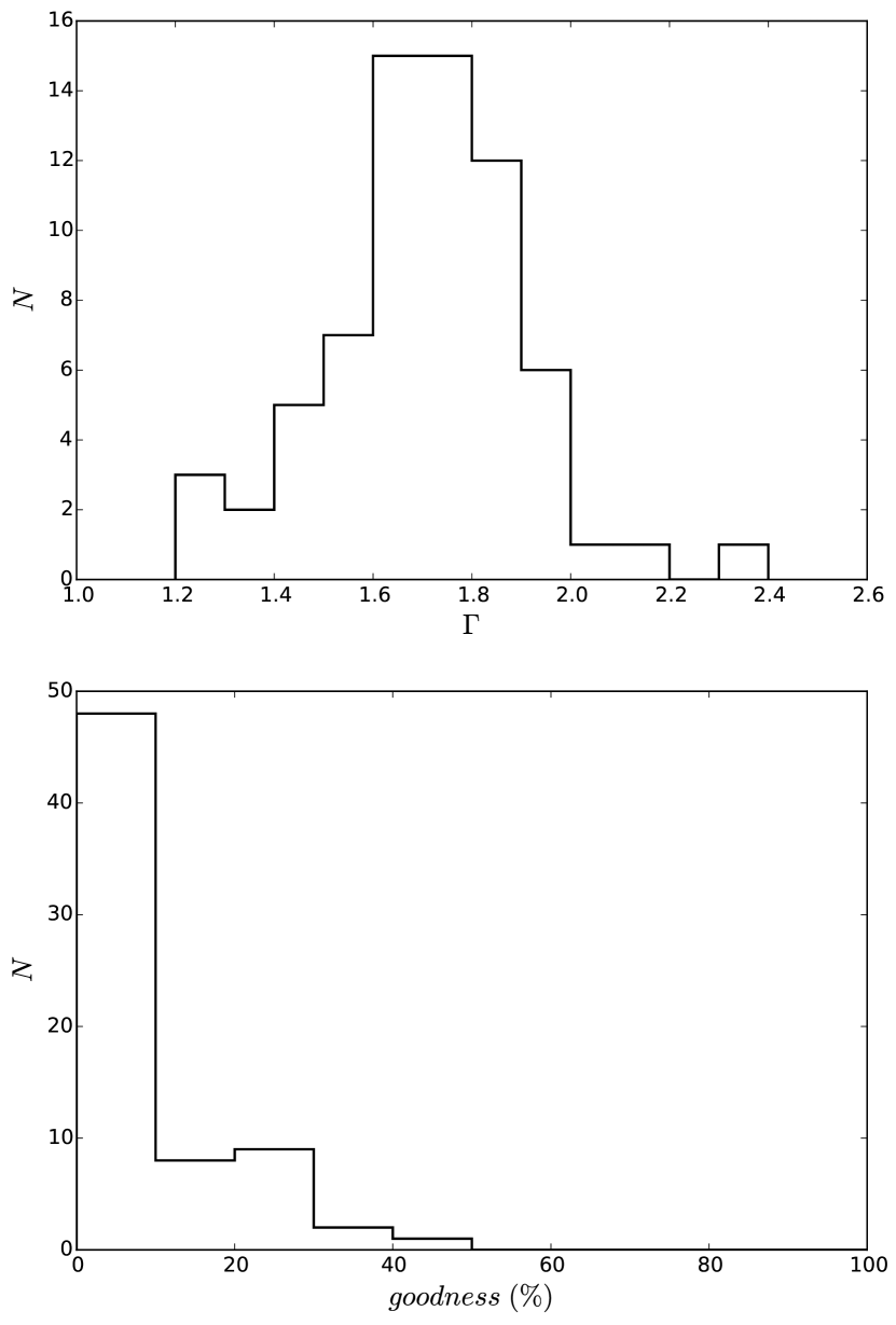
Since we fit the unbinned spectra with the Cash statistic, the spectral-fit quality cannot be inferred directly from the best-fit statistic, e.g., $\chi^{2}/\rm dof$ in the minimum $\chi^{2}$ fitting case. Instead, we perform goodness-of-fit Monte Carlo simulations for each source in XSPEC. XSPEC simulates 1000 spectra from the best-fit parameters, and calculates the fraction ($goodness$) of simulated spectra with KS statistic less than that of the observed spectrum. Here, the KS statistic is used to describe the “similarity” between a spectrum and the model, similar to $\chi^{2}$ in the minimum $\chi^{2}$ fitting case. In other words, $goodness$ can be interpreted as the confidence level to reject the model. The distribution of $goodness$ is presented in Figure 6. The fits are acceptable ($goodness<50\%$, e.g., Corral et al. 2015) for all our sources. The worst case is J033218.3–275055 with $goodness=44\%$, a Compton-thick candidate reported in the literature (Tozzi et al., 2006; Comastri et al., 2011). A detailed discussion of this source is presented in Appendix B.

3.2.2 Flux Variability over 15 Years

Long-term X-ray variability may affect physical inferences about X-ray source populations; e.g., the star-formation vs. AGN-activity connection may be affected by $\sim$Myr timescale AGN variability (e.g., Hickox et al. 2014). It is thus of interest to assess whether X-ray variability on the longest observable time scales (i.e., between epoch 1 and epoch 4) substantially affects the appearance of the overall X-ray source population.

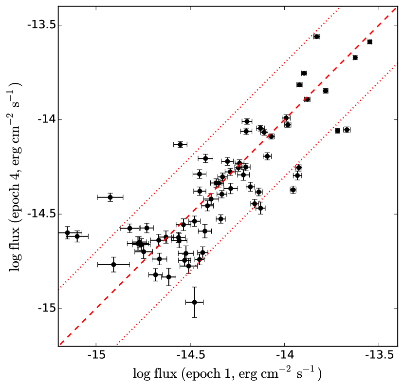
Figure 7 displays the full-band fluxes of epoch 1 and epoch 4. Applying Spearman’s test on the fluxes of epoch 1 and epoch 4 yields $\rho=0.82$ and a $p$-value of $10^{-17}$; the large value of $\rho$ indicates a good association of ranks. In general, the brightest (faintest) sources remain the brightest (faintest) after 15 years. Only 11 ($11/68=16\%$) sources have flux changes greater than a factor of two. Qualitatively similar results are obtained when we pair any two of our available epochs.

The rarity of extremely variable sources in the distant universe over long time scales is broadly consistent with a recent study focusing on low-redshift AGNs (Strotjohann et al., 2016). Our results prove that, at least on a 15-year observed-frame time scale, basic inferences about distant AGN source populations are not strongly affected by variability, e.g., the expected star-formation vs. AGN-activity connection is unlikely to be hidden by AGN variability on a rest-frame time scale of $\sim 5-10$ years. These results also show that X-ray changing-look AGNs are rare, and they constrain the frequency of other types of novel long-term X-ray variability (see Section 1). Setting direct X-ray constraints on much longer time scales is unfortunately limited by, e.g., the age of X-ray astronomy. Cosmic X-ray surveys often bin observations performed over 1–15 years; our results indicate that long-term variability is not likely to affect the interpretation of such survey results greatly.

Figure 7.— Flux (epoch 4) vs. flux (epoch 1). The fluxes are calculated from our spectral-fitting results (see Section 3.2.1), and are not corrected for Galactic or intrinsic absorption. The energy band is observed-frame 0.5–7 keV (i.e., full-band). The red dashed line indicates no flux change; the red dotted lines indicate flux changes by a factor of 2. The ranks of fluxes are similar in the two epochs. Thus, X-ray variability over 15 years does not significantly affect the appearance of the overall X-ray source population.

3.2.3 Identification of $L_{\rm{X}}$- and $N_{\rm{H}}$- Variable Sources

We identify $L_{\rm{X}}$- and $N_{\rm{H}}$-variable sources using the Akaike information criterion (AIC, Akaike, 1974). The AIC is based on information theory and does not assume a particular model-fitting technique or distribution of uncertainties (e.g., Burnham & Anderson, 2002; Kelly et al., 2007; Buchner et al., 2014). AIC is defined as $\mathrm{AIC}=C+2k$, where $C$ is the fitting statistic (i.e., the Cash statistic in our case) and $k$ is the number of free parameters in the model. Models with smaller AIC are considered to be more probable.

For each source, we calculate AIC (denoted as $\rm{AIC_{0}}$) for the spectral-fitting results in Section 3.2.1. To evaluate the significance of $L_{\rm{X}}$ variability, we link $norm_{i}$ in all spectra of the four epochs, and redo the fitting. Other settings of the model are the same as in Section 3.2.1. We calculate AIC for the new fitting results, denoted as AIC₁. We use the difference $\Delta\mathrm{AIC}_{L}=\rm AIC_{1}-AIC_{0}$ to evaluate the significance of $L_{\rm{X}}$ variability. If $\Delta\mathrm{AIC}_{L}>4$ (e.g., Burnham & Anderson, 2002), we assign this source as an $L_{\rm{X}}$-variable source. Similarly, we identify $N_{\rm{H}}$-variable sources by calculating the AIC difference $\Delta$AIC_N between $N_{\rm{H}}$-linked and unlinked models and comparing it with the threshold of 4. The $\Delta\mathrm{AIC}_{L}$ and $\Delta\mathrm{AIC}_{N}$ for each source are listed in Table 3.

The resulting $L_{\rm{X}}$- and $N_{\rm{H}}$-variable source fractions are 74% (50/68) and 16% (11/68), respectively. Four of the 11 $N_{\rm{H}}$-variable sources are $HR$-variable (Section 3.1). The other 7 sources have large $P_{HR}$ values ($>10\%$). One reason for this result is likely to be that the definition of HR (Equation 6) uses observed-frame 2 keV as the boundary between the soft and hard bands. This choice of 2 keV is just by convention. It corresponds to different rest-frame energies for different sources and might not be sensitive in selecting some $N_{\rm{H}}$-variable sources. We checked the 4-epoch spectra of the 7 sources, and found that 2 keV as a boundary is either too high or too low to detect their $N_{\rm{H}}$ variability effectively.

Most (10/11) $N_{\rm{H}}$ variable sources are also $L_{\rm{X}}$ variable. The median $\Delta\mathrm{AIC}_{L}$ ($\Delta\mathrm{AIC}_{N}$) for $L_{\rm{X}}$-variable ($N_{\rm{H}}$-variable) sources is 43 (6.2). Therefore, our $L_{\rm{X}}$ variability is generally more significant than $N_{\rm{H}}$ variability. The BAL quasar J033209.4–274806 shows $L_{\rm{X}}$ variability ($\Delta$AIC${}_{L}=4.9$) but not $N_{\rm{H}}$ variability ($\Delta$AIC${}_{N}=-2.7$). We investigate three significantly variable sources, J033226.5–274035, J033259.7–274626, and J033229.9–274530, as illustrative examples in Appendix C. Notably, J033229.9–274530 transitions from an X-ray unobscured to obscured state. The positions of the identified variable sources in the $L_{\rm{X}}$-$z$ and $L_{\rm{X}}$-$N_{\rm{H}}$ planes are indicated in Figure 8. G12 performed similar variability analyses but for optically selected SDSS quasars. Their quasars are included in the $L_{\rm{X}}$-$z$ plot to demonstrate the differences between their sample and ours. Luminosities for the G12 objects are estimated assuming a power law with $\Gamma=1.8$. The typical luminosity of our sources is generally about one order of magnitude lower than that of the SDSS quasars at a given redshift. The majority ($\approx 60\%$) of the X-ray obscured quasars (i.e., $N_{\rm{H}}$$>10^{22}\ \mathrm{cm^{-2}}$ and $L_{\rm{X}}$$>10^{44}$ erg s^-1) in our sample are $L_{\rm{X}}$-variable, supporting the idea that we are observing their central X-ray emitting regions directly. Also, 7 of our 11 optically classified type II quasars show $L_{\rm{X}}$ variability (Figure 8). The well-studied optically classified type II quasar at $z=3.70$ in the CDF-S (e.g., Norman et al., 2002; Comastri et al., 2011) is not included in our sample due to its limited number of available counts (see Section 2.2).

Figure 8.— Upper panel: $L_{\rm{X}}$ vs. $z$. The open circles, crosses and solid circles indicate $L_{\rm{X}}$-variable, $N_{\rm{H}}$-variable, and non-variable sources, respectively. A source can be both $L_{\rm{X}}$-variable and $N_{\rm{H}}$-variable. Red and brown colors indicate type I and type II sources, respectively. The green and the blue points indicate G12 quasars and the rest of the AGNs in L16. At a given redshift, our sources are generally less luminous than G12 quasars and more luminous than the other L16 AGNs. The dashed horizontal line indicates our definition of quasars (i.e., $L_{\rm{X}}$$>10^{44}\ \mathrm{erg\ s^{-1}}$, see Section 2.2). Lower panel: $L_{\rm{X}}$ vs. $N_{\rm{H}}$. The symbols have the same meanings as for the upper panel. The horizontal and vertical dashed lines indicate our definition of quasars and the common definition of X-ray obscured AGNs (i.e., $N_{\rm{H}}$$>10^{22}\ \mathrm{cm^{-2}}$), respectively.

3.2.4 Relation Between $L_{\rm{X}}$ and $N_{\rm{H}}$ Variability

If the observed $N_{\rm{H}}$ variability were caused by changes of the ionization parameter of the obscuring matter, an anticorrelation between $L_{\rm{X}}$ and $N_{\rm{H}}$ variability might be expected; when $L_{\rm{X}}$ rises, the obscuring matter would become more ionized and generally less opaque. We performed a Spearman’s test on $L_{\mathrm{X},i}/L_{\mathrm{X}}$ and $N_{\mathrm{H},i}/N_{\mathrm{H}}$ for the 10 sources together that show both $L_{\rm{X}}$ and $N_{\rm{H}}$ variability, but do not find a significant anticorrelation. There is also no significant anticorrelation produced if we expand the Spearman’s test to all sources. Therefore, the $N_{\rm{H}}$ variability is not likely to be primarily driven by changes of ionization parameter. Nevertheless, some ionization-driven $N_{\rm{H}}$ variability might still exist if there are year-scale time delays between $L_{\rm{X}}$ and $N_{\rm{H}}$ variability due to, e.g., a low density of the absorber (e.g., Krolik & Kriss, 1995; Collinge et al., 2001).

3.2.5 Variability Amplitude Estimation

In this section, we illustrate and evaluate our method to quantify variability amplitude, and the results are used in all subsequent material. We use the normalized excess variance (${\sigma^{2}_{\rm exc}}$, e.g., Turner et al. 1999; Vaughan et al. 2003) to estimate intrinsic variability scale for $L_{\rm{X}}$ ($N_{\rm{H}}$) of each source. ${\sigma^{2}_{\rm exc}}$ is calculated as

$$\sigma_{\rm exc}^{2}=\frac{1}{N\langle x\rangle^{2}}\sum_{i=1}^{N}[(x_{i}-\langle x\rangle)^{2}-(\delta x_{i})^{2}],$$ (12)

where $N$ is the number of epochs (i.e., 4); $x_{i}$ and $\delta x_{i}$ are the best-fit $norm_{i}$ ($N_{\rm{H}}$_,i) and its 1$\sigma$ error $\delta norm_{i}$ ($\delta N_{\mathrm{H},i}$), respectively; $\langle x\rangle$ is the unweighted mean of $norm_{i}$ ($N_{\rm{H}}$_,i). The error of ${\sigma^{2}_{\rm exc}}$ is estimated as $s_{D}/(\langle x\rangle^{2}\sqrt{N})$, where

$$s^{2}_{D}=\frac{1}{N-1}\sum_{i=1}^{N}[(x_{i}-\langle x\rangle)^{2}-(\delta x_{i})^{2}-\sigma^{2}_{\rm exc}\langle x\rangle^{2}]^{2}.$$ (13)

is the variance of the summed terms $(x_{i}-\langle x\rangle)^{2}-(\delta x_{i})^{2}$ in Equation 12. We calculate the $L_{\rm{X}}$ ${\sigma^{2}_{\rm exc}}$ (${\sigma^{2}_{\mathrm{exc},L}}$) for each source. We only derive the $N_{\rm{H}}$ ${\sigma^{2}_{\rm exc}}$ (${\sigma^{2}_{\mathrm{exc},N}}$) for the 35 sources with all four epochs having $N_{\rm{H}}$_,i fractional errors $\delta N_{\mathrm{H},i}/N_{\mathrm{H},i}<0.4$ (Appendix A).

The results are listed in Table 3. While ${\sigma^{2}_{\mathrm{exc},L}}$ and ${\sigma^{2}_{\mathrm{exc},N}}$ are designed to measure intrinsic variability under ideal conditions, they may also be affected by the available counts (e.g., Allevato et al., 2013). However, the biases are minimized for high S/N, as is the case for our data (Section 3.2.1). Indeed, Spearman’s test demonstrates no significant dependence of ${\sigma^{2}_{\mathrm{exc},L}}$ and ${\sigma^{2}_{\mathrm{exc},N}}$ on the number of counts.

3.2.6 Variability Dependence on Luminosity, X-ray Absorption, and Redshift

It has been well established that the strength of AGN X-ray flux variability decreases as luminosity increases on time scales from minutes to about a year (e.g., Paolillo et al., 2004; Ponti et al., 2012). Also, studies of local Seyfert galaxies show that more obscured sources tend to be less variable on short time scales (minutes to hours; e.g., Turner et al., 1997; Hernández-García et al., 2015). Therefore, it is of interest to investigate the dependence of long-term (years) variability on luminosity and absorption level. Figure 9 shows the dependence of ${\sigma^{2}_{\mathrm{exc},L}}$ on $L_{\rm{X}}$. The unweighted mean of ${\sigma^{2}_{\mathrm{exc},L}}$ decreases toward higher luminosity. For each bin, the error on the mean is calculated as the standard deviation of individual ${\sigma^{2}_{\mathrm{exc},L}}$ divided by $\sqrt{N}$, where $N$ is the number of sources in the bin [i.e., Equation 13 of Allevato et al. (2013); but note that a power index of 2 is missing in their summed term]. The mean value in each bin can well represent the typical variability amplitude of the sources in the bin, despite the large error bars for individual sources (e.g., Allevato et al., 2013); the median has not been established to represent the typical variability amplitude. Spearman’s test applied to the individual sources shows a significant anticorrelation between ${\sigma^{2}_{\mathrm{exc},L}}$ and $L_{\rm{X}}$ (Spearman’s $\rho=-0.31$, $p$-value$=0.009$). This anticorrelation is mainly caused by the ${\sigma^{2}_{\mathrm{exc},L}}$ difference between quasars ($L_{\rm{X}}$$>10^{44}$ erg s^-1) and other AGNs. After removing quasars (only 19 sources), we find no significant relation between $L_{\rm{X}}$ and ${\sigma^{2}_{\mathrm{exc},L}}$. There is also tentative evidence of an anticorrelation between ${\sigma^{2}_{\mathrm{exc},L}}$ and $N_{\rm{H}}$: Spearman’s $\rho=-0.23$, $p$-value$=0.06$. However, this result might be a byproduct of the ${\sigma^{2}_{\mathrm{exc},L}}$-$L_{\rm{X}}$ relation, since in our counts-limited sample (i.e., $>600$ net counts required) heavily obscured sources tend to be more luminous compared to less-obscured sources (see Figure 8). This interpretation is supported by the fact that no significant ${\sigma^{2}_{\mathrm{exc},L}}$-$N_{\rm{H}}$ relation is found for luminosity-controlled samples ($L_{\rm{X}}$$\leq 10^{44}\ \mathrm{erg\ s^{-1}}$ and $L_{\rm{X}}$$>10^{44}\ \mathrm{erg\ s^{-1}}$).

Figure 9.— ${\sigma^{2}_{\mathrm{exc},L}}$ vs. $L_{\rm{X}}$. $L_{\rm{X}}$ values are the mean values in Section 3.2.1. Gray points indicate each individual source. The red squares indicate the mean value of each bin. The red horizontal error bars indicate the bin widths; the red vertical error bars indicate the errors on the mean values calculated analytically (see Section 3.2.6). The green shaded region indicates the ${\sigma^{2}_{\mathrm{exc},L}}$ expected from a power-law PSD with a slope of $-1$ (see Section 4.2). Our ${\sigma^{2}_{\mathrm{exc},L}}$ decreases at high luminosity. This is likely caused by the fact that our highest sampling frequency exceeds the PSD break frequency of the luminous sources (Section 4.2).

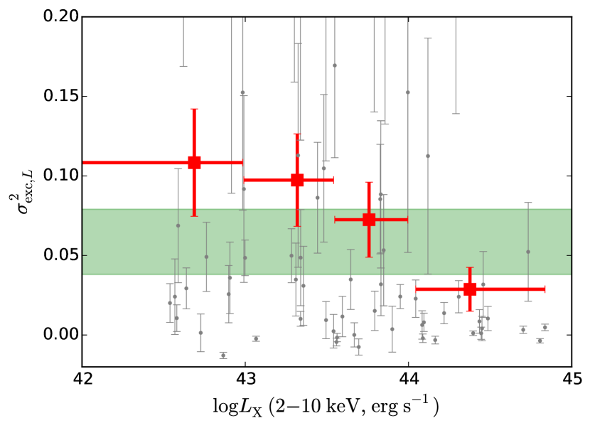
The anticorrelation between ${\sigma^{2}_{\mathrm{exc},L}}$ and $L_{\rm{X}}$ is unlikely to be a bias caused by the available counts, since we are in a high S/N regime (see Section 3.2.5). Another bias might exist considering that we are probing generally shorter time scales for more luminous sources, since they have relatively high redshifts (see Figure 8), increasing the effects of time-dilation. To test this point, we drop the first-epoch data for the low-redshift sample ($z<2$, median $z=1.0$), while keeping all data for the high-redshift sample ($z\geqslant 2$, median $z=2.8$). Hence, the observed-frame total time spans are about 8 and 15 years for the low- and high-redshift samples, respectively (see Table 2). The median values of the rest-frame total time spans are both about 4 years [low-redshift: 8/(1+1.0), high-redshift: 15/(1+2.8)]. We calculate ${\sigma^{2}_{\mathrm{exc},L}}$ for this data set and find Spearman’s $\rho=-0.29$, $p$-value$=0.015$, similar to the results derived from the original data set. The results are also similar if we drop the fourth-epoch data instead of the first-epoch data for the low-redshift sample. We conclude the anticorrelation between ${\sigma^{2}_{\mathrm{exc},L}}$ and $L_{\rm{X}}$ is not caused by a bias of different rest-frame time spans. A bias might also arise from the fact that our observed-frame full energy band corresponds to different rest-frame energy bands. There is some evidence of energy-dependent variability reported in studies of Seyfert galaxies (e.g., Markowitz & Edelson, 2004; Ponti et al., 2012). To estimate this effect, we fit the spectra of the rest-frame 2–10 keV band for each source. We calculate the luminosity excess standard deviation (${\sigma^{2}_{\mathrm{exc},L,\mathrm{rest}}}$) and its uncertainty. The derived ${\sigma^{2}_{\mathrm{exc},L,\mathrm{rest}}}$ matches well with ${\sigma^{2}_{\mathrm{exc},L}}$, with only six cases showing 2$\sigma$ or higher deviation from ${\sigma^{2}_{\mathrm{exc},L,\mathrm{rest}}}$$=$${\sigma^{2}_{\mathrm{exc},L}}$, i.e.,

$$|\sigma^{2}_{\mathrm{exc},L,\mathrm{rest}}-\sigma^{2}_{\mathrm{exc},L}|>2\mathrm{max}(\delta\sigma^{2}_{\mathrm{exc},L,\mathrm{rest}},\ \delta\sigma^{2}_{\mathrm{exc},L}),$$ (14)

where $\delta$${\sigma^{2}_{\mathrm{exc},L,\mathrm{rest}}}$ and $\delta$${\sigma^{2}_{\mathrm{exc},L}}$ are the uncertainties of ${\sigma^{2}_{\mathrm{exc},L,\mathrm{rest}}}$ and ${\sigma^{2}_{\mathrm{exc},L}}$, respectively. In agreement with ${\sigma^{2}_{\mathrm{exc},L}}$, ${\sigma^{2}_{\mathrm{exc},L,\mathrm{rest}}}$ is also anticorrelated with $L_{\rm{X}}$: Spearman’s $\rho=-0.30$, $p$-value$=0.012$.

Several previous studies suggest that at a given luminosity level, sources at higher redshifts tend to have stronger X-ray variability (e.g., Almaini et al., 2000; Manners et al., 2002; Paolillo et al., 2004). To assess this point, we perform Spearman’s test on ${\sigma^{2}_{\mathrm{exc},L}}$ and redshifts for luminosity-controlled samples ($L_{\rm{X}}$$\leq 10^{44}\ \mathrm{erg\ s^{-1}}$ and $L_{\rm{X}}$$>10^{44}\ \mathrm{erg\ s^{-1}}$). The results show no significant correlation between ${\sigma^{2}_{\mathrm{exc},L}}$ and redshift for both samples. However, the majority of the  $L_{\rm{X}}$$\leq 10^{44}\ \mathrm{erg\ s^{-1}}$ and $L_{\rm{X}}$$>10^{44}\ \mathrm{erg\ s^{-1}}$ sources are at $z\mathrel{\hbox to0.0pt{\lower 4.0pt\hbox{\hskip 1.0pt$\sim$}\hss}\raise 1.0pt\hbox{$<$}}2$ and $z\mathrel{\hbox to0.0pt{\lower 4.0pt\hbox{\hskip 1.0pt$\sim$}\hss}\raise 1.0pt\hbox{$>$}}2$ (Figure 8), respectively. Thus, we cannot test the redshift dependence over a wide redshift range.

We do not find significant ${\sigma^{2}_{\mathrm{exc},N}}$ dependence on $L_{\rm{X}}$, $N_{\rm{H}}$, or $z$ for the 35 sources with ${\sigma^{2}_{\mathrm{exc},N}}$ calculated (i.e., the sources with all four epochs having $\delta N_{\mathrm{H},i}/N_{\mathrm{H},i}<0.4$).

3.2.7 Variability Dependence on Optical Spectral Type and Color

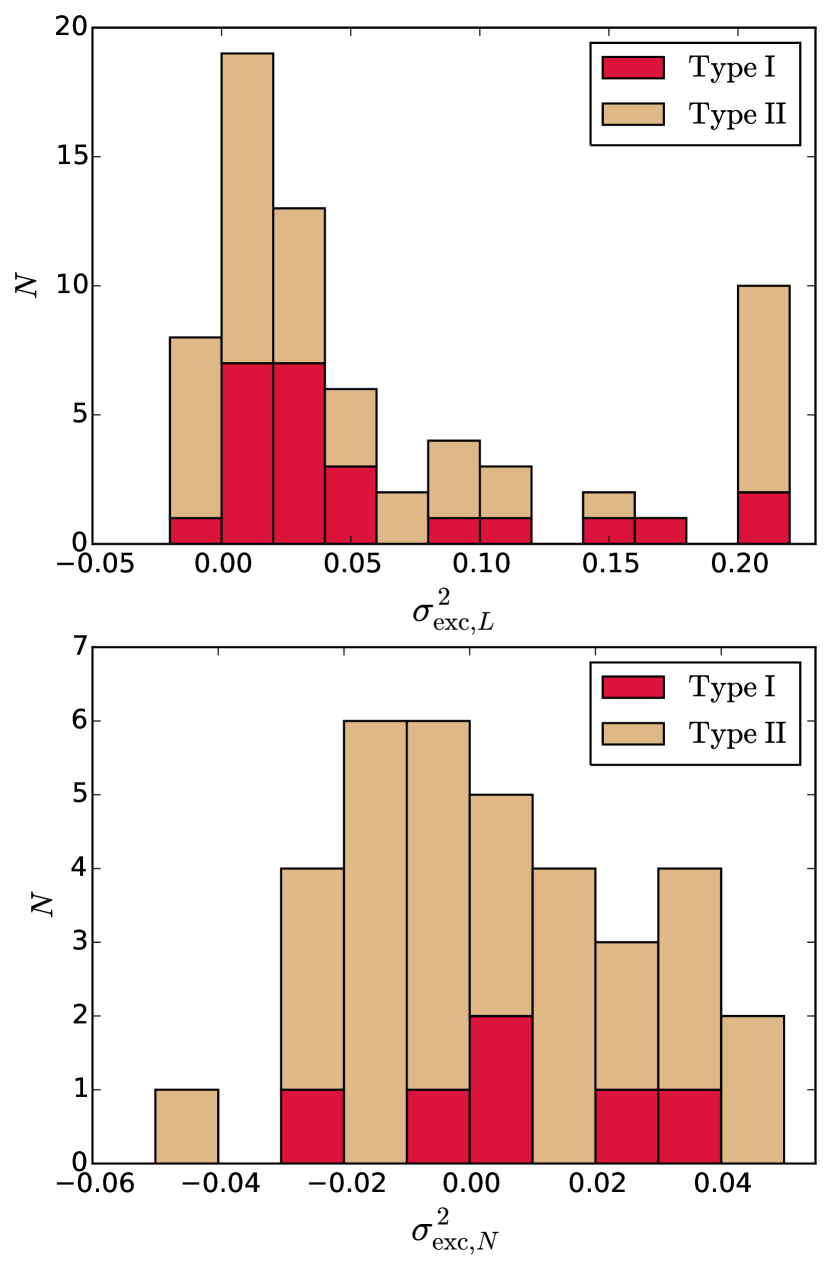
Type I AGNs have a higher $L_{\rm{X}}$ variable source fraction than their type II counterparts (83% vs. 68%), likely due to their higher numbers of counts (Figure 2). Also, type I AGNs have a higher fraction of $N_{\rm{H}}$ variable sources (21% vs. 14%). Figure 10 displays histograms of the ${\sigma^{2}_{\mathrm{exc},L}}$ and ${\sigma^{2}_{\mathrm{exc},N}}$ distributions for different optical spectral types. There are very few type I AGNs in the ${\sigma^{2}_{\mathrm{exc},N}}$ histogram, because most type I AGNs are X-ray unobscured. For the ${\sigma^{2}_{\mathrm{exc},L}}$ distributions, a KS test shows no apparent differences between type I and type II AGNs. Since optical spectral type is often related to the rest-frame optical color (e.g., $u-g$; see Section 2.2), we also check the ${\sigma^{2}_{\mathrm{exc},L}}$ dependence on rest-frame $u-g$ color but do not find a significant relation. The similarity of long-term (years) X-ray variability between type I and type II AGNs has also been found by previous studies of both distant AGNs (e.g., Lanzuisi et al., 2014) and local Compton-thin Seyfert galaxies (e.g., Turner et al., 1997; Hernández-García et al., 2015), though Seyfert IIs tend to be less variable than Seyfert Is on short time scales (minutes to hours) (e.g., Turner et al., 1997; Awaki et al., 2006).

Figure 10.— Upper panel: the ${\sigma^{2}_{\mathrm{exc},L}}$ histogram. The red and brown colors indicate type I and type II AGNs, respectively. A KS test shows the dependence of ${\sigma^{2}_{\mathrm{exc},L}}$ on optical type is not significant. The rightmost column indicates all sources with ${\sigma^{2}_{\mathrm{exc},L}}$ $>0.2$. Lower panel: ${\sigma^{2}_{\mathrm{exc},N}}$ histogram. Only the 35 sources with ${\sigma^{2}_{\mathrm{exc},N}}$ calculated are shown here (Section 3.2.7). The rightmost column indicates all sources with ${\sigma^{2}_{\mathrm{exc},N}}$ $>0.04$.

3.2.8 Variability Dependence on Time Scale

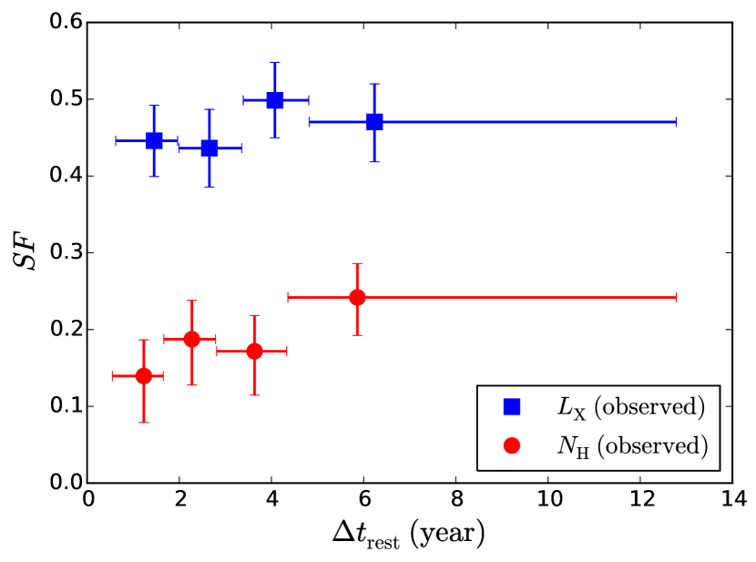
Considering that our light curves are sparsely sampled (with four epochs), we cannot investigate the variability dependence on time scale for each source individually. Instead, we consider our entire sample as an ensemble and investigate its $L_{\rm{X}}$ ($N_{\rm{H}}$) variability on different time scales. We calculate the “structure function” ($SF$, i.e., ensemble-averaged fractional variability amplitude between two observations) as a function of rest-frame time interval ($\Delta t_{\rm rest}$).

First, for each epoch pair of a source (6 pairs in total for each source) we obtain a variability factor

$$f_{v}=\frac{\Delta x}{\overline{x}}=\frac{x_{2}-x_{1}}{(x_{2}+x_{1})/2};$$ (15)

and its uncertainty from error propagation

$$\delta f_{v}=\frac{x_{1}x_{2}}{\overline{x}^{2}}\times\sqrt{\left(\frac{\delta x_{1}}{x_{1}}\right)^{2}+\left(\frac{\delta x_{2}}{x_{2}}\right)^{2}},$$ (16)

where $x_{1}$ and $x_{2}$ are the best-fit $norm_{i}$ ($N_{\rm{H}}$_,i) of two different epochs; $\delta x_{1}$ and $\delta x_{2}$ are their 1$\sigma$ errors. Each $f_{v}$ is associated with a $\Delta t_{\rm rest}$ between two epochs. We then bin $f_{v}$ with similar $\Delta t_{\rm rest}$ and calculate the $SF$ (e.g., Vanden Berk et al., 2004) as

$$SF=\sqrt{\frac{\pi}{2}\langle|f_{v}|\rangle^{2}-\langle(\delta f_{v})^{2}\rangle},$$ (17)

where the angle brackets denote average values in the $\Delta t_{\rm rest}$ bin. We estimate the uncertainties of the $SF$ from bootstrapping, and the results are displayed in Figure 11.

Our 19 quasars generally have weaker variability (Section 3.2.6) and shorter $\Delta t_{\rm rest}$ (due to cosmological time dilation; see Figure  8). Hence, they might cause the $L_{\rm{X}}$ $SF$ to be lower at shorter $\Delta t_{\rm rest}$. To avoid this bias, we do not include them when calculating the $L_{\rm{X}}$ $SF$. The resulting $L_{\rm{X}}$ $SF$ is relatively flat as a function of time scale, with perhaps a suggestion of rising toward longer time scales.

The fractional variability amplitude of $N_{\rm{H}}$ is generally smaller than that of $L_{\rm{X}}$, and appears to increase as $\Delta t_{\rm rest}$ increases. In the $N_{\rm{H}}$ $SF$ calculations, we only include the 35 sources with all four epochs having $\delta N_{\mathrm{H},i}/N_{\mathrm{H},i}<0.4$ (Appendix A).

Figure 11.— Structure functions ($SF$s) as a function of rest-frame time interval, $\Delta t_{\rm rest}$. The blue square points and the red circle points indicate the observed $SF$s for $L_{\rm{X}}$ and $N_{\rm{H}}$, respectively. The $SF$ for $L_{\rm{X}}$ is calculated based on non-quasar ($L_{\rm{X}}$ $<10^{44}$ erg s^-1) sources only to avoid a bias (Section 3.2.8). The error bars of the $SF$s indicate 1$\sigma$ uncertainties calculated from bootstrapping; the error bars of $\Delta t_{\rm rest}$ indicate the bin width.

4. Summary, Discussion, and Future Prospects

In this paper, we have performed long-term (up to $\approx 15$ yr, observed-frame) X-ray variability analyses for the 68 X-ray brightest radio-quiet AGNs in the uniquely deep CDF-S; most of these objects are at redshifts of 0.6–3.1, providing access to penetrating rest-frame X-rays up to $\approx 10-30$ keV. AGNs like those studied here produce a significant fraction of cosmic accretion power; in this sense, they are the typical AGNs of the Universe. We have performed both photometric and spectral variability analyses, and studied the dependence of variability on source properties and time scale. We summarize our main results in Section 4.1. In Section 4.2, we interpret the $L_{\rm{X}}$ variability in the context of AGN PSD. We present practical future extensions to this work in Section 4.3.

4.1. Summary of Main Results

The main results are the following:

1. Photometric analyses (Section 3.1) show that at above a 95% confidence level, 90% (61/68) and 16% (11/68) of our sources are variable in photon flux ($PF$) and hardness ratio ($HR$), respectively. Our results confirm the prevalence of X-ray $PF$ variability for typical AGNs in the distant universe (e.g., Paolillo et al., 2004; Lanzuisi et al., 2014). A large fraction of sources ($\sim 50\%$) is also found to be $PF$-variable within single epochs. However, $HR$ variability is generally insignificant within single epochs ($\mathrel{\hbox to0.0pt{\lower 4.0pt\hbox{\hskip 1.0pt$\sim$}\hss}\raise 1.0pt\hbox{$<$}}1$ yr, observed-frame).

2. Spectral analyses (using a $wabs\times zwabs\times pegpwrlw$ model; see Section 3.2) demonstrate that the $L_{\rm{X}}$- and $N_{\rm{H}}$-variable source fractions are 74% (50/68) and 16% (11/68), respectively. Among the X-ray obscured quasars, the $L_{\rm{X}}$-variable source fraction is also high ($\approx 60\%$); this includes the BAL quasar (J033209.4–274806). Large-amplitude flux variability is rare; most sources (84%) have flux changes within a factor of 2 over 15 yr (observed-frame, see Section 3.2.2). We do not find a significant anticorrelation between $L_{\rm{X}}$ and $N_{\rm{H}}$ variability, as might be expected for a photoionized absorber (see Section 3.2.4).

3. We have quantified the fractional variability scale by calculating the normalized excess variance (${\sigma^{2}_{\rm exc}}$) for each source (see Section 3.2.5). Quasars with $L_{\rm{X}}$ $>10^{44}$ erg s^-1 generally have smaller variability amplitudes than less-luminous AGNs. We have not found any significant dependence of $L_{\rm{X}}$ variability amplitudes on optical spectral type, consistent with the results of Lanzuisi et al. (2014). Therefore, we appear to be observing the X-ray emission of most type II AGNs directly from the central engine; this can occur if X-rays are able to penetrate the obscuring material.

4. We have calculated $SF$s to illustrate the variability dependence on rest-frame time scale (Section 3.2.8). The $L_{\rm{X}}$ $SF$ is relatively flat; the $N_{\rm{H}}$ $SF$ appears to rise toward longer time scales.

5. A Compton-thick AGN candidate (Comastri et al., 2011) in our sample (J033218.3–275055) shows notable X-ray variability. Motivated by Comastri et al. (2011), we used a reflection-dominated $wabs\times zwabs\times pexmon$ model to perform spectral analyses. The results indicate that both the reflection flux and the $N_{\rm{H}}$ are variable (see Appendix B). The variability time scale ($\approx$ a year) indicates the size of the reflecting material is $\mathrel{\hbox to0.0pt{\lower 4.0pt\hbox{\hskip 1.0pt$\sim$}\hss}\raise 1.0pt\hbox{$<$}}0.3$ pc. Nevertheless, it is also possible that the observed X-ray flux is a combination of both transmitted and reflected radiation, and the observed high-energy flux variability is mainly caused by the variable transmitted component.

6. We have identified a source in our sample (J033229.9–274530) that transitions from X-ray unobscured to obscured states over a $\approx 3$ yr rest-frame time scale (see Appendix C). The source is a type I object at $z=1.21$ with $L_{\rm{X}}$$\approx 7\times 10^{43}\ \rm erg\ s^{-1}$. Its $L_{\rm{X}}$ is higher when it is less X-ray obscured. The angular size of an X-ray eclipsing cloud is estimated to be several degrees (viewed from the central SMBH). However, there is no corresponding optical spectral-type transition, suggesting that the X-ray eclipsing material is too small to block most of the broad-line emission.

4.2. Interpretation from Power Spectral Density

The observed low $L_{\rm{X}}$ variability amplitudes of quasars can be plausibly explained by the AGN PSD, which describes variability power as a function of frequency. An AGN PSD can often be well modeled as a broken power law (e.g., Uttley et al., 2002)

$$\mathrm{PSD}(\nu)=\begin{cases}\mathrm{PSD_{amp}}\nu^{-1},\ \mathrm{if}\ \nu<\nu_{\rm bf};\\ \mathrm{PSD_{amp}}\nu_{\rm bf}\nu^{-2},\ \mathrm{if}\ \nu\geq\nu_{\rm bf}.\end{cases}$$ (18)

The normalization $\mathrm{PSD_{amp}}$ is roughly constant ($0.017\pm 0.006$), according to studies of Seyfert galaxies (Papadakis, 2004). The low-frequency power law extends at least to several-year time scales in local Seyfert galaxies (e.g., Zhang, 2011). $\nu_{\rm bf}$ is related to both SMBH mass ($M_{\mathrm{BH}}$) and bolometric luminosity ($L_{\rm bol}$) as (McHardy et al., 2006)

$$\begin{split}\nu_{\rm bf}&\sim 50\left(\frac{M_{\rm BH}}{10^{8}M_{\sun}}\right)^{-2}\left(\frac{L_{\rm bol}}{10^{45}\ \mathrm{erg\ s^{-1}}}\right)\ \mathrm{yr^{-1}}\\ &\sim 10\left(\frac{L_{\rm X}}{10^{44}\ \mathrm{erg\ s^{-1}}}\right)^{-1}\left(\frac{k_{\rm bol}}{50}\right)^{-1}\left(\frac{\lambda_{\rm Edd}}{0.1}\right)^{2}\mathrm{yr^{-1}}\end{split}$$ (19)

where $\lambda_{\mathrm{Edd}}$ and $k_{\mathrm{bol}}$ are the Eddington ratio and bolometric correction factor for $L_{\rm{X}}$ (2–10 keV), respectively. Given a PSD of a source, the ${\sigma^{2}_{\mathrm{exc},L}}$ can be estimated as (e.g., Papadakis, 2004; Papadakis et al., 2008)

$$\begin{split}\sigma_{\mathrm{exc},L}^{2}&=\int^{\nu_{\rm hf}}_{\nu_{\rm lf}}\mathrm{PSD}(\nu)\mathrm{d}\nu\\ &=\mathrm{PSD_{amp}}\ln\left(\frac{\nu_{\mathrm{h}f}}{\nu_{\mathrm{l}f}}\right),\ \mathrm{if}\ \nu_{\rm hf}<\nu_{\rm bf}.\end{split}$$ (20)

The integral bounds for our study are

$$\begin{split}\nu_{\rm lf}&\sim\frac{1+z}{t_{\rm span}}\ \mathrm{and}\\ \nu_{\rm hf}&\sim\frac{1+z}{t_{\rm bin}},\\ \end{split}$$ (21)

respectively, where $t_{\rm span}=14.3$ yr is the observed-frame total observation span and $t_{\rm bin}=0.46$ yr is the observed-frame median bin width of the four epochs. For an AGN with $L_{\rm{X}}$$=10^{44}$ erg s^-1 and $\lambda_{\mathrm{Edd}}\sim 0.1$, the typical bolometric correction factor is $k_{\mathrm{bol}}\sim 50$ (e.g., Hopkins et al., 2007), and the typical redshift is $\approx 2$ (see Figure 8). Thus, Equations 19 and 21 yield $\nu_{\rm bf}\sim\nu_{\rm hf}\sim 10$ yr^-1. For AGNs with higher luminosity (i.e., quasars), both $k_{\mathrm{bol}}$ and $z$ tend to be larger. $\nu_{\rm hf}$ and $\nu_{\rm bf}$ will increase and decrease, respectively (assuming the same $\lambda_{\mathrm{Edd}}$); e.g., for a typical quasar at $z\sim 3$ with $L_{\rm{X}}$$\sim 3\times 10^{44}$ erg s^-1 (see Figure 8), $\nu_{\rm bf}$ will increase by a factor of $\sim 1.3$ due to $z$, and $\nu_{\rm hf}$ will decrease at least 3 times due to $L_{\rm{X}}$ and $k_{\mathrm{bol}}$. Therefore, $\nu_{\rm hf}$ is likely to be higher than $\nu_{\rm bf}$ for quasars (Equations 19 and 21), i.e., the integral range in Equation 20 covers the power law with slope $-2$ that drops strongly toward high frequency. The resulting $\sigma_{\mathrm{exc},L}$ for quasars should thus be smaller than for other AGNs, consistent with observations (Section 3.2.6). For a non-quasar AGN, we might be sampling only the low-frequency part of its PSD with slope $-1$ (i.e., $\nu_{\rm hf}<\nu_{\rm bf}$); Equations 20 and 21 result in an approximately constant ${\sigma^{2}_{\mathrm{exc},L}}$ value of $0.059\pm 0.021$, regardless of source properties. This ${\sigma^{2}_{\mathrm{exc},L}}$ value is generally lower than the observed values for our non-quasar AGNs (see Figure 9), casting doubt on the universality of the constant-amplitude PSD model (e.g., Ponti et al. 2012; M. Paolillo et al., in preparation).

4.3. Future Work

Considering reasonably in-depth studies of the long-term X-ray variability of typical distant AGNs, it will be difficult to surpass greatly the present work for a considerable period of time; this is primarily due to the unmatched CDF-S exposure obtained over the extended period of $\approx 15$ yr. Additional X-ray variability studies should be done for the large population of X-ray fainter CDF-S AGNs (see Figure 8; e.g., X. C. Zheng et al., in preparation), although it will be more difficult to characterize these systems individually in depth. If Chandra continues to operate for another $\approx 10$ yr, as appears plausible (e.g., Wilkes, 2015), obtaining additional CDF-S exposure in several years could lengthen our time baseline to up to $\approx 25$ yr in total. The Advanced Telescope for High Energy Astrophysics (Athena; e.g., Barcons et al. 2015), planned for launch in $\approx 13$ yr, has the best current prospects for substantially advancing long-term X-ray variability studies of typical AGNs in the distant universe. Owing to its greatly improved photon collecting area, it will obtain much better photon statistics for its deep-field AGNs. With suitable observation scheduling, it could efficiently perform a study similar to that in this work but for many more objects and with tens of epochs of observations spanning a wide range of timescales. The prime deep-survey field for Athena is arguably the CDF-S, and Athena variability studies could build upon the long-term baseline of Chandra CDF-S observations utilized in this work.

Appendix A Error Estimation of Model Parameters

As described in Section 3.2.1, we fit spectra of the four epochs simultaneously with a $wabs\times zwabs\times pegpwrlw$ model. The photon index, $\Gamma$, is linked across the four epochs, assuming no $\Gamma$ variability (see Section 3.2.1 for the justification of this assumption). In this Appendix, we first explain our choice of $pegpwrlw$ over $powerlaw$, and then describe our method to estimate the errors of $N_{\rm{H}}$_,i.

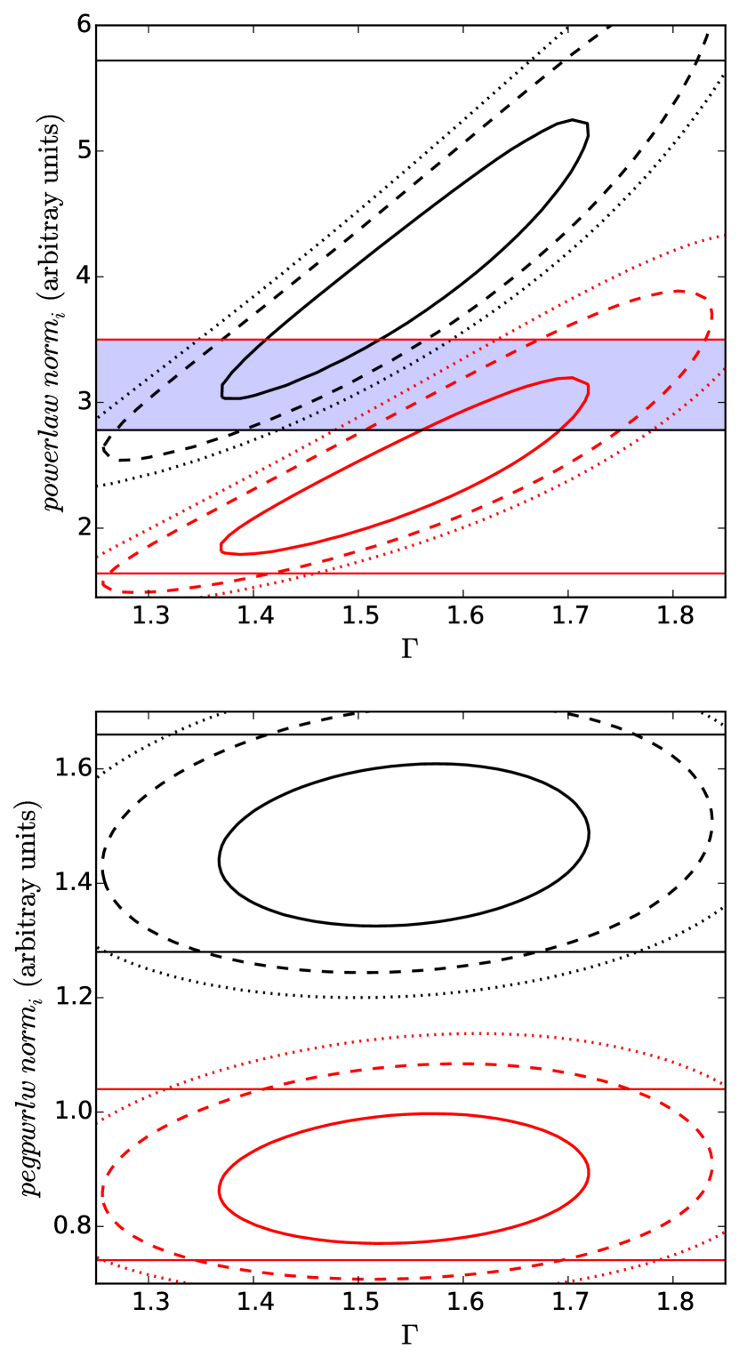
As an illustrative example, we show the $norm_{i}$-$\Gamma$ confidence contours of the first two epochs of J033217.1–275220 resulting from fitting with a model of $wabs\times zwabs\times powerlaw$ (see the upper panel of Figure 12). The contours, as expected, show positive correlations between $norm_{i}$ and $\Gamma$. Since no overlapping region exists between the two 99% confidence contours, the probability of the two epochs having both the same $norm_{i}$ and $\Gamma$ is very low [$<(1-99\%)^{2}=0.01\%$]. Therefore, the $norm_{i}$ variability must be very significant ($>1-0.01\%=99.99\%$) under our assumption of constant $\Gamma$. However, if we evaluate the $norm_{i}$ variability by checking the 1-dimensional (1D) errors ($2\sigma$) of $norm_{i}$ (the projected range on the $y$-axis), the variability seems to be less significant due to the existence of an overlapping interval (blue shaded region). More quantitatively, if we perform a $\chi^{2}$ test of the $norm_{i}$ variability using the best-fit values and 1D errors, the resulting significance of variability is only 93%. This apparent discrepancy occurs because when calculating the 1D errors of $norm_{i}$ by projecting the 2D contours, the positive $norm_{i}-\Gamma$ correlations and our underlying assumption of constant $\Gamma$ are “forgotten”. This is evident since the blue-shaded region only covers the two dashed contours at very different $\Gamma$, i.e., the same $norm_{i}$ can be achieved only when the assumption of constant $\Gamma$ is violated. Reading Figure 12, $\Gamma$ would need to change by $\Delta\Gamma\approx 0.2-0.3$, and this is larger than any physically expected $\Gamma$ change (see Section 3.2.1). Therefore, the errors of $norm_{i}$ are overestimated under this assumption of constant $\Gamma$. This problem is prevalent when using $powerlaw$, since positive correlations exist for almost all sources. However, the positive correlations can be mostly eliminated by replacing $powerlaw$ with $pegpwrlw$ (see the lower panel of Figure 12). $pegpwrlw$ differs from $powerlaw$ by having its normalization based on intrinsic flux in a given finite band rather than the flux density at observed-frame 1 keV. We find that setting the normalization band as $E_{peg}-7$ keV produces nearly horizontal $norm_{i}$-$\Gamma$ contours for all sources, where $E_{peg}$ is the minimum between 0.5 keV and the observed-frame $e$-folding energy ($E_{\rm fold}$) caused by intrinsic photoelectric absorption. Technically, we obtain the photoelectric cross section $\sigma_{\rm photo}$ as a function of energy (Morrison & McCammon, 1983), and solve the equation $\langle N_{\rm H}\rangle\times\sigma_{\rm photo}[E_{\rm fold}\times(1+z)]=1$ to obtain $E_{\rm fold}$, where the factor $1+z$ is to convert observed-frame to rest-frame energy.

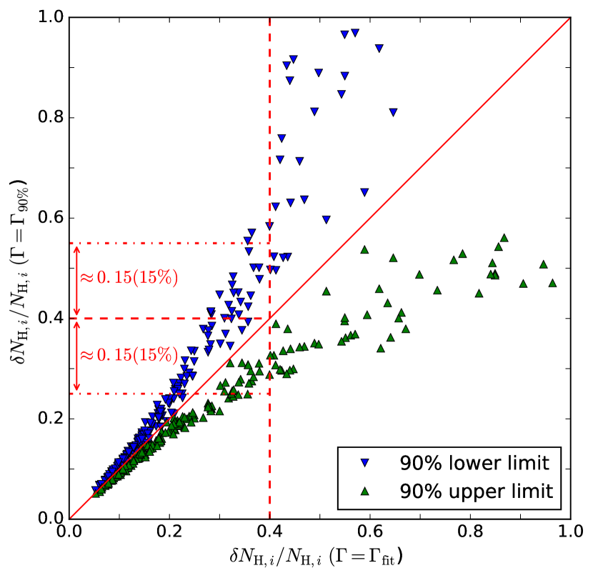
Similar positive correlations are also, as expected, prevalent in the $N_{\rm{H}}$_,i-$\Gamma$ contours. However, we are not aware of any model choices that can eliminate these correlations (as for the choice of $pegpwrlw$ in the $norm_{i}$ case). Alternatively, if intrinsic $\Gamma$ ($\Gamma_{\rm intr}$) were given, one could fix $\Gamma=\Gamma_{\rm intr}$ and estimate the the errors of $N_{\rm{H}}$_,i. But in reality, $\Gamma_{\rm intr}$ is not perfectly known. We thus adopt an approximation, i.e., fixing $\Gamma=\Gamma_{\rm fit}$. The idea is to approximate $\Gamma_{\rm intr}$ as $\Gamma_{\rm fit}$. Admittedly, compared to fixing $\Gamma=\Gamma_{\rm intr}$, this approximation might overestimate or underestimate the errors of $N_{\rm{H}}$_,i. To evaluate this possible issue, we fix $\Gamma$ at the 90% confidence lower and upper limits of $\Gamma_{\rm fit}$, respectively, and then estimate the errors. The lower and upper limits approximate the boundaries of possible $\Gamma_{\rm intr}$ values. If fixing $\Gamma$ at these boundaries results in similar errors as fixing $\Gamma$ at $\Gamma_{\rm fit}$, we conclude that our approximation (i.e., fixing $\Gamma=\Gamma_{\rm fit}$) gives accurate errors of $N_{\rm{H}}$_,i for a given source. Figure 13 shows the results. The dependence of estimated fractional error $\delta N_{\mathrm{H},i}/N_{\mathrm{H},i}$ on $\Gamma$ is stronger when the error is larger. In Figure 13, at $\delta N_{\mathrm{H},i}/N_{\mathrm{H},i}=0.4$ (the vertical dashed line), fixing $\Gamma$ at its 90%-confidence lower and upper limits of $\Gamma_{\rm fit}$ results in $\delta N_{\mathrm{H},i}/N_{\mathrm{H},i}\mathrel{\hbox to0.0pt{\lower 4.0pt\hbox{\hskip 1.0pt$\sim$}\hss}\raise 1.0pt\hbox{$<$}}0.55$ and $\mathrel{\hbox to0.0pt{\lower 4.0pt\hbox{\hskip 1.0pt$\sim$}\hss}\raise 1.0pt\hbox{$>$}}0.25$, respectively (the dash-dotted lines). Since $\Gamma_{\rm intr}$ is very likely within the range of the 90% limits of $\Gamma_{\rm fit}$, fixing $\Gamma=\Gamma_{\rm intr}$ (if it were perfectly known) should give $\delta N_{\mathrm{H},i}/N_{\mathrm{H},i}$ within the range of $\approx 0.25-0.55$. Therefore, fixing $\Gamma=\Gamma_{\rm intr}$ would lead to $\delta N_{\mathrm{H},i}/N_{\mathrm{H},i}$ deviating from that obtained by our approximation (fixing $\Gamma=\Gamma_{\rm fit}$) by $\mathrel{\hbox to0.0pt{\lower 4.0pt\hbox{\hskip 1.0pt$\sim$}\hss}\raise 1.0pt\hbox{$<$}}15\%$ (i.e., $15\%=0.15=0.55-0.4=0.4-0.25$). For epochs with $\delta N_{\mathrm{H},i}/N_{\mathrm{H},i}<0.4$, this value should be even lower. In the analyses where errors on $N_{\rm{H}}$_,i are being used (Sections 3.2.6 and 3.2.8), we only include the 35 sources with all four epochs having $\delta N_{\mathrm{H},i}/N_{\mathrm{H},i}<0.4$. This criterion guarantees that the $N_{\rm{H}}$_,i fractional errors estimated by fixing $\Gamma=\Gamma_{\rm fit}$ differ from those estimated by fixing $\Gamma=\Gamma_{\rm intr}$ by $\mathrel{\hbox to0.0pt{\lower 4.0pt\hbox{\hskip 1.0pt$\sim$}\hss}\raise 1.0pt\hbox{$<$}}15\%$. Though not ideal, this criterion is a practical solution for our $N_{\rm{H}}$ variability analyses, balancing between the accuracy of error estimation and the sample size.

Figure 12.— $norm_{i}-\Gamma$ confidence contours of the first two epochs of J033217.1–275220 resulting from modelling with $wabs\times zwabs\times powerlaw$ (upper panel) and $wabs\times zwabs\times pegpwrlw$ (lower panel). Black and red colors indicate epochs 1 and 2, respectively. The solid, dashed, and dotted curves indicate 1$\sigma$ (68%), 2$\sigma$ (95%), and 99% confidence contours, respectively. The horizontal solid lines indicate the 2$\sigma$ uncertainty ranges of $norm_{i}$. In the upper panel, the 99% confidence contours do not overlap, indicating highly significant variability of $norm_{i}$ (i.e., $>99.99\%$ confidence level; see Appendix A). However, the two projected $norm_{i}$ uncertainty ranges have an overlapping interval (blue shaded region), and a $\chi^{2}$ test shows that the significance level of $norm_{i}$ variability is only 93%. Thus, the errors of $norm_{i}$ are overestimated under the assumption of constant $\Gamma$. In the lower panel, this issue does not occur.

Figure 13.— Fractional errors $\delta N_{\mathrm{H},i}/N_{\mathrm{H},i}$ obtained by fixing $\Gamma$ at the 90% confidence limits of $\Gamma_{\rm fit}$ vs. those obtained by fixing $\Gamma$ at the best-fit value. The green upward-pointing and blue downward-pointing triangles indicate the fractional errors obtained by fixing $\Gamma$ at the upper and lower limits of $\Gamma_{\rm fit}$, respectively. The red solid line indicates the ideal situation, i.e., the estimated fractional errors are not affected by fixing $\Gamma$ at different values. The vertical red dashed line indicates our threshold, i.e., only sources with all four epochs having $\delta N_{\mathrm{H},i}/N_{\mathrm{H},i}<0.4$ are included in the analyses where errors on $N_{\rm{H}}$_,i are being used. Its intersection points with the approximate outer envelopes of the blue and green triangles are indicated by the horizontal red dash-dotted lines, and their deviations from $\delta N_{\mathrm{H},i}/N_{\mathrm{H},i}=0.4$ (the horizontal red dashed line) are $\approx 0.15$ (15%, as marked). Our sample consists 68 sources with each of them having 4 epochs. Thus, there are 272 ($68\times 4$) pairs of triangles plotted (though some are located out of the plotted ranges and are not shown). Note that for each source, the $\delta N_{\mathrm{H},i}/N_{\mathrm{H},i}$ ($x$-axis) are different for different epochs.

Appendix B A Highly Variable Compton-Thick Candidate

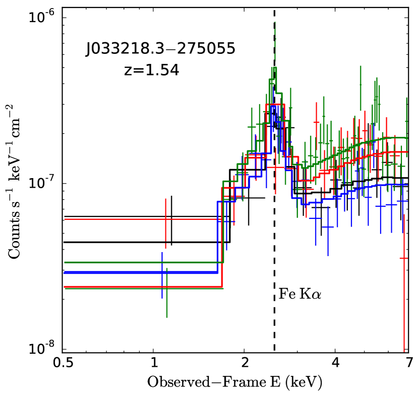
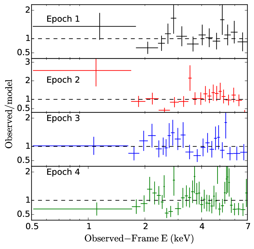
J033218.3–275055 is a bright Compton-thick candidate AGN at $z=1.54$ reported in the literature (Tozzi et al., 2006; Comastri et al., 2011). It is classified as an optical type II object. It shows a strong Fe K$\alpha$ emission line with a rest-frame equivalent width (REW) of $\approx 1.2$ keV (Comastri et al., 2011). Our spectral fitting confirms its highly obscured nature ($N_{\mathrm{H}}=3\times 10^{23}\ \mathrm{cm^{-2}}$). Both its $L_{\rm{X}}$ and $N_{\rm{H}}$ values are variable ($\Delta\mathrm{AIC}_{L}=38$ and $\Delta\mathrm{AIC}_{N}=5.1$). However, its high $goodness$ (44%) and low $\Gamma$ (1.2, i.e., our allowed lower limit, see Section 3.2.1) indicate the model $wabs\times zwabs\times pegpwrlw$ is likely inappropriate (see Figure 6). Thus, motivated by Comastri et al. (2011), we use the model $wabs\times zwabs\times pexmon$ (for $pexmon$, see Magdziarz & Zdziarski, 1995; Nandra et al., 2007) to fit the data. We set the $pexmon$ model to be fully reflection dominated and fix the inclination angle at 60°. We link the $\Gamma$ ($pexmon$) of all four epochs, and set $norm_{i}$ ($pexmon$) and $N_{\rm{H}}$_,i ($zwabs$) free (not linked). The fitted spectra of the reflection-dominated model are shown in Figure 14, and the detailed fitting results are presented in Table 4.

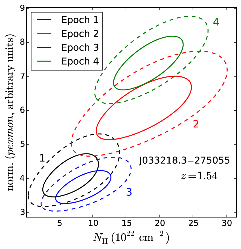
Despite having the same number of degrees of freedom as the previous model ($wabs\times zwabs\times pegpwrlw$), the new fitting results in a $goodness=8\%$ and best-fit $\Gamma=1.80$, values that are more common among the $goodness$ and $\Gamma$ distributions for our overall sample (see Figure 6). Also, the new model has AIC much smaller than the previous model ($\Delta\rm AIC=54$), indicating a significant improvement in the fit quality. Thus, we consider this reflection-dominated model to be more physically plausible than the simple transmission-dominated model. Following Section 2.4.1 of Nandra et al. (2007), this $\Gamma$ value (i.e., 1.80) results in an REW of Fe K$\alpha$ ($pexmon$) of $\approx 1.4$ keV, consistent with Comastri et al. (2011). Similar to the approach in Section 3.2.3, we test the significance of reflection-flux and $N_{\rm{H}}$ variability by linking $norm_{i}$ ($pexmon$) and $N_{\rm{H}}$_,i, respectively. The increased AIC values (i.e., 39 and 4.2) are both greater than 4, indicating both the reflection flux and $N_{\rm{H}}$ are variable (Section 3.2.3). The confidence contours are shown in Figure 15. Both the absorption and continuum are weak in epoch 1; they rise in epoch 2 and then drop in epoch 3; in epoch 4, they rise again. The amplitude of flux variability is large; e.g., the flux in epoch 4 is almost twice that in epochs 1 and 3. The variability time scale ($\approx$ a year) constrains the size of the reflecting material to be $\mathrel{\hbox to0.0pt{\lower 4.0pt\hbox{\hskip 1.0pt$\sim$}\hss}\raise 1.0pt\hbox{$<$}}0.3$ pc.

However, there is a possible alternative explanation for the observed high-energy flux variability of this source, though our reflection-dominated model explains the data satisfactorily. The observed X-ray emission might be a combination of both transmitted and reflected radiation. In this scenario, the transmission component is variable and results in the observed high-energy flux variability, while the reflection component is stable. To test this scenario, we use a $wabs\times zwabs\times(pegpwrlw+pexmon)$ model. We assume that the $pegpwrlw$ and $pexmon$ components share the same non-variable $\Gamma$, and the normalization of $pexmon$ is the same across epochs. The $N_{\rm{H}}$ ($zwabs$) and the normalization of $pegpwrlw$ are allowed to vary across epochs. Other parameters of the $pexmon$ component are the same as for the reflection-dominated model. This composite model yields $\Gamma=1.5$ and $goodness=5\%$, similar to that of the reflection-dominated model. The resulting transmitted flux almost completely shuts down at epoch 1 and epoch 3 (more than an order of magnitude smaller than at epoch 2 and epoch 4). Such strong variability is not likely to be realistic, considering the general variability amplitudes of our sources (see Section 3.2.2). Nevertheless, more complex transmission-reflection hybrid models might produce more physically plausible results, though they cannot be constrained well owing to the available number of counts.

Figure 14.— Upper panel: unfolded (i.e., intrinsic) spectra for the Compton-thick candidate J033218.3–275055 using fitting model $wabs\times zwabs\times pexmon$. The solid lines indicate best-fit model photon-flux density. Different colors indicate different epochs. The vertical dashed line indicates the energy of Fe K$\alpha$ line (i.e., rest-frame 6.4 keV). Data are binned for display purposes only. Note that the flux in the high-energy band (less affected by absorption) varies significantly. Lower panel: ratio of observed and model photon flux.

Table 4Spectral Fitting^a Results of the Compton-Thick Candidate (J033218.3–275055)

Epoch	$\Gamma$	$N_{\rm{H}}$	fluxb
		($10^{22}\rm\ cm^{-2}$)	($10^{-15}\rm\ erg\ cm^{-2}\ s^{-1}$)
1	1.80	$5.61^{+2.88}_{-2.38}$	$4.16^{+0.34}_{-0.40}$
2	–	$17.00^{+4.80}_{-4.40}$	$5.47^{+0.44}_{-0.46}$
3	–	$7.81^{+2.89}_{-2.52}$	$3.71^{+0.26}_{-0.26}$
4	–	$17.80^{+3.60}_{-3.30}$	$6.64^{+0.33}_{-0.35}$

Note. —
a. The spectral fitting model is $wabs\times zwabs\times pexmon$ (see Section B).
b. Full-band (0.5–7 keV) model flux, not corrected for Galactic or intrinsic absorption.

Figure 15.— Confidence contours of the normalizations of $pexmon$ and $N_{\rm{H}}$ for source J033218.3–275055, the Compton-thick candidate. The solid and dashed curves indicate $1\sigma$ and $2\sigma$ confidence contours, respectively. Different colors indicate different epochs, and the epoch indexes are also labeled beside the corresponding contours.

Appendix C Three Significantly Variable Sources

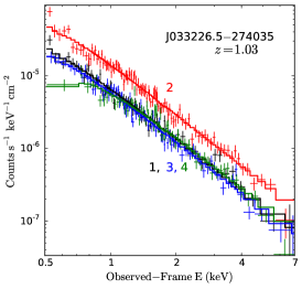
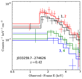
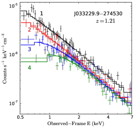
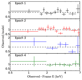
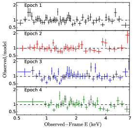
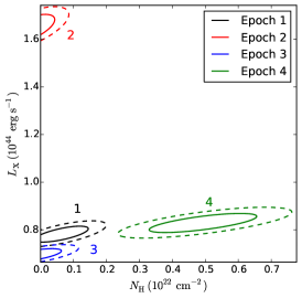
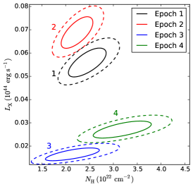
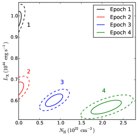
As illustrative examples, we investigate three significantly variable sources. The first source, J033226.5–274035 ($z=1.03$), is our brightest source; it also has the most significant $L_{\rm{X}}$ variability. The second source, J033259.7–274626 ($z=0.42$), is also $L_{\rm{X}}$-variable, but has counts typical in our sample; this source is shown as a representative sample member. The third source, J033229.9–274530 ($z=1.21$), has the most significant $N_{\rm{H}}$ variability; it transitions from an X-ray unobscured to obscured state. Their fitted spectra and $L_{\rm{X}}$–$N_{\rm{H}}$ confidence contours are shown in Figure 16.

J033226.5–274035 has the largest number of total net counts ($\approx$11000). It has $\Delta\mathrm{AIC}_{L}=1059$ and $\Delta\mathrm{AIC}_{N}=15$, indicating both $L_{\rm{X}}$ and $N_{\rm{H}}$ variability. The $\Delta\mathrm{AIC}_{L}$ is the largest among those of our sources. Its $L_{\rm{X}}$ in the second epoch is about two times the $L_{\rm{X}}$ in the other epochs. Its $N_{\rm{H}}$ is generally low: $N_{\rm{H}}$ only has upper limits in the first three epochs and rises to $\approx 4\times 10^{21}\ \mathrm{cm^{-2}}$ in the last epoch. J033226.5–274035 and another bright (net counts $\approx 6500$) and variable source ($\Delta\mathrm{AIC}_{L}=38$, $\Delta\mathrm{AIC}_{N}=5.1$), J033218.3–275055, are also identified as optically variable sources by Falocco et al. (2015) based on their $r$-band variability.

J033259.7–274626 has total net counts of $\approx$1300, similar to the median counts of our sample (1399). It has $\Delta\mathrm{AIC}_{L}=165$, indicating significant $L_{\rm{X}}$ variability. Its $L_{\rm{X}}$ values in the first two epochs are about three times higher than those in the last two epochs. It is X-ray obscured (i.e., $N_{\rm{H}}$$>10^{22}$ cm^-2) with no significant $N_{\rm{H}}$ variability detected ($\Delta\mathrm{AIC}_{N}=-0.9$).

J033229.9–274530 has $\Delta\mathrm{AIC}_{L}=144$ and $\Delta\mathrm{AIC}_{N}=83$ with a total net counts of $\approx 5000$. It is the most significantly $N_{\rm{H}}$ variable source (i.e., has maximum $\Delta\mathrm{AIC}_{N}$). The $N_{\rm{H}}$ values in the first two epochs are low (consistent with zero). The $N_{\rm{H}}$ rises in epoch 3 and reaches $\approx 2\times 10^{22}\rm\ cm^{-2}$ in epoch 4. Its $L_{\rm{X}}$ in epoch 1 is $\approx 2$ times higher than $L_{\rm{X}}$ in the other epochs. The X-ray type transition happens between epochs 2 and 4, and thus corresponds to a rest-frame time scale $t_{\rm tran}\sim 3$ year. If we interpret the transition as an “eclipse” event, this long time scale indicates the eclipsing material is located at a distance larger than that of the BLR from the central engine. This is because BLR-cloud eclipses are likely to happen on much shorter time scales (hours to days; e.g., Maiolino et al. 2010; Wang et al. 2010). Assuming that the eclipsing material is in a single “cloud” within the inner torus region, its distance ($r$) from the central engine is $\sim 0.1$ pc. Applying Kepler’s 3rd law, we can calculate its orbital period

$$\begin{split}t_{\mathrm{orbit}}&=2\pi\frac{r^{\frac{3}{2}}}{(M_{\mathrm{BH}}G)^{\frac{1}{2}}}\\ &\sim 300\left(\frac{M_{\mathrm{BH}}}{10^{8}\ M_{\odot}}\right)^{-\frac{1}{2}}\ \mathrm{yr}.\end{split}$$ (C1)

Then we can estimate the angular size of the cloud, $\theta$ (viewed from the central SMBH), as

$$\begin{split}\theta&\sim\frac{t_{\rm tran}}{t_{\mathrm{orbit}}}\times 360^{\circ}\\ &\sim 4^{\circ}\left(\frac{M_{\mathrm{BH}}}{10^{8}\ M_{\odot}}\right)^{\frac{1}{2}}.\end{split}$$ (C2)

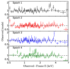
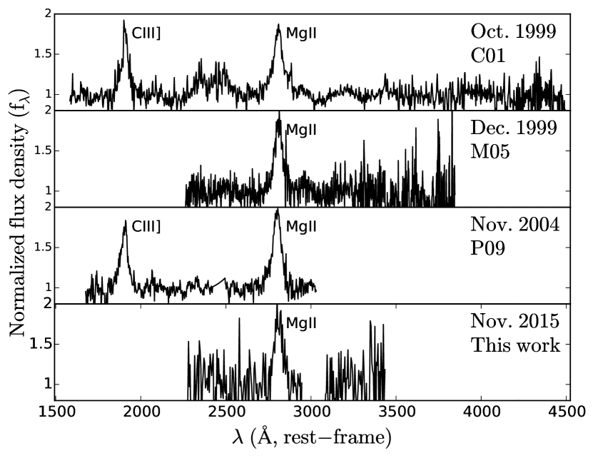
To investigate if the optical spectral type also changes, we have compiled three optical spectra from the literature (Croom et al., 2001; Mignoli et al., 2005; Popesso et al., 2009) and obtained a new spectrum on November 8, 2015. The new observation was performed using the IMACS Short-Camera of the 6.5m Magellan Telescope. The four spectra are presented in Figure 17. In all four spectra, the broad Mg ii $\lambda$2798 line is detected. In the first and third spectra, the C iii] $\lambda$1909 line is also detected. Thus, the optical spectral type of this source remains type I in all four spectra. The lack of optical spectral-type transitions indicates the X-ray eclipsing material is not large enough to block most emission from the BLR. This result is consistent with recent studies of optical spectral-type transition AGNs that suggest significant changes ($\sim 10$ times) in luminosity as the main cause of transitions (e.g., LaMassa et al., 2015; Runnoe et al., 2016).

Figure 16.— Upper panels: unfolded (i.e., intrinsic) spectra for J033226.5–274035, J033259.7–274626, and J033229.9–274530, respectively. The solid lines indicate best-fit model photon flux. Different colors indicate different epochs, and the epoch indexes are also labeled beside the corresponding spectra. Data are binned for display purposes only. Middle panels: the corresponding ratios of observed and model photon-flux density. Lower panels: the corresponding $L_{\rm{X}}$-$N_{\rm{H}}$ confidence contours. J033226.5–274035 has significantly higher luminosity in epoch 2. The luminosity of J033259.7–274626 drops by a large factor ($\approx 3$) since epoch 3. For J033229.9–274530, the spectral shape changes obviously among epochs.

Figure 17.— Normalized optical spectra of J033229.9–274530 at $z=1.21$. The observation dates and the references are listed in the upper-right corner of each panel (C01: Croom et al. 2001; M05: Mignoli et al. 2005; P09: Popesso et al. 2009). The Mg ii $\lambda$2798 broad emission line is present in all four spectra.

References

- Abdo et al. (2010) Abdo, A. A., Ackermann, M., Ajello, M., et al. 2010, ApJ, 722, 520
- Aird et al. (2015) Aird, J., Coil, A. L., Georgakakis, A., et al. 2015, MNRAS, 451, 1892
- Akaike (1974) Akaike, H. 1974, Automatic Control, IEEE Transactions on, 19, 716
- Allevato et al. (2013) Allevato, V., Paolillo, M., Papadakis, I., & Pinto, C. 2013, ApJ, 771, 9
- Almaini et al. (2000) Almaini, O., Lawrence, A., Shanks, T., et al. 2000, MNRAS, 315, 325 (A00)
- Arévalo et al. (2014) Arévalo, P., Bauer, F. E., Puccetti, S., et al. 2014, ApJ, 791, 81
- Arnaud (1996) Arnaud, K. A. 1996, in Astronomical Society of the Pacific Conference Series, Vol. 101, Astronomical Data Analysis Software and Systems V, ed. G. H. Jacoby & J. Barnes, 17
- Awaki et al. (2006) Awaki, H., Murakami, H., Ogawa, Y., & Leighly, K. M. 2006, ApJ, 645, 928
- Barcons et al. (2015) Barcons, X., Nandra, K., Barret, D., et al. 2015, Journal of Physics Conference Series, 610, 012008
- Barger et al. (2003) Barger, A. J., Cowie, L. L., Capak, P., et al. 2003, AJ, 126, 632
- Bauer et al. (2015) Bauer, F. E., Arévalo, P., Walton, D. J., et al. 2015, ApJ, 812, 116
- Begelman et al. (2008) Begelman, M. C., Fabian, A. C., & Rees, M. J. 2008, MNRAS, 384, L19
- Bonzini et al. (2013) Bonzini, M., Padovani, P., Mainieri, V., et al. 2013, MNRAS, 436, 3759
- Brandt et al. (1997) Brandt, W. N., Fabian, A. C., Takahashi, K., et al. 1997, MNRAS, 290, 617
- Brightman et al. (2013) Brightman, M., Silverman, J. D., Mainieri, V., et al. 2013, MNRAS, 433, 2485
- Broos et al. (2010) Broos, P. S., Townsley, L. K., Feigelson, E. D., et al. 2010, ApJ, 714, 1582
- Buchner et al. (2014) Buchner, J., Georgakakis, A., Nandra, K., et al. 2014, A&A, 564, A125
- Burnham & Anderson (2002) Burnham, K. P., & Anderson, D. R. 2002, Model selection and multimodel inference: a practical information-theoretic approach (Springer Science & Business Media)
- Cash (1979) Cash, W. 1979, ApJ, 228, 939
- Chartas et al. (2009) Chartas, G., Saez, C., Brandt, W. N., Giustini, M., & Garmire, G. P. 2009, ApJ, 706, 644
- Civano et al. (2016) Civano, F., Marchesi, S., Comastri, A., et al. 2016, ApJ, 819, 62
- Collinge et al. (2001) Collinge, M. J., Brandt, W. N., Kaspi, S., et al. 2001, ApJ, 557, 2
- Comastri et al. (2011) Comastri, A., Ranalli, P., Iwasawa, K., et al. 2011, A&A, 526, L9
- Connolly et al. (2016) Connolly, S. D., McHardy, I. M., Skipper, C. J., & Emmanoulopoulos, D. 2016, MNRAS, 459, 3963
- Corral et al. (2015) Corral, A., Georgantopoulos, I., Watson, M. G., et al. 2015, A&A, 576, A61
- Croom et al. (2001) Croom, S. M., Warren, S. J., & Glazebrook, K. 2001, MNRAS, 328, 150
- Falocco et al. (2015) Falocco, S., Paolillo, M., Covone, G., et al. 2015, A&A, 579, A115
- Fausnaugh et al. (2015) Fausnaugh, M. M., Denney, K. D., Barth, A. J., et al. 2015, ArXiv e-prints, arXiv:1510.05648
- Filiz Ak et al. (2013) Filiz Ak, N., Brandt, W. N., Hall, P. B., et al. 2013, ApJ, 777, 168
- Gallagher et al. (2002) Gallagher, S. C., Brandt, W. N., Chartas, G., & Garmire, G. P. 2002, ApJ, 567, 37
- Gallagher et al. (2006) Gallagher, S. C., Brandt, W. N., Chartas, G., et al. 2006, ApJ, 644, 709
- Gallagher et al. (2004) Gallagher, S. C., Brandt, W. N., Wills, B. J., et al. 2004, ApJ, 603, 425
- Garmire et al. (2003) Garmire, G. P., Bautz, M. W., Ford, P. G., Nousek, J. A., & Ricker, Jr., G. R. 2003, in Proc. SPIE, Vol. 4851, X-Ray and Gamma-Ray Telescopes and Instruments for Astronomy., ed. J. E. Truemper & H. D. Tananbaum, 28–44
- Gehrels (1986) Gehrels, N. 1986, ApJ, 303, 336
- George et al. (2000) George, I. M., Turner, T. J., Yaqoob, T., et al. 2000, ApJ, 531, 52
- Gibson & Brandt (2012) Gibson, R. R., & Brandt, W. N. 2012, ApJ, 746, 54 (G12)
- Gibson et al. (2008) Gibson, R. R., Brandt, W. N., & Schneider, D. P. 2008, ApJ, 685, 773
- Gibson et al. (2009) Gibson, R. R., Jiang, L., Brandt, W. N., et al. 2009, ApJ, 692, 758
- Goodrich (1995) Goodrich, R. W. 1995, ApJ, 440, 141
- Hernández-García et al. (2015) Hernández-García, L., Masegosa, J., González-Martín, O., & Márquez, I. 2015, A&A, 579, A90
- Hewett & Foltz (2003) Hewett, P. C., & Foltz, C. B. 2003, AJ, 125, 1784
- Hickox et al. (2014) Hickox, R. C., Mullaney, J. R., Alexander, D. M., et al. 2014, ApJ, 782, 9
- Hopkins et al. (2007) Hopkins, P. F., Richards, G. T., & Hernquist, L. 2007, ApJ, 654, 731
- Hsu et al. (2014) Hsu, L.-T., Salvato, M., Nandra, K., et al. 2014, ApJ, 796, 60
- Iwasawa et al. (2015) Iwasawa, K., Vignali, C., Comastri, A., et al. 2015, A&A, 574, A144
- Just et al. (2007) Just, D. W., Brandt, W. N., Shemmer, O., et al. 2007, ApJ, 665, 1004
- Kara et al. (2013) Kara, E., Fabian, A. C., Cackett, E. M., et al. 2013, MNRAS, 428, 2795
- Kelly et al. (2007) Kelly, B. C., Bechtold, J., Siemiginowska, A., Aldcroft, T., & Sobolewska, M. 2007, ApJ, 657, 116
- Khachikian & Weedman (1974) Khachikian, E. Y., & Weedman, D. W. 1974, ApJ, 192, 581
- King & Pounds (2015) King, A., & Pounds, K. 2015, ARA&A, 53, 115
- Koshida et al. (2014) Koshida, S., Minezaki, T., Yoshii, Y., et al. 2014, ApJ, 788, 159
- Krolik & Kriss (1995) Krolik, J. H., & Kriss, G. A. 1995, ApJ, 447, 512
- LaMassa et al. (2015) LaMassa, S. M., Cales, S., Moran, E. C., et al. 2015, ApJ, 800, 144
- Lanzuisi et al. (2014) Lanzuisi, G., Ponti, G., Salvato, M., et al. 2014, ApJ, 781, 105 (L14)
- Luo et al. (2010) Luo, B., Brandt, W. N., Xue, Y. Q., et al. 2010, ApJS, 187, 560
- Magdziarz & Zdziarski (1995) Magdziarz, P., & Zdziarski, A. A. 1995, MNRAS, 273, 837
- Maiolino et al. (2010) Maiolino, R., Risaliti, G., Salvati, M., et al. 2010, A&A, 517, A47
- Manners et al. (2002) Manners, J., Almaini, O., & Lawrence, A. 2002, MNRAS, 330, 390
- Mao et al. (2012) Mao, M. Y., Sharp, R., Norris, R. P., et al. 2012, MNRAS, 426, 3334
- Markowitz & Edelson (2004) Markowitz, A., & Edelson, R. 2004, ApJ, 617, 939
- Markowitz et al. (2003) Markowitz, A., Edelson, R., & Vaughan, S. 2003, ApJ, 598, 935
- Markowitz et al. (2014) Markowitz, A. G., Krumpe, M., & Nikutta, R. 2014, MNRAS, 439, 1403
- Matt et al. (2003) Matt, G., Guainazzi, M., & Maiolino, R. 2003, MNRAS, 342, 422
- Matt et al. (2011) Matt, G., Bianchi, S., Guainazzi, M., et al. 2011, A&A, 533, A1
- McHardy et al. (2006) McHardy, I. M., Koerding, E., Knigge, C., Uttley, P., & Fender, R. P. 2006, Nature, 444, 730
- Mignoli et al. (2005) Mignoli, M., Cimatti, A., Zamorani, G., et al. 2005, A&A, 437, 883
- Miller et al. (2011) Miller, B. P., Brandt, W. N., Schneider, D. P., et al. 2011, ApJ, 726, 20
- Miniutti et al. (2012) Miniutti, G., Brandt, W. N., Schneider, D. P., et al. 2012, MNRAS, 425, 1718
- Morrison & McCammon (1983) Morrison, R., & McCammon, D. 1983, ApJ, 270, 119
- Mullaney et al. (2015) Mullaney, J., Del-Moro, A., Aird, J., et al. 2015, ApJ, 808, 184
- Nandra et al. (1997) Nandra, K., George, I. M., Mushotzky, R. F., Turner, T. J., & Yaqoob, T. 1997, ApJ, 476, 70
- Nandra et al. (2007) Nandra, K., O’Neill, P. M., George, I. M., & Reeves, J. N. 2007, MNRAS, 382, 194
- Netzer (2015) Netzer, H. 2015, ARA&A, 53, 365
- Norman et al. (2002) Norman, C., Hasinger, G., Giacconi, R., et al. 2002, ApJ, 571, 218
- Ogasaka et al. (1997) Ogasaka, Y., Inoue, H., Brandt, W. N., et al. 1997, PASJ, 49, 179
- Paolillo et al. (2004) Paolillo, M., Schreier, E. J., Giacconi, R., Koekemoer, A. M., & Grogin, N. A. 2004, ApJ, 611, 93 (Pao04)
- Papadakis (2004) Papadakis, I. E. 2004, MNRAS, 348, 207
- Papadakis et al. (2008) Papadakis, I. E., Chatzopoulos, E., Athanasiadis, D., Markowitz, A., & Georgantopoulos, I. 2008, A&A, 487, 475 (Pap08)
- Peterson (2014) Peterson, B. 2014, Space Science Reviews, 183, 253
- Peterson (2001) Peterson, B. M. 2001, in Advanced Lectures on the Starburst-AGN Connection, ed. I. Aretxaga, D. Kunth, & R. Mújica, 3
- Ponti et al. (2012) Ponti, G., Papadakis, I., Bianchi, S., et al. 2012, A&A, 542, A83
- Popesso et al. (2009) Popesso, P., Dickinson, M., Nonino, M., et al. 2009, A&A, 494, 443
- Pounds et al. (2003) Pounds, K. A., Reeves, J. N., Page, K. L., Wynn, G. A., & O’Brien, P. T. 2003, MNRAS, 342, 1147
- Puccetti et al. (2014) Puccetti, S., Comastri, A., Fiore, F., et al. 2014, ApJ, 793, 26
- Puccetti et al. (2016) Puccetti, S., Comastri, A., Bauer, F. E., et al. 2016, A&A, 585, A157
- Ranalli et al. (2013) Ranalli, P., Comastri, A., Vignali, C., et al. 2013, A&A, 555, A42
- Ravikumar et al. (2007) Ravikumar, C. D., Puech, M., Flores, H., et al. 2007, A&A, 465, 1099
- Reynolds (1997) Reynolds, C. S. 1997, MNRAS, 286, 513
- Ricci et al. (2016) Ricci, C., Bauer, F. E., Arevalo, P., et al. 2016, ApJ, 820, 5
- Richards et al. (2002) Richards, G. T., Fan, X., Newberg, H. J., et al. 2002, AJ, 123, 2945
- Risaliti et al. (2007) Risaliti, G., Elvis, M., Fabbiano, G., et al. 2007, ApJ, 659, L111
- Risaliti et al. (2002) Risaliti, G., Elvis, M., & Nicastro, F. 2002, ApJ, 571, 234
- Runnoe et al. (2016) Runnoe, J. C., Cales, S., Ruan, J. J., et al. 2016, MNRAS, 455, 1691
- Saez et al. (2012) Saez, C., Brandt, W. N., Gallagher, S. C., Bauer, F. E., & Garmire, G. P. 2012, ApJ, 759, 42
- Sarma et al. (2015) Sarma, R., Tripathi, S., Misra, R., et al. 2015, MNRAS, 448, 1541
- Scott et al. (2015) Scott, A. E., Brandt, W. N., Miller, B. P., Luo, B., & Gallagher, S. C. 2015, ApJ, 806, 210
- Shemmer et al. (2014) Shemmer, O., Brandt, W., Paolillo, M., et al. 2014, ApJ, 783, 116 (S14)
- Silverman et al. (2010) Silverman, J. D., Mainieri, V., Salvato, M., et al. 2010, ApJS, 191, 124
- Sobolewska & Papadakis (2009) Sobolewska, M. A., & Papadakis, I. E. 2009, MNRAS, 399, 1597
- Stark et al. (1992) Stark, A. A., Gammie, C. F., Wilson, R. W., et al. 1992, ApJS, 79, 77
- Strotjohann et al. (2016) Strotjohann, N. L., Saxton, R. D., Starling, R. L. C., et al. 2016, ArXiv e-prints, arXiv:1605.02749
- Szokoly et al. (2004) Szokoly, G. P., Bergeron, J., Hasinger, G., et al. 2004, ApJS, 155, 271
- Torricelli-Ciamponi et al. (2014) Torricelli-Ciamponi, G., Pietrini, P., Risaliti, G., & Salvati, M. 2014, MNRAS, 442, 2116
- Tozzi et al. (2006) Tozzi, P., Gilli, R., Mainieri, V., et al. 2006, A&A, 451, 457
- Tozzi et al. (2009) Tozzi, P., Mainieri, V., Rosati, P., et al. 2009, ApJ, 698, 740
- Treister et al. (2009) Treister, E., Virani, S., Gawiser, E., et al. 2009, ApJ, 693, 1713
- Turner et al. (1997) Turner, T. J., George, I. M., Nandra, K., & Mushotzky, R. F. 1997, ApJS, 113, 23
- Turner et al. (1999) Turner, T. J., George, I. M., Nandra, K., & Turcan, D. 1999, ApJ, 524, 667
- Ueda et al. (2014) Ueda, Y., Akiyama, M., Hasinger, G., Miyaji, T., & Watson, M. G. 2014, ApJ, 786, 104
- Ulrich et al. (1997) Ulrich, M.-H., Maraschi, L., & Urry, C. M. 1997, ARA&A, 35, 445
- Uttley et al. (2002) Uttley, P., McHardy, I. M., & Papadakis, I. E. 2002, MNRAS, 332, 231
- Vanden Berk et al. (2004) Vanden Berk, D. E., Wilhite, B. C., Kron, R. G., et al. 2004, ApJ, 601, 692
- Vaughan et al. (2003) Vaughan, S., Edelson, R., Warwick, R. S., & Uttley, P. 2003, MNRAS, 345, 1271
- Wang et al. (2010) Wang, W.-H., Cowie, L. L., Barger, A. J., Keenan, R. C., & Ting, H.-C. 2010, ApJS, 187, 251
- Wilkes (2015) Wilkes, B. 2015, Chandra News, 22, 12
- Xue et al. (2016) Xue, Y. Q., Luo, B., Brandt, W. N., et al. 2016, ApJS, 224, 15
- Xue et al. (2011) —. 2011, ApJS, 195, 10
- Yang et al. (2015) Yang, Q.-X., Xie, F.-G., Yuan, F., et al. 2015, MNRAS, 447, 1692
- York et al. (2000) York, D. G., Adelman, J., Anderson, Jr., J. E., et al. 2000, AJ, 120, 1579
- Young et al. (2012) Young, M., Brandt, W. N., Xue, Y. Q., et al. 2012, ApJ, 748, 124
- Zhang (2011) Zhang, Y.-H. 2011, ApJ, 726, 21
- Zoghbi et al. (2012) Zoghbi, A., Fabian, A. C., Reynolds, C. S., & Cackett, E. M. 2012, MNRAS, 422, 129