Destination-aided Wireless Power Transfer in Energy-limited Cognitive Relay Systems

Ruijin Sun, Ying Wang, Zhongyu Miao, and Xinshui Wang This paragraph of the first footnote will contain the date on which you submitted your paper for review. This paragraph of the first footnote will contain the date on which you submitted your paper for review. This work was supported by National Natural Science Foundation of China (Project 61431003, 61421061) and National 863 Project 2014AA01A705. R. Sun, Y. Wang, Z. Miao, and X. Wang are with the State Key Laboratory of Networking and Switching Technology, Beijing University of Posts and Telecommunications, Beijing 100876, P.R. China (email: sunruijin1992@gmail.com, wangying@bupt.edu.cn, zhongyumiao@139.com, wxinshui@126.com). Corresponding author: Y. Wang (wangying@bupt.edu.cn)
Abstract

This paper considers an energy-limited cognitive relay network where a secondary transmitter (ST) assists to forward the traffic from a primary transmitter (PT) to a primary receiver (PR), in exchange for serving its own secondary receiver (SR) in the same frequency. The multiple-antenna ST is assumed to be energy-constrained and powered by both information flow from source (PT) and dedicated energy streams from destinations (PR and SR), which is called destination-aided wireless power transfer (DWPT) scheme. Then, the relay processing matrix, cognitive beamforming vector and power splitter are jointly designed to maximize the rate of secondary users under the energy causality constraint and the constraint that the demanded rate of primary users is satisfied. For the perfect channel information state (CSI) case, by adopting semi-definite relax (SDR) technique and Charnes-Cooper transformation, the global optimal solution is given. To reduce the complexity, matrix decomposition, zero forcing (ZF) scheme, and dual method are jointly employed to derive a suboptimal solution. For the imperfect CSI case, S-procedure is used to transform the worst-case robust problem into a tractable semi-definite program (SDP). Simulation results reveal that our proposed DWPT scheme is greatly preferred for both perfect and imperfect CSI cases when ST is close to PR/SR.

Index Terms:
Wireless power transfer, cognitive relay networks, beamforming design, power splitting, semi-definite program.

I Introduction

Wireless power transfer, potentially enabling low-power cost systems to work self-sustainably, has attracted considerable attention recently. Since electromagnetic waves can carry both energy and information, simultaneous wireless information and power transfer (SWIPT) is first creatively proposed in [1]. In that paper, the same received radio frequency (RF) flow is ideally assumed to be extracted for both information decoding (ID) and energy harvesting (EH), which cannot be conducted in recent electric circuits. Then, two basic practical receiver architectures for SWIPT named time switching (TS) and power splitting (PS) are put forward [2]. TS switches the receiver between ID and EH in a time-division manner, while PS divides the received stream into two flows with one for ID and the other for EH. Since then, several techniques in wireless communications have been extended to SWIPT systems, including multiple-input multiple-output (MIMO) [2, 3], relay [4, 5, 6, 7], cognitive radio [8, 9], and full duplex [10, 11]. In the SWIPT relay systems, energy-limited relays are able to assist the traffic from sources to destinations with the scavenged energy from sources as their transmission power. Based on the proposed TS or PS scheme, resource allocation and beamforming design [5, 6, 4] in relay systems are widely studied.

In cognitive relay networks, secondary users (SU) are encouraged to relay primary usersโ€™ (PU) messages for accessing the licensed spectrum to send their own information to secondary receivers (SR). It is a win-win strategy especially when the direct links between primary transmitters (PT) and primary receivers (PR) suffer from severe fading. With the EH ability, energy-limited secondary transmitters (ST) can be strongly stimulated by both the information and energy cooperation from PT to ST, which is investigated in [8]. In that paper, the ST is powered by PT first, and then uses the harvested energy as transmission power to forward PTโ€™s information to PR as well as to send its own information to SR. The SU rate maximization problem is considered subject to the PU rate demand constraint and the energy causality constraint. It has been found that, the SU-PU rate region can be enlarged with the energy cooperation from PT to ST.

However, for the uplink transmission in sensor networks or other low-power networks, the power budget of PT is strictly restricted by its battery capacity, while the destinations are information access points, which usually have constant power supply. To better explore the system performance for this practical scenario, power of PR and SR is fully exploited in this paper. In particular, a destination-aided wireless power transfer (DWPT) scheme is proposed for a cognitive relay system, where the energy-limited ST is not only powered by PT, but also assisted by energy transfer from PR and SR.

In [4], a relay node powered by both source and destination is investigated for a simple three-node SWIPT relay system. The system rate maximization problem is studied with the energy causality constraint. It is worth pointing out that, our considered DWPT scheme for cognitive relay system is a more general scenario as compared with [4]. If ST is a pure relay and does not send message to SR (of course, the rational SR also does not transfer energy to ST), our considered scenario will degrade into a three-node relay system in [4]. If ST is a pure transmitter and does not forward the traffic from PT to PR (in this case, PR also dose not transfer energy to ST), our considered scenario will become a two-node wireless powered communication network in [12], where the downlink energy transfer and uplink information transmission are assumed.

To be specific, this paper studies a cognitive relay network where a PT, a PR, an energy-limited ST and a SR are included. The ST is assumed to have multiple antennas and other users all have a single antenna. In the first phase, PT transmits information flow to ST. At the same time, PR and SR also send dedicated wireless RF energy stream to ST to further enhance the scavenged energy at ST. Based on the PS scheme, the received RF flow at ST can be split for EH and ID. In the second phase, ST assists to relay the traffic from PT to PR with the amplify-and-forward (AF) protocol and also sends its own information to SR. The main contributions of this work are listed as follows.

1) A DWPT scheme for the cognitive relay system is first proposed and investigated, which fully exploits the power of destinations. With this scheme, ST can extract energy from both information flow from PT and dedicated energy flows from destinations (PR and SR). The relay processing matrix, cognitive beamforming vector and power splitter are jointly optimized to maximize the SU rate under the energy causality constraint and the constraint that minimal PU rate demand is guaranteed.

2) Under the assumption that ST perfectly knows all the channel state information (CSI), both the optimal and low-complexity suboptimal solutions are given. Since the problem is non-convex, iterative approaches are presented. With given power splitter, to achieve the optimal relay matrix and cognitive beamforming vector, we first derive lower dimensional structures for them, and then adopt the Charnes-Cooper transformation and semi-definite relax (SDR) method. To reduce the complexity, matrix decomposition, zero forcing (ZF) scheme, and dual method are jointly employed to derive the closed-form solution. Then, the optimal power splitters for both optimal and suboptimal algorithms are found via bisection.

3) Under the assumption that ST imperfectly knows the channel links from ST to PR and ST to SR, a worst-case robust solution is proposed in an iterative manner. With fixed power splitter, to find the relay matrix and cognitive beamforming vector, some matrix lemmas and S-procedure are used to transform the robust problem into a tractable semi-definite program (SDP). Then, the optimal power splitter is found via one-dimensional search.

4) For comparison, the energy harvesting cognitive radio system without destinationsโ€™ power transfer in [8] is also considered. Simulation results reveal that, when ST is close to PR/SR, our proposed DWPT scheme is greatly preferred for both perfect and imperfect CSI cases.

The remainder of the paper is organized as follows. In Section II, system model and problem formulation are introduced. In Section III, we present both optimal and suboptimal solutions to the SU rate maximization problem with the perfect CSI. In Section IV, we further state a worst-case robust algorithm for the problem with the imperfect CSI. The simulation results are presented and discussed in Section V. Finally, Section VI concludes the paper.

Notation: Bold lower and upper case letters are used to denote column vectors and matrices, respectively. The superscripts ๐‡Tsuperscript๐‡๐‘‡{{\mathbf{H}}^{T}}, ๐‡โˆ—superscript๐‡{{\mathbf{H}}^{*}} and ๐‡Hsuperscript๐‡๐ป{{\mathbf{H}}^{H}} is standard transpose, conjugate and (Hermitian) conjugate transpose of ๐‡๐‡\mathbf{H}, respectively. โˆฅ.โˆฅ2\left\|{\mathbf{.}}\right\|_{2} and โˆฅ.โˆฅF\left\|{\mathbf{.}}\right\|_{F} refer to the Euclidean norm and the Frobenius norm, respectively. Rankโก(๐–)Rank๐–\operatorname{Rank}(\mathbf{W}), Trโก(๐–)Tr๐–\operatorname{Tr}(\mathbf{W}) and vecโ€‹(๐–)vec๐–\text{vec}(\mathbf{W}) denote the rank, trace and vectorization of matrix ๐–๐–\mathbf{W}, respectively. ๐–โชฐ๐ŸŽ(โชฏ๐ŸŽ)succeeds-or-equals๐–annotated0precedes-or-equalsabsent0\mathbf{W}\succeq\mathbf{0}(\preceq\mathbf{0}) means that matrix ๐–๐–\mathbf{W} is positive semidefinite (negative semidefinite). โŠ—tensor-product\otimes and โŠ™direct-product\odot are Kronecker product and Hadamard product, respectively. Matrix ๐„๐„\mathbf{E} represents diagโ€‹(๐Ÿ,๐Ÿ,โ€ฆ,๐Ÿ)diag11โ€ฆ1\text{diag}(\mathbf{1},\mathbf{1},...,\mathbf{1}).

II System Model and Problem Formulation

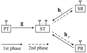
Considering a cognitive relay network where a ST assists to forward the traffic from a PT to a PR, in exchange for serving its own SR in the same frequency, as illustrated in Fig. 1. The ST is equipped with M๐‘€M antennas while other users have a single antenna. We assume that the ST is energy-limited, and thus powered by PT as well as PR and SR to enhance the harvested energy, which is called DWPT scheme in this paper. Assume that the entire communication time slot, which consists of two equal phases, is normalized to be 1.
Refer to caption
Figure 1: Two-phase DWPT scheme in an energy-limited four-node cognitive relay network.

In the first phase, PT transmits information signal xpsubscript๐‘ฅ๐‘x_{p} with power PPโ€‹Tsubscript๐‘ƒ๐‘ƒ๐‘‡P_{PT}. Meanwhile, PR and SR respectively send energy signals xpโ€ฒsuperscriptsubscript๐‘ฅ๐‘โ€ฒx_{p}^{\prime} and xsโ€ฒsuperscriptsubscript๐‘ฅ๐‘ โ€ฒx_{s}^{\prime} with their corresponding power, PPโ€‹Rsubscript๐‘ƒ๐‘ƒ๐‘…P_{PR} and PSโ€‹Rsubscript๐‘ƒ๐‘†๐‘…P_{SR}. Suppose that different signals are statistically independent. The observation at ST is expressed as

๐ฒr=๐ โ€‹xp+๐กpโ€‹xpโ€ฒ+๐กsโ€‹xsโ€ฒ+๐งr,subscript๐ฒ๐‘Ÿ๐ subscript๐‘ฅ๐‘subscript๐ก๐‘subscriptsuperscript๐‘ฅโ€ฒ๐‘subscript๐ก๐‘ subscriptsuperscript๐‘ฅโ€ฒ๐‘ subscript๐ง๐‘Ÿ{{\mathbf{y}}_{r}}={\mathbf{g}}{x_{p}}+{{\mathbf{h}}_{p}}{x^{\prime}_{p}}+{{\mathbf{h}}_{s}}{x^{\prime}_{s}}+{{\mathbf{n}}_{r}}, (1)

where ๐ ๐ \mathbf{g}, ๐กpsubscript๐ก๐‘\mathbf{h}_{p} and ๐กssubscript๐ก๐‘ \mathbf{h}_{s} are Mร—1๐‘€1M\times 1 channel vectors from PT to ST, PR to ST, and SR to ST, respectively; ๐งrโˆผ๐’žโ€‹๐’ฉโ€‹(0,ฯƒr2โ€‹๐ˆM)similar-tosubscript๐ง๐‘Ÿ๐’ž๐’ฉ0superscriptsubscript๐œŽ๐‘Ÿ2subscript๐ˆ๐‘€{{\mathbf{n}}_{r}}\sim{\cal CN}(0,\sigma_{r}^{2}{{\mathbf{I}}_{M}}) is the received noise vector at ST. To concurrently process the information decoding and the energy harvesting, the practical PS receiver architecture is adopted at ST. In particular, the received signal is split into two streams, one for ID and one for EH, with the relative power ratio of ฯ๐œŒ\rho and 1โˆ’ฯ1๐œŒ1-\rho, respectively. The signal stream for EH and the harvested energy at ST are respectively given by

๐ฒrEโ€‹H=1โˆ’ฯโ€‹(๐ โ€‹xp+๐กpโ€‹xpโ€ฒ+๐กsโ€‹xsโ€ฒ+๐งr)โ€‹andsuperscriptsubscript๐ฒ๐‘Ÿ๐ธ๐ป1๐œŒ๐ subscript๐‘ฅ๐‘subscript๐ก๐‘superscriptsubscript๐‘ฅ๐‘โ€ฒsubscript๐ก๐‘ superscriptsubscript๐‘ฅ๐‘ โ€ฒsubscript๐ง๐‘Ÿand{\mathbf{y}}_{r}^{EH}=\sqrt{1-\rho}\left({{\mathbf{g}}{x_{p}}+{{\mathbf{h}}_{p}}{{x}_{p}^{\prime}}+{{\mathbf{h}}_{s}}{{x}_{s}^{\prime}}+{{\mathbf{n}}_{r}}}\right)~{}\text{and} (2)
PrEโ€‹H=ฮพโ€‹(1โˆ’ฯ)โ€‹(PPโ€‹Tโ€‹โ€–๐ โ€–22+PPโ€‹Rโ€‹โ€–๐กpโ€–22+PSโ€‹Rโ€‹โ€–๐กsโ€–22+ฯƒr2),superscriptsubscript๐‘ƒ๐‘Ÿ๐ธ๐ป๐œ‰1๐œŒsubscript๐‘ƒ๐‘ƒ๐‘‡superscriptsubscriptnorm๐ 22subscript๐‘ƒ๐‘ƒ๐‘…superscriptsubscriptnormsubscript๐ก๐‘22subscript๐‘ƒ๐‘†๐‘…superscriptsubscriptnormsubscript๐ก๐‘ 22superscriptsubscript๐œŽ๐‘Ÿ2\displaystyle P_{r}^{EH}\!=\!\xi\left({1-\rho}\right)\!({P_{PT}}\left\|{\mathbf{g}}\right\|_{2}^{2}\!+\!{P_{PR}}\left\|{{{\mathbf{h}}_{p}}}\right\|_{2}^{2}\!+\!{P_{SR}}\left\|{{{\mathbf{h}}_{s}}}\right\|_{2}^{2}\!+\!\sigma_{r}^{2}), (3)

where 0<ฮพโ‰ค10๐œ‰10<\xi\leq 1 is the energy conversion efficiency. Let ๐งcโˆผ๐’žโ€‹๐’ฉโ€‹(0,ฯƒc2โ€‹๐ˆM)similar-tosubscript๐ง๐‘๐’ž๐’ฉ0superscriptsubscript๐œŽ๐‘2subscript๐ˆ๐‘€{{\mathbf{n}}_{c}}\sim{\cal CN}(0,\sigma_{c}^{2}{{\mathbf{I}}_{M}}) denote the Nร—1๐‘1N\times 1 circuit noise vector caused by the signal frequency conversion from RF to baseband and hence the other stream for ID is given by

๐ฒrIโ€‹D=ฯโ€‹(๐ โ€‹xp+๐กpโ€‹xpโ€ฒ+๐กsโ€‹xsโ€ฒ+๐งr)+๐งc.superscriptsubscript๐ฒ๐‘Ÿ๐ผ๐ท๐œŒ๐ subscript๐‘ฅ๐‘subscript๐ก๐‘superscriptsubscript๐‘ฅ๐‘โ€ฒsubscript๐ก๐‘ superscriptsubscript๐‘ฅ๐‘ โ€ฒsubscript๐ง๐‘Ÿsubscript๐ง๐‘{\mathbf{y}}_{r}^{ID}=\sqrt{\rho}\left({{\mathbf{g}}{x_{p}}+{{\mathbf{h}}_{p}}{{x}_{p}^{\prime}}+{{\mathbf{h}}_{s}}{{x}_{s}^{\prime}}+{{\mathbf{n}}_{r}}}\right)+{{\mathbf{n}}_{c}}. (4)

During the second phase, ST uses the AF protocol to relay the traffic from PT to PR and also superimposes its own message xssubscript๐‘ฅ๐‘ x_{s} to SR with Eโ€‹[|xs|2]=1Edelimited-[]superscriptsubscript๐‘ฅ๐‘ 21{\rm E}\left[{{{\left|{{x_{s}}}\right|}^{2}}}\right]=1. Denote ๐…โˆˆโ„‚Mร—M๐…superscriptโ„‚๐‘€๐‘€{\mathbf{F}}\in{\mathbb{C}^{M\times M}} and ๐ฐโˆˆโ„‚Mร—1๐ฐsuperscriptโ„‚๐‘€1{\mathbf{w}}\in{\mathbb{C}^{M\times 1}} as the relay processing matrix and the cognitive beamforming vector respectively, the transmit signal at ST is

๐ฑrsubscript๐ฑ๐‘Ÿ\displaystyle{{\mathbf{x}}_{r}} =๐…๐ฒrIโ€‹D+๐ฐโ€‹xsabsentsuperscriptsubscript๐…๐ฒ๐‘Ÿ๐ผ๐ท๐ฐsubscript๐‘ฅ๐‘ \displaystyle={\mathbf{Fy}}_{r}^{ID}+{\mathbf{w}}{x_{s}}
=๐…โ€‹(ฯโ€‹(๐ โ€‹xp+๐กpโ€‹xpโ€ฒ+๐กsโ€‹xsโ€ฒ+๐งr)+๐งc)+๐ฐโ€‹xsabsent๐…๐œŒ๐ subscript๐‘ฅ๐‘subscript๐ก๐‘superscriptsubscript๐‘ฅ๐‘โ€ฒsubscript๐ก๐‘ superscriptsubscript๐‘ฅ๐‘ โ€ฒsubscript๐ง๐‘Ÿsubscript๐ง๐‘๐ฐsubscript๐‘ฅ๐‘ \displaystyle={\mathbf{F}}\left({\sqrt{\rho}\left({{\mathbf{g}}{x_{p}}+{{\mathbf{h}}_{p}}{{x}_{p}^{\prime}}+{{\mathbf{h}}_{s}}{{x}_{s}^{\prime}}+{{\mathbf{n}}_{r}}}\right)+{{\mathbf{n}}_{c}}}\right)+{\mathbf{w}}{x_{s}} (5)

with average power

PSโ€‹Tโ€‹(๐…,๐ฐ,ฯ)=subscript๐‘ƒ๐‘†๐‘‡๐…๐ฐ๐œŒabsent\displaystyle{P_{ST}}({{\mathbf{F}},{\mathbf{w}},\rho})= ฯ(PPโ€‹Tโˆฅ๐…๐ โˆฅ22+PPโ€‹Rโˆฅ๐…๐กpโˆฅ22+PSโ€‹Rโˆฅ๐…๐กsโˆฅ22\displaystyle\rho\big{(}{P_{PT}}\left\|{{\mathbf{Fg}}}\right\|_{2}^{2}+{P_{PR}}\left\|{{\mathbf{F}}{{\mathbf{h}}_{p}}}\right\|_{2}^{2}+{P_{SR}}\left\|{{\mathbf{F}}{{\mathbf{h}}_{s}}}\right\|_{2}^{2}
+ฯƒr2โˆฅ๐…โˆฅF2)+ฯƒc2โˆฅ๐…โˆฅF2+โˆฅ๐ฐโˆฅ22.\displaystyle+\sigma_{r}^{2}\left\|{\mathbf{F}}\right\|_{F}^{2}\big{)}+\sigma_{c}^{2}\left\|{\mathbf{F}}\right\|_{F}^{2}+\left\|{\mathbf{w}}\right\|_{2}^{2}. (6)

With the perfect CSI at ST, we assume that PR/SR can successfully cancel its self-interference xpโ€ฒsuperscriptsubscript๐‘ฅ๐‘โ€ฒx_{p}^{\prime}/xsโ€ฒsuperscriptsubscript๐‘ฅ๐‘ โ€ฒx_{s}^{\prime}. Hence, the received signals at PR and SR are respectively expressed as

yp=subscript๐‘ฆ๐‘absent\displaystyle{y_{p}}= ฯโ€‹๐กpHโ€‹๐…๐ โ€‹xp+ฯโ€‹๐กpHโ€‹๐…๐กsโ€‹xsโ€ฒ+๐กpHโ€‹๐ฐโ€‹xs๐œŒsuperscriptsubscript๐ก๐‘๐ป๐…๐ subscript๐‘ฅ๐‘๐œŒsuperscriptsubscript๐ก๐‘๐ปsubscript๐…๐ก๐‘ subscriptsuperscript๐‘ฅโ€ฒ๐‘ superscriptsubscript๐ก๐‘๐ป๐ฐsubscript๐‘ฅ๐‘ \displaystyle\sqrt{\rho}{\mathbf{h}}_{p}^{H}{\mathbf{Fg}}{x_{p}}+\sqrt{\rho}{\mathbf{h}}_{p}^{H}{\mathbf{F}}{{\mathbf{h}}_{s}}{x^{\prime}_{s}}+{\mathbf{h}}_{p}^{H}{\mathbf{w}}{x_{s}}
+ฯโ€‹๐กpHโ€‹๐…๐งr+๐กpHโ€‹๐…๐งc+np,๐œŒsuperscriptsubscript๐ก๐‘๐ปsubscript๐…๐ง๐‘Ÿsuperscriptsubscript๐ก๐‘๐ปsubscript๐…๐ง๐‘subscript๐‘›๐‘\displaystyle+\sqrt{\rho}{\mathbf{h}}_{p}^{H}{\mathbf{F}}{{\mathbf{n}}_{r}}+{\mathbf{h}}_{p}^{H}{\mathbf{F}}{{\mathbf{n}}_{c}}+{n_{p}}, (7)
ys=subscript๐‘ฆ๐‘ absent\displaystyle{y_{s}}= ฯโ€‹๐กsHโ€‹๐…๐ โ€‹xp+ฯโ€‹๐กsHโ€‹๐…๐กpโ€‹xpโ€ฒ+๐กsHโ€‹๐ฐโ€‹xs๐œŒsuperscriptsubscript๐ก๐‘ ๐ป๐…๐ subscript๐‘ฅ๐‘๐œŒsuperscriptsubscript๐ก๐‘ ๐ปsubscript๐…๐ก๐‘subscriptsuperscript๐‘ฅโ€ฒ๐‘superscriptsubscript๐ก๐‘ ๐ป๐ฐsubscript๐‘ฅ๐‘ \displaystyle\sqrt{\rho}{\mathbf{h}}_{s}^{H}{\mathbf{Fg}}{x_{p}}+\sqrt{\rho}{\mathbf{h}}_{s}^{H}{\mathbf{F}}{{\mathbf{h}}_{p}}{x^{\prime}_{p}}+\mathbf{h}_{s}^{H}{\mathbf{w}}{x_{s}}
+ฯโ€‹๐กsHโ€‹๐…๐งr+๐กsHโ€‹๐…๐งc+ns,๐œŒsuperscriptsubscript๐ก๐‘ ๐ปsubscript๐…๐ง๐‘Ÿsuperscriptsubscript๐ก๐‘ ๐ปsubscript๐…๐ง๐‘subscript๐‘›๐‘ \displaystyle+\sqrt{\rho}{\mathbf{h}}_{s}^{H}{\mathbf{F}}{{\mathbf{n}}_{r}}+{\mathbf{h}}_{s}^{H}{\mathbf{F}}{{\mathbf{n}}_{c}}+{n_{s}}, (8)

where npโˆผ๐’žโ€‹๐’ฉโ€‹(0,ฯƒp2)similar-tosubscript๐‘›๐‘๐’ž๐’ฉ0superscriptsubscript๐œŽ๐‘2{{{n}}_{p}}\sim{\cal CN}(0,\sigma_{p}^{2}) and nsโˆผ๐’žโ€‹๐’ฉโ€‹(0,ฯƒs2)similar-tosubscript๐‘›๐‘ ๐’ž๐’ฉ0superscriptsubscript๐œŽ๐‘ 2{{{n}}_{s}}\sim{\cal CN}(0,\sigma_{s}^{2}) are additive Gaussian white noises (AWGNs) at PR and SR, respectively. The received signal to interference plus noise ratios (SINRs) at PR and SR are respectively given by

ฮ“pโ€‹(๐…,๐ฐ,ฯ)=subscriptฮ“๐‘๐…๐ฐ๐œŒabsent\displaystyle{\Gamma_{p}}({{\mathbf{F}},{\mathbf{w}},\rho})= (9)
ฯโ€‹PPโ€‹Tโ€‹|๐กpHโ€‹๐…๐ |2ฯโ€‹PSโ€‹Rโ€‹|๐กpHโ€‹๐…๐กs|2+(ฯโ€‹ฯƒr2+ฯƒc2)โ€‹โ€–๐กpHโ€‹๐…โ€–22+|๐กpHโ€‹๐ฐ|2+ฯƒp2,๐œŒsubscript๐‘ƒ๐‘ƒ๐‘‡superscriptsuperscriptsubscript๐ก๐‘๐ป๐…๐ 2๐œŒsubscript๐‘ƒ๐‘†๐‘…superscriptsuperscriptsubscript๐ก๐‘๐ปsubscript๐…๐ก๐‘ 2๐œŒsuperscriptsubscript๐œŽ๐‘Ÿ2superscriptsubscript๐œŽ๐‘2superscriptsubscriptnormsuperscriptsubscript๐ก๐‘๐ป๐…22superscriptsuperscriptsubscript๐ก๐‘๐ป๐ฐ2superscriptsubscript๐œŽ๐‘2\displaystyle\frac{{\rho{P_{PT}}{{\left|{{\mathbf{h}}_{p}^{H}{\mathbf{Fg}}}\right|}^{2}}}}{{\rho{P_{SR}}{{\left|{{\mathbf{h}}_{p}^{H}{\mathbf{F}}{{\mathbf{h}}_{s}}}\right|}^{2}}\!+\!(\rho\sigma_{r}^{2}+\sigma_{c}^{2})\left\|{{\mathbf{h}}_{p}^{H}{\mathbf{F}}}\right\|_{2}^{2}\!+\!\left|{{\mathbf{h}}_{p}^{H}{\mathbf{w}}}\right|^{2}\!+\!\sigma_{p}^{2}}},
ฮ“sโ€‹(๐…,๐ฐ,ฯ)=subscriptฮ“๐‘ ๐…๐ฐ๐œŒabsent\displaystyle{\Gamma_{s}}({{\mathbf{F}},{\mathbf{w}},\rho})= (10)
|๐กsHโ€‹๐ฐ|2ฯโ€‹(PPโ€‹Tโ€‹|๐กsHโ€‹๐…๐ |2+PPโ€‹Rโ€‹|๐กsHโ€‹๐…๐กp|2)+(ฯโ€‹ฯƒr2+ฯƒc2)โ€‹โ€–๐กsHโ€‹๐…โ€–22+ฯƒs2.superscriptsuperscriptsubscript๐ก๐‘ ๐ป๐ฐ2๐œŒsubscript๐‘ƒ๐‘ƒ๐‘‡superscriptsuperscriptsubscript๐ก๐‘ ๐ป๐…๐ 2subscript๐‘ƒ๐‘ƒ๐‘…superscriptsuperscriptsubscript๐ก๐‘ ๐ปsubscript๐…๐ก๐‘2๐œŒsuperscriptsubscript๐œŽ๐‘Ÿ2superscriptsubscript๐œŽ๐‘2superscriptsubscriptnormsuperscriptsubscript๐ก๐‘ ๐ป๐…22superscriptsubscript๐œŽ๐‘ 2\displaystyle\frac{{\left|{{\mathbf{h}}_{s}^{H}{\mathbf{w}}}\right|^{2}}}{{\rho({P_{P\!T}}{{\left|{{\mathbf{h}}_{s}^{H}{\mathbf{Fg}}}\right|}^{2}}\!+\!{P_{P\!R}}{{\left|{{\mathbf{h}}_{s}^{H}{\mathbf{F}}{{\mathbf{h}}_{p}}}\right|}^{2}})\!+\!(\rho\sigma_{r}^{2}\!+\!\sigma_{c}^{2})\!\left\|{{\mathbf{h}}_{s}^{H}{\mathbf{F}}}\right\|_{2}^{2}\!+\!\sigma_{s}^{2}}}.

In this paper, we focus on the joint design of relay matrix ๐…๐…\mathbf{F}, cognitive beamforming vector ๐ฐ๐ฐ\mathbf{w} and power splitter ฯ๐œŒ\rho to maximize the achieved rate of SU, under the constraint that the rate demand of PU, Rpmโ€‹iโ€‹nsuperscriptsubscript๐‘…๐‘๐‘š๐‘–๐‘›{R_{p}^{min}}, is met. The optimization problem is formulated as (๐’ซโ€‹1๐’ซ1\mathcal{P}1)

max๐…,๐ฐ,0โ‰คฯโ‰ค1๐…๐ฐ0๐œŒ1max\displaystyle\underset{{{\mathbf{F}},{\mathbf{w}},0\leq\rho\leq 1}}{\text{max}} ฮ“sโ€‹(๐…,๐ฐ,ฯ)subscriptฮ“๐‘ ๐…๐ฐ๐œŒ\displaystyle\!\!\!\!\!\!\!\!\Gamma_{s}({{\mathbf{F}},{\mathbf{w}},\rho}) (11a)
s. t. ฮ“pโ€‹(๐…,๐ฐ,ฯ)โ‰ฅฮ“pmโ€‹iโ€‹n,subscriptฮ“๐‘๐…๐ฐ๐œŒsuperscriptsubscriptฮ“๐‘๐‘š๐‘–๐‘›\displaystyle\!\!\!\!\!\!\!\!\!\!\!\!\!\!\!\!\Gamma_{p}({{\mathbf{F}},{\mathbf{w}},\rho})\geq\Gamma_{p}^{min}, (11b)
PSโ€‹Tโ€‹(๐…,๐ฐ,ฯ)โ‰คPrEโ€‹H,subscript๐‘ƒ๐‘†๐‘‡๐…๐ฐ๐œŒsuperscriptsubscript๐‘ƒ๐‘Ÿ๐ธ๐ป\displaystyle\!\!\!\!\!\!\!\!\!\!\!\!\!\!\!\!\!\!\!\!\!\!\!\!P_{ST}({{\mathbf{F}},{\mathbf{w}},\rho})\leq P_{r}^{EH}, (11c)

where ฮ“pmโ€‹iโ€‹n=2Rpmโ€‹iโ€‹nโˆ’1superscriptsubscriptฮ“๐‘๐‘š๐‘–๐‘›superscript2superscriptsubscript๐‘…๐‘๐‘š๐‘–๐‘›1\Gamma_{p}^{min}=2^{R_{p}^{min}}-1. Constraint (11c) is to guarantee that the transmission power at ST is not more than its harvested energy.

III Solutions to DWPT with Perfect CSI

In this section, we suppose that all the channel knowledge is perfectly known at ST. Under this assumption, both the optimal and low-complexity suboptimal solutions to problem ๐’ซโ€‹1๐’ซ1\mathcal{P}1 are proposed.

III-A Optimal Solution to DWPT

In this subsection, we present the optimal solution to problem ๐’ซโ€‹1๐’ซ1\mathcal{P}1. Given fixed ฯ๐œŒ\rho, optimal ๐…๐…\mathbf{F} and ๐ฐ๐ฐ\mathbf{w} are obtained, and then the optimal ฯ๐œŒ\rho is found via bisection. In what follows, we first focus on the design of optimal ๐…๐…\mathbf{F} and ๐ฐ๐ฐ\mathbf{w} with fixed ฯ๐œŒ\rho.

Proposition 1: Define two QR decompositions as [๐กs,ย โ€‹๐กp]=๐•1โ€‹๐‘1subscript๐กsย subscript๐กpsubscript๐•1subscript๐‘1\left[{{{\mathbf{h}}_{s}},{\text{ }}{{\mathbf{h}}_{p}}}\right]={{\mathbf{V}}_{1}}{{\mathbf{R}}_{1}} and [๐กs,ย โ€‹๐กp,ย โ€‹๐ ]=๐”2โ€‹๐‘2subscript๐กsย subscript๐กpย ๐ subscript๐”2subscript๐‘2\left[{{{\mathbf{h}}_{s}},{\text{ }}{{\mathbf{h}}_{p}},{\text{ }}{\mathbf{g}}}\right]={{\mathbf{U}}_{2}}{{\mathbf{R}}_{2}}, where ๐•1โˆˆโ„‚Mร—2subscript๐•1superscriptโ„‚M2{{\mathbf{V}}_{1}}\in{\mathbb{C}^{M\times 2}}, ๐”2โˆˆโ„‚Mร—3subscript๐”2superscriptโ„‚M3{{\mathbf{U}}_{2}}\in{\mathbb{C}^{M\times 3}} are orthonormal matrices and ๐‘1โˆˆโ„‚2ร—2subscript๐‘1superscriptโ„‚22{{\mathbf{R}}_{1}}\in{\mathbb{C}^{2\times 2}}, ๐‘2โˆˆโ„‚3ร—3subscript๐‘2superscriptโ„‚33{{\mathbf{R}}_{2}}\in{\mathbb{C}^{3\times 3}} are upper triangular matrices. Then, the optimal relay matrix and cognitive beamforming vector have the following structures:

๐…โ€‹ย =๐•1โ€‹๐€๐”2H,๐ฐโ€‹ย =๐•1โ€‹๐›,formulae-sequence๐…ย subscript๐•1superscriptsubscript๐€๐”2๐ป๐ฐย subscript๐•1๐›{\mathbf{F}}{\text{ }}={{\mathbf{V}}_{1}}{\mathbf{AU}}_{2}^{H},~{}~{}{\mathbf{w}}{\text{ }}={{\mathbf{V}}_{1}}{\mathbf{b}}, (12)

where ๐€โˆˆโ„‚2ร—3๐€superscriptโ„‚23{\mathbf{A}}\in{\mathbb{C}^{2\times 3}} and ๐›โˆˆโ„‚2ร—1๐›superscriptโ„‚21{\mathbf{b}}\in{\mathbb{C}^{2\times 1}} are optimization variables.

Proof: Please see Appendix A. โˆŽ

If Mโ‰ฅ3๐‘€3M\geq 3, with Proposition 1, the M2superscript๐‘€2M^{2} unknowns in ๐…๐…\mathbf{F} and M๐‘€M unknowns in ๐ฐ๐ฐ\mathbf{w} are respectively reduced to 2ร—3232\times 3 unknowns and 222 unknowns. This greatly reduces the computational complexity of the beamforming design. If Mโ‰ค2๐‘€2M\leq 2, we optimize ๐…๐…\mathbf{F} and ๐ฐ๐ฐ\mathbf{w} directly.

Define ๐ก^s=๐•1Hโ€‹๐กssubscript^๐ก๐‘ superscriptsubscript๐•1๐ปsubscript๐ก๐‘ {{\mathbf{\hat{h}}}_{s}}={\mathbf{V}}_{1}^{H}{{\mathbf{h}}_{s}}, ๐ก^p=๐•1Hโ€‹๐กpsubscript^๐ก๐‘superscriptsubscript๐•1๐ปsubscript๐ก๐‘{{\mathbf{\hat{h}}}_{p}}={\mathbf{V}}_{1}^{H}{{\mathbf{h}}_{p}}, ๐กยฏs=๐”2Hโ€‹๐กssubscriptยฏ๐ก๐‘ superscriptsubscript๐”2๐ปsubscript๐ก๐‘ {{\mathbf{\bar{h}}}_{s}}={\mathbf{U}}_{2}^{H}{{\mathbf{h}}_{s}}, ๐กยฏp=๐”2Hโ€‹๐กpsubscriptยฏ๐ก๐‘superscriptsubscript๐”2๐ปsubscript๐ก๐‘{{\mathbf{\bar{h}}}_{p}}={\mathbf{U}}_{2}^{H}{{\mathbf{h}}_{p}} and ๐ ยฏ=๐”2Hโ€‹๐ ยฏ๐ superscriptsubscript๐”2๐ป๐ {\mathbf{\bar{g}}}={\mathbf{U}}_{2}^{H}{\mathbf{g}}, with Proposition 1, the problem ๐’ซโ€‹1๐’ซ1\mathcal{P}1 can be reformulated as (given fixed ฯ๐œŒ\rho) (๐’ซโ€‹2๐’ซ2\mathcal{P}2)

max๐€,๐›๐€๐›max\displaystyle\!\!\underset{{{\mathbf{A}},{\mathbf{b}}}}{\text{max}} |๐ก^sHโ€‹๐›|2ฯโ€‹(PPโ€‹Tโ€‹|๐ก^sHโ€‹๐€โ€‹๐ ยฏ|2+PPโ€‹Rโ€‹|๐ก^sHโ€‹๐€โ€‹๐กยฏp|2)+(ฯโ€‹ฯƒr2+ฯƒc2)โ€‹โ€–๐ก^sHโ€‹๐€โ€–22+ฯƒs2superscriptsuperscriptsubscript^๐ก๐‘ ๐ป๐›2๐œŒsubscript๐‘ƒ๐‘ƒ๐‘‡superscriptsuperscriptsubscript^๐ก๐‘ ๐ป๐€ยฏ๐ 2subscript๐‘ƒ๐‘ƒ๐‘…superscriptsuperscriptsubscript^๐ก๐‘ ๐ป๐€subscriptยฏ๐ก๐‘2๐œŒsuperscriptsubscript๐œŽ๐‘Ÿ2superscriptsubscript๐œŽ๐‘2superscriptsubscriptnormsuperscriptsubscript^๐ก๐‘ ๐ป๐€22superscriptsubscript๐œŽ๐‘ 2\displaystyle\!\!\!\!\frac{{\left|{{\mathbf{\hat{h}}}_{s}^{H}{\mathbf{b}}}\right|^{2}}}{{\rho\big{(}{P_{P\!T}}{{\left|{{\mathbf{\hat{h}}}_{s}^{H}{\mathbf{A\bar{g}}}}\right|}^{2}}\!\!+\!\!{P_{P\!R}}{{\left|{{\mathbf{\hat{h}}}_{s}^{H}{\mathbf{A}}{{{\mathbf{\bar{h}}}}_{p}}}\right|}^{2}}\big{)}\!\!+\!\!(\rho\sigma_{r}^{2}\!\!+\!\!\sigma_{c}^{2})\!\left\|{{\mathbf{\hat{h}}}_{s}^{H}{\mathbf{A}}}\right\|_{2}^{2}\!\!+\!\!\sigma_{s}^{2}}} (13a)
s. t. ฯโ€‹PPโ€‹Tโ€‹|๐ก^pHโ€‹๐€โ€‹๐ ยฏ|2ฯโ€‹PSโ€‹Rโ€‹|๐ก^pHโ€‹๐€โ€‹๐กยฏs|2+(ฯโ€‹ฯƒr2+ฯƒc2)โ€‹โ€–๐ก^pHโ€‹๐€โ€–22+|๐ก^pHโ€‹๐›|2+ฯƒp2โ‰ฅฮ“pmin,๐œŒsubscript๐‘ƒ๐‘ƒ๐‘‡superscriptsuperscriptsubscript^๐ก๐‘๐ป๐€ยฏ๐ 2๐œŒsubscript๐‘ƒ๐‘†๐‘…superscriptsuperscriptsubscript^๐ก๐‘๐ป๐€subscriptยฏ๐ก๐‘ 2๐œŒsuperscriptsubscript๐œŽ๐‘Ÿ2superscriptsubscript๐œŽ๐‘2superscriptsubscriptnormsuperscriptsubscript^๐ก๐‘๐ป๐€22superscriptsuperscriptsubscript^๐ก๐‘๐ป๐›2superscriptsubscript๐œŽ๐‘2superscriptsubscriptฮ“๐‘\displaystyle\!\!\!\!\!\frac{{\rho{P_{PT}}{{\left|{{\mathbf{\hat{h}}}_{p}^{H}{\mathbf{A\bar{g}}}}\right|}^{2}}}}{{\rho{P_{SR}}{{\left|{{\mathbf{\hat{h}}}_{p}^{H}{\mathbf{A}}{{{\mathbf{\bar{h}}}}_{s}}}\right|}^{2}}\!\!+\!\!(\rho\sigma_{r}^{2}\!\!+\!\!\sigma_{c}^{2})\!\left\|{{\mathbf{\hat{h}}}_{p}^{H}{\mathbf{A}}}\right\|_{2}^{2}\!\!+\!\!\left|{{\mathbf{\hat{h}}}_{p}^{H}{\mathbf{b}}}\right|^{2}\!\!+\!\!\sigma_{p}^{2}}}\!\!\geq\!\!\Gamma_{p}^{\min}, (13b)
ฯโ€‹(PPโ€‹Tโ€‹โ€–๐€โ€‹๐ ยฏโ€–22+PPโ€‹Rโ€‹โ€–๐€โ€‹๐กยฏpโ€–22+PSโ€‹Rโ€‹โ€–๐€โ€‹๐กยฏsโ€–22)๐œŒsubscript๐‘ƒ๐‘ƒ๐‘‡superscriptsubscriptnorm๐€ยฏ๐ 22subscript๐‘ƒ๐‘ƒ๐‘…superscriptsubscriptnorm๐€subscriptยฏ๐ก๐‘22subscript๐‘ƒ๐‘†๐‘…superscriptsubscriptnorm๐€subscriptยฏ๐ก๐‘ 22\displaystyle\!\!\!\!\rho({P_{PT}}\left\|{{\mathbf{A\bar{g}}}}\right\|_{2}^{2}+{P_{PR}}\left\|{{\mathbf{A}}{{{\mathbf{\bar{h}}}}_{p}}}\right\|_{2}^{2}+{P_{SR}}\left\|{{\mathbf{A}}{{{\mathbf{\bar{h}}}}_{s}}}\right\|_{2}^{2})
+(ฯโ€‹ฯƒr2+ฯƒc2)โ€‹โ€–๐€โ€–F2+โ€–๐›โ€–22โ‰คPrEโ€‹H.๐œŒsuperscriptsubscript๐œŽ๐‘Ÿ2superscriptsubscript๐œŽ๐‘2superscriptsubscriptnorm๐€๐น2superscriptsubscriptnorm๐›22superscriptsubscript๐‘ƒ๐‘Ÿ๐ธ๐ป\displaystyle+(\rho\sigma_{r}^{2}+\sigma_{c}^{2})\left\|{\mathbf{A}}\right\|_{F}^{2}+\left\|{\mathbf{b}}\right\|_{2}^{2}\leq P_{r}^{EH}. (13c)

To solve this problem effectively, we use equations

vecโก(๐€๐—๐)=(๐TโŠ—๐€)โ€‹vecโก(๐—)โ€‹andvec๐€๐—๐tensor-productsuperscript๐๐‘‡๐€vec๐—and\operatorname{vec}({\mathbf{AXB}})=({{\mathbf{B}}^{T}}\otimes{\mathbf{A}})\operatorname{vec}({\mathbf{X}})~{}\text{and} (14)
๐“๐ซโ€‹(๐—1Tโ€‹๐—2)=๐ฏ๐ž๐œโ€‹(๐—1)Tโ€‹๐ฏ๐ž๐œโ€‹(๐—2)๐“๐ซsuperscriptsubscript๐—1๐‘‡subscript๐—2๐ฏ๐ž๐œsuperscriptsubscript๐—1๐‘‡๐ฏ๐ž๐œsubscript๐—2{\mathbf{Tr}}({\mathbf{X}}_{1}^{T}{{\mathbf{X}}_{2}})={\mathbf{vec}}{({{\mathbf{X}}_{1}})^{T}}{\mathbf{vec}}({{\mathbf{X}}_{2}}) (15)

to further rewritten problem ๐’ซโ€‹2๐’ซ2\mathcal{P}2 as (๐’ซโ€‹2.1๐’ซ2.1\mathcal{P}2.1)

max๐š,๐›๐š๐›max\displaystyle\!\!\!\!\!\underset{{{\mathbf{a}},{\mathbf{b}}}}{\text{max}} ๐›Hโ€‹๐‡^sโ€‹๐›๐šHโ€‹๐ฯโ€‹๐š+ฯƒs2superscript๐›๐ปsubscript^๐‡๐‘ ๐›superscript๐š๐ปsubscript๐๐œŒ๐šsuperscriptsubscript๐œŽ๐‘ 2\displaystyle\frac{{{{\mathbf{b}}^{H}}{{{\mathbf{\hat{H}}}}_{s}}{\mathbf{b}}}}{{{{\mathbf{a}}^{H}}{{\mathbf{B}}_{\rho}}{\mathbf{a}}+\sigma_{s}^{2}}} (16a)
s. t. ๐šHโ€‹๐‚ฯโ€‹๐š๐šHโ€‹๐ƒฯโ€‹๐š+๐›Hโ€‹๐‡^pโ€‹๐›+ฯƒp2โ‰ฅฮ“pmin,superscript๐š๐ปsubscript๐‚๐œŒ๐šsuperscript๐š๐ปsubscript๐ƒ๐œŒ๐šsuperscript๐›๐ปsubscript^๐‡๐‘๐›superscriptsubscript๐œŽ๐‘2superscriptsubscriptฮ“๐‘\displaystyle\!\!\!\!\!\!\!\frac{{{{\mathbf{a}}^{H}}{{\mathbf{C}}_{\rho}}{\mathbf{a}}}}{{{{\mathbf{a}}^{H}}{{\mathbf{D}}_{\rho}}{\mathbf{a}}+{{\mathbf{b}}^{H}}{{{\mathbf{\hat{H}}}}_{p}}{\mathbf{b}}+\sigma_{p}^{2}}}\geq\!\!\Gamma_{p}^{\min}, (16b)
๐šHโ€‹๐„ฯโ€‹๐š+๐›Hโ€‹๐›โ‰คPrEโ€‹H,superscript๐š๐ปsubscript๐„๐œŒ๐šsuperscript๐›๐ป๐›superscriptsubscript๐‘ƒ๐‘Ÿ๐ธ๐ป\displaystyle{{\mathbf{a}}^{H}}{{\mathbf{E}}_{\rho}}{\mathbf{a}}+{{\mathbf{b}}^{H}}{\mathbf{b}}\leq P_{r}^{EH}, (16c)

where

๐ฯ=ฯโ€‹(ฯƒr2โ€‹๐ˆ+PPโ€‹Tโ€‹๐†ยฏT+PPโ€‹Rโ€‹๐‡ยฏpT)โŠ—๐‡^s+ฯƒc2โ€‹๐ˆโŠ—๐‡^s,subscript๐๐œŒtensor-product๐œŒsuperscriptsubscript๐œŽ๐‘Ÿ2๐ˆsubscript๐‘ƒ๐‘ƒ๐‘‡superscriptยฏ๐†๐‘‡subscript๐‘ƒ๐‘ƒ๐‘…superscriptsubscriptยฏ๐‡๐‘๐‘‡subscript^๐‡๐‘ tensor-productsuperscriptsubscript๐œŽ๐‘2๐ˆsubscript^๐‡๐‘ {{\mathbf{B}}_{\rho}}=\rho\left({\sigma_{r}^{2}{\mathbf{I}}+{P_{PT}}{{{\mathbf{\bar{G}}}}^{T}}+{P_{PR}}{\mathbf{\bar{H}}}_{p}^{T}}\right)\otimes{{{\mathbf{\hat{H}}}}_{s}}+\sigma_{c}^{2}{\mathbf{I}}\otimes{{{\mathbf{\hat{H}}}}_{s}}, (17)
๐‚ฯ=ฯโ€‹PPโ€‹Tโ€‹๐†ยฏTโŠ—๐‡^p,subscript๐‚๐œŒtensor-product๐œŒsubscript๐‘ƒ๐‘ƒ๐‘‡superscriptยฏ๐†๐‘‡subscript^๐‡๐‘{{\mathbf{C}}_{\rho}}=\rho{P_{PT}}{{\mathbf{\bar{G}}}^{T}}\otimes{{\mathbf{\hat{H}}}_{p}}, (18)
๐ƒฯ=ฯโ€‹(ฯƒr2โ€‹๐ˆ+PSโ€‹Rโ€‹๐‡ยฏsT)โŠ—๐‡^p+ฯƒc2โ€‹๐ˆโŠ—๐‡^p,subscript๐ƒ๐œŒtensor-product๐œŒsuperscriptsubscript๐œŽ๐‘Ÿ2๐ˆsubscript๐‘ƒ๐‘†๐‘…superscriptsubscriptยฏ๐‡๐‘ ๐‘‡subscript^๐‡๐‘tensor-productsuperscriptsubscript๐œŽ๐‘2๐ˆsubscript^๐‡๐‘{{\mathbf{D}}_{\rho}}=\rho\left({\sigma_{r}^{2}{\mathbf{I}}+{P_{SR}}{\mathbf{\bar{H}}}_{s}^{T}}\right)\otimes{{{\mathbf{\hat{H}}}}_{p}}+\sigma_{c}^{2}{\mathbf{I}}\otimes{{{\mathbf{\hat{H}}}}_{p}}, (19)
๐„ฯ=subscript๐„๐œŒabsent\displaystyle{{\mathbf{E}}_{\rho}}= ฯ((PPโ€‹T๐†ยฏT+PPโ€‹R๐‡ยฏpT+PSโ€‹R๐‡ยฏsT)โŠ—๐ˆ2ร—2\displaystyle\rho\big{(}({P_{PT}}{{{\mathbf{\bar{G}}}}^{T}}+{P_{PR}}{\mathbf{\bar{H}}}_{p}^{T}+{P_{SR}}{\mathbf{\bar{H}}}_{s}^{T})\otimes{{\mathbf{I}}_{2\times 2}} (20)
+ฯƒr2๐ˆ6ร—6)+ฯƒc2๐ˆ6ร—6,and\displaystyle+\sigma_{r}^{2}{{\mathbf{I}}_{6\times 6}}\big{)}+\sigma_{c}^{2}{{\mathbf{I}}_{6\times 6}},~{}\text{and}
๐š=vecโก(๐€),๐‡^s=๐ก^sโ€‹๐ก^sH,๐‡^p=๐ก^pโ€‹๐ก^pH,formulae-sequence๐švec๐€formulae-sequencesubscript^๐‡๐‘ subscript^๐ก๐‘ superscriptsubscript^๐ก๐‘ ๐ปsubscript^๐‡๐‘subscript^๐ก๐‘superscriptsubscript^๐ก๐‘๐ป{\mathbf{a}}=\operatorname{vec}({\mathbf{A}}),{{\mathbf{\hat{H}}}_{s}}={{\mathbf{\hat{h}}}_{s}}{\mathbf{\hat{h}}}_{s}^{H},{{\mathbf{\hat{H}}}_{p}}={{\mathbf{\hat{h}}}_{p}}{\mathbf{\hat{h}}}_{p}^{H}, (21)
๐‡ยฏs=๐กยฏsโ€‹๐กยฏsH,๐‡ยฏp=๐กยฏpโ€‹๐กยฏpH,๐†ยฏ=๐ ยฏโ€‹๐ ยฏH.formulae-sequencesubscriptยฏ๐‡๐‘ subscriptยฏ๐ก๐‘ superscriptsubscriptยฏ๐ก๐‘ ๐ปformulae-sequencesubscriptยฏ๐‡๐‘subscriptยฏ๐ก๐‘superscriptsubscriptยฏ๐ก๐‘๐ปยฏ๐†ยฏ๐ superscriptยฏ๐ ๐ป{{\mathbf{\bar{H}}}_{s}}={{\mathbf{\bar{h}}}_{s}}{\mathbf{\bar{h}}}_{s}^{H},{{\mathbf{\bar{H}}}_{p}}={{\mathbf{\bar{h}}}_{p}}{\mathbf{\bar{h}}}_{p}^{H},{\mathbf{\bar{G}}}={\mathbf{\bar{g}}}{{\mathbf{\bar{g}}}^{H}}. (22)

Before solving problem ๐’ซ๐’ซ\mathcal{P}2.1, we first analyze its feasible condition, which can be obtained by finding the maximum ฮ“pmโ€‹iโ€‹nโฃโˆ—superscriptsubscriptฮ“๐‘๐‘š๐‘–๐‘›\Gamma_{p}^{min*}. Setting ๐›=๐ŸŽ๐›0\mathbf{b}=\mathbf{0}, the optimization problem is given as (๐’ซโ€‹2.2๐’ซ2.2\mathcal{P}2.2)

max๐š๐šmax\displaystyle\underset{{{\mathbf{a}}}}{\text{max}} ๐šHโ€‹๐‚ฯโ€‹๐š๐šHโ€‹๐ƒฯโ€‹๐š+ฯƒp2superscript๐š๐ปsubscript๐‚๐œŒ๐šsuperscript๐š๐ปsubscript๐ƒ๐œŒ๐šsuperscriptsubscript๐œŽ๐‘2\displaystyle\!\!\!\!\!\!\!\!\!\!\!\!\!\!\!\!\!\!\!\!\!\!\!\!\!\!\!\!\!\!\!\!\!\!\!\frac{{{{\mathbf{a}}^{H}}{{\mathbf{C}}_{\rho}}{\mathbf{a}}}}{{{{\mathbf{a}}^{H}}{{\mathbf{D}}_{\rho}}{\mathbf{a}}+\sigma_{p}^{2}}} (23a)
s. t. ๐šHโ€‹๐„ฯโ€‹๐šโ‰คPrEโ€‹H.superscript๐š๐ปsubscript๐„๐œŒ๐šsuperscriptsubscript๐‘ƒ๐‘Ÿ๐ธ๐ป\displaystyle\!\!\!\!\!\!\!\!\!\!\!\!\!\!\!\!\!\!\!\!\!\!\!\!\!\!\!\!\!\!\!\!\!\!\!{{\mathbf{a}}^{H}}{{\mathbf{E}}_{\rho}}{\mathbf{a}}\leq P_{r}^{EH}. (23b)

It is easy to verify that, at the optimum, the power constraint (23b) is active, i.e., ๐šHโ€‹๐„ฯโ€‹๐š=PrEโ€‹Hsuperscript๐š๐ปsubscript๐„๐œŒ๐šsuperscriptsubscript๐‘ƒ๐‘Ÿ๐ธ๐ป{{\mathbf{a}}^{H}}{{\mathbf{E}}_{\rho}}{\mathbf{a}}=P_{r}^{EH}. With this equation, problem ๐’ซโ€‹2.2๐’ซ2.2\mathcal{P}2.2 can be equivalently written as (๐’ซ๐’ซ\mathcal{P}2.3)

maxโ€–๐šโ€–22=1โ€‹๐šHโ€‹๐‚ฯโ€‹๐š๐šHโ€‹(๐ƒฯ+ฯƒp2โ€‹/โ€‹PrEโ€‹Hโ€‹๐„ฯ)โ€‹๐šsuperscriptsubscriptnorm๐š221maxsuperscript๐š๐ปsubscript๐‚๐œŒ๐šsuperscript๐š๐ปsubscript๐ƒ๐œŒsuperscriptsubscript๐œŽ๐‘2/superscriptsubscript๐‘ƒ๐‘Ÿ๐ธ๐ปsubscript๐„๐œŒ๐š\underset{{{\left\|{\mathbf{a}}\right\|_{2}^{2}}=1}}{\text{max}}~{}~{}\frac{{{{\mathbf{a}}^{H}}{{\mathbf{C}}_{\rho}}{\mathbf{a}}}}{{{{\mathbf{a}}^{H}}\big{(}{{\mathbf{D}}_{\rho}}+{{\sigma_{p}^{2}}\mathord{\left/{\vphantom{{\sigma_{p}^{2}}{P_{r}^{EH}}}}\right.\kern-1.2pt}{P_{r}^{EH}}}{{\mathbf{E}}_{\rho}}\big{)}{\mathbf{a}}}} (24)

which is a generalized Rayleigh quotient [13]. The optimal ๐šโˆ—superscript๐š\mathbf{a}^{*} of problem ๐’ซโ€‹2.3๐’ซ2.3\mathcal{P}2.3 is equal to the dominant generalized eigenvector of the matrix pair (๐‚ฯ,๐ƒฯ+ฯƒp2โ€‹/โ€‹PrEโ€‹Hโ€‹๐„ฯ)subscript๐‚๐œŒsubscript๐ƒ๐œŒsuperscriptsubscript๐œŽ๐‘2/superscriptsubscript๐‘ƒ๐‘Ÿ๐ธ๐ปsubscript๐„๐œŒ\big{(}{{\mathbf{C}}_{\rho}},~{}{{\mathbf{D}}_{\rho}}+{{\sigma_{p}^{2}}\mathord{\left/{\vphantom{{\sigma_{p}^{2}}{P_{r}^{EH}}}}\right.\kern-1.2pt}{P_{r}^{EH}}}{{\mathbf{E}}_{\rho}}\big{)}. And the achieved optimal value of problem ๐’ซโ€‹2.3๐’ซ2.3\mathcal{P}2.3, ฮ“pmโ€‹iโ€‹nโฃโˆ—superscriptsubscriptฮ“๐‘๐‘š๐‘–๐‘›\Gamma_{p}^{min*}, is the largest generalized eigenvalue of the same matrix pair. Thus, the feasible condition is ฮ“pmโ€‹iโ€‹nโ‰คฮ“pmโ€‹iโ€‹nโฃโˆ—superscriptsubscriptฮ“๐‘๐‘š๐‘–๐‘›superscriptsubscriptฮ“๐‘๐‘š๐‘–๐‘›\Gamma_{p}^{min}\leq\Gamma_{p}^{min*}.

Within the feasible region, we then resort to the SDR technique and Charnes-Cooper transformation [14] to solve problem ๐’ซโ€‹2.1๐’ซ2.1\mathcal{P}2.1. Introducing ๐€ยฏ=๐š๐šH,๐ยฏ=๐›๐›Hformulae-sequenceยฏ๐€superscript๐š๐š๐ปยฏ๐superscript๐›๐›๐ป{\mathbf{\bar{A}}}={\mathbf{a}}{{\mathbf{a}}^{H}},{\mathbf{\bar{B}}}={\mathbf{b}}{{\mathbf{b}}^{H}} and applying SDR technique, problem ๐’ซโ€‹2.1๐’ซ2.1\mathcal{P}2.1 can be relaxed as (๐’ซ๐’ซ\mathcal{P}2.4)

max๐€ยฏ,๐ยฏยฏ๐€ยฏ๐max\displaystyle\underset{{{\mathbf{\bar{A}}},{\mathbf{\bar{B}}}}}{\text{max}} Trโก(๐‡^sโ€‹๐ยฏ)Trโก(๐ฯโ€‹๐€ยฏ)+ฯƒs2Trsubscript^๐‡๐‘ ยฏ๐Trsubscript๐๐œŒยฏ๐€superscriptsubscript๐œŽ๐‘ 2\displaystyle\frac{{\operatorname{Tr}\left({{{{\mathbf{\hat{H}}}}_{s}}{\mathbf{\bar{B}}}}\right)}}{{\operatorname{Tr}\left({{{\mathbf{B}}_{\rho}}{\mathbf{\bar{A}}}}\right)+\sigma_{s}^{2}}} (25a)
s. t. Trโก(๐‚ฯโ€‹๐€ยฏ)โˆ’ฮ“pminโ€‹(Trโก(๐ƒฯโ€‹๐€ยฏ)+Trโก(๐‡^pโ€‹๐ยฏ))โ‰ฅฮ“pminโ€‹ฯƒp2,Trsubscript๐‚๐œŒยฏ๐€superscriptsubscriptฮ“๐‘Trsubscript๐ƒ๐œŒยฏ๐€Trsubscript^๐‡๐‘ยฏ๐superscriptsubscriptฮ“๐‘superscriptsubscript๐œŽ๐‘2\displaystyle\!\!\!\!\operatorname{Tr}\left({{{\mathbf{C}}_{\rho}}{\mathbf{\bar{A}}}}\right)\!-\!\Gamma_{p}^{\min}\left({\operatorname{Tr}\left({{{\mathbf{D}}_{\rho}}{\mathbf{\bar{A}}}}\right)\!+\!\operatorname{Tr}({{{{\mathbf{\hat{H}}}}_{p}}{\mathbf{\bar{B}}}})}\right)\!\geq\!\Gamma_{p}^{\min}\sigma_{p}^{2}, (25b)
Trโก(๐„ฯโ€‹๐€ยฏ)+Trโก(๐ยฏ)โ‰คPrEโ€‹H,Trsubscript๐„๐œŒยฏ๐€Trยฏ๐superscriptsubscript๐‘ƒ๐‘Ÿ๐ธ๐ป\displaystyle\operatorname{Tr}\left({{{\mathbf{E}}_{\rho}}{\mathbf{\bar{A}}}}\right)+\operatorname{Tr}\left({{\mathbf{\bar{B}}}}\right)\leq P_{r}^{EH}, (25c)
๐€ยฏโชฐ๐ŸŽ,๐ยฏโชฐ๐ŸŽ,formulae-sequencesucceeds-or-equalsยฏ๐€0succeeds-or-equalsยฏ๐0\displaystyle{\mathbf{\bar{A}}}\succeq{\mathbf{0}},{\mathbf{\bar{B}}}\succeq{\mathbf{0}}, (25d)

which is a linear fractional quasi-convex problem. From Charnes-Cooper transformation, we define ๐€^=qโ€‹๐€ยฏ^๐€๐‘žยฏ๐€{\mathbf{\hat{A}}}=q{\mathbf{\bar{A}}}, ๐^=qโ€‹๐ยฏโ€‹(q>0)^๐๐‘žยฏ๐๐‘ž0{\mathbf{\hat{B}}}=q{\mathbf{\bar{B}}}(q>0) and rewrite the problem ๐’ซโ€‹2.4๐’ซ2.4\mathcal{P}2.4 as (๐’ซโ€‹2.5๐’ซ2.5\mathcal{P}2.5)

max๐€^,๐^,q^๐€^๐๐‘žmax\displaystyle\underset{{{\mathbf{\hat{A}}},{\mathbf{\hat{B}}},q}}{\text{max}} Trโก(๐‡^sโ€‹๐^)Trsubscript^๐‡๐‘ ^๐\displaystyle\operatorname{Tr}\left({{{{\mathbf{\hat{H}}}}_{s}}{\mathbf{\hat{B}}}}\right) (26a)
s. t. Trโก(๐ฯโ€‹๐€^)+ฯƒs2โ€‹q=1,Trsubscript๐๐œŒ^๐€superscriptsubscript๐œŽ๐‘ 2๐‘ž1\displaystyle\operatorname{Tr}\left({{{\mathbf{B}}_{\rho}}{\mathbf{\hat{A}}}}\right)+\sigma_{s}^{2}q=1, (26b)
Trโก(๐‚ฯโ€‹๐€^)โˆ’ฮ“pminโ€‹(Trโก(๐ƒฯโ€‹๐€^)+Trโก(๐‡^pโ€‹๐^))โ‰ฅฮ“pminโ€‹ฯƒp2โ€‹q,Trsubscript๐‚๐œŒ^๐€superscriptsubscriptฮ“๐‘Trsubscript๐ƒ๐œŒ^๐€Trsubscript^๐‡๐‘^๐superscriptsubscriptฮ“๐‘superscriptsubscript๐œŽ๐‘2๐‘ž\displaystyle\!\!\!\!\!\!\!\!\!\!\!\!\!\!\!\!\!\!\!\!\!\!\!\operatorname{Tr}\left({{{\mathbf{C}}_{\rho}}{\mathbf{\hat{A}}}}\right)\!-\!\Gamma_{p}^{\min}\left({\operatorname{Tr}({{{\mathbf{D}}_{\rho}}{\mathbf{\hat{A}}}})\!+\!\operatorname{Tr}({{{{\mathbf{\hat{H}}}}_{p}}{\mathbf{\hat{B}}}})}\right)\!\geq\!\Gamma_{p}^{\min}\sigma_{p}^{2}q,\! (26c)
Trโก(๐„ฯโ€‹๐€^)+Trโก(๐^)โ‰คPrEโ€‹Hโ€‹q,Trsubscript๐„๐œŒ^๐€Tr^๐superscriptsubscript๐‘ƒ๐‘Ÿ๐ธ๐ป๐‘ž\displaystyle\operatorname{Tr}\left({{{\mathbf{E}}_{\rho}}{\mathbf{\hat{A}}}}\right)+\operatorname{Tr}\left({{\mathbf{\hat{B}}}}\right)\leq P_{r}^{EH}q, (26d)
๐€^โชฐ๐ŸŽ,๐^โชฐ๐ŸŽ,q>0,formulae-sequencesucceeds-or-equals^๐€0formulae-sequencesucceeds-or-equals^๐0๐‘ž0\displaystyle{\mathbf{\hat{A}}}\succeq{\mathbf{0}},{\mathbf{\hat{B}}}\succeq{\mathbf{0}},q>0, (26e)

which is a convex SDP and can be efficiently solved by convex optimization solvers, e.g., CVX [15].

Remark 1: More importantly, According to the Theorem 2.3 in [16], the optimal solution to problem ๐’ซ๐’ซ\mathcal{P}2.5 always satisfies Rank2โก(๐€^โˆ—)+Rank2โก(๐^โˆ—)โ‰ค3superscriptRank2superscript^๐€superscriptRank2superscript^๐3{\operatorname{Rank}^{2}}({{\mathbf{\hat{A}}}^{*}})+{\operatorname{Rank}^{2}}({{\mathbf{\hat{B}}}^{*}})\leq 3, since the number of generalized constraints is 3. For the nontrivial case where ๐€^โˆ—โ‰ ๐ŸŽsuperscript^๐€0{{\mathbf{\hat{A}}}^{*}}\neq{\mathbf{0}}, ๐^โˆ—โ‰ ๐ŸŽsuperscript^๐0{{\mathbf{\hat{B}}}^{*}}\neq{\mathbf{0}}, we have Rankโก(๐€^โˆ—)=1Ranksuperscript^๐€1\operatorname{Rank}({{\mathbf{\hat{A}}}^{*}})=1, Rankโก(๐^โˆ—)=1Ranksuperscript^๐1\operatorname{Rank}({{\mathbf{\hat{B}}}^{*}})=1. So the SDR problem is tight and thus the optimal ๐šโˆ—superscript๐š\mathbf{a}^{*} and ๐›โˆ—superscript๐›\mathbf{b}^{*} for problem ๐’ซโ€‹2.1๐’ซ2.1\mathcal{P}2.1 can be obtained.

So far, the optimal solution to problem ๐’ซโ€‹1๐’ซ1\mathcal{P}1 with fixed ฯ๐œŒ\rho is derived. In the sequel, we focus on the finding of optimal ฯ๐œŒ\rho.

Proposition 2: Define the objective value of problem ๐’ซโ€‹2.5๐’ซ2.5\mathcal{P}2.5 as a function of ฯฯ\rho, i.e., hโ€‹(ฯ)hฯh(\rho). Then, hโ€‹(ฯ)hฯh(\rho) is concave in ฯฯ\rho and its optimal value can be obtained via bisection.

Proof: Let ฮธ1subscript๐œƒ1\theta_{1}, ฮธ2subscript๐œƒ2\theta_{2} and ฮธ3subscript๐œƒ3\theta_{3} denote the dual variables of the corresponding constraints in problem ๐’ซ๐’ซ\mathcal{P}2.5, respectively. Then the Lagrangian function of problem ๐’ซ๐’ซ\mathcal{P}2.5 is given by

โ„’โ€‹(๐€^,๐^,q,ฮธ1,ฮธ2,ฮธ3,ฯ)โ€‹ย =Trโก(๐1โ€‹๐€^)+Trโก(๐2โ€‹๐^)+q3,โ„’^๐€^๐๐‘žsubscript๐œƒ1subscript๐œƒ2subscript๐œƒ3๐œŒย Trsubscript๐1^๐€Trsubscript๐2^๐subscript๐‘ž3{\mathcal{L}}\left({{\mathbf{\hat{A}}},{\mathbf{\hat{B}}},q,{\theta_{1}},{\theta_{2}},{\theta_{3}},\rho}\right){\text{ }}=\operatorname{Tr}\left({{{\mathbf{Q}}_{1}}{\mathbf{\hat{A}}}}\right)+\operatorname{Tr}\left({{{\mathbf{Q}}_{2}}{\mathbf{\hat{B}}}}\right)+{q_{3}}, (27)

where

๐1=โˆ’ฮธ1โ€‹๐ฯ+ฮธ2โ€‹๐‚ฯโˆ’ฮธ2โ€‹ฮ“pminโ€‹๐ƒฯโˆ’ฮธ3โ€‹๐„ฯ,subscript๐1subscript๐œƒ1subscript๐๐œŒsubscript๐œƒ2subscript๐‚๐œŒsubscript๐œƒ2superscriptsubscriptฮ“๐‘subscript๐ƒ๐œŒsubscript๐œƒ3subscript๐„๐œŒ{{\mathbf{Q}}_{1}}=-{\theta_{1}}{{\mathbf{B}}_{\rho}}+{\theta_{2}}{{\mathbf{C}}_{\rho}}-{\theta_{2}}\Gamma_{p}^{\min}{{\mathbf{D}}_{\rho}}-{\theta_{3}}{{\mathbf{E}}_{\rho}}, (28)
๐2=๐‡^sโˆ’ฮธ2โ€‹ฮ“pminโ€‹๐‡^pโˆ’ฮธ3โ€‹๐ˆ,subscript๐2subscript^๐‡๐‘ subscript๐œƒ2superscriptsubscriptฮ“๐‘subscript^๐‡๐‘subscript๐œƒ3๐ˆ{{\mathbf{Q}}_{2}}={{{\mathbf{\hat{H}}}}_{s}}-{\theta_{2}}\Gamma_{p}^{\min}{{{\mathbf{\hat{H}}}}_{p}}-{\theta_{3}}{\mathbf{I}}, (29)
q3=ฮธ1โˆ’ฮธ1โ€‹ฯƒs2โ€‹qโˆ’ฮธ2โ€‹ฮ“pminโ€‹ฯƒp2โ€‹q+ฮธ3โ€‹qโ€‹PrEโ€‹H.subscript๐‘ž3subscript๐œƒ1subscript๐œƒ1superscriptsubscript๐œŽ๐‘ 2๐‘žsubscript๐œƒ2superscriptsubscriptฮ“๐‘superscriptsubscript๐œŽ๐‘2๐‘žsubscript๐œƒ3๐‘žsuperscriptsubscript๐‘ƒ๐‘Ÿ๐ธ๐ป\begin{split}{q_{3}}={\theta_{1}}-{\theta_{1}}\sigma_{s}^{2}q-{\theta_{2}}\Gamma_{p}^{\min}\sigma_{p}^{2}q+{\theta_{3}}qP_{r}^{EH}.\end{split} (30)

The Lagrangian dual function is given by

gโ€‹(ฮธ1,ฮธ2,ฮธ3,ฯ)=max๐€^โชฐ๐ŸŽ,๐^โชฐ๐ŸŽ,q>0โ„’โ€‹(๐€^,๐^,q,ฮธ1,ฮธ2,ฮธ3,ฯ).๐‘”subscript๐œƒ1subscript๐œƒ2subscript๐œƒ3๐œŒsubscriptformulae-sequencesucceeds-or-equals^๐€0formulae-sequencesucceeds-or-equals^๐0๐‘ž0โ„’^๐€^๐๐‘žsubscript๐œƒ1subscript๐œƒ2subscript๐œƒ3๐œŒg({\theta_{1}},{\theta_{2}},{\theta_{3}},\rho)=\mathop{\max}\limits_{{\mathbf{\hat{A}}}\succeq\mathbf{0},{\mathbf{\hat{B}}}\succeq\mathbf{0},q>0}\mathcal{L}\left({{\mathbf{\hat{A}}},{\mathbf{\hat{B}}},q,{\theta_{1}},{\theta_{2}},{\theta_{3}},\rho}\right). (31)

Since ๐’ซ๐’ซ\mathcal{P}2.5 is a convex problem and satisfies the slaterโ€™s condition, the strong duality holds [17]. Thus, hโ€‹(ฯ)=minฮธ1,ฮธ2โ‰ฅ0,ฮธ3โ‰ฅ0gโ€‹(ฮธ1,ฮธ2,ฮธ3,ฯ)โ„Ž๐œŒsubscriptformulae-sequencesubscript๐œƒ1subscript๐œƒ20subscript๐œƒ30๐‘”subscript๐œƒ1subscript๐œƒ2subscript๐œƒ3๐œŒh({\rho})=\mathop{\min}\limits_{{\theta_{1}},{\theta_{2}}\geq 0,{\theta_{3}}\geq 0}g({\theta_{1}},{\theta_{2}},{\theta_{3}},\rho).

From (27)-(30) and (3), we can observe that only ๐ฯsubscript๐๐œŒ\mathbf{B}_{\rho}, ๐‚ฯsubscript๐‚๐œŒ\mathbf{C}_{\rho}, ๐ƒฯsubscript๐ƒ๐œŒ\mathbf{D}_{\rho}, ๐„ฯsubscript๐„๐œŒ\mathbf{E}_{\rho} in ๐1subscript๐1\mathbf{Q}_{1} and PrEโ€‹Hsuperscriptsubscript๐‘ƒ๐‘Ÿ๐ธ๐ปP_{r}^{EH} in q3subscript๐‘ž3q_{3} are related with ฯ๐œŒ\rho. And all of these terms are linear in ฯ๐œŒ\rho, such that gโ€‹(ฮธ1,ฮธ2,ฮธ3,ฯ)๐‘”subscript๐œƒ1subscript๐œƒ2subscript๐œƒ3๐œŒg({\theta_{1}},{\theta_{2}},{\theta_{3}},\rho) is a linear function with respect to ฯ๐œŒ\rho. Accordingly, it is easily verified that hโ€‹(ฯ)โ„Ž๐œŒh({\rho}) is a point-wise minimum of a family of affine function and hence concave in ฯ๐œŒ\rho [17]. Therefore, its maximum can be found through a one-dimensional search, such as bisection. This completes the proposition. โˆŽ

As analyzed before, we have hโ€‹(ฯ)=โ„’โ€‹(๐€^โˆ—,๐^โˆ—,qโˆ—,ฮธ1โˆ—,ฮธ2โˆ—,ฮธ3โˆ—,ฯ)โ„Ž๐œŒโ„’superscript^๐€superscript^๐superscript๐‘žsuperscriptsubscript๐œƒ1superscriptsubscript๐œƒ2superscriptsubscript๐œƒ3๐œŒh({\rho})=\mathcal{L}\left({{\mathbf{\hat{A}^{*}}},{\mathbf{\hat{B}^{*}}},q^{*},{\theta_{1}^{*}},{\theta_{2}^{*}},{\theta_{3}^{*}},\rho}\right), where ๐€^โˆ—,๐^โˆ—,qโˆ—superscript^๐€superscript^๐superscript๐‘ž{\mathbf{\hat{A}^{*}}},{\mathbf{\hat{B}^{*}}},q^{*} are the optimal primary variables and ฮธ1โˆ—,ฮธ2โˆ—,ฮธ3โˆ—superscriptsubscript๐œƒ1superscriptsubscript๐œƒ2superscriptsubscript๐œƒ3{\theta_{1}^{*}},{\theta_{2}^{*}},{\theta_{3}^{*}} are the optimal dual variables for a given ฯ๐œŒ\rho, respectively. With (27), (17)-(20) and (3), the gradient of hโ€‹(ฯ)โ„Ž๐œŒh({\rho}) can be expressed as

dโ€‹hโ€‹(ฯ)dโ€‹ฯ=๐‘‘โ„Ž๐œŒ๐‘‘๐œŒabsent\displaystyle\frac{{dh({\rho})}}{{d{\rho}}}= Tr((โˆ’ฮธ1๐ฯ1+ฮธ2๐‚ฯโ€‹1โˆ’ฮธ2ฮ“pmin๐ƒฯโ€‹1\displaystyle\operatorname{Tr}\big{(}(-{\theta_{1}}{{\mathbf{B}}_{\rho}}_{1}+{\theta_{2}}{{\mathbf{C}}_{\rho 1}}-{\theta_{2}}\Gamma_{p}^{\min}{{\mathbf{D}}_{\rho 1}} (32)
โˆ’ฮธ3)๐€^๐„ฯโ€‹1)โˆ’ฮธ3qPrโ€‹1Eโ€‹H,\displaystyle-{\theta_{3}}){\mathbf{\hat{A}}}{{\mathbf{E}}_{\rho 1}}\big{)}-{\theta_{3}}qP_{r1}^{EH},

where

๐ฯโ€‹1=(ฯƒr2โ€‹๐ˆ+PPโ€‹Tโ€‹๐†ยฏT+PPโ€‹Rโ€‹๐‡ยฏpT)โŠ—๐‡^s,subscript๐๐œŒ1tensor-productsuperscriptsubscript๐œŽ๐‘Ÿ2๐ˆsubscript๐‘ƒ๐‘ƒ๐‘‡superscriptยฏ๐†๐‘‡subscript๐‘ƒ๐‘ƒ๐‘…superscriptsubscriptยฏ๐‡๐‘๐‘‡subscript^๐‡๐‘ {{\mathbf{B}}_{\rho 1}}=\left({\sigma_{r}^{2}{\mathbf{I}}+{P_{PT}}{{{\mathbf{\bar{G}}}}^{T}}+{P_{PR}}{\mathbf{\bar{H}}}_{p}^{T}}\right)\otimes{{{\mathbf{\hat{H}}}}_{s}}, (33)
๐‚ฯโ€‹1=PPโ€‹Tโ€‹๐†ยฏTโŠ—๐‡^p,subscript๐‚๐œŒ1tensor-productsubscript๐‘ƒ๐‘ƒ๐‘‡superscriptยฏ๐†๐‘‡subscript^๐‡๐‘{{\mathbf{C}}_{\rho 1}}={P_{PT}}{{{\mathbf{\bar{G}}}}^{T}}\otimes{{{\mathbf{\hat{H}}}}_{p}}, (34)
๐ƒฯโ€‹1=(ฯƒr2โ€‹๐ˆ+PSโ€‹Rโ€‹๐‡ยฏsT)โŠ—๐‡^p,subscript๐ƒ๐œŒ1tensor-productsuperscriptsubscript๐œŽ๐‘Ÿ2๐ˆsubscript๐‘ƒ๐‘†๐‘…superscriptsubscriptยฏ๐‡๐‘ ๐‘‡subscript^๐‡๐‘{{\mathbf{D}}_{\rho 1}}=\left({\sigma_{r}^{2}{\mathbf{I}}+{P_{SR}}{\mathbf{\bar{H}}}_{s}^{T}}\right)\otimes{{{\mathbf{\hat{H}}}}_{p}}, (35)
๐„ฯโ€‹1=(PPโ€‹Tโ€‹๐†ยฏT+PPโ€‹Rโ€‹๐‡ยฏpT+PSโ€‹Rโ€‹๐‡ยฏsT)โŠ—๐ˆ2ร—2+ฯƒr2โ€‹๐ˆ6ร—6,subscript๐„๐œŒ1tensor-productsubscript๐‘ƒ๐‘ƒ๐‘‡superscriptยฏ๐†๐‘‡subscript๐‘ƒ๐‘ƒ๐‘…superscriptsubscriptยฏ๐‡๐‘๐‘‡subscript๐‘ƒ๐‘†๐‘…superscriptsubscriptยฏ๐‡๐‘ ๐‘‡subscript๐ˆ22superscriptsubscript๐œŽ๐‘Ÿ2subscript๐ˆ66{{\mathbf{E}}_{\rho 1}}=\left({{P_{PT}}{{{\mathbf{\bar{G}}}}^{T}}+{P_{PR}}{\mathbf{\bar{H}}}_{p}^{T}+{P_{SR}}{\mathbf{\bar{H}}}_{s}^{T}}\right)\otimes{{\mathbf{I}}_{2\times 2}}+\sigma_{r}^{2}{{\mathbf{I}}_{6\times 6}}, (36)
Prโ€‹1Eโ€‹H=ฮพโ€‹(PPโ€‹Tโ€‹โ€–๐ โ€–22+PPโ€‹Rโ€‹โ€–๐กpโ€–22+PSโ€‹Rโ€‹โ€–๐กsโ€–22+ฯƒr2).superscriptsubscript๐‘ƒ๐‘Ÿ1๐ธ๐ป๐œ‰subscript๐‘ƒ๐‘ƒ๐‘‡superscriptsubscriptnorm๐ 22subscript๐‘ƒ๐‘ƒ๐‘…superscriptsubscriptnormsubscript๐ก๐‘22subscript๐‘ƒ๐‘†๐‘…superscriptsubscriptnormsubscript๐ก๐‘ 22superscriptsubscript๐œŽ๐‘Ÿ2P_{r1}^{EH}=\xi({{P_{PT}}\left\|{\mathbf{g}}\right\|_{2}^{2}+{P_{{P}R}}\left\|{{{\mathbf{h}}_{p}}}\right\|_{2}^{2}+{P_{SR}}\left\|{{{\mathbf{h}}_{s}}}\right\|_{2}^{2}+\sigma_{r}^{2}}). (37)

Above all, problem ๐’ซ๐’ซ\mathcal{P}1 can be solved in two steps: (i) Given any 0<ฯโ‰ค10๐œŒ10<\rho\leq 1, we first solve the Problem ๐’ซ๐’ซ\mathcal{P}2.5 to obtain hโ€‹(ฯ)โ„Ž๐œŒh({\rho}); (ii) Then, we use the bisection method to find optimal ฯ๐œŒ\rho by using the gradient of hโ€‹(ฯ)โ„Ž๐œŒh(\rho). Repeat these two procedures until problem converges. Detailed steps of proposed algorithm are outlined in Algorithm 1. It is worth pointing out that the global optimization solution to the problem ๐’ซ๐’ซ\mathcal{P}1 can be achieved by Algorithm 1.

Algorithm 1 Optimal solution to problem ๐’ซ๐’ซ\mathcal{P}1 with perfect CSI
1:ย ย Initialize ฯminsuperscript๐œŒ{\rho}^{\min}, ฯmaxsuperscript๐œŒ{\rho}^{\max} and tolerance ฮดฯsubscript๐›ฟ๐œŒ\delta_{\rho};
2:ย ย whileย ฯmaxโˆ’ฯmin>ฮดtsuperscript๐œŒsuperscript๐œŒsubscript๐›ฟ๐‘ก{{\rho}^{\max}-{\rho}^{\min}>\delta_{t}}ย do
3:ย ย ย ย ย ฯโ†(ฯmin+ฯmax)/2โ†๐œŒsuperscript๐œŒsuperscript๐œŒ2{\rho}\leftarrow({\rho}^{\min}+{\rho}^{\max})/2;
4:ย ย ย ย ย Solve problem ๐’ซ๐’ซ\mathcal{P}2.5 via CVX to obtain ๐€^โˆ—,๐^โˆ—,qโˆ—,ฮธ1โˆ—,ฮธ2โˆ—superscript^๐€superscript^๐superscript๐‘žsuperscriptsubscript๐œƒ1superscriptsubscript๐œƒ2{\mathbf{\hat{A}^{*}}},{\mathbf{\hat{B}^{*}}},q^{*},{\theta_{1}^{*}},{\theta_{2}^{*}} and ฮธ3โˆ—superscriptsubscript๐œƒ3{\theta_{3}^{*}};
5:ย ย ย ย ย Calculate dโ€‹hโ€‹(ฯ)dโ€‹ฯ๐‘‘โ„Ž๐œŒ๐‘‘๐œŒ\frac{{dh({\rho})}}{{d{\rho}}} according to (32);
6:ย ย ย ย ย ifย dโ€‹hโ€‹(ฯ)dโ€‹ฯโ‰ฅ0๐‘‘โ„Ž๐œŒ๐‘‘๐œŒ0\frac{{dh({\rho})}}{{d{\rho}}}\geq 0ย then
7:ย ย ย ย ย ย ย ย ฯminโ†ฯโ†superscript๐œŒ๐œŒ{\rho}^{\min}\leftarrow{\rho};
8:ย ย ย ย ย else
9:ย ย ย ย ย ย ย ย ฯmaxโ†ฯโ†superscript๐œŒ๐œŒ{\rho}^{\max}\leftarrow{\rho};
10:ย ย ย ย ย endย if
11:ย ย endย while
12:ย ย return ย ๐€ยฏโˆ—=๐€^โˆ—/qโˆ—superscriptยฏ๐€superscript^๐€superscript๐‘ž{\mathbf{\bar{A}^{*}}}={\mathbf{\hat{A}^{*}}}/{q^{*}}, ๐ยฏโˆ—=๐^โˆ—/qโˆ—superscriptยฏ๐superscript^๐superscript๐‘ž\mathbf{\bar{B}^{*}}={\mathbf{\hat{B}^{*}}}/{q^{*}};
13:ย ย return ย ๐šโˆ—superscript๐š\mathbf{a^{*}} and ๐›โˆ—superscript๐›\mathbf{b^{*}} via eigenvalue decomposition (EVD) of ๐€ยฏโˆ—superscriptยฏ๐€{\mathbf{\bar{A}^{*}}} and ๐ยฏโˆ—superscriptยฏ๐{\mathbf{\bar{B}^{*}}}, respectively;

III-B Suboptimal Solution to DWPT

Although the optimal solution to problem ๐’ซโ€‹1๐’ซ1\mathcal{P}1 is obtained, the complexity is high due to the adoption of standard tool box, CVX. In this subsection, we present a low-complexity suboptimal solution, where the closed-form of ๐…๐…\mathbf{F} and ๐ฐ๐ฐ\mathbf{w} is derived with given ฯ๐œŒ\rho. Similar to the former subsection, optimal ฯ๐œŒ\rho is found via bisection. In the following, we put the emphasis on the design of ๐…๐…\mathbf{F} and ๐ฐ๐ฐ\mathbf{w}.

For simplicity, we decompose ๐…๐…\mathbf{F} as ๐…=๐Ÿtโ€‹๐ŸrH๐…subscript๐Ÿ๐‘กsuperscriptsubscript๐Ÿ๐‘Ÿ๐ป{\mathbf{F}}={{\mathbf{f}}_{t}}{\mathbf{f}}_{r}^{H} [18], where ๐Ÿtsubscript๐Ÿ๐‘ก\mathbf{f}_{t} is the transmit beamforming vector and ๐Ÿrsubscript๐Ÿ๐‘Ÿ\mathbf{f}_{r} is receiver filter at ST. Without loss of generality, we further suppose that โ€–๐Ÿrโ€–22=1superscriptsubscriptnormsubscript๐Ÿ๐‘Ÿ221\left\|{{{\mathbf{f}}_{r}}}\right\|_{2}^{2}=1. According to the propertity of matrix norm

โ€–๐Ÿtโ€‹๐ŸrHโ€–F2โ‰คโ€–๐Ÿtโ€–22โ€‹โ€–๐ŸrHโ€–22,superscriptsubscriptnormsubscript๐Ÿ๐‘กsuperscriptsubscript๐Ÿ๐‘Ÿ๐ป๐น2superscriptsubscriptnormsubscript๐Ÿ๐‘ก22superscriptsubscriptnormsuperscriptsubscript๐Ÿ๐‘Ÿ๐ป22\left\|{{{\mathbf{f}}_{t}}{\mathbf{f}}_{r}^{H}}\right\|_{F}^{2}\leq\left\|{{{\mathbf{f}}_{t}}}\right\|_{2}^{2}\left\|{{\mathbf{f}}_{r}^{H}}\right\|_{2}^{2}, (38)

the original problem ๐’ซโ€‹1๐’ซ1\mathcal{P}1 is converted as (with fixed ฯ๐œŒ\rho) (๐’ซโ€‹3๐’ซ3\mathcal{P}3)

max๐Ÿt,๐ฐ,โ€–๐Ÿrโ€–22=1\displaystyle\!\underset{{{\mathbf{f}_{t}},{\mathbf{w}},\atop\left\|{{{\mathbf{f}}_{r}}}\right\|_{2}^{2}=1}}{\text{max}} |๐กsHโ€‹๐ฐ|2|๐กsHโ€‹๐Ÿt|2โ€‹(ฯโ€‹(PPโ€‹Tโ€‹|๐ŸrHโ€‹๐ |2+PPโ€‹Rโ€‹|๐ŸrHโ€‹๐กp|2)+(ฯโ€‹ฯƒr2+ฯƒc2))+ฯƒs2superscriptsuperscriptsubscript๐ก๐‘ ๐ป๐ฐ2superscriptsuperscriptsubscript๐ก๐‘ ๐ปsubscript๐Ÿ๐‘ก2๐œŒsubscript๐‘ƒ๐‘ƒ๐‘‡superscriptsuperscriptsubscript๐Ÿ๐‘Ÿ๐ป๐ 2subscript๐‘ƒ๐‘ƒ๐‘…superscriptsuperscriptsubscript๐Ÿ๐‘Ÿ๐ปsubscript๐ก๐‘2๐œŒsuperscriptsubscript๐œŽ๐‘Ÿ2superscriptsubscript๐œŽ๐‘2superscriptsubscript๐œŽ๐‘ 2\displaystyle\!\!\!\frac{{{{\left|{{\mathbf{h}}_{s}^{H}{\mathbf{w}}}\right|}^{2}}}}{{{{\left|{{\mathbf{h}}_{s}^{H}{{\mathbf{f}}_{t}}}\right|}^{2}}(\rho({P_{PT}}{{\left|{{\mathbf{f}}_{r}^{H}{\mathbf{g}}}\right|}^{2}}\!\!+\!\!{P_{PR}}{{\left|{{\mathbf{f}}_{r}^{H}{{\mathbf{h}}_{p}}}\right|}^{2}})\!\!+\!\!(\rho\sigma_{r}^{2}\!\!+\!\!\sigma_{c}^{2}))\!\!+\!\!\sigma_{s}^{2}}} (39a)
s. t. ฯโ€‹PPโ€‹Tโ€‹|๐กpHโ€‹๐Ÿt|2โ€‹|๐ŸrHโ€‹๐ |2|๐กpHโ€‹๐Ÿt|2โ€‹(ฯโ€‹PSโ€‹Rโ€‹|๐ŸrHโ€‹๐กs|2+(ฯโ€‹ฯƒr2+ฯƒc2))+|๐กpHโ€‹๐ฐ|2+ฯƒp2โ‰ฅฮ“pmin,๐œŒsubscript๐‘ƒ๐‘ƒ๐‘‡superscriptsuperscriptsubscript๐ก๐‘๐ปsubscript๐Ÿ๐‘ก2superscriptsuperscriptsubscript๐Ÿ๐‘Ÿ๐ป๐ 2superscriptsuperscriptsubscript๐ก๐‘๐ปsubscript๐Ÿ๐‘ก2๐œŒsubscript๐‘ƒ๐‘†๐‘…superscriptsuperscriptsubscript๐Ÿ๐‘Ÿ๐ปsubscript๐ก๐‘ 2๐œŒsuperscriptsubscript๐œŽ๐‘Ÿ2superscriptsubscript๐œŽ๐‘2superscriptsuperscriptsubscript๐ก๐‘๐ป๐ฐ2superscriptsubscript๐œŽ๐‘2superscriptsubscriptฮ“๐‘\displaystyle\!\!\!\!\!\!\!\!\!\!\frac{{\rho{P_{PT}}{{\left|{{\mathbf{h}}_{p}^{H}{{\mathbf{f}}_{t}}}\right|}^{2}}{{\left|{{\mathbf{f}}_{r}^{H}{\mathbf{g}}}\right|}^{2}}}}{{{{\left|{{\mathbf{h}}_{p}^{H}{{\mathbf{f}}_{t}}}\right|}^{2}}(\rho{P_{SR}}{{\left|{{\mathbf{f}}_{r}^{H}{\mathbf{h}}_{s}}\right|}^{2}}\!\!+\!\!(\rho\sigma_{r}^{2}\!\!+\!\!\sigma_{c}^{2}))\!\!+\!\!{{\left|{{\mathbf{h}}_{p}^{H}{\mathbf{w}}}\right|}^{2}}\!\!+\!\!\sigma_{p}^{2}}}\!\!\geq\!\!\Gamma_{p}^{\min}, (39b)
โˆฅ๐Ÿtโˆฅ22(ฯ(PPโ€‹T|๐ŸrH๐ |2+PPโ€‹R|๐ŸrH๐กp|2+PSโ€‹R|๐ŸrH๐กs|2)\displaystyle\!\!\!\!\!\!\!\!\!\!\left\|{{{\mathbf{f}}_{t}}}\right\|_{2}^{2}\big{(}\rho({P_{PT}}{\left|{{\mathbf{f}}_{r}^{H}{\mathbf{g}}}\right|^{2}}+{P_{PR}}{\left|{{\mathbf{f}}_{r}^{H}{{\mathbf{h}}_{p}}}\right|^{2}}+{P_{SR}}{\left|{{\mathbf{f}}_{r}^{H}{{\mathbf{h}}_{s}}}\right|^{2}})
+(ฯฯƒr2+ฯƒc2))+โˆฅ๐ฐโˆฅ22โ‰คPrEโ€‹H,\displaystyle+(\rho\sigma_{r}^{2}+\sigma_{c}^{2})\big{)}+\left\|{\mathbf{w}}\right\|_{2}^{2}\leq P_{r}^{EH}, (39c)

which is non-convex due to coupling variables ๐Ÿtsubscript๐Ÿ๐‘ก\mathbf{f}_{t} and ๐Ÿrsubscript๐Ÿ๐‘Ÿ\mathbf{f}_{r}.

To tackle this difficulty effectively, we first design ๐Ÿrsubscript๐Ÿ๐‘Ÿ\mathbf{f}_{r} with given ๐Ÿtsubscript๐Ÿ๐‘ก\mathbf{f}_{t} and ๐ฐ๐ฐ\mathbf{w}. The ZF method is used here. Suppose that ๐กsHโ€‹๐Ÿr=0superscriptsubscript๐ก๐‘ ๐ปsubscript๐Ÿ๐‘Ÿ0{\mathbf{h}}_{s}^{H}{{\mathbf{f}}_{r}}\!\!=\!\!0 and ๐กpHโ€‹๐Ÿr=0superscriptsubscript๐ก๐‘๐ปsubscript๐Ÿ๐‘Ÿ0{\mathbf{h}}_{p}^{H}{{\mathbf{f}}_{r}}\!\!=\!\!0, we have ๐Ÿr=๐•~โ€‹๐Ÿ~rsubscript๐Ÿ๐‘Ÿ~๐•subscript~๐Ÿ๐‘Ÿ{{\mathbf{f}}_{r}}\!\!=\!\!{\mathbf{\tilde{V}}}{{\mathbf{\tilde{f}}}_{r}}, where ๐•~~๐•{\mathbf{\tilde{V}}} is the orthogonal basis for null space of [๐กs,๐กp]Hsuperscriptsubscript๐ก๐‘ subscript๐ก๐‘๐ป\left[{{{\mathbf{h}}_{s}},{{\mathbf{h}}_{p}}}\right]^{H} and can be derived from the singular value decomposition (SVD) method [14]. Then, to satisfy the SINR of PR, we further assume that ๐Ÿ~rsubscript~๐Ÿ๐‘Ÿ\tilde{\mathbf{f}}_{r} is aligned to the same direction of ๐•~Hโ€‹๐ superscript~๐•๐ป๐ {{\mathbf{\tilde{V}}}^{H}}{\mathbf{g}}. Together with โ€–๐Ÿrโ€–22=1superscriptsubscriptnormsubscript๐Ÿ๐‘Ÿ221\left\|{{{\mathbf{f}}_{r}}}\right\|_{2}^{2}=1, we have

๐Ÿr=๐•~โ€‹๐•~Hโ€‹๐ โ€–๐•~Hโ€‹๐ โ€–22.subscript๐Ÿ๐‘Ÿ~๐•superscript~๐•๐ป๐ superscriptsubscriptnormsuperscript~๐•๐ป๐ 22{{\mathbf{f}}_{r}}\!\!=\!\!{\mathbf{\tilde{V}}}\frac{{{{{\mathbf{\tilde{V}}}}^{H}}{\mathbf{g}}}}{{\left\|{{{{\mathbf{\tilde{V}}}}^{H}}{\mathbf{g}}}\right\|_{2}^{2}}}. (40)

With fixed ๐Ÿrsubscript๐Ÿ๐‘Ÿ\mathbf{f}_{r}, the problem ๐’ซโ€‹3๐’ซ3\mathcal{P}3 is briefly expressed as (๐’ซโ€‹3.1๐’ซ3.1\mathcal{P}3.1)

max๐Ÿt,๐ฐsubscript๐Ÿ๐‘ก๐ฐmax\displaystyle\underset{{{\mathbf{f}_{t}},{\mathbf{w}}}}{\text{max}} |๐กsHโ€‹๐ฐ|2bโ€‹|๐กsHโ€‹๐Ÿt|2+ฯƒs2superscriptsuperscriptsubscript๐ก๐‘ ๐ป๐ฐ2๐‘superscriptsuperscriptsubscript๐ก๐‘ ๐ปsubscript๐Ÿ๐‘ก2superscriptsubscript๐œŽ๐‘ 2\displaystyle\frac{{{{\left|{{\mathbf{h}}_{s}^{H}{\mathbf{w}}}\right|}^{2}}}}{{b{{\left|{{\mathbf{h}}_{s}^{H}{{\mathbf{f}}_{t}}}\right|}^{2}}+\sigma_{s}^{2}}} (41a)
s. t. |๐กpHโ€‹๐Ÿt|2cโ€‹|๐กpHโ€‹๐Ÿt|2+|๐กpHโ€‹๐ฐ|2+ฯƒp2โ‰ฅฮ“pโ€‹t,superscriptsuperscriptsubscript๐ก๐‘๐ปsubscript๐Ÿ๐‘ก2๐‘superscriptsuperscriptsubscript๐ก๐‘๐ปsubscript๐Ÿ๐‘ก2superscriptsuperscriptsubscript๐ก๐‘๐ป๐ฐ2superscriptsubscript๐œŽ๐‘2subscriptฮ“๐‘๐‘ก\displaystyle\!\!\!\!\!\!\!\!\!\!\!\frac{{{{\left|{{\mathbf{h}}_{p}^{H}{{\mathbf{f}}_{t}}}\right|}^{2}}}}{{c{{\left|{{\mathbf{h}}_{p}^{H}{{\mathbf{f}}_{t}}}\right|}^{2}}+{{\left|{{\mathbf{h}}_{p}^{H}{\mathbf{w}}}\right|}^{2}}+\sigma_{p}^{2}}}\geq\Gamma_{pt}, (41b)
dโ€‹โ€–๐Ÿtโ€–22+โ€–๐ฐโ€–22โ‰คPrEโ€‹H,๐‘‘superscriptsubscriptnormsubscript๐Ÿ๐‘ก22superscriptsubscriptnorm๐ฐ22superscriptsubscript๐‘ƒ๐‘Ÿ๐ธ๐ป\displaystyle d\left\|{{{\mathbf{f}}_{t}}}\right\|_{2}^{2}+\left\|{\mathbf{w}}\right\|_{2}^{2}\leq P_{r}^{EH}, (41c)

where

b =ย โ€‹ฯโ€‹PPโ€‹Tโ€‹|๐ŸrHโ€‹๐ |2+ฯโ€‹PPโ€‹Rโ€‹|๐ŸrHโ€‹๐กp|2+(ฯโ€‹ฯƒr2+ฯƒc2),b =ย ๐œŒsubscript๐‘ƒ๐‘ƒ๐‘‡superscriptsuperscriptsubscript๐Ÿ๐‘Ÿ๐ป๐ 2๐œŒsubscript๐‘ƒ๐‘ƒ๐‘…superscriptsuperscriptsubscript๐Ÿ๐‘Ÿ๐ปsubscript๐ก๐‘2๐œŒsuperscriptsubscript๐œŽ๐‘Ÿ2superscriptsubscript๐œŽ๐‘2{\text{b = }}\rho{P_{PT}}{\left|{{\mathbf{f}}_{r}^{H}{\mathbf{g}}}\right|^{2}}+\rho{P_{PR}}{\left|{{\mathbf{f}}_{r}^{H}{{\mathbf{h}}_{p}}}\right|^{2}}+(\rho\sigma_{r}^{2}+\sigma_{c}^{2}), (42)
c=ฯโ€‹PSโ€‹Rโ€‹|๐ŸrHโ€‹๐กs|2+(ฯโ€‹ฯƒr2+ฯƒc2),๐‘๐œŒsubscript๐‘ƒ๐‘†๐‘…superscriptsuperscriptsubscript๐Ÿ๐‘Ÿ๐ปsubscript๐ก๐‘ 2๐œŒsuperscriptsubscript๐œŽ๐‘Ÿ2superscriptsubscript๐œŽ๐‘2c=\rho{P_{SR}}{\left|{{\mathbf{f}}_{r}^{H}{\mathbf{h}}_{s}}\right|^{2}}+(\rho\sigma_{r}^{2}+\sigma_{c}^{2}), (43)
ฮ“pโ€‹t=ฮ“pminฯโ€‹PPโ€‹Tโ€‹|๐ŸrHโ€‹๐ |2,andsubscriptฮ“๐‘๐‘กsuperscriptsubscriptฮ“๐‘๐œŒsubscript๐‘ƒ๐‘ƒ๐‘‡superscriptsuperscriptsubscript๐Ÿ๐‘Ÿ๐ป๐ 2and{\Gamma_{pt}}=\frac{\Gamma_{p}^{\min}}{\rho{P_{PT}}{{\left|{{\mathbf{f}}_{r}^{H}{\mathbf{g}}}\right|}^{2}}},~{}\text{and} (44)
d=ฯโ€‹(PPโ€‹Tโ€‹|๐ŸrHโ€‹๐ |2+PPโ€‹Rโ€‹|๐ŸrHโ€‹๐กp|2+PSโ€‹Rโ€‹|๐ŸrHโ€‹๐กs|2)+(ฯโ€‹ฯƒr2+ฯƒc2).๐‘‘๐œŒsubscript๐‘ƒ๐‘ƒ๐‘‡superscriptsuperscriptsubscript๐Ÿ๐‘Ÿ๐ป๐ 2subscript๐‘ƒ๐‘ƒ๐‘…superscriptsuperscriptsubscript๐Ÿ๐‘Ÿ๐ปsubscript๐ก๐‘2subscript๐‘ƒ๐‘†๐‘…superscriptsuperscriptsubscript๐Ÿ๐‘Ÿ๐ปsubscript๐ก๐‘ 2๐œŒsuperscriptsubscript๐œŽ๐‘Ÿ2superscriptsubscript๐œŽ๐‘2d\!=\!\rho({P_{PT}}{\left|{{\mathbf{f}}_{r}^{H}{\mathbf{g}}}\right|^{2}}\!+\!{P_{PR}}{\left|{{\mathbf{f}}_{r}^{H}{{\mathbf{h}}_{p}}}\right|^{2}}\!+\!{P_{SR}}{\left|{{\mathbf{f}}_{r}^{H}{{\mathbf{h}}_{s}}}\right|^{2}})\!+\!(\rho\sigma_{r}^{2}\!+\!\sigma_{c}^{2}). (45)

It can be easily verified that, at the optimum, constraints (41b) and (41c) are all active. In particular, if the power constraint (41c) is not active at the optimum, we can increase the power of cognitive beamforming vector ๐ฐ๐ฐ\mathbf{w} in the null space of ๐กpsubscript๐ก๐‘\mathbf{h}_{p} until that (41c) is active. In this way, the objective value is increasing while the constraint (41b) remains unchanged, which contradicts to the optimality point assumption. Then, if the constraint (41b) is not active, we can keep the direction of the transmit vector ๐Ÿtsubscript๐Ÿ๐‘ก\mathbf{f}_{t} unchanged and decrease its transmission power such that (41b) is active. During this process, the constraint (41c) becomes non-active and the objective value of problem ๐’ซโ€‹3.1๐’ซ3.1\mathcal{P}3.1 is increasing, which also contradicts to the optimality point assumption. Thus, at the optimum, both (41b) and (41c) are active.

To obtain the closed-form solution, we first consider the power minimization problem with satisfied rates of PU and SU as follows (๐’ซโ€‹3.2๐’ซ3.2\mathcal{P}3.2):

min๐Ÿt,๐ฐsubscript๐Ÿ๐‘ก๐ฐmin\displaystyle\underset{{{\mathbf{f}_{t}},{\mathbf{w}}}}{\text{min}} dโ€‹โ€–๐Ÿtโ€–22+โ€–๐ฐโ€–22๐‘‘superscriptsubscriptnormsubscript๐Ÿ๐‘ก22superscriptsubscriptnorm๐ฐ22\displaystyle d\left\|{{{\mathbf{f}}_{t}}}\right\|_{2}^{2}+\left\|{\mathbf{w}}\right\|_{2}^{2} (46a)
s. t. |๐กpHโ€‹๐Ÿt|2cโ€‹|๐กpHโ€‹๐Ÿt|2+|๐กpHโ€‹๐ฐ|2+ฯƒp2โ‰ฅฮ“pโ€‹t,superscriptsuperscriptsubscript๐ก๐‘๐ปsubscript๐Ÿ๐‘ก2๐‘superscriptsuperscriptsubscript๐ก๐‘๐ปsubscript๐Ÿ๐‘ก2superscriptsuperscriptsubscript๐ก๐‘๐ป๐ฐ2superscriptsubscript๐œŽ๐‘2subscriptฮ“๐‘๐‘ก\displaystyle\!\!\!\!\!\frac{{{{\left|{{\mathbf{h}}_{p}^{H}{{\mathbf{f}}_{t}}}\right|}^{2}}}}{c{{\left|{{\mathbf{h}}_{p}^{H}{{\mathbf{f}}_{t}}}\right|}^{2}}+{{\left|{{\mathbf{h}}_{p}^{H}{\mathbf{w}}}\right|}^{2}+\sigma_{p}^{2}}}\geq{\Gamma_{pt}}, (46b)
|๐กsHโ€‹๐ฐ|2bโ€‹|๐กsHโ€‹๐Ÿt|2+ฯƒs2โ‰ฅฮ“sโ€‹t,superscriptsuperscriptsubscript๐ก๐‘ ๐ป๐ฐ2๐‘superscriptsuperscriptsubscript๐ก๐‘ ๐ปsubscript๐Ÿ๐‘ก2superscriptsubscript๐œŽ๐‘ 2subscriptฮ“๐‘ ๐‘ก\displaystyle~{}~{}~{}\frac{{{{\left|{{\mathbf{h}}_{s}^{H}{\mathbf{w}}}\right|}^{2}}}}{{b{{\left|{{\mathbf{h}}_{s}^{H}{{\mathbf{f}}_{t}}}\right|}^{2}}+\sigma_{s}^{2}}}\geq{\Gamma_{st}}, (46c)

where ฮ“sโ€‹tsubscriptฮ“๐‘ ๐‘ก\Gamma_{st} is viewed as the optimal value of problem ๐’ซโ€‹3.1๐’ซ3.1\mathcal{P}3.1. In the similar way to the proof of problem ๐’ซโ€‹3.1๐’ซ3.1\mathcal{P}3.1, one can also prove that, constraints (46b) and (46c) are all active at the optimum. Thus, we are sure that the optimal objective value of problem ๐’ซโ€‹3.2๐’ซ3.2\mathcal{P}3.2 is exactly PrEโ€‹Hsuperscriptsubscript๐‘ƒ๐‘Ÿ๐ธ๐ปP_{r}^{EH}.

According to [17], the dual problem of ๐’ซโ€‹3.2๐’ซ3.2\mathcal{P}3.2 is expressed as (๐’ซโ€‹3.3๐’ซ3.3\mathcal{P}3.3)

maxฮป1โ‰ฅ0,ฮป2โ‰ฅ0formulae-sequencesubscript๐œ†10subscript๐œ†20max\displaystyle\underset{{{\lambda_{1}\geq 0},{\lambda_{2}\geq 0}}}{\text{max}} ฯƒp2โ€‹ฮป1+ฯƒs2โ€‹ฮป2superscriptsubscript๐œŽ๐‘2subscript๐œ†1superscriptsubscript๐œŽ๐‘ 2subscript๐œ†2\displaystyle~{}~{}\sigma_{p}^{2}{\lambda_{1}}+\sigma_{s}^{2}{\lambda_{2}} (47a)
s. t. ๐ˆ+ฮป1โ€‹๐กpโ€‹๐กpHโชฐฮป2ฮ“sโ€‹tโ€‹๐กsโ€‹๐กsH,succeeds-or-equals๐ˆsubscript๐œ†1subscript๐ก๐‘superscriptsubscript๐ก๐‘๐ปsubscript๐œ†2subscriptฮ“๐‘ ๐‘กsubscript๐ก๐‘ superscriptsubscript๐ก๐‘ ๐ป\displaystyle\!\!\!\!\!{\mathbf{I}}+{\lambda_{1}}{\mathbf{h}}_{p}{\mathbf{h}}_{p}^{H}\succeq\frac{{{\lambda_{2}}}}{{{\Gamma_{st}}}}{\mathbf{h}}_{s}{\mathbf{h}}_{s}^{H}, (47b)
๐ˆ+bโ€‹ฮป2dโ€‹๐กsโ€‹๐กsHโชฐeโ€‹ฮป1โ€‹๐กpโ€‹๐กpH,succeeds-or-equals๐ˆ๐‘subscript๐œ†2๐‘‘subscript๐ก๐‘ superscriptsubscript๐ก๐‘ ๐ป๐‘’subscript๐œ†1subscript๐ก๐‘superscriptsubscript๐ก๐‘๐ป\displaystyle\!\!\!\!\!{\mathbf{I}}+\frac{{b{\lambda_{2}}}}{d}{\mathbf{h}}_{s}{\mathbf{h}}_{s}^{H}\succeq e{\lambda_{1}}{\mathbf{h}}_{p}{\mathbf{h}}_{p}^{H}, (47c)

where ฮป1subscript๐œ†1\lambda_{1}, ฮป2subscript๐œ†2\lambda_{2} are dual variables and e=1โˆ’cโ€‹ฮ“pโ€‹tdโ€‹ฮ“pโ€‹t๐‘’1๐‘subscriptฮ“๐‘๐‘ก๐‘‘subscriptฮ“๐‘๐‘กe=\frac{{1-c{\Gamma_{pt}}}}{{d{\Gamma_{pt}}}}. From the constraint (41b), we know that, if |๐กpHโ€‹๐Ÿt|2โ†’โˆžโ†’superscriptsuperscriptsubscript๐ก๐‘๐ปsubscript๐Ÿ๐‘ก2{\left|{{\mathbf{h}}_{p}^{H}{{\mathbf{f}}_{t}}}\right|^{2}}\to\infty, |๐กpHโ€‹๐Ÿt|2cโ€‹|๐กpHโ€‹๐Ÿt|2+|๐กpHโ€‹๐ฐ|2+ฯƒp2โ†’1cโ†’superscriptsuperscriptsubscript๐ก๐‘๐ปsubscript๐Ÿ๐‘ก2๐‘superscriptsuperscriptsubscript๐ก๐‘๐ปsubscript๐Ÿ๐‘ก2superscriptsuperscriptsubscript๐ก๐‘๐ป๐ฐ2superscriptsubscript๐œŽ๐‘21๐‘\frac{{{{\left|{{\mathbf{h}}_{p}^{H}{{\mathbf{f}}_{t}}}\right|}^{2}}}}{{c{{\left|{{\mathbf{h}}_{p}^{H}{{\mathbf{f}}_{t}}}\right|}^{2}}+{{\left|{{\mathbf{h}}_{p}^{H}{\mathbf{w}}}\right|}^{2}}+\sigma_{p}^{2}}}\to\frac{1}{c}. Since the non-trivial case, where the problem ๐’ซโ€‹3.1๐’ซ3.1\mathcal{P}3.1 is feasible, is considered, we have

ฮ“pโ€‹tโ‰ค|๐กpHโ€‹๐Ÿt|2cโ€‹|๐กpHโ€‹๐Ÿt|2+|๐กpHโ€‹๐ฐ|2+ฯƒp2|๐Ÿt=PrEโ€‹Hdโ€‹๐กp,๐ฐ=๐ŸŽ<1c.subscriptฮ“๐‘๐‘กevaluated-atsuperscriptsuperscriptsubscript๐ก๐‘๐ปsubscript๐Ÿ๐‘ก2๐‘superscriptsuperscriptsubscript๐ก๐‘๐ปsubscript๐Ÿ๐‘ก2superscriptsuperscriptsubscript๐ก๐‘๐ป๐ฐ2superscriptsubscript๐œŽ๐‘2formulae-sequencesubscript๐Ÿ๐‘กsuperscriptsubscript๐‘ƒ๐‘Ÿ๐ธ๐ป๐‘‘subscript๐ก๐‘๐ฐ01๐‘{\Gamma_{pt}}\!\leq\!{\left.{\frac{{{{\left|{{\mathbf{h}}_{p}^{H}{{\mathbf{f}}_{t}}}\right|}^{2}}}}{{c{{\left|{{\mathbf{h}}_{p}^{H}{{\mathbf{f}}_{t}}}\right|}^{2}}\!+\!{{\left|{{\mathbf{h}}_{p}^{H}{\mathbf{w}}}\right|}^{2}}\!+\!\sigma_{p}^{2}}}}\right|_{{{\mathbf{f}}_{t}}=\frac{{P_{r}^{EH}}}{d}{\mathbf{h}}_{p},{\mathbf{w}}={\mathbf{0}}}}\!<\!\frac{1}{c}. (48)

Thus, cโ€‹ฮ“pโ€‹t<1๐‘subscriptฮ“๐‘๐‘ก1c{\Gamma_{pt}}<1, i.e., e>0๐‘’0e>0 must hold. From (42) and (45), we also have b>0๐‘0b>0 and d>0๐‘‘0d>0.

Since ๐ˆ+ฮป1โ€‹๐กpโ€‹๐กpHโ‰ป๐ŸŽsucceeds๐ˆsubscript๐œ†1subscript๐ก๐‘superscriptsubscript๐ก๐‘๐ป0{\mathbf{I}}+{\lambda_{1}}{\mathbf{h}}_{p}{\mathbf{h}}_{p}^{H}\succ\mathbf{0}, constraint (47b) can be rewritten as

๐ˆโชฐฮป2ฮ“sโ€‹tโ€‹(๐ˆ+ฮป1โ€‹๐กpโ€‹๐กpH)โˆ’1โ€‹๐กsโ€‹๐กsH.succeeds-or-equals๐ˆsubscript๐œ†2subscriptฮ“๐‘ ๐‘กsuperscript๐ˆsubscript๐œ†1subscript๐ก๐‘superscriptsubscript๐ก๐‘๐ป1subscript๐ก๐‘ superscriptsubscript๐ก๐‘ ๐ป{\mathbf{I}}\succeq\frac{{{\lambda_{2}}}}{{{\Gamma_{st}}}}{\left({{\mathbf{I}}+{\lambda_{1}}{\mathbf{h}}_{p}{\mathbf{h}}_{p}^{H}}\right)^{-1}}{\mathbf{h}}_{s}{\mathbf{h}}_{s}^{H}. (49)

Due to the fact that Rankโก((๐ˆ+ฮป1โ€‹๐กpโ€‹๐กpH)โˆ’1โ€‹๐กsโ€‹๐กsH)=1Ranksuperscript๐ˆsubscript๐œ†1subscript๐ก๐‘superscriptsubscript๐ก๐‘๐ป1subscript๐ก๐‘ superscriptsubscript๐ก๐‘ ๐ป1\operatorname{Rank}\left({{{({\mathbf{I}}+{\lambda_{1}}{\mathbf{h}}_{p}{\mathbf{h}}_{p}^{H})}^{-1}}{\mathbf{h}}_{s}{\mathbf{h}}_{s}^{H}}\right)=1, this matrix only has one nonnegative eigenvalue, that is, ๐กsHโ€‹(๐ˆ+ฮป1โ€‹๐กpโ€‹๐กpH)โˆ’1โ€‹๐กssuperscriptsubscript๐ก๐‘ ๐ปsuperscript๐ˆsubscript๐œ†1subscript๐ก๐‘superscriptsubscript๐ก๐‘๐ป1subscript๐ก๐‘ {\mathbf{h}}_{s}^{H}{\left({{\mathbf{I}}+{\lambda_{1}}{\mathbf{h}}_{p}{\mathbf{h}}_{p}^{H}}\right)^{-1}}{\mathbf{h}}_{s}. Hence, (49) is equivalent to

ฮ“sโ€‹tโ‰ฅฮป2โ€‹๐กsHโ€‹(๐ˆ+ฮป1โ€‹๐กpโ€‹๐กpH)โˆ’1โ€‹๐กs.subscriptฮ“๐‘ ๐‘กsubscript๐œ†2superscriptsubscript๐ก๐‘ ๐ปsuperscript๐ˆsubscript๐œ†1subscript๐ก๐‘superscriptsubscript๐ก๐‘๐ป1subscript๐ก๐‘ {\Gamma_{st}}\geq{\lambda_{2}}{\mathbf{h}}_{s}^{H}{\left({{\mathbf{I}}+{\lambda_{1}}{\mathbf{h}}_{p}{\mathbf{h}}_{p}^{H}}\right)^{-1}}{\mathbf{h}}_{s}. (50)

Similarly, (47c) can be equivalently reformulated as

1โ‰ฅeโ€‹ฮป1โ€‹๐กpHโ€‹(๐ˆ+bโ€‹ฮป2dโ€‹๐กsโ€‹๐กsH)โˆ’1โ€‹๐กp.1๐‘’subscript๐œ†1superscriptsubscript๐ก๐‘๐ปsuperscript๐ˆ๐‘subscript๐œ†2๐‘‘subscript๐ก๐‘ superscriptsubscript๐ก๐‘ ๐ป1subscript๐ก๐‘1\geq e{\lambda_{1}}{\mathbf{h}}_{p}^{H}{({{\mathbf{I}}+\frac{{b{\lambda_{2}}}}{d}{\mathbf{h}}_{s}{\mathbf{h}}_{s}^{H}})^{-1}}{\mathbf{h}}_{p}. (51)

To maximize the objective of problem ๐’ซโ€‹3.3๐’ซ3.3\mathcal{P}3.3, i.e., ฯƒp2โ€‹ฮป1+ฯƒs2โ€‹ฮป2superscriptsubscript๐œŽ๐‘2subscript๐œ†1superscriptsubscript๐œŽ๐‘ 2subscript๐œ†2\sigma_{p}^{2}{\lambda_{1}}+\sigma_{s}^{2}{\lambda_{2}}, one can easily verify that, at the optimum, two constraints (50) and (51) are both active, i.e.,

ฮ“sโ€‹t=ฮป2โ€‹๐กsHโ€‹(๐ˆ+ฮป1โ€‹๐กpโ€‹๐กpH)โˆ’1โ€‹๐กsโ€‹andsubscriptฮ“๐‘ ๐‘กsubscript๐œ†2superscriptsubscript๐ก๐‘ ๐ปsuperscript๐ˆsubscript๐œ†1subscript๐ก๐‘superscriptsubscript๐ก๐‘๐ป1subscript๐ก๐‘ and{\Gamma_{st}}={\lambda_{2}}{\mathbf{h}}_{s}^{H}{\left({{\mathbf{I}}+{\lambda_{1}}{\mathbf{h}}_{p}{\mathbf{h}}_{p}^{H}}\right)^{-1}}{\mathbf{h}}_{s}~{}\text{and} (52)
1=eโ€‹ฮป1โ€‹๐กpHโ€‹(๐ˆ+bโ€‹ฮป2dโ€‹๐กsโ€‹๐กsH)โˆ’1โ€‹๐กp.1๐‘’subscript๐œ†1superscriptsubscript๐ก๐‘๐ปsuperscript๐ˆ๐‘subscript๐œ†2๐‘‘subscript๐ก๐‘ superscriptsubscript๐ก๐‘ ๐ป1subscript๐ก๐‘1=e{\lambda_{1}}{\mathbf{h}}_{p}^{H}{\left({\mathbf{I}}+{\frac{b{\lambda_{2}}}{d}{\mathbf{h}}_{s}{\mathbf{h}}_{s}^{H}}\right)^{-1}}{\mathbf{h}}_{p}. (53)

Then, using the matrix inversion lemma

(๐€+๐ฎ๐ฏH)โˆ’1=๐€โˆ’1โˆ’๐€โˆ’1โ€‹๐ฎ๐ฏHโ€‹๐€โˆ’11+๐ฏHโ€‹๐€โˆ’1โ€‹๐ฎ,superscript๐€superscript๐ฎ๐ฏ๐ป1superscript๐€1superscript๐€1superscript๐ฎ๐ฏ๐ปsuperscript๐€11superscript๐ฏ๐ปsuperscript๐€1๐ฎ{\left({{\mathbf{A}}+{\mathbf{u}}{{\mathbf{v}}^{H}}}\right)^{-1}}={{\mathbf{A}}^{-1}}-\frac{{{{\mathbf{A}}^{-1}}{\mathbf{u}}{{\mathbf{v}}^{H}}{{\mathbf{A}}^{-1}}}}{{1+{{\mathbf{v}}^{H}}{{\mathbf{A}}^{-1}}{\mathbf{u}}}}, (54)

we have

ฮป2=ฮ“sโ€‹tโ€‹(1+ฮป1โ€‹โ€–๐กpโ€–22)โ€–๐กsโ€–22+ฮป1โ€‹(โ€–๐กsโ€–22โ€‹โ€–๐กpโ€–22โˆ’|๐กsHโ€‹๐กp|2),subscript๐œ†2subscriptฮ“๐‘ ๐‘ก1subscript๐œ†1superscriptsubscriptnormsubscript๐ก๐‘22superscriptsubscriptnormsubscript๐ก๐‘ 22subscript๐œ†1superscriptsubscriptnormsubscript๐ก๐‘ 22superscriptsubscriptnormsubscript๐ก๐‘22superscriptsuperscriptsubscript๐ก๐‘ ๐ปsubscript๐ก๐‘2\displaystyle\!\!\!\!\!\!\!\!{\lambda_{2}}=\frac{{{\Gamma_{st}}\left({1+{\lambda_{1}}{{\left\|{{\mathbf{h}}_{p}}\right\|}_{2}^{2}}}\right)}}{{{{\left\|{{\mathbf{h}}_{s}}\right\|}_{2}^{2}}+{\lambda_{1}}\left({{{\left\|{{\mathbf{h}}_{s}}\right\|}_{2}^{2}}{{\left\|{{\mathbf{h}}_{p}}\right\|}_{2}^{2}}-{{\left|{{\mathbf{h}}_{s}^{H}{\mathbf{h}}_{p}}\right|}^{2}}}\right)}}, (55)
ฮป1=1e+bโ€‹ฮป2eโ€‹dโ€‹โ€–๐กsโ€–22โ€–๐กpโ€–22+bโ€‹ฮป2dโ€‹(โ€–๐กsโ€–22โ€‹โ€–๐กpโ€–22โˆ’|๐กsHโ€‹๐กp|2).subscript๐œ†11๐‘’๐‘subscript๐œ†2๐‘’๐‘‘subscriptsuperscriptnormsubscript๐ก๐‘ 22subscriptsuperscriptnormsubscript๐ก๐‘22๐‘subscript๐œ†2๐‘‘subscriptsuperscriptnormsubscript๐ก๐‘ 22subscriptsuperscriptnormsubscript๐ก๐‘22superscriptsuperscriptsubscript๐ก๐‘ ๐ปsubscript๐ก๐‘2\displaystyle\!\!\!\!\!\!\!\!{\lambda_{1}}=\frac{{\frac{1}{e}+\frac{{b{\lambda_{2}}}}{{ed}}{{\left\|{{\mathbf{h}}_{s}}\right\|}^{2}_{2}}}}{{{{\left\|{{\mathbf{h}}_{p}}\right\|}^{2}_{2}}+\frac{{b{\lambda_{2}}}}{d}\left({{{\left\|{{\mathbf{h}}_{s}}\right\|}^{2}_{2}}{{\left\|{{\mathbf{h}}_{p}}\right\|}^{2}_{2}}-{{\left|{{\mathbf{h}}_{s}^{H}{\mathbf{h}}_{p}}\right|}^{2}}}\right)}}. (56)

As mentioned before, the optimal objective value of problem ๐’ซโ€‹3.2๐’ซ3.2\mathcal{P}3.2 is PrEโ€‹Hsuperscriptsubscript๐‘ƒ๐‘Ÿ๐ธ๐ปP_{r}^{EH}. Due to the strong duality, the objective value of its dual problem must satisfy

ฯƒp2โ€‹ฮป1+ฯƒs2โ€‹ฮป2=PrEโ€‹H.superscriptsubscript๐œŽ๐‘2subscript๐œ†1superscriptsubscript๐œŽ๐‘ 2subscript๐œ†2superscriptsubscript๐‘ƒ๐‘Ÿ๐ธ๐ป\sigma_{p}^{2}{\lambda_{1}}+\sigma_{s}^{2}{\lambda_{2}}=P_{r}^{EH}. (57)

Combining this power equation (57) with (56), a quadratic function in terms of ฮป2subscript๐œ†2\lambda_{2} is derived. That is,

fโ€‹(ฮป2)=ฮฑโ€‹ฮป22+ฮฒโ€‹ฮป2+ฮณ=0,๐‘“subscript๐œ†2๐›ผsuperscriptsubscript๐œ†22๐›ฝsubscript๐œ†2๐›พ0f({\lambda_{2}})=\alpha\lambda_{2}^{2}+\beta{\lambda_{2}}+\gamma=0, (58)

where

ฮฑ=bdโ€‹ฯƒs2โ€‹(โ€–๐กsโ€–22โ€‹โ€–๐กpโ€–22โˆ’|๐กsHโ€‹๐กp|2)>0,๐›ผ๐‘๐‘‘superscriptsubscript๐œŽ๐‘ 2subscriptsuperscriptnormsubscript๐ก๐‘ 22subscriptsuperscriptnormsubscript๐ก๐‘22superscriptsuperscriptsubscript๐ก๐‘ ๐ปsubscript๐ก๐‘20\alpha=\frac{b}{d}\sigma_{s}^{2}\left({{{\left\|{{\mathbf{h}}_{s}}\right\|}^{2}_{2}}{{\left\|{{\mathbf{h}}_{p}}\right\|}^{2}_{2}}-{{\left|{{\mathbf{h}}_{s}^{H}{\mathbf{h}}_{p}}\right|}^{2}}}\right)>0, (59)
ฮฒ=ฯƒs2โ€‹โ€–๐กpโ€–22โˆ’PrEโ€‹Hโ€‹bdโ€‹(โ€–๐กsโ€–22โ€‹โ€–๐กpโ€–22โˆ’|๐กsHโ€‹๐กp|2)+bโ€‹ฯƒp2eโ€‹dโ€‹โ€–๐กsโ€–22,๐›ฝsuperscriptsubscript๐œŽ๐‘ 2subscriptsuperscriptnormsubscript๐ก๐‘22superscriptsubscript๐‘ƒ๐‘Ÿ๐ธ๐ป๐‘๐‘‘subscriptsuperscriptnormsubscript๐ก๐‘ 22subscriptsuperscriptnormsubscript๐ก๐‘22superscriptsuperscriptsubscript๐ก๐‘ ๐ปsubscript๐ก๐‘2๐‘superscriptsubscript๐œŽ๐‘2๐‘’๐‘‘subscriptsuperscriptnormsubscript๐ก๐‘ 22\beta\!=\!\sigma_{s}^{2}{\left\|{{\mathbf{h}}_{p}}\right\|^{2}_{2}}-P_{r}^{EH}\frac{b}{d}\left({{{\left\|{{\mathbf{h}}_{s}}\right\|}^{2}_{2}}{{\left\|{{\mathbf{h}}_{p}}\right\|}^{2}_{2}}\!-\!{{\left|{{\mathbf{h}}_{s}^{H}{\mathbf{h}}_{p}}\right|}^{2}}}\right)+\frac{{b\sigma_{p}^{2}}}{{ed}}{\left\|{{\mathbf{h}}_{s}}\right\|^{2}_{2}}, (60)
andโ€‹ฮณ=ฯƒp2eโˆ’PrEโ€‹Hโ€‹โ€–๐กpโ€–22<0.and๐›พsuperscriptsubscript๐œŽ๐‘2๐‘’superscriptsubscript๐‘ƒ๐‘Ÿ๐ธ๐ปsubscriptsuperscriptnormsubscript๐ก๐‘220\text{and}~{}\gamma=\frac{{\sigma_{p}^{2}}}{e}-P_{r}^{EH}{\left\|{{\mathbf{h}}_{p}}\right\|^{2}_{2}}<0. (61)

ฮณ<0๐›พ0\gamma<0 is obtained from (48). Note that ฮณ=0๐›พ0\gamma=0 is the trivial case where the SU rate is zero. Therefore, fโ€‹(ฮป2)=0๐‘“subscript๐œ†20f({\lambda_{2}})=0 always has one unique real root, which can be derived based on the roots formula of the quadric equation. ฮป1โˆ—superscriptsubscript๐œ†1\lambda_{1}^{*} and ฮ“sโ€‹tโˆ—superscriptsubscriptฮ“๐‘ ๐‘ก\Gamma_{st}^{*} can then be obtained based on (55) and (56). Thus, the optimal value of problem ๐’ซโ€‹3.1๐’ซ3.1\mathcal{P}3.1 is achieved.

Meanwhile, the closed-form of ๐Ÿtโˆ—superscriptsubscript๐Ÿ๐‘ก\mathbf{f}_{t}^{*} and ๐ฐโˆ—superscript๐ฐ\mathbf{w}^{*} is given by

๐Ÿtโˆ—=pftโˆ—โ€‹๐Ÿ^t=pftโˆ—โ€‹(๐ˆ+bโ€‹ฮป2dโ€‹๐กsโ€‹๐กsH)โˆ’1โ€‹๐กpโ€–(๐ˆ+bโ€‹ฮป2dโ€‹๐กsโ€‹๐กsH)โˆ’1โ€‹๐กpโ€–22,superscriptsubscript๐Ÿ๐‘กsuperscriptsubscript๐‘subscript๐‘“๐‘กsubscript^๐Ÿ๐‘กsuperscriptsubscript๐‘subscript๐‘“๐‘กsuperscript๐ˆ๐‘subscript๐œ†2๐‘‘subscript๐ก๐‘ superscriptsubscript๐ก๐‘ ๐ป1subscript๐ก๐‘superscriptsubscriptnormsuperscript๐ˆ๐‘subscript๐œ†2๐‘‘subscript๐ก๐‘ superscriptsubscript๐ก๐‘ ๐ป1subscript๐ก๐‘22{{\mathbf{f}}_{t}^{*}}=\sqrt{p_{{f_{t}}}^{*}}{{\mathbf{\hat{f}}}_{t}}=\sqrt{p_{{f_{t}}}^{*}}\frac{{{{\left({{\mathbf{I}}+\frac{{b{\lambda_{2}}}}{d}{\mathbf{h}}_{s}{\mathbf{h}}_{s}^{H}}\right)}^{-1}}{\mathbf{h}}_{p}}}{{\left\|{{{\left({{\mathbf{I}}+\frac{{b{\lambda_{2}}}}{d}{\mathbf{h}}_{s}{\mathbf{h}}_{s}^{H}}\right)}^{-1}}{\mathbf{h}}_{p}}\right\|_{2}^{2}}}, (62)
๐ฐโˆ—=pwโˆ—โ€‹๐ฐ^=pwโˆ—โ€‹(๐ˆ+ฮป1โ€‹๐กpโ€‹๐กpH)โˆ’1โ€‹๐กsโ€–(๐ˆ+ฮป1โ€‹๐กpโ€‹๐กpH)โˆ’1โ€‹๐กsโ€–22,superscript๐ฐsuperscriptsubscript๐‘๐‘ค^๐ฐsuperscriptsubscript๐‘๐‘คsuperscript๐ˆsubscript๐œ†1subscript๐ก๐‘superscriptsubscript๐ก๐‘๐ป1subscript๐ก๐‘ superscriptsubscriptnormsuperscript๐ˆsubscript๐œ†1subscript๐ก๐‘superscriptsubscript๐ก๐‘๐ป1subscript๐ก๐‘ 22{{\mathbf{w}}^{*}}=\sqrt{p_{w}^{*}}{\mathbf{\hat{w}}}=\sqrt{p_{w}^{*}}\frac{{{{\left({{\mathbf{I}}+{\lambda_{1}}{\mathbf{h}}_{p}{\mathbf{h}}_{p}^{H}}\right)}^{-1}}{\mathbf{h}}_{s}}}{{\left\|{{{\left({{\mathbf{I}}+{\lambda_{1}}{\mathbf{h}}_{p}{\mathbf{h}}_{p}^{H}}\right)}^{-1}}{\mathbf{h}}_{s}}\right\|_{2}^{2}}}, (63)

where the power pftโˆ—superscriptsubscript๐‘subscript๐‘“๐‘กp_{{f_{t}}}^{*}, pwโˆ—superscriptsubscript๐‘๐‘คp_{w}^{*} can be easily obtained from

{pftโˆ—โ€‹|๐กpHโ€‹๐Ÿ^t|2cโ€‹pftโˆ—โ€‹|๐กpHโ€‹๐Ÿ^t|2+pwโˆ—โ€‹|๐กpHโ€‹๐ฐ^|2+ฯƒp2=ฮ“pโ€‹t,dโ€‹pftโˆ—+pwโˆ—=PrEโ€‹H.\left\{\begin{aligned} &\frac{{p_{{f_{t}}}^{*}{{\left|{{\mathbf{h}}_{p}^{H}{{{\mathbf{\hat{f}}}}_{t}}}\right|}^{2}}}}{{cp_{{f_{t}}}^{*}{{\left|{{\mathbf{h}}_{p}^{H}{{{\mathbf{\hat{f}}}}_{t}}}\right|}^{2}}+p_{w}^{*}{{\left|{{\mathbf{h}}_{p}^{H}{\mathbf{\hat{w}}}}\right|}^{2}}+\sigma_{p}^{2}}}={\Gamma_{pt}},\\ &dp_{{f_{t}}}^{*}+p_{w}^{*}=P_{r}^{EH}.\end{aligned}\right. (64)

To summarize, the proposed low-complexity suboptimal solution to problem ๐’ซโ€‹1๐’ซ1\mathcal{P}1 consists of two steps: (i) With a given 0<ฯโ‰ค10๐œŒ10<\rho\leq 1, ๐Ÿrsubscript๐Ÿ๐‘Ÿ\mathbf{f}_{r} can be first derived based on (40). Then, ๐Ÿtsubscript๐Ÿ๐‘ก\mathbf{f}_{t} and ๐ฐ๐ฐ\mathbf{w} are obtained based on (62) and (63), respectively. Note that the expression of ๐Ÿrsubscript๐Ÿ๐‘Ÿ\mathbf{f}_{r} is independent of ๐Ÿtsubscript๐Ÿ๐‘ก\mathbf{f}_{t} and ๐ฐ๐ฐ\mathbf{w}, so it is not necessary to optimize ๐Ÿrsubscript๐Ÿ๐‘Ÿ\mathbf{f}_{r} and (๐Ÿtsubscript๐Ÿ๐‘ก\mathbf{f}_{t}, ๐ฐ๐ฐ\mathbf{w}) iteratively. (ii) Similar to the optimal solution in subsection A, the optimal ฯ๐œŒ\rho can be found via bisection. Repeat these two procedures until problem converges.

IV Robust Solution to DWPT with Imperfect CSI

Until now, we assume that all channel state information is perfectly known at ST. In practice, the knowledge of channel ๐ ๐ \mathbf{g} can be directly estimated by ST, whereas the CSI of ๐กpsubscript๐ก๐‘\mathbf{h}_{p}/๐กssubscript๐ก๐‘ \mathbf{h}_{s} depends on the quantized feedback from PR/SR. As a result, the level of channel uncertainty is much higher in ๐กpsubscript๐ก๐‘\mathbf{h}_{p} and ๐กssubscript๐ก๐‘ \mathbf{h}_{s}. For this reason, the perfect CSI of ๐ ๐ \mathbf{g} and imperfect CSI of ๐กpsubscript๐ก๐‘\mathbf{h}_{p} and ๐กssubscript๐ก๐‘ \mathbf{h}_{s} are considered in this section [19].

The imperfect ๐กpsubscript๐ก๐‘\mathbf{h}_{p} and ๐กssubscript๐ก๐‘ \mathbf{h}_{s} are respectively modeled as

๐กp=๐ก~p+ฮ”โ€‹๐กp,โ„ฌp={ฮ”โ€‹๐กp:โ€–ฮ”โ€‹๐กpโ€–22โ‰คฮตp2}โ€‹andformulae-sequencesubscript๐ก๐‘subscript~๐ก๐‘ฮ”subscript๐ก๐‘subscriptโ„ฌ๐‘conditional-setฮ”subscript๐ก๐‘superscriptsubscriptnormฮ”subscript๐ก๐‘22superscriptsubscript๐œ€๐‘2and{{\mathbf{h}}_{p}}={{\mathbf{\tilde{h}}}_{p}}+\Delta{{\mathbf{h}}_{p}},{\mathcal{B}_{p}}=\left\{{\Delta{{\mathbf{h}}_{p}}:\left\|{\Delta{{\mathbf{h}}_{p}}}\right\|_{2}^{2}\leq\varepsilon_{p}^{2}}\right\}~{}~{}\text{and} (65)
๐กs=๐ก~s+ฮ”โ€‹๐กs,โ„ฌs={ฮ”โ€‹๐กs:โ€–ฮ”โ€‹๐กsโ€–22โ‰คฮตs2}formulae-sequencesubscript๐ก๐‘ subscript~๐ก๐‘ ฮ”subscript๐ก๐‘ subscriptโ„ฌ๐‘ conditional-setฮ”subscript๐ก๐‘ superscriptsubscriptnormฮ”subscript๐ก๐‘ 22superscriptsubscript๐œ€๐‘ 2{{\mathbf{h}}_{s}}={{\mathbf{\tilde{h}}}_{s}}+\Delta{{\mathbf{h}}_{s}},{\mathcal{B}_{s}}=\left\{{\Delta{{\mathbf{h}}_{s}}:\left\|{\Delta{{\mathbf{h}}_{s}}}\right\|_{2}^{2}\leq\varepsilon_{s}^{2}}\right\} (66)

where ๐ก~psubscript~๐ก๐‘\tilde{\mathbf{h}}_{p} and ๐ก~ssubscript~๐ก๐‘ \tilde{\mathbf{h}}_{s} are the estimated CSI; ฮ”โ€‹๐กpฮ”subscript๐ก๐‘\Delta{{\mathbf{h}}_{p}} and ฮ”โ€‹๐กsฮ”subscript๐ก๐‘ \Delta{{\mathbf{h}}_{s}} are the channel error vectors; ฮตp2superscriptsubscript๐œ€๐‘2{\varepsilon_{p}^{2}} and ฮตs2superscriptsubscript๐œ€๐‘ 2{\varepsilon_{s}^{2}} are radii of the channel error uncertainty regions.

With the imperfect CSI, the harvested energy at ST (i.e., (3)) and the transmission power at ST (i.e., (6)) can be respectively rewritten as

P~rEโ€‹H=superscriptsubscript~๐‘ƒ๐‘Ÿ๐ธ๐ปabsent\displaystyle\tilde{P}_{r}^{EH}= ฮพ(1โˆ’ฯ)(PPโ€‹Rโˆฅ๐ก~p+ฮ”๐กpโˆฅ22+PSโ€‹Rโˆฅ๐ก~s+ฮ”๐กsโˆฅ22\displaystyle\xi(1-\rho)\bigg{(}{P_{PR}}\left\|{{{{\mathbf{\tilde{h}}}}_{p}}+\Delta{{\mathbf{h}}_{p}}}\right\|_{2}^{2}+{P_{SR}}\left\|{{{{\mathbf{\tilde{h}}}}_{s}}+\Delta{{\mathbf{h}}_{s}}}\right\|_{2}^{2}
+PPโ€‹Tโˆฅ๐ โˆฅ22+ฯƒr2)and\displaystyle+{P_{PT}}\left\|{\mathbf{g}}\right\|_{2}^{2}+\sigma_{r}^{2}\bigg{)}~{}\text{and} (67)
P~Sโ€‹T(๐…,๐ฐ,ฯ)=ฯ(PPโ€‹Tโˆฅ๐…๐ โˆฅ22+PPโ€‹Rโˆฅ๐…(๐ก~p+ฮ”๐กp)โˆฅ22\displaystyle\!\!\!\!{{\tilde{P}}_{ST}}({\mathbf{F}},{\mathbf{w}},\rho)\!=\!\rho\bigg{(}\!\!{P_{PT}}\left\|{{\mathbf{Fg}}}\right\|_{2}^{2}+{P_{PR}}\left\|{{\mathbf{F}}({{{\mathbf{\tilde{h}}}}_{p}}+\Delta{{\mathbf{h}}_{p}})}\right\|_{2}^{2} (68)
+PSโ€‹Rโˆฅ๐…(๐ก~s+ฮ”๐กs)โˆฅ22+ฯƒr2โˆฅ๐…โˆฅF2)+ฯƒc2โˆฅ๐…โˆฅF2+โˆฅ๐ฐโˆฅ22.\displaystyle\!\!\!\!+{P_{SR}}\left\|{{\mathbf{F}}({{{\mathbf{\tilde{h}}}}_{s}}+\Delta{{\mathbf{h}}_{s}})}\right\|_{2}^{2}+\sigma_{r}^{2}\left\|{\mathbf{F}}\right\|_{F}^{2}\bigg{)}+\sigma_{c}^{2}\left\|{\mathbf{F}}\right\|_{F}^{2}+\left\|{\mathbf{w}}\right\|_{2}^{2}.

It is worth pointing out that, with the imperfect ๐กpsubscript๐ก๐‘\mathbf{h}_{p} and ๐กssubscript๐ก๐‘ \mathbf{h}_{s}, the self-interference of the received signal at PR/SR cannot be cancelled completely. Actually, only the estimated part of self-interference can be removed. Consequently, the received signals at PR and SR are respectively given as

y~p=subscript~๐‘ฆ๐‘absent\displaystyle{{\tilde{y}}_{p}}= ฯโ€‹(๐ก~p+ฮ”โ€‹๐กp)Hโ€‹๐…๐ โ€‹xpโŸDesired signalsubscriptโŸ๐œŒsuperscriptsubscript~๐ก๐‘ฮ”subscript๐ก๐‘๐ป๐…๐ subscript๐‘ฅ๐‘Desired signal\displaystyle\underbrace{\sqrt{\rho}{{({{\mathbf{\tilde{h}}}_{p}+\Delta{\mathbf{h}}_{p}})}^{H}}{\mathbf{Fg}}{x_{p}}}_{{\text{Desired signal}}} (69)
+ฯโ€‹(ฮ”โ€‹๐กpHโ€‹๐…โ€‹(๐ก~p+ฮ”โ€‹๐กp)+๐ก~pHโ€‹๐…โ€‹ฮ”โ€‹๐กp)โ€‹xpโ€ฒโŸResidual self-interferencesubscriptโŸ๐œŒฮ”superscriptsubscript๐ก๐‘๐ป๐…subscript~๐ก๐‘ฮ”subscript๐ก๐‘superscriptsubscript~๐ก๐‘๐ป๐…ฮ”subscript๐ก๐‘superscriptsubscript๐‘ฅ๐‘โ€ฒResidual self-interference\displaystyle+\underbrace{\sqrt{\rho}\left({\Delta{\mathbf{h}}_{p}^{H}{\mathbf{F}}{{({\mathbf{\tilde{h}}}_{p}+\Delta{\mathbf{h}}_{p})}}+{\mathbf{\tilde{h}}}_{p}^{H}{\mathbf{F}}\Delta{\mathbf{h}}_{p}}\right){{x}_{p}^{\prime}}}_{{\text{Residual self-interference}}}
+(๐ก~p+ฮ”โ€‹๐กp)Hโ€‹(ฯโ€‹๐…โ€‹(๐ก~s+ฮ”โ€‹๐กs)โ€‹xsโ€ฒ+๐ฐโ€‹xs)โŸInterference caused by SUsubscriptโŸsuperscriptsubscript~๐ก๐‘ฮ”subscript๐ก๐‘๐ป๐œŒ๐…subscript~๐ก๐‘ ฮ”subscript๐ก๐‘ superscriptsubscript๐‘ฅ๐‘ โ€ฒ๐ฐsubscript๐‘ฅ๐‘ Interference caused by SU\displaystyle+\underbrace{{{({{\mathbf{\tilde{h}}}_{p}+\Delta{\mathbf{h}}_{p}})}^{H}}\left(\sqrt{\rho}{{\mathbf{F}}({{\mathbf{\tilde{h}}}_{s}+\Delta{\mathbf{h}}_{s}}){{x}_{s}^{\prime}}+{\mathbf{w}}{x_{s}}}\right)}_{{\text{Interference caused by SU}}}
+(๐ก~p+ฮ”โ€‹๐กp)Hโ€‹๐…โ€‹(ฯโ€‹๐งr+๐งc)+npโŸNoiseโ€‹andsubscriptโŸsuperscriptsubscript~๐ก๐‘ฮ”subscript๐ก๐‘๐ป๐…๐œŒsubscript๐ง๐‘Ÿsubscript๐ง๐‘subscript๐‘›๐‘Noiseand\displaystyle+\underbrace{{{({{\mathbf{\tilde{h}}}_{p}+\Delta{\mathbf{h}}_{p}})}^{H}}{\mathbf{F}}\left({\sqrt{\rho}{{\mathbf{n}}_{r}}+{{\mathbf{n}}_{c}}}\right)+{n_{p}}}_{\text{Noise}}~{}\text{and}
y~s=subscript~๐‘ฆ๐‘ absent\displaystyle{\tilde{y}_{s}}= (๐ก~s+ฮ”โ€‹๐กs)Hโ€‹๐ฐโ€‹xsโŸDesired signalsubscriptโŸsuperscriptsubscript~๐ก๐‘ ฮ”subscript๐ก๐‘ ๐ป๐ฐsubscript๐‘ฅ๐‘ Desired signal\displaystyle\underbrace{{{({\mathbf{\tilde{h}}}_{s}+\Delta{\mathbf{h}}_{s})}^{H}}{\mathbf{w}}x_{s}}_{{\text{Desired signal}}} (70)
+ฯโ€‹(ฮ”โ€‹๐กsHโ€‹๐…โ€‹(๐ก~s+ฮ”โ€‹๐กs)+๐ก~sHโ€‹๐…โ€‹ฮ”โ€‹๐กs)โ€‹xsโ€ฒโŸResidual self-interferencesubscriptโŸ๐œŒฮ”superscriptsubscript๐ก๐‘ ๐ป๐…subscript~๐ก๐‘ ฮ”subscript๐ก๐‘ superscriptsubscript~๐ก๐‘ ๐ป๐…ฮ”subscript๐ก๐‘ superscriptsubscript๐‘ฅ๐‘ โ€ฒResidual self-interference\displaystyle+\underbrace{\sqrt{\rho}\left({\Delta{\mathbf{h}}_{s}^{H}{\mathbf{F}}{{({\mathbf{\tilde{h}}}_{s}+\Delta{\mathbf{h}}_{s})}}+{\mathbf{\tilde{h}}}_{s}^{H}{\mathbf{F}}\Delta{\mathbf{h}}_{s}}\right){{x}_{s}^{\prime}}}_{{\text{Residual self-interference}}}
+ฯโ€‹(๐ก~s+ฮ”โ€‹๐กs)Hโ€‹๐…โ€‹((๐ก~p+ฮ”โ€‹๐กp)โ€‹xpโ€ฒ+๐ โ€‹xp)โŸInterference caused by PUsubscriptโŸ๐œŒsuperscriptsubscript~๐ก๐‘ ฮ”subscript๐ก๐‘ ๐ป๐…subscript~๐ก๐‘ฮ”subscript๐ก๐‘superscriptsubscript๐‘ฅ๐‘โ€ฒ๐ subscript๐‘ฅ๐‘Interference caused by PU\displaystyle+\underbrace{\sqrt{\rho}{{({\mathbf{\tilde{h}}}_{s}+\Delta{\mathbf{h}}_{s})}^{H}}{\mathbf{F}}\left({({\mathbf{\tilde{h}}}_{p}+\Delta{\mathbf{h}}_{p}){{x}_{p}^{\prime}}+{\mathbf{g}}{x_{p}}}\right)}_{{\text{Interference caused by PU}}}
+(๐ก~s+ฮ”โ€‹๐กs)Hโ€‹๐…โ€‹(ฯโ€‹๐งr+๐งc)+nsโŸNoise.subscriptโŸsuperscriptsubscript~๐ก๐‘ ฮ”subscript๐ก๐‘ ๐ป๐…๐œŒsubscript๐ง๐‘Ÿsubscript๐ง๐‘subscript๐‘›๐‘ Noise\displaystyle+\underbrace{{{({\mathbf{\tilde{h}}}_{s}+\Delta{\mathbf{h}}_{s})}^{H}}{\mathbf{F}}(\sqrt{\rho}{{\mathbf{n}}_{r}}+{{\mathbf{n}}_{c}})+{n_{s}}}_{{\text{Noise}}}.

Hence, from (69), the SINR at PR is

ฮ“~p=ฮผ1ฮผ2+ฮผ3+ฮผ4,subscript~ฮ“๐‘subscript๐œ‡1subscript๐œ‡2subscript๐œ‡3subscript๐œ‡4{{\tilde{\Gamma}}_{p}}=\frac{{{\mu_{1}}}}{{{\mu_{2}}+{\mu_{3}}+{\mu_{4}}}}, (71)

where

ฮผ1=ฯโ€‹PPโ€‹Tโ€‹|(๐ก~p+ฮ”โ€‹๐กp)Hโ€‹๐…๐ |2,subscript๐œ‡1๐œŒsubscript๐‘ƒ๐‘ƒ๐‘‡superscriptsuperscriptsubscript~๐ก๐‘ฮ”subscript๐ก๐‘๐ป๐…๐ 2{\mu_{1}}=\rho{P_{PT}}{\left|{{{({{\mathbf{\tilde{h}}}_{p}+\Delta{\mathbf{h}}_{p}})}^{H}}{\mathbf{Fg}}}\right|^{2}}, (72)
ฮผ2=ฯโ€‹PPโ€‹Rโ€‹|ฮ”โ€‹๐กpHโ€‹๐…โ€‹(๐ก~p+ฮ”โ€‹๐กp)+๐ก~pHโ€‹๐…โ€‹ฮ”โ€‹๐กp|2,subscript๐œ‡2๐œŒsubscript๐‘ƒ๐‘ƒ๐‘…superscriptฮ”superscriptsubscript๐ก๐‘๐ป๐…subscript~๐ก๐‘ฮ”subscript๐ก๐‘superscriptsubscript~๐ก๐‘๐ป๐…ฮ”subscript๐ก๐‘2{\mu_{2}}=\rho{P_{{P}R}}{\left|{\Delta{\mathbf{h}}_{p}^{H}{\mathbf{F}}({\mathbf{\tilde{h}}}_{p}+\Delta{\mathbf{h}}_{p})+{\mathbf{\tilde{h}}}_{p}^{H}{\mathbf{F}}\Delta{\mathbf{h}}_{p}}\right|^{2}}, (73)
ฮผ3=subscript๐œ‡3absent\displaystyle{\mu_{3}}= ฯโ€‹PSโ€‹Rโ€‹|(๐ก~p+ฮ”โ€‹๐กp)Hโ€‹๐…โ€‹(๐ก~s+ฮ”โ€‹๐กs)|2๐œŒsubscript๐‘ƒ๐‘†๐‘…superscriptsuperscriptsubscript~๐ก๐‘ฮ”subscript๐ก๐‘๐ป๐…subscript~๐ก๐‘ ฮ”subscript๐ก๐‘ 2\displaystyle\rho{P_{SR}}{\left|{{{({{\mathbf{\tilde{h}}}_{p}+\Delta{\mathbf{h}}_{p}})}^{H}}{\mathbf{F}}({{\mathbf{\tilde{h}}}_{s}+\Delta{\mathbf{h}}_{s}})}\right|^{2}} (74)
+|(๐ก~p+ฮ”โ€‹๐กp)Hโ€‹๐ฐ|2โ€‹andsuperscriptsuperscriptsubscript~๐ก๐‘ฮ”subscript๐ก๐‘๐ป๐ฐ2and\displaystyle+{\left|{{{({{\mathbf{\tilde{h}}}_{p}+\Delta{\mathbf{h}}_{p}})}^{H}}{\mathbf{w}}}\right|^{2}}~{}\text{and}
ฮผ4=(ฯโ€‹ฯƒr2+ฯƒc2)โ€‹โ€–(๐ก~p+ฮ”โ€‹๐กp)Hโ€‹๐…โ€–22+ฯƒp2.subscript๐œ‡4๐œŒsuperscriptsubscript๐œŽ๐‘Ÿ2superscriptsubscript๐œŽ๐‘2superscriptsubscriptnormsuperscriptsubscript~๐ก๐‘ฮ”subscript๐ก๐‘๐ป๐…22superscriptsubscript๐œŽ๐‘2{\mu_{4}}=(\rho\sigma_{r}^{2}+\sigma_{c}^{2})\left\|{{{({{\mathbf{\tilde{h}}}_{p}+\Delta{\mathbf{h}}_{p}})}^{H}}{\mathbf{F}}}\right\|_{2}^{2}+\sigma_{p}^{2}. (75)

Similarly, from (70), the SINR at SR is

ฮ“~s=ฮท1ฮท2+ฮท3+ฮท4subscript~ฮ“๐‘ subscript๐œ‚1subscript๐œ‚2subscript๐œ‚3subscript๐œ‚4{{\tilde{\Gamma}}_{s}}=\frac{{{\eta_{1}}}}{{{\eta_{2}}+{\eta_{3}}+{\eta_{4}}}} (76)

where

ฮท1=|(๐ก~s+ฮ”โ€‹๐กs)Hโ€‹๐ฐ|2,subscript๐œ‚1superscriptsuperscriptsubscript~๐ก๐‘ ฮ”subscript๐ก๐‘ ๐ป๐ฐ2{\eta_{1}}={\left|{{{({{\mathbf{\tilde{h}}}_{s}+\Delta{\mathbf{h}}_{s}})}^{H}}{\mathbf{w}}}\right|^{2}}, (77)
ฮท2=ฯโ€‹PSโ€‹Rโ€‹|ฮ”โ€‹๐กsHโ€‹๐…โ€‹(๐ก~s+ฮ”โ€‹๐กs)+๐ก~sHโ€‹๐…โ€‹ฮ”โ€‹๐กs|2,subscript๐œ‚2๐œŒsubscript๐‘ƒ๐‘†๐‘…superscriptฮ”superscriptsubscript๐ก๐‘ ๐ป๐…subscript~๐ก๐‘ ฮ”subscript๐ก๐‘ superscriptsubscript~๐ก๐‘ ๐ป๐…ฮ”subscript๐ก๐‘ 2{\eta_{2}}=\rho{P_{SR}}{\left|{\Delta{\mathbf{h}}_{s}^{H}{\mathbf{F}}{{({\mathbf{\tilde{h}}}_{s}+\Delta{\mathbf{h}}_{s})}}+{\mathbf{\tilde{h}}}_{s}^{H}{\mathbf{F}}\Delta{\mathbf{h}}_{s}}\right|^{2}}, (78)
ฮท3=subscript๐œ‚3absent\displaystyle{\eta_{3}}= ฯโ€‹PPโ€‹Rโ€‹|(๐ก~s+ฮ”โ€‹๐กs)Hโ€‹๐…โ€‹(๐ก~p+ฮ”โ€‹๐กp)|2๐œŒsubscript๐‘ƒ๐‘ƒ๐‘…superscriptsuperscriptsubscript~๐ก๐‘ ฮ”subscript๐ก๐‘ ๐ป๐…subscript~๐ก๐‘ฮ”subscript๐ก๐‘2\displaystyle\rho{P_{PR}}{\left|{{{({{\mathbf{\tilde{h}}}_{s}+\Delta{\mathbf{h}}_{s}})}^{H}}{\mathbf{F}}({{\mathbf{\tilde{h}}}_{p}+\Delta{\mathbf{h}}_{p}})}\right|^{2}} (79)
+ฯโ€‹PPโ€‹Tโ€‹|(๐ก~s+ฮ”โ€‹๐กs)Hโ€‹๐…๐ |2โ€‹and๐œŒsubscript๐‘ƒ๐‘ƒ๐‘‡superscriptsuperscriptsubscript~๐ก๐‘ ฮ”subscript๐ก๐‘ ๐ป๐…๐ 2and\displaystyle+\rho{P_{PT}}{\left|{{{({{\mathbf{\tilde{h}}}_{s}+\Delta{\mathbf{h}}_{s}})}^{H}}{\mathbf{Fg}}}\right|^{2}}~{}\text{and}
ฮท4=(ฯโ€‹ฯƒr2+ฯƒc2)โ€‹โ€–(๐ก~s+ฮ”โ€‹๐กs)Hโ€‹๐…โ€–22+ฯƒs2.subscript๐œ‚4๐œŒsuperscriptsubscript๐œŽ๐‘Ÿ2superscriptsubscript๐œŽ๐‘2superscriptsubscriptnormsuperscriptsubscript~๐ก๐‘ ฮ”subscript๐ก๐‘ ๐ป๐…22superscriptsubscript๐œŽ๐‘ 2{\eta_{4}}=(\rho\sigma_{r}^{2}+\sigma_{c}^{2})\left\|{{{({{\mathbf{\tilde{h}}}_{s}+\Delta{\mathbf{h}}_{s}})}^{H}}{\mathbf{F}}}\right\|_{2}^{2}+\sigma_{s}^{2}. (80)

Accordingly, the worst-case SU rate maximization problem subject to PU rate constraint and energy causality constraint is formulated as (๐’ซโ€‹4๐’ซ4\mathcal{P}4)

max๐…,๐ฐ,0โ‰คฯโ‰ค1๐…๐ฐ0๐œŒ1max\displaystyle\underset{{{\mathbf{F}},{\mathbf{w}},0\leq\rho\leq 1}}{\text{max}} minฮ”โ€‹๐กpโˆˆโ„ฌp,ฮ”โ€‹๐กsโˆˆโ„ฌsโ€‹ฮท1ฮท2+ฮท3+ฮท4formulae-sequenceฮ”subscript๐ก๐‘subscriptโ„ฌ๐‘ฮ”subscript๐ก๐‘ subscriptโ„ฌ๐‘ minsubscript๐œ‚1subscript๐œ‚2subscript๐œ‚3subscript๐œ‚4\displaystyle\underset{{\Delta{{\mathbf{h}}_{p}}\in{\mathcal{B}_{p}},\Delta{{\mathbf{h}}_{s}}\in{\mathcal{B}_{s}}}}{\text{min}}~{}~{}\frac{{{\eta_{1}}}}{{{\eta_{2}}+{\eta_{3}}+{\eta_{4}}}} (81a)
s. t. ฮผ1ฮผ2+ฮผ3+ฮผ4โ‰ฅฮ“pmin,โˆ€ฮ”โ€‹๐กpโˆˆโ„ฌp,โˆ€ฮ”โ€‹๐กsโˆˆโ„ฌs,formulae-sequencesubscript๐œ‡1subscript๐œ‡2subscript๐œ‡3subscript๐œ‡4superscriptsubscriptฮ“๐‘formulae-sequencefor-allฮ”subscript๐ก๐‘subscriptโ„ฌ๐‘for-allฮ”subscript๐ก๐‘ subscriptโ„ฌ๐‘ \displaystyle\!\!\!\!\!\!\!\!\!\!\!\!\!\!\!\!\!\!\frac{{{\mu_{1}}}}{{{\mu_{2}}+{\mu_{3}}+{\mu_{4}}}}\geq\Gamma_{p}^{\min},\forall\Delta{{\mathbf{h}}_{p}}\!\in\!{\mathcal{B}_{p}},\!\forall\Delta{{\mathbf{h}}_{s}}\!\in\!{\mathcal{B}_{s}}, (81b)
P~Sโ€‹Tโ€‹(๐…,๐ฐ,ฯ)โ‰คP~rEโ€‹H,ย โ€‹โˆ€ฮ”โ€‹๐กpโˆˆโ„ฌp,โˆ€ฮ”โ€‹๐กsโˆˆโ„ฌs.formulae-sequencesubscript~๐‘ƒ๐‘†๐‘‡๐…๐ฐ๐œŒsuperscriptsubscript~๐‘ƒ๐‘Ÿ๐ธ๐ปformulae-sequenceย for-allฮ”subscript๐ก๐‘subscriptโ„ฌ๐‘for-allฮ”subscript๐ก๐‘ subscriptโ„ฌ๐‘ \displaystyle\!\!\!\!\!\!\!\!\!\!\!\!\!\!\!\!\!\!\!\!\!\!\!\!\!\!\!\!\!\!\!{{\tilde{P}}_{ST}}({\mathbf{F}},{\mathbf{w}},\rho)\leq\tilde{P}_{r}^{EH},{\text{ }}\forall\Delta{{\mathbf{h}}_{p}}\in{\mathcal{B}_{p}},\forall\Delta{{\mathbf{h}}_{s}}\in{\mathcal{B}_{s}}. (81c)

Referring to [17], this max-min problem can be equivalently rewritten as (๐’ซโ€‹4.1๐’ซ4.1\mathcal{P}4.1)

max๐…,๐ฐ,0โ‰คฯโ‰ค1,tformulae-sequence๐…๐ฐ0๐œŒ1๐‘กmax\displaystyle\underset{{{\mathbf{F}},{\mathbf{w}},0\leq\rho\leq 1,t}}{\text{max}} t๐‘ก\displaystyle~{}~{}t (82a)
s. t. ฮท1โ‰ฅtโ€‹(ฮท2+ฮท3+ฮท4),โˆ€ฮ”โ€‹๐กpโˆˆโ„ฌp,โˆ€ฮ”โ€‹๐กsโˆˆโ„ฌs,formulae-sequencesubscript๐œ‚1๐‘กsubscript๐œ‚2subscript๐œ‚3subscript๐œ‚4formulae-sequencefor-allฮ”subscript๐ก๐‘subscriptโ„ฌ๐‘for-allฮ”subscript๐ก๐‘ subscriptโ„ฌ๐‘ \displaystyle\!\!\!\!\!\!\!\!\!\!\!\!\!\!\!\!\!\!{\eta_{1}}\geq t\left({{\eta_{2}}+{\eta_{3}}+{\eta_{4}}}\right),\forall\Delta{{\mathbf{h}}_{p}}\!\in\!{\mathcal{B}_{p}},\!\forall\Delta{{\mathbf{h}}_{s}}\!\in\!{\mathcal{B}_{s}}, (82b)
ฮผ1โ‰ฅฮ“pminโ€‹(ฮผ2+ฮผ3+ฮผ4),ย โ€‹โˆ€ฮ”โ€‹๐กpโˆˆโ„ฌp,โˆ€ฮ”โ€‹๐กsโˆˆโ„ฌs,formulae-sequencesubscript๐œ‡1superscriptsubscriptฮ“๐‘subscript๐œ‡2subscript๐œ‡3subscript๐œ‡4formulae-sequenceย for-allฮ”subscript๐ก๐‘subscriptโ„ฌ๐‘for-allฮ”subscript๐ก๐‘ subscriptโ„ฌ๐‘ \displaystyle\!\!\!\!\!\!\!\!\!\!\!\!\!\!\!\!\!\!\!\!\!\!\!\!\!\!\!\!\!\!\!\!\!\!{\mu_{1}}\geq\Gamma_{p}^{\min}({\mu_{2}}+{\mu_{3}}+{\mu_{4}}),{\text{ }}\forall\Delta{{\mathbf{h}}_{p}}\in{\mathcal{B}_{p}},\forall\Delta{{\mathbf{h}}_{s}}\in{\mathcal{B}_{s}}, (82c)
P~Sโ€‹Tโ€‹(๐…,๐ฐ,ฯ)โ‰คP~rEโ€‹H,ย โ€‹โˆ€ฮ”โ€‹๐กpโˆˆโ„ฌp,โˆ€ฮ”โ€‹๐กsโˆˆโ„ฌs,formulae-sequencesubscript~๐‘ƒ๐‘†๐‘‡๐…๐ฐ๐œŒsuperscriptsubscript~๐‘ƒ๐‘Ÿ๐ธ๐ปformulae-sequenceย for-allฮ”subscript๐ก๐‘subscriptโ„ฌ๐‘for-allฮ”subscript๐ก๐‘ subscriptโ„ฌ๐‘ \displaystyle\!\!\!\!\!\!\!\!\!\!\!\!\!\!\!\!\!\!\!\!\!\!\!\!\!\!\!\!{{\tilde{P}}_{ST}}({\mathbf{F}},{\mathbf{w}},\rho)\leq\tilde{P}_{r}^{EH},{\text{ }}\forall\Delta{{\mathbf{h}}_{p}}\in{\mathcal{B}_{p}},\forall\Delta{{\mathbf{h}}_{s}}\in{\mathcal{B}_{s}}, (82d)

where t๐‘กt is a introduced nonnegative parameter. Given fixed ฯ๐œŒ\rho and t๐‘กt, generally speaking, this kind of robust problem can be solved by the SDR technique and S-procedure [20, 21]. Nevertheless, different from the beamforming vectors design for the simple downlink broadcast scenario in [20], our considered problem involves two hops relay transmission and the design of relay matrix ๐…๐…\mathbf{F}. To tackle the difficulty caused by ๐…๐…\mathbf{F}, the matrix properties described in Lemma 1 [22] are applied to transform the ๐…๐…\mathbf{F} related terms into our desired expressions.

Lemma 1:Define ๐Ÿ=vecโก(๐…)๐Ÿvec๐…{\mathbf{f}}={\operatorname{vec}}({\mathbf{F}}), we have

ฮ”โ€‹๐ณTโ€‹๐…๐ =ฮ”โ€‹๐ณTโ€‹(๐ TโŠ—๐ˆ)โ€‹๐Ÿ,ฮ”superscript๐ณ๐‘‡๐…๐ ฮ”superscript๐ณ๐‘‡tensor-productsuperscript๐ ๐‘‡๐ˆ๐Ÿ\displaystyle\Delta{{\mathbf{z}}^{T}}{\mathbf{Fg}}=\Delta{{\mathbf{z}}^{T}}({{\mathbf{g}}^{T}}\otimes{\mathbf{I}}){\mathbf{f}}, (83)
๐ Tโ€‹๐…โ€‹ฮ”โ€‹๐ณ=ฮ”โ€‹๐ณTโ€‹(๐ˆโŠ—๐ T)โ€‹๐Ÿ,superscript๐ ๐‘‡๐…ฮ”๐ณฮ”superscript๐ณ๐‘‡tensor-product๐ˆsuperscript๐ ๐‘‡๐Ÿ\displaystyle{{\mathbf{g}}^{T}}{\mathbf{F}}\Delta{\mathbf{z}}=\Delta{{\mathbf{z}}^{T}}({\mathbf{I}}\otimes{{\mathbf{g}}^{T}}){\mathbf{f}}, (84)
๐ณTโ€‹๐…๐…Hโ€‹ฮ”โ€‹๐ณโˆ—=๐ณTโ€‹(๐ŸTโŠ—๐ˆ)โ€‹(๐„โŠ™๐Ÿ๐ŸH)โ€‹(๐ŸโŠ—๐ˆ)โ€‹ฮ”โ€‹๐ณโˆ—โ€‹andsuperscript๐ณ๐‘‡superscript๐…๐…๐ปฮ”superscript๐ณsuperscript๐ณ๐‘‡tensor-productsuperscript1๐‘‡๐ˆdirect-product๐„superscript๐Ÿ๐Ÿ๐ปtensor-product1๐ˆฮ”superscript๐ณand\displaystyle{{\mathbf{z}}^{T}}{\mathbf{F}}{{\mathbf{F}}^{H}}\Delta{{\mathbf{z}}^{*}}={{\mathbf{z}}^{T}}({{\mathbf{1}}^{T}}\otimes{\mathbf{I}})({\mathbf{E}}\odot{\mathbf{f}}{{\mathbf{f}}^{H}})({\mathbf{1}}\otimes{\mathbf{I}})\Delta{{\mathbf{z}}^{*}}~{}\text{and} (85)
๐ณTโ€‹๐…Tโ€‹๐…โˆ—โ€‹ฮ”โ€‹๐ณโˆ—superscript๐ณ๐‘‡superscript๐…๐‘‡superscript๐…ฮ”superscript๐ณ\displaystyle\!\!{{\mathbf{z}}^{T}}{{\mathbf{F}}^{T}}{{\mathbf{F}}^{*}}\Delta{{\mathbf{z}}^{*}} =๐ณT(๐ŸTโŠ—๐ˆ)(๐„โŠ™vec(๐…T)vec(๐…T)H)(๐ŸโŠ—๐ˆ)ฮ”๐ณโˆ—\displaystyle\!\!=\!{{\mathbf{z}}^{T}}({{\mathbf{1}}^{T}}\!\otimes\!{\mathbf{I}})({\mathbf{E}}\!\odot\!{\operatorname{vec}}({{\mathbf{F}}^{T}}){\operatorname{vec}}{({{\mathbf{F}}^{T}})^{H}})({\mathbf{1}}\!\otimes\!{\mathbf{I}})\Delta{{\mathbf{z}^{*}}}
=๐ณTโ€‹(๐ŸTโŠ—๐ˆ)โ€‹(๐„โŠ™๐๐Ÿ๐ŸHโ€‹๐T)โ€‹(๐ŸโŠ—๐ˆ)โ€‹ฮ”โ€‹๐ณโˆ—,absentsuperscript๐ณ๐‘‡tensor-productsuperscript1๐‘‡๐ˆdirect-product๐„superscript๐๐Ÿ๐Ÿ๐ปsuperscript๐๐‘‡tensor-product1๐ˆฮ”superscript๐ณ\displaystyle\!\!\!\!\!={{\mathbf{z}}^{T}}({{\mathbf{1}}^{T}}\otimes{\mathbf{I}})({\mathbf{E}}\odot{\mathbf{Pf}}{{\mathbf{f}}^{H}}{{\mathbf{P}}^{T}})({\mathbf{1}}\otimes{\mathbf{I}})\Delta{{\mathbf{z}}^{*}}, (86)

where ๐๐\mathbf{P} is the permutation matrix and vecโก(๐…T)=๐โ€‹vecโก(๐…)=๐๐Ÿvecsuperscript๐…๐‘‡๐vec๐…๐๐Ÿ{\operatorname{vec}}({{\mathbf{F}}^{T}})={\mathbf{P}}{\operatorname{vec}}({\mathbf{F}})={\mathbf{Pf}}.

In what follows, we first simplify the constraints in problem ๐’ซโ€‹4.1๐’ซ4.1\mathcal{P}4.1 with Lemma 1. For constraint (82b), let ๐…~=๐Ÿ๐ŸH~๐…superscript๐Ÿ๐Ÿ๐ป{\mathbf{\tilde{F}}}={\mathbf{f}}{{\mathbf{f}}^{H}}, and ๐–~=๐ฐ๐ฐH~๐–superscript๐ฐ๐ฐ๐ป{\mathbf{\tilde{W}}}={\mathbf{w}}{{\mathbf{w}}^{H}}, we have

ฮท1=subscript๐œ‚1absent\displaystyle{\eta_{1}}= ฮ”โ€‹๐กHโ€‹๐€sโ€‹๐–~โ€‹๐€sHโ€‹ฮ”โ€‹๐ก+2โ€‹Reโก{๐ก~sHโ€‹๐–~โ€‹๐€sHโ€‹ฮ”โ€‹๐ก}ฮ”superscript๐ก๐ปsubscript๐€๐‘ ~๐–superscriptsubscript๐€๐‘ ๐ปฮ”๐ก2Resuperscriptsubscript~๐ก๐‘ ๐ป~๐–superscriptsubscript๐€๐‘ ๐ปฮ”๐ก\displaystyle\Delta{{\mathbf{h}}^{H}}{{\mathbf{A}}_{s}}{\mathbf{\tilde{W}}}{\mathbf{A}}_{s}^{H}\Delta{\mathbf{h}}+2\operatorname{Re}\{{\mathbf{\tilde{h}}}_{s}^{H}{\mathbf{\tilde{W}}}{\mathbf{A}}_{s}^{H}\Delta{\mathbf{h}}\}
+๐ก~sHโ€‹๐–~โ€‹๐ก~s,superscriptsubscript~๐ก๐‘ ๐ป~๐–subscript~๐ก๐‘ \displaystyle+{\mathbf{\tilde{h}}}_{s}^{H}{\mathbf{\tilde{W}\tilde{h}}}_{s}, (87)

where ฮ”โ€‹๐ก=[ฮ”โ€‹๐กpฮ”โ€‹๐กs]ฮ”๐กdelimited-[]ฮ”subscript๐ก๐‘ฮ”subscript๐ก๐‘ \Delta{\mathbf{h}}=\left[\begin{gathered}\Delta{\mathbf{h}}_{p}\hfill\\ \Delta{\mathbf{h}}_{s}\hfill\\ \end{gathered}\right], ๐€p=[๐ˆ๐ŸŽ]subscript๐€๐‘delimited-[]๐ˆ0{{\mathbf{A}}_{p}}=\left[\begin{gathered}{\mathbf{I}}\hfill\\ {\mathbf{0}}\hfill\\ \end{gathered}\right], ๐€s=[๐ŸŽ๐ˆ]subscript๐€๐‘ delimited-[]0๐ˆ{{\mathbf{A}}_{s}}=\left[\begin{gathered}{\mathbf{0}}\hfill\\ {\mathbf{I}}\hfill\\ \end{gathered}\right] and thus ฮ”โ€‹๐กpH=ฮ”โ€‹๐กHโ€‹๐€pฮ”superscriptsubscript๐ก๐‘๐ปฮ”superscript๐ก๐ปsubscript๐€๐‘\Delta{\mathbf{h}}_{p}^{H}=\Delta{{\mathbf{h}}^{H}}{{\mathbf{A}}_{p}}, ฮ”โ€‹๐กsH=ฮ”โ€‹๐กHโ€‹๐€sฮ”superscriptsubscript๐ก๐‘ ๐ปฮ”superscript๐ก๐ปsubscript๐€๐‘ \Delta{\mathbf{h}}_{s}^{H}=\Delta{{\mathbf{h}}^{H}}{{\mathbf{A}}_{s}}.

Note that ฮท3subscript๐œ‚3\eta_{3} involves terms of both ๐ก~sHโ€‹๐…โ€‹๐ก~psuperscriptsubscript~๐ก๐‘ ๐ป๐…subscript~๐ก๐‘{\mathbf{\tilde{h}}}_{s}^{H}{\mathbf{F\tilde{h}}}_{p} and ฮ”โ€‹๐กsHโ€‹๐…โ€‹ฮ”โ€‹๐กpฮ”superscriptsubscript๐ก๐‘ ๐ป๐…ฮ”subscript๐ก๐‘\Delta{\mathbf{h}}_{s}^{H}{\mathbf{F}}\Delta{\mathbf{h}}_{p}. However, it is difficult to tackle the product of these two terms, which is the second order of channel uncertainties. Hence, the ZF scheme is used to force the former term to zero, i.e., ๐ก~sHโ€‹๐…=๐ŸŽsuperscriptsubscript~๐ก๐‘ ๐ป๐…0{\mathbf{\tilde{h}}}_{s}^{H}{\mathbf{F}}={\mathbf{0}}, which is equivalent to

Trโ€‹((๐ˆโŠ—๐ก~sโ€‹๐ก~sH)โ€‹๐…~)=0.Trtensor-product๐ˆsubscript~๐ก๐‘ superscriptsubscript~๐ก๐‘ ๐ป~๐…0{\text{Tr}}\left({({\mathbf{I}}\otimes{{{\mathbf{\tilde{h}}}}_{s}}{\mathbf{\tilde{h}}}_{s}^{H}){\mathbf{\tilde{F}}}}\right)=0. (88)

Then, using Lemma 1, we have

ฮท2+ฮท3+ฮท4=ฮ”โ€‹๐กHโ€‹๐Š1โ€‹ฮ”โ€‹๐ก+2โ€‹Reโก{๐ค2Hโ€‹ฮ”โ€‹๐ก}+ks,subscript๐œ‚2subscript๐œ‚3subscript๐œ‚4ฮ”superscript๐ก๐ปsubscript๐Š1ฮ”๐ก2Resuperscriptsubscript๐ค2๐ปฮ”๐กsubscript๐‘˜๐‘ {\eta_{2}}+{\eta_{3}}+{\eta_{4}}=\Delta{{\mathbf{h}}^{H}}{{\mathbf{{K}}}_{1}}\Delta{{\mathbf{h}}}+2\operatorname{Re}\{{\mathbf{k}}_{2}^{H}\Delta{\mathbf{h}}\}+{k_{s}}, (89)

where

๐Š1=ฯPSโ€‹R๐€s(๐šฝ1+๐šฝ2)๐…~(๐šฝ1+๐šฝ2)H๐€sH+ฯPPโ€‹R(๐€s๐šฝ3\displaystyle{{\mathbf{{K}}}_{1}}\!=\!\rho{P_{SR}}{{\mathbf{A}}_{s}}({{\mathbf{\Phi}}_{1}}+{{\mathbf{\Phi}}_{2}}){\mathbf{\tilde{F}}}{({{\mathbf{\Phi}}_{1}}\!+\!{{\mathbf{\Phi}}_{2}})^{H}}{\mathbf{A}}_{s}^{H}+\rho{P_{PR}}({{\mathbf{A}}_{s}}{{\mathbf{\Phi}}_{3}}
+๐€p๐šฝ2)๐…~(๐€s๐šฝ3+๐€p๐šฝ2)H+๐€s๐šฟ1๐€sH+๐€s๐šฟ2๐€sH,\displaystyle\!\!+\!{{\mathbf{A}}_{p}}{{\mathbf{\Phi}}_{2}}){\mathbf{\tilde{F}}}{({{\mathbf{A}}_{s}}{{\mathbf{\Phi}}_{3}}\!+\!{{\mathbf{A}}_{p}}{{\mathbf{\Phi}}_{2}})^{H}}\!\!+\!{{\mathbf{A}}_{s}}{{\mathbf{\Psi}}_{1}}{\mathbf{A}}_{s}^{H}\!\!+\!{{\mathbf{A}}_{s}}{{\mathbf{\Psi}}_{2}}{\mathbf{A}}_{s}^{H}, (90)
๐ค2H=๐ก~sHโ€‹๐šฟ1โ€‹๐€sH+๐ก~sHโ€‹๐šฟ2โ€‹๐€sH,superscriptsubscript๐ค2๐ปsuperscriptsubscript~๐ก๐‘ ๐ปsubscript๐šฟ1superscriptsubscript๐€๐‘ ๐ปsuperscriptsubscript~๐ก๐‘ ๐ปsubscript๐šฟ2superscriptsubscript๐€๐‘ ๐ป{\mathbf{k}}_{2}^{H}={\mathbf{\tilde{h}}}_{s}^{H}{{\mathbf{\Psi}}_{1}}{\mathbf{A}}_{s}^{H}+{\mathbf{\tilde{h}}}_{s}^{H}{{\mathbf{\Psi}}_{2}}{\mathbf{A}}_{s}^{H}, (91)
ks=๐ก~sHโ€‹(๐šฟ1+๐šฟ2)โ€‹๐ก~s+ฯƒs2,subscript๐‘˜๐‘ superscriptsubscript~๐ก๐‘ ๐ปsubscript๐šฟ1subscript๐šฟ2subscript~๐ก๐‘ superscriptsubscript๐œŽ๐‘ 2{k_{s}}={\mathbf{\tilde{h}}}_{s}^{H}({{\mathbf{\Psi}}_{1}}+{{\mathbf{\Psi}}_{2}}){\mathbf{\tilde{h}}}_{s}+\sigma_{s}^{2}, (92)
๐šฝ1=๐ก~sTโŠ—๐ˆ,๐šฝ2=๐ˆโŠ—๐ก~sT,๐šฝ3=๐ก~pTโŠ—๐ˆ,formulae-sequencesubscript๐šฝ1tensor-productsuperscriptsubscript~๐ก๐‘ ๐‘‡๐ˆformulae-sequencesubscript๐šฝ2tensor-product๐ˆsuperscriptsubscript~๐ก๐‘ ๐‘‡subscript๐šฝ3tensor-productsuperscriptsubscript~๐ก๐‘๐‘‡๐ˆ{{\mathbf{\Phi}}_{1}}={\mathbf{\tilde{h}}}_{s}^{T}\otimes{\mathbf{I}},{{\mathbf{\Phi}}_{2}}={\mathbf{I}}\otimes{\mathbf{\tilde{h}}}_{s}^{T},{{\mathbf{\Phi}}_{3}}={\mathbf{\tilde{h}}}_{p}^{T}\otimes{\mathbf{I}}, (93)
๐šฟ1=ฯโ€‹PPโ€‹Tโ€‹(๐ TโŠ—๐ˆ)โ€‹๐…~โ€‹(๐ TโŠ—๐ˆ)H,subscript๐šฟ1๐œŒsubscript๐‘ƒ๐‘ƒ๐‘‡tensor-productsuperscript๐ ๐‘‡๐ˆ~๐…superscripttensor-productsuperscript๐ ๐‘‡๐ˆ๐ป{{\mathbf{\Psi}}_{1}}=\rho{P_{PT}}({{\mathbf{g}}^{T}}\otimes{\mathbf{I}}){\mathbf{\tilde{F}}}{({{\mathbf{g}}^{T}}\otimes{\mathbf{I}})^{H}}, (94)
๐šฟ2=(ฯโ€‹ฯƒr2+ฯƒc2)โ€‹(๐ŸTโŠ—๐ˆ)โ€‹(๐„โŠ™๐…~)โ€‹(๐ŸโŠ—๐ˆ).subscript๐šฟ2๐œŒsuperscriptsubscript๐œŽ๐‘Ÿ2superscriptsubscript๐œŽ๐‘2tensor-productsuperscript1๐‘‡๐ˆdirect-product๐„~๐…tensor-product1๐ˆ{{\mathbf{\Psi}}_{2}}=(\rho\sigma_{r}^{2}+\sigma_{c}^{2})({{\mathbf{1}}^{T}}\otimes{\mathbf{I}})({\mathbf{E}}\odot{\mathbf{\tilde{F}}})({\mathbf{1}}\otimes{\mathbf{I}}). (95)

In (89), terms including the third or higher order of channel uncertainties are ignored due to their small values.

Substituting (87) and (89) into (82b), we can obtain

ฮ”โ€‹๐กHโ€‹(๐€sโ€‹๐–~โ€‹๐€sHโˆ’tโ€‹๐Š1)โ€‹ฮ”โ€‹๐ก+2โ€‹Reโก{(๐ก~sHโ€‹๐–~โ€‹๐€sHโˆ’tโ€‹๐ค2H)โ€‹ฮ”โ€‹๐ก}ฮ”superscript๐ก๐ปsubscript๐€๐‘ ~๐–superscriptsubscript๐€๐‘ ๐ป๐‘กsubscript๐Š1ฮ”๐ก2Resuperscriptsubscript~๐ก๐‘ ๐ป~๐–superscriptsubscript๐€๐‘ ๐ป๐‘กsuperscriptsubscript๐ค2๐ปฮ”๐ก\displaystyle\Delta{{\mathbf{h}}^{H}}({{\mathbf{A}}_{s}}{\mathbf{\tilde{W}}}{\mathbf{A}}_{s}^{H}-t{{\mathbf{{K}}}_{1}})\Delta{\mathbf{h}}+2\operatorname{Re}\{({\mathbf{\tilde{h}}}_{s}^{H}{\mathbf{\tilde{W}}}{\mathbf{A}}_{s}^{H}-t{\mathbf{k}}_{2}^{H})\Delta{\mathbf{h}}\}
+(๐ก~sHโ€‹๐–~โ€‹๐ก~sโˆ’tโ€‹ks)โ‰ฅ0superscriptsubscript~๐ก๐‘ ๐ป~๐–subscript~๐ก๐‘ ๐‘กsubscript๐‘˜๐‘ 0\displaystyle+({\mathbf{\tilde{h}}}_{s}^{H}{\mathbf{\tilde{W}\tilde{h}}}_{s}-t{k_{s}})\geq 0 (96)

So far, the first constraint (82b) is reformulated as (88) and (96).

In the similar way, the second constraint (82c) can be rewritten as

Trโ€‹((๐ˆโŠ—๐ก~pโ€‹๐ก~pH)โ€‹๐…~)=0โ€‹andTrtensor-product๐ˆsubscript~๐ก๐‘superscriptsubscript~๐ก๐‘๐ป~๐…0and{\text{Tr}}\left({({\mathbf{I}}\otimes{{{\mathbf{\tilde{h}}}}_{p}}{\mathbf{\tilde{h}}}_{p}^{H}){\mathbf{\tilde{F}}}}\right)=0~{}\text{and} (97)
ฮ”๐กH(๐€p๐šฟ1๐€pHโˆ’ฮ“pmin๐Š3)ฮ”๐ก+2Re{(๐ก~pH๐šฟ1๐€pHโˆ’\displaystyle\Delta{{\mathbf{h}}^{H}}({{\mathbf{A}}_{p}}{{\mathbf{\Psi}}_{1}}{\mathbf{A}}_{p}^{H}-\Gamma_{p}^{\min}{{\mathbf{{K}}}_{3}})\Delta{\mathbf{h}}+2\operatorname{Re}\{({\mathbf{\tilde{h}}}_{p}^{H}{{\mathbf{\Psi}}_{1}}{\mathbf{A}}_{p}^{H}-
ฮ“pmin๐ค4H)ฮ”๐ก}+(๐ก~pH๐šฟ1๐ก~pโˆ’ฮ“pminkp)โ‰ฅ0,\displaystyle\Gamma_{p}^{\min}{\mathbf{k}}_{4}^{H})\Delta{\mathbf{h}}\}+({\mathbf{\tilde{h}}}_{p}^{H}{{\mathbf{\Psi}}_{1}}{\mathbf{\tilde{h}}}_{p}-\Gamma_{p}^{\min}{k_{p}})\geq 0, (98)

where

๐Š3=ฯPPโ€‹R๐€p(๐šฝ3+๐šฝ4)๐…~(๐šฝ3+๐šฝ4)H๐€pH+ฯPSโ€‹R(๐€p๐šฝ1\displaystyle\!{{\mathbf{{K}}}_{3}}\!=\!\rho{P_{PR}}{{\mathbf{A}}_{p}}({{\mathbf{\Phi}}_{3}}+{{\mathbf{\Phi}}_{4}}){\mathbf{\tilde{F}}}{({{\mathbf{\Phi}}_{3}}\!+\!{{\mathbf{\Phi}}_{4}})^{H}}{\mathbf{A}}_{p}^{H}\!+\!\rho{P_{SR}}({{\mathbf{A}}_{p}}{{\mathbf{\Phi}}_{1}}
+๐€s๐šฝ4)๐…~((๐€p๐šฝ1+๐€s๐šฝ4)H+๐€p๐–~๐€~pH+๐€p๐šฟ2๐€pH,\displaystyle\!\!+\!{{\mathbf{A}}_{s}}{{\mathbf{\Phi}}_{4}}){\mathbf{\tilde{F}}}({({{\mathbf{A}}_{p}}{{\mathbf{\Phi}}_{1}}\!\!+\!{{\mathbf{A}}_{s}}{{\mathbf{\Phi}}_{4}})^{H}}\!\!+\!{{\mathbf{A}}_{p}}\!{\mathbf{\tilde{W}}}{\mathbf{\tilde{A}}}_{p}^{H}\!\!+\!{{\mathbf{A}}_{p}}\!{{\mathbf{\Psi}}_{2}}{\mathbf{A}}_{p}^{H},\! (99)
๐ค4H=๐ก~pHโ€‹๐–~โ€‹๐€pH+๐ก~pHโ€‹๐šฟ2โ€‹๐€pH,superscriptsubscript๐ค4๐ปsuperscriptsubscript~๐ก๐‘๐ป~๐–superscriptsubscript๐€๐‘๐ปsuperscriptsubscript~๐ก๐‘๐ปsubscript๐šฟ2superscriptsubscript๐€๐‘๐ป{\mathbf{k}}_{4}^{H}={\mathbf{\tilde{h}}}_{p}^{H}{\mathbf{\tilde{W}}}{\mathbf{A}}_{p}^{H}+{\mathbf{\tilde{h}}}_{p}^{H}{{\mathbf{\Psi}}_{2}}{\mathbf{A}}_{p}^{H}, (100)
kp=๐ก~pHโ€‹(๐–~+๐šฟ2)โ€‹๐ก~p+ฯƒp2,subscript๐‘˜๐‘superscriptsubscript~๐ก๐‘๐ป~๐–subscript๐šฟ2subscript~๐ก๐‘superscriptsubscript๐œŽ๐‘2{k_{p}}={\mathbf{\tilde{h}}}_{p}^{H}({\mathbf{\tilde{W}}}+{{\mathbf{\Psi}}_{2}}){\mathbf{\tilde{h}}}_{p}+\sigma_{p}^{2}, (101)
๐šฝ4=(๐ˆโŠ—๐ก~pT).subscript๐šฝ4tensor-product๐ˆsuperscriptsubscript~๐ก๐‘๐‘‡{{\mathbf{\Phi}}_{4}}=({\mathbf{I}}\otimes{\mathbf{\tilde{h}}}_{p}^{T}). (102)

The third constraint (82d) can be equivalently converted as

ฮ”โ€‹๐กHโ€‹๐Š5โ€‹ฮ”โ€‹๐ก+2โ€‹Reโก{๐ค6Hโ€‹ฮ”โ€‹๐ก}+kโ‰ค0,ฮ”superscript๐ก๐ปsubscript๐Š5ฮ”๐ก2Resuperscriptsubscript๐ค6๐ปฮ”๐ก๐‘˜0\Delta{{\mathbf{h}}^{H}}{{\mathbf{{K}}}_{5}}\Delta{\mathbf{h}}+2\operatorname{Re}\{{\mathbf{k}}_{6}^{H}\Delta{\mathbf{h}}\}+k\leq 0, (103)

where

๐Š5=PPโ€‹Rโ€‹๐€pโ€‹๐šฟ4โ€‹๐€pH+PSโ€‹Rโ€‹๐€sโ€‹๐šฟ4โ€‹๐€sH,subscript๐Š5subscript๐‘ƒ๐‘ƒ๐‘…subscript๐€๐‘subscript๐šฟ4superscriptsubscript๐€๐‘๐ปsubscript๐‘ƒ๐‘†๐‘…subscript๐€๐‘ subscript๐šฟ4superscriptsubscript๐€๐‘ ๐ป{{\mathbf{{K}}}_{5}}={P_{PR}}{{\mathbf{A}}_{p}}{{\mathbf{\Psi}}_{4}}{\mathbf{A}}_{p}^{H}+{P_{SR}}{{\mathbf{A}}_{s}}{{\mathbf{\Psi}}_{4}}{\mathbf{A}}_{s}^{H}, (104)
๐ค6H=PPโ€‹Rโ€‹๐ก~pHโ€‹๐šฟ4โ€‹๐€pH+PSโ€‹Rโ€‹๐ก~sHโ€‹๐šฟ4โ€‹๐€sH,superscriptsubscript๐ค6๐ปsubscript๐‘ƒ๐‘ƒ๐‘…superscriptsubscript~๐ก๐‘๐ปsubscript๐šฟ4superscriptsubscript๐€๐‘๐ปsubscript๐‘ƒ๐‘†๐‘…superscriptsubscript~๐ก๐‘ ๐ปsubscript๐šฟ4superscriptsubscript๐€๐‘ ๐ป{\mathbf{k}}_{6}^{H}={P_{PR}}{\mathbf{\tilde{h}}}_{p}^{H}{{\mathbf{\Psi}}_{4}}{\mathbf{A}}_{p}^{H}+{P_{SR}}{\mathbf{\tilde{h}}}_{s}^{H}{{\mathbf{\Psi}}_{4}}{\mathbf{A}}_{s}^{H}, (105)
k=๐‘˜absent\displaystyle k= PPโ€‹Rโ€‹๐ก~pHโ€‹๐šฟ4โ€‹๐ก~p+PSโ€‹Rโ€‹๐ก~sHโ€‹๐šฟ4โ€‹๐ก~p+PPโ€‹Tโ€‹๐ Hโ€‹๐šฟ4โ€‹๐ subscript๐‘ƒ๐‘ƒ๐‘…superscriptsubscript~๐ก๐‘๐ปsubscript๐šฟ4subscript~๐ก๐‘subscript๐‘ƒ๐‘†๐‘…superscriptsubscript~๐ก๐‘ ๐ปsubscript๐šฟ4subscript~๐ก๐‘subscript๐‘ƒ๐‘ƒ๐‘‡superscript๐ ๐ปsubscript๐šฟ4๐ \displaystyle{P_{PR}}{\mathbf{\tilde{h}}}_{p}^{H}{{\mathbf{\Psi}}_{4}}{\mathbf{\tilde{h}}}_{p}+{P_{SR}}{\mathbf{\tilde{h}}}_{s}^{H}{{\mathbf{\Psi}}_{4}}{\mathbf{\tilde{h}}}_{p}+{P_{PT}}{{\mathbf{g}}^{H}}{{\mathbf{\Psi}}_{4}}{\mathbf{g}}
+(ฯโ€‹ฯƒr2+ฯƒc2)โ€‹Trโก(๐…~)+Trโก(๐–~)โˆ’ฮพโ€‹(1โˆ’ฯ)โ€‹ฯƒr2,๐œŒsuperscriptsubscript๐œŽ๐‘Ÿ2superscriptsubscript๐œŽ๐‘2Tr~๐…Tr~๐–๐œ‰1๐œŒsuperscriptsubscript๐œŽ๐‘Ÿ2\displaystyle+(\rho\sigma_{r}^{2}+\sigma_{c}^{2})\operatorname{Tr}({\mathbf{\tilde{F}}})+\operatorname{Tr}({\mathbf{\tilde{W}}})-\xi\left({1-\rho}\right)\sigma_{r}^{2}, (106)
๐šฟ3=(๐ŸTโŠ—๐ˆ)โ€‹(๐„โŠ™๐โ€‹๐…~โ€‹๐T)โ€‹(๐ŸโŠ—๐ˆ),subscript๐šฟ3tensor-productsuperscript1๐‘‡๐ˆdirect-product๐„๐~๐…superscript๐๐‘‡tensor-product1๐ˆ{{\mathbf{\Psi}}_{3}}=({{\mathbf{1}}^{T}}\otimes{\mathbf{I}})({\mathbf{E}}\odot{\mathbf{P\tilde{F}}}{{\mathbf{P}}^{T}})({\mathbf{1}}\otimes{\mathbf{I}}), (107)
๐šฟ4=ฯโ€‹๐šฟ3โˆ’ฮพโ€‹(1โˆ’ฯ)โ€‹๐ˆ.subscript๐šฟ4๐œŒsubscript๐šฟ3๐œ‰1๐œŒ๐ˆ{{\mathbf{\Psi}}_{4}}=\rho{{\mathbf{\Psi}}_{3}}-\xi(1-\rho){\mathbf{I}}. (108)

Next, we rely on the S-Procedure to further transform the re-expressions of constraints (82b)-(82d) into their corresponding tractable linear matrix inequality (LMI) forms.

Lemma 2 (S-procedure [17]): Given Hermitian matrices ๐€~iโˆˆโ„‚Nร—Nsubscript~๐€isuperscriptโ„‚NN{{\mathbf{\tilde{A}}}_{i}}\in{\mathbb{C}^{N\times N}} and ๐›~iโˆˆโ„‚Nร—1subscript~๐›isuperscriptโ„‚N1{{\mathbf{\tilde{b}}}_{i}}\in{\mathbb{C}^{N\times 1}}, c~iโˆˆโ„,i=1,2,3.formulae-sequencesubscript~ciโ„i123{\tilde{c}_{i}}\in\mathbb{R},~{}i=1,2,3. Define the functions fiโ€‹(๐ฑ)=๐ฑHโ€‹๐€~iโ€‹๐ฑ+2โ€‹Reโก{๐›~iHโ€‹๐ฑ}+c~isubscriptfi๐ฑsuperscript๐ฑHsubscript~๐€i๐ฑ2Resuperscriptsubscript~๐›iH๐ฑsubscript~ci{f_{i}}({\mathbf{x}})={{\mathbf{x}}^{H}}{{\mathbf{\tilde{A}}}_{i}}{\mathbf{x}}+2\operatorname{Re}\{{\mathbf{\tilde{b}}}_{i}^{H}{\mathbf{x}}\}+{\tilde{c}_{i}}. Then, f1โ€‹(๐ฑ)โ‰ฅ0subscriptf1๐ฑ0{f_{1}}({\mathbf{x}})\geq 0 and f2โ€‹(๐ฑ)โ‰ฅ0subscriptf2๐ฑ0{f_{2}}({\mathbf{x}})\geq 0 imply f3โ€‹(๐ฑ)โ‰ฅ0subscriptf3๐ฑ0{f_{3}}({\mathbf{x}})\geq 0, if and only if there exist ฯ‚1โ‰ฅ0subscriptฯ‚10{\varsigma_{1}}\geq 0 and ฯ‚2โ‰ฅ0subscriptฯ‚20{\varsigma_{2}}\geq 0 such that

[๐€~3โ€‹ย โ€‹๐›~3๐›~3Hโ€‹ย โ€‹c3]โˆ’ฯ‚2โ€‹[๐€~2โ€‹ย โ€‹ย โ€‹๐›~2๐›~2Hโ€‹ย โ€‹c2]โˆ’ฯ‚1โ€‹[๐€~1โ€‹ย โ€‹๐›~1๐›~1Hโ€‹ย โ€‹c1]โชฐ๐ŸŽsucceeds-or-equalsdelimited-[]subscript~๐€3ย subscript~๐›3superscriptsubscript~๐›3๐ปย subscript๐‘3subscript๐œ2delimited-[]subscript~๐€2ย โ€‹ย subscript~๐›2superscriptsubscript~๐›2๐ปย subscript๐‘2subscript๐œ1delimited-[]subscript~๐€1ย subscript~๐›1superscriptsubscript~๐›1๐ปย subscript๐‘10\left[\begin{gathered}{{{\mathbf{\tilde{A}}}}_{3}}{\text{ ~{} }}{{{\mathbf{\tilde{b}}}}_{3}}\hfill\\ {\mathbf{\tilde{b}}}_{3}^{H}{\text{~{}~{} }}{c_{3}}\hfill\\ \end{gathered}\right]-{\varsigma_{2}}\left[\begin{gathered}{{{\mathbf{\tilde{A}}}}_{2}}{\text{~{}~{}\! }}{{{\mathbf{\tilde{b}}}}_{2}}\hfill\\ {\mathbf{\tilde{b}}}_{2}^{H}{\text{ ~{} }}{c_{2}}\hfill\\ \end{gathered}\right]-{\varsigma_{1}}\left[\begin{gathered}{{{\mathbf{\tilde{A}}}}_{1}}{\text{ ~{} }}{{{\mathbf{\tilde{b}}}}_{1}}\hfill\\ {\mathbf{\tilde{b}}}_{1}^{H}{\text{ ~{} }}{c_{1}}\hfill\\ \end{gathered}\right]\succeq{\mathbf{0}} (109)

provided that there exists a vector ๐ฑ~~๐ฑ\tilde{\mathbf{x}} with f1โ€‹(๐ฑ~)>0subscript๐‘“1~๐ฑ0{f_{1}}({\mathbf{\tilde{x}}})>0 and f2โ€‹(๐ฑ~)>0subscript๐‘“2~๐ฑ0{f_{2}}({\mathbf{\tilde{x}}})>0.

In this paper, we can take

f1โ€‹(ฮ”โ€‹๐ก)=โˆ’ฮ”โ€‹๐กHโ€‹๐€pโ€‹๐€pHโ€‹ฮ”โ€‹๐ก+ฮตp2โ‰ฅ0โ€‹andsubscript๐‘“1ฮ”๐กฮ”superscript๐ก๐ปsubscript๐€๐‘superscriptsubscript๐€๐‘๐ปฮ”๐กsuperscriptsubscript๐œ€๐‘20and{f_{1}}(\Delta{\mathbf{h}})=-\Delta{{\mathbf{h}}^{H}}{{\mathbf{A}}_{p}}{\mathbf{A}}_{p}^{H}\Delta{\mathbf{h}}+\varepsilon_{p}^{2}\geq 0~{}\text{and} (110)
f2โ€‹(ฮ”โ€‹๐ก)=โˆ’ฮ”โ€‹๐กHโ€‹๐€sโ€‹๐€sHโ€‹ฮ”โ€‹๐ก+ฮตs2โ‰ฅ0,subscript๐‘“2ฮ”๐กฮ”superscript๐ก๐ปsubscript๐€๐‘ superscriptsubscript๐€๐‘ ๐ปฮ”๐กsuperscriptsubscript๐œ€๐‘ 20{f_{2}}(\Delta{\mathbf{h}})=-\Delta{{\mathbf{h}}^{H}}{{\mathbf{A}}_{s}}{\mathbf{A}}_{s}^{H}\Delta{\mathbf{h}}+\varepsilon_{s}^{2}\geq 0, (111)

For the first constraint (82b), by employing lemma 2, the LMI form of (96) is given as

[๐“s+ฯ‚sโ€‹1โ€‹๐€pโ€‹๐€pH+ฯ‚sโ€‹2โ€‹๐€sโ€‹๐€sHโ€‹ย โ€‹๐€sโ€‹๐–~โ€‹๐ก~sโˆ’tโ€‹๐ค2ย โ€‹๐ก~sHโ€‹๐–~โ€‹๐€sHโˆ’tโ€‹๐ค2Hโ€‹ย โ€‹tsโˆ’ฯ‚sโ€‹1โ€‹ฮตp2โˆ’ฯ‚sโ€‹2โ€‹ฮตs2]โชฐ๐ŸŽ,succeeds-or-equalsdelimited-[]subscript๐“๐‘ subscript๐œ๐‘ 1subscript๐€๐‘superscriptsubscript๐€๐‘๐ปsubscript๐œ๐‘ 2subscript๐€๐‘ superscriptsubscript๐€๐‘ ๐ปย subscript๐€๐‘ ~๐–subscript~๐ก๐‘ ๐‘กsubscript๐ค2ย superscriptsubscript~๐ก๐‘ ๐ป~๐–superscriptsubscript๐€๐‘ ๐ป๐‘กsuperscriptsubscript๐ค2๐ปย subscript๐‘ก๐‘ subscript๐œ๐‘ 1superscriptsubscript๐œ€๐‘2subscript๐œ๐‘ 2superscriptsubscript๐œ€๐‘ 20\left[\begin{gathered}\mathbf{T}_{s}+{\varsigma_{s1}}{{\mathbf{A}}_{p}}{\mathbf{A}}_{p}^{H}+{\varsigma_{s2}}{{\mathbf{A}}_{s}}{\mathbf{A}}_{s}^{H}{\text{~{}~{} ~{}~{} }}{\mathbf{A}}_{s}{\mathbf{\tilde{W}\tilde{h}}}_{s}-t{\mathbf{k}}_{2}\hfill\\ {\text{ ~{}~{}~{} ~{} }}{\mathbf{\tilde{h}}}_{s}^{H}{\mathbf{\tilde{W}}}{\mathbf{A}}_{s}^{H}-t{\mathbf{k}}_{2}^{H}{\text{ ~{}~{}~{}~{}~{}~{}~{}~{}~{} }}t_{s}-{\varsigma_{s1}}\varepsilon_{p}^{2}-{\varsigma_{s2}}\varepsilon_{s}^{2}\hfill\\ \end{gathered}\right]\succeq{\mathbf{0}}, (112)

where ๐“s=๐€sโ€‹๐–~โ€‹๐€sHโˆ’tโ€‹๐Š1subscript๐“๐‘ subscript๐€๐‘ ~๐–superscriptsubscript๐€๐‘ ๐ป๐‘กsubscript๐Š1\mathbf{T}_{s}={{\mathbf{A}}_{s}}{\mathbf{\tilde{W}}}{\mathbf{A}}_{s}^{H}-t{{\mathbf{{K}}}_{1}}, ts=๐ก~sHโ€‹๐–~โ€‹๐ก~sโˆ’tโ€‹kssubscript๐‘ก๐‘ superscriptsubscript~๐ก๐‘ ๐ป~๐–subscript~๐ก๐‘ ๐‘กsubscript๐‘˜๐‘ t_{s}={\mathbf{\tilde{h}}}_{s}^{H}{\mathbf{\tilde{W}\tilde{h}}}_{s}-t{k_{s}} and ฯ‚sโ€‹1subscript๐œ๐‘ 1{\varsigma_{s1}}, ฯ‚sโ€‹2subscript๐œ๐‘ 2{\varsigma_{s2}} are introduced variables.

Similarly, for the secondary constraint (82c), (98) can be transformed as

[๐“p+ฯ‚pโ€‹1โ€‹๐€pโ€‹๐€pH+ฯ‚pโ€‹2โ€‹๐€sโ€‹๐€sHโ€‹ย โ€‹๐€pโ€‹๐šฟ1โ€‹๐ก~pโˆ’ฮ“pminโ€‹๐ค4ย โ€‹๐ก~pHโ€‹๐šฟ1โ€‹๐€pHโˆ’ฮ“pminโ€‹๐ค4Hโ€‹ย โ€‹tpโˆ’ฯ‚pโ€‹1โ€‹ฮตp2โˆ’ฯ‚pโ€‹2โ€‹ฮตs2]โชฐ๐ŸŽ,succeeds-or-equalsdelimited-[]subscript๐“๐‘subscript๐œ๐‘1subscript๐€๐‘superscriptsubscript๐€๐‘๐ปsubscript๐œ๐‘2subscript๐€๐‘ superscriptsubscript๐€๐‘ ๐ปย subscript๐€๐‘subscript๐šฟ1subscript~๐ก๐‘superscriptsubscriptฮ“๐‘subscript๐ค4ย superscriptsubscript~๐ก๐‘๐ปsubscript๐šฟ1superscriptsubscript๐€๐‘๐ปsuperscriptsubscriptฮ“๐‘superscriptsubscript๐ค4๐ปย subscript๐‘ก๐‘subscript๐œ๐‘1superscriptsubscript๐œ€๐‘2subscript๐œ๐‘2superscriptsubscript๐œ€๐‘ 20\left[\begin{gathered}\mathbf{T}_{p}+{\varsigma_{p1}}{{\mathbf{A}}_{p}}{\mathbf{A}}_{p}^{H}+{\varsigma_{p2}}{{\mathbf{A}}_{s}}{\mathbf{A}}_{s}^{H}{\text{ ~{}~{} }}{\mathbf{A}}_{p}{\mathbf{\Psi}}_{1}{\mathbf{\tilde{h}}}_{p}-\Gamma_{p}^{\min}{\mathbf{k}}_{4}\hfill\\ {\text{ ~{}~{} }}{\mathbf{\tilde{h}}}_{p}^{H}{{\mathbf{\Psi}}_{1}}{\mathbf{A}}_{p}^{H}-\Gamma_{p}^{\min}{\mathbf{k}}_{4}^{H}{\text{ ~{}~{}~{}~{}~{}~{} ~{} }}t_{p}-{\varsigma_{p1}}\varepsilon_{p}^{2}-{\varsigma_{p2}}\varepsilon_{s}^{2}\hfill\\ \end{gathered}\right]\succeq{\mathbf{0}}, (113)

where ๐“p=๐€pโ€‹๐šฟ1โ€‹๐€pHโˆ’ฮ“pminโ€‹๐Š3subscript๐“๐‘subscript๐€๐‘subscript๐šฟ1superscriptsubscript๐€๐‘๐ปsuperscriptsubscriptฮ“๐‘subscript๐Š3\mathbf{T}_{p}={{\mathbf{A}}_{p}}{{\mathbf{\Psi}}_{1}}{\mathbf{A}}_{p}^{H}-\Gamma_{p}^{\min}{{\mathbf{{K}}}_{3}}, tp=๐ก~pHโ€‹๐šฟ1โ€‹๐ก~pโˆ’ฮ“pminโ€‹kpsubscript๐‘ก๐‘superscriptsubscript~๐ก๐‘๐ปsubscript๐šฟ1subscript~๐ก๐‘superscriptsubscriptฮ“๐‘subscript๐‘˜๐‘t_{p}={\mathbf{\tilde{h}}}_{p}^{H}{{\mathbf{\Psi}}_{1}}{\mathbf{\tilde{h}}}_{p}-\Gamma_{p}^{\min}{k_{p}} and ฯ‚pโ€‹1subscript๐œ๐‘1{\varsigma_{p1}}, ฯ‚pโ€‹2subscript๐œ๐‘2{\varsigma_{p2}} are introduced variables.

And for the third constraint (82d), (103) can be rewritten as

[โˆ’๐Š5+ฮฝ1โ€‹๐€pโ€‹๐€pH+ฮฝ2โ€‹๐€sโ€‹๐€sHโ€‹ย โˆ’๐ค6ย โˆ’๐ค6Hโ€‹ย โˆ’kโˆ’ฮฝ1โ€‹ฮตp2โˆ’ฮฝ2โ€‹ฮตs2]โชฐ๐ŸŽ,succeeds-or-equalsdelimited-[]subscript๐Š5subscript๐œˆ1subscript๐€๐‘superscriptsubscript๐€๐‘๐ปsubscript๐œˆ2subscript๐€๐‘ superscriptsubscript๐€๐‘ ๐ปย subscript๐ค6ย superscriptsubscript๐ค6๐ปย ๐‘˜subscript๐œˆ1superscriptsubscript๐œ€๐‘2subscript๐œˆ2superscriptsubscript๐œ€๐‘ 20\left[\begin{gathered}-{{\mathbf{{K}}}_{5}}+{\nu_{1}}{{\mathbf{A}}_{p}}{\mathbf{A}}_{p}^{H}+{\nu_{2}}{{\mathbf{A}}_{s}}{\mathbf{A}}_{s}^{H}{\text{ ~{}~{}~{} ~{}~{}~{} }}-{{\mathbf{k}}_{6}}\hfill\\ {\text{ ~{}~{}~{}~{}~{}~{}~{}~{}~{} }}-{\mathbf{k}}_{6}^{H}{\text{ ~{} ~{}~{}~{}~{}~{}~{}~{}~{}~{}~{}~{}~{}~{}~{} }}-k-{\nu_{1}}\varepsilon_{p}^{2}-{\nu_{2}}\varepsilon_{s}^{2}\hfill\\ \end{gathered}\right]\succeq{\mathbf{0}}, (114)

where ฮฝ1subscript๐œˆ1{\nu_{1}} and ฮฝ1subscript๐œˆ1{\nu_{1}} are introduced variables.

Therefore, with given t๐‘กt and ฯ๐œŒ\rho, problem ๐’ซโ€‹4.1๐’ซ4.1\mathcal{P}4.1 can be re-expressed as a feasible SDR problem (๐’ซโ€‹4.2๐’ซ4.2\mathcal{P}4.2)

max๐…~,๐–~~๐…~๐–max\displaystyle\underset{{{\tilde{\mathbf{F}}},\tilde{{\mathbf{W}}}}}{\text{max}} 00\displaystyle~{}~{}0 (115a)
s. t. (88),(97),(112)โˆ’(114),8897112114\displaystyle(88),(97),(112)-(114), (115b)
ฯ‚sโ€‹1โ‰ฅ0,ฯ‚sโ€‹2โ‰ฅ0,ฯ‚pโ€‹1โ‰ฅ0,ฯ‚pโ€‹2โ‰ฅ0,ฮฝ1โ‰ฅ0,ฮฝ2โ‰ฅ0,formulae-sequencesubscript๐œ๐‘ 10formulae-sequencesubscript๐œ๐‘ 20formulae-sequencesubscript๐œ๐‘10formulae-sequencesubscript๐œ๐‘20formulae-sequencesubscript๐œˆ10subscript๐œˆ20\displaystyle\!\!\!\!\!\!\!\!\!\!\!\!\!\!\!\!\!\!\!\!\!\!\!\!{\varsigma_{s1}}\geq 0,{\varsigma_{s2}}\geq 0,{\varsigma_{p1}}\geq 0,{\varsigma_{p2}}\geq 0,{\nu_{1}}\geq 0,{\nu_{2}}\geq 0, (115c)
๐…~โชฐ๐ŸŽ,๐–~โชฐ๐ŸŽ,formulae-sequencesucceeds-or-equals~๐…0succeeds-or-equals~๐–0\displaystyle~{}~{}~{}~{}{{\tilde{\mathbf{F}}}\succeq{\mathbf{0}},\tilde{{\mathbf{W}}}\succeq{\mathbf{0}}}, (115d)

which is convex and can be effectively solved by off-the-shelf solvers, such as CVX [15]. The optimal t๐‘กt can be found via bisection and the optimal ฯ๐œŒ\rho can be achieved via the exhaustive search. Hence, the algorithm 2 for the robust scheme is listed as below. What is noteworthy is that the Gaussian randomization method [23] can be employed to extract the rank-one solution if the rank of obtained solution is greater than one.

Algorithm 2 Robust solution to problem ๐’ซ๐’ซ\mathcal{P}4 with imperfect CSI
1:ย ย Initialize a step size ฯssubscript๐œŒ๐‘ \rho_{s} for ฯ๐œŒ\rho;
2:ย ย forย ฯ=0:ฯs:1:๐œŒ0subscript๐œŒ๐‘ :1\rho=0:\rho_{s}:1ย do
3:ย ย ย ย ย Initialize tminsuperscript๐‘กt^{\min}, tmaxsuperscript๐‘กt^{\max} and tolerance ฮดtsubscript๐›ฟ๐‘ก\delta_{t};
4:ย ย ย ย ย whileย tmaxโˆ’tmin>ฮดtsuperscript๐‘กsuperscript๐‘กsubscript๐›ฟ๐‘ก{t^{\max}-t^{\min}>\delta_{t}}ย do
5:ย ย ย ย ย ย ย ย tโ†(tmin+tmax)/2โ†๐‘กsuperscript๐‘กsuperscript๐‘ก2t\leftarrow(t^{\min}+t^{\max})/2;
6:ย ย ย ย ย ย ย ย Check the feasibility of problem ๐’ซ๐’ซ\mathcal{P}4.2 to via CVX;
7:ย ย ย ย ย ย ย ย ifย It is feasibleย then
8:ย ย ย ย ย ย ย ย ย ย ย tminโ†tโ†superscript๐‘ก๐‘กt^{\min}\leftarrow t;
9:ย ย ย ย ย ย ย ย else
10:ย ย ย ย ย ย ย ย ย ย ย tmaxโ†tโ†superscript๐‘ก๐‘กt^{\max}\leftarrow t;
11:ย ย ย ย ย ย ย ย endย if
12:ย ย ย ย ย endย while
13:ย ย endย for
14:ย ย Find the maximum t๐‘กt as tโˆ—superscript๐‘กt^{*} and its related ฯโˆ—superscript๐œŒ\rho^{*};
15:ย ย return ย ๐…~โˆ—superscript~๐…\tilde{\mathbf{F}}^{*}, ๐–~โˆ—superscript~๐–\tilde{\mathbf{W}}^{*}, ฯโˆ—superscript๐œŒ\rho^{*} and tโˆ—superscript๐‘กt^{*};

V Simulation Results

In this section, we evaluate the performance of our proposed DWPT scheme via computer numerical simulations. For simplicity, the received noise power is ฯƒr2=ฯƒc2=ฯƒp2=ฯƒs2=1superscriptsubscript๐œŽ๐‘Ÿ2superscriptsubscript๐œŽ๐‘2superscriptsubscript๐œŽ๐‘2superscriptsubscript๐œŽ๐‘ 21\sigma_{r}^{2}=\sigma_{c}^{2}=\sigma_{p}^{2}=\sigma_{s}^{2}=1 mW. Unless otherwise specified, other simulation parameters are set as follows. Assume that ST has M=4๐‘€4M=4 antennas and the transmission power at PT, PR and SR is PPโ€‹T=30subscript๐‘ƒ๐‘ƒ๐‘‡30P_{PT}=30 dBm, PPโ€‹R=PSโ€‹R=30subscript๐‘ƒ๐‘ƒ๐‘…subscript๐‘ƒ๐‘†๐‘…30P_{PR}=P_{SR}=30 dBm. The energy conversion efficiency is ฮพ=50%๐œ‰percent50\xi=50\% and the minimal rate requirement of PU is Rpmโ€‹iโ€‹n=2.5superscriptsubscript๐‘…๐‘๐‘š๐‘–๐‘›2.5R_{p}^{min}=2.5 bps/Hz. As described in Fig. 2, we consider a simple scenario where locations of PT, ST, PR and SR are (-5, 0), (0, 0), (5, -1) and (5, 1) in coordinates, respectively. The distance unit is in meters and the path-loss exponent is 2. All channel entries are independently generated from i.i.d Rayleigh fading with their respective average power values. For comparison, the energy harvesting cognitive radio system without power transfer from destinations (i.e., PR and SR) [8] is also considered, which is labeled as โ€˜w/o destination-aidedโ€™. Except for Fig. 3, the simulation results are achieved over 500 independent channel realizations.
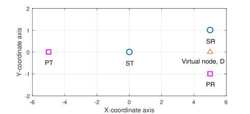
Refer to caption
Figure 2: Locations of PT, ST, PR and SR in X-Y coordinations.

V-A Performance Evaluation for the Perfect CSI case
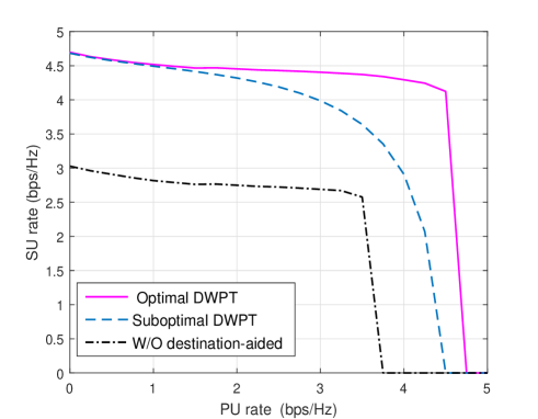
Refer to caption
Figure 3: SU-PU rate regions with PPโ€‹R=PSโ€‹R=30subscript๐‘ƒ๐‘ƒ๐‘…subscript๐‘ƒ๐‘†๐‘…30P_{PR}=P_{SR}=30 dBm.

At first, the achievable SU-PU rate regions are characterized in Fig. 3 for different schemes. A specific channel realization is randomly chosen as ๐ =[โˆ’0.2694โˆ’0.0123โ€‹i,โˆ’0.2221โˆ’0.0584โ€‹i,โˆ’0.1695+0.2270โ€‹i,โˆ’0.1823+0.1044โ€‹i]T๐ superscript0.26940.0123๐‘–0.22210.0584๐‘–0.16950.2270๐‘–0.18230.1044๐‘–๐‘‡\mathbf{g}=[-0.2694-0.0123i,-0.2221-0.0584i,-0.1695+0.2270i,-0.1823+0.1044i]^{T}, ๐กp=[โˆ’0.0762โˆ’0.1064โ€‹i,0.0060+0.2268โ€‹i,0.0962โˆ’0.3864โ€‹i,0.0037+0.0652โ€‹i]Tsubscript๐ก๐‘superscript0.07620.1064๐‘–0.00600.2268๐‘–0.09620.3864๐‘–0.00370.0652๐‘–๐‘‡\mathbf{h}_{p}=[-0.0762-0.1064i,0.0060+0.2268i,0.0962-0.3864i,0.0037+0.0652i]^{T} and ๐กs=[โˆ’0.0036+0.0617โ€‹i,โˆ’0.1718โˆ’0.0510โ€‹i,0.0218โˆ’0.1389โ€‹i,0.0480+0.2174โ€‹i]Tsubscript๐ก๐‘ superscript0.00360.0617๐‘–0.17180.0510๐‘–0.02180.1389๐‘–0.04800.2174๐‘–๐‘‡\mathbf{h}_{s}=[-0.0036+0.0617i,-0.1718-0.0510i,0.0218-0.1389i,0.0480+0.2174i]^{T}. It is observed that both optimal and suboptimal DWPT schemes achieve significantly larger rate region than the โ€˜w/o destination-aidedโ€™ scheme due to the destinationsโ€™ energy transfer. In addition, the optimal DWPT scheme always outperforms the suboptimal DWPT scheme. This is owing to the fact that the spatial degrees of freedom for the suboptimal scheme are slightly reduced by the decomposition of relay matrix ๐…๐…\mathbf{F} and the ZF design of receiver filter ๐Ÿrsubscript๐Ÿ๐‘Ÿ\mathbf{f}_{r}. Moreover, the SU rate of the low-complexity suboptimal DWPT scheme closely approaches to that of the optimal DWPT scheme when Rpmโ€‹iโ€‹nโ‰ค1.5superscriptsubscript๐‘…๐‘๐‘š๐‘–๐‘›1.5R_{p}^{min}\leq 1.5 bps/Hz. This is because that when the value of Rpmโ€‹iโ€‹nsuperscriptsubscript๐‘…๐‘๐‘š๐‘–๐‘›R_{p}^{min} is small, the allocated power for relay matrix ๐…๐…\mathbf{F} is extremely low such that the suboptimal design of ๐…๐…\mathbf{F} has little effect on the SU rate.

Refer to caption
Figure 4: Achievable SU rate versus transmission power at destinations (PR and SR) with Rpmโ€‹iโ€‹n=2.5superscriptsubscript๐‘…๐‘๐‘š๐‘–๐‘›2.5R_{p}^{min}=2.5 bps/Hz.

In Fig. 4, the impact of transmission power at PR and SR on the achievable SU rate is investigated with different energy conversion efficiencies ฮพ๐œ‰\xi. We assume that transmission power at PR and SR is equal to each other in our simulations. It is straightforward that the SU rate is improved as the transmission power at destinations increases. Note that, on one hand, the power aided by destinations enhances the amount of harvested energy at ST in the first phase from (3). On the other hand, based on (7) and (8), this power also brings additional interferences to PR and SR in the second phase. The continuous increasing SU rate with respect to transmission power at PR and SR indicates that, the interferences caused by destinationsโ€™ power transfer can be well suppressed and the desired signals with dominant power can benefit a lot from our proposed DWPT scheme. Besides, we can observe that the optimal DWPT scheme has obvious performance gain over the suboptimal scheme for different energy conversion efficiencies ฮพ๐œ‰\xi, while the gap between them gradually reduces when the transmission power at destinations increases. The reason is that when the transmission power at destinations is high, the system becomes interference-limited [24], and thus the suboptimal scheme with ZF-based receiver filter ๐Ÿrsubscript๐Ÿ๐‘Ÿ\mathbf{f}_{r} can cancel the strong interferences and approximately achieve the optimal performance.
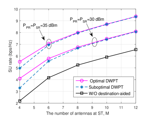
Refer to caption
Figure 5: Achievable SU rate versus the number of antennas at M with Rpmโ€‹iโ€‹n=2.5superscriptsubscript๐‘…๐‘๐‘š๐‘–๐‘›2.5R_{p}^{min}=2.5 bps/Hz.

Fig. 5 plots the achievable SU rates versus the number of antennas at ST for different schemes with Rpmโ€‹iโ€‹n=2.5superscriptsubscript๐‘…๐‘๐‘š๐‘–๐‘›2.5R_{p}^{min}=2.5 bps/Hz. For all schemes, as expected, more antennas employed by ST will result in better SU rate performance. In addition, it can be easily found that, the SU rate performance of the suboptimal scheme is gradually approaching to that of the optimal scheme with the increasing number of antennas at ST, especially when Mโ‰ฅ8๐‘€8M\geq 8. This is mainly because that, for the suboptimal scheme, the spatial degrees of freedom loss caused by the ZF-based receiver filter ๐Ÿrsubscript๐Ÿ๐‘Ÿ\mathbf{f}_{r} can be improved as M๐‘€M increases.

Refer to caption
Figure 6: Achievable SU rate versus dSโ€‹Tโˆ’D/dPโ€‹Tโˆ’Dsubscript๐‘‘๐‘†๐‘‡๐ทsubscript๐‘‘๐‘ƒ๐‘‡๐ทd_{ST-D}/d_{PT-D} with Rpmโ€‹iโ€‹n=2.5superscriptsubscript๐‘…๐‘๐‘š๐‘–๐‘›2.5R_{p}^{min}=2.5 bps/Hz.

To illustrate the impact of STโ€™s location on the SU rate in Fig. 6, we assume that ST can move along the X-coordinate axis from PT to D, a virtual node situated at (5, 0) as plotted in Fig. 2. dSโ€‹Tโˆ’Dsubscript๐‘‘๐‘†๐‘‡๐ทd_{ST-D} and dPโ€‹Tโˆ’Dsubscript๐‘‘๐‘ƒ๐‘‡๐ทd_{PT-D} respectively denote distances between ST and D, PT and D. From Fig. 6, it can be easily observed that our proposed DWPT scheme is greatly preferred when ST is close to PR and SR, since the amount of harvested energy at ST is effectively enhanced. Besides, it is of interest to find that, with the STโ€™s movement from PT to D (i.e., dSโ€‹Tโˆ’D/dPโ€‹Tโˆ’Dsubscript๐‘‘๐‘†๐‘‡๐ทsubscript๐‘‘๐‘ƒ๐‘‡๐ทd_{ST-D}/d_{PT-D} from 0.9 to 0.1), the achieved SU rates for all three schemes first decrease and then increase. And the worst point is moving to PT when transmission power of PR and SR is increasing. More curiously, the worst point of the โ€˜w/o destination-aidedโ€™ scheme occurs when dSโ€‹Tโˆ’D/dPโ€‹Tโˆ’Dsubscript๐‘‘๐‘†๐‘‡๐ทsubscript๐‘‘๐‘ƒ๐‘‡๐ทd_{ST-D}/d_{PT-D} ratio is 0.5 rather than 0.1. This is mainly due to the fact that, the harvested energy at ST is not enough to offset the severe path-loss between ST and PR/SR when ST is in the middle location.
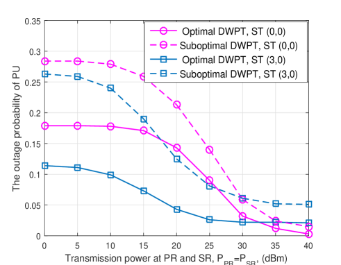
Refer to caption
Figure 7: The outage performance of PU versus transmission power at PR and SR with Rpmโ€‹iโ€‹n=2.5superscriptsubscript๐‘…๐‘๐‘š๐‘–๐‘›2.5R_{p}^{min}=2.5 bps/Hz.

In addition to the performance evaluation of achievable SU rate, we also investigate the outage performance of PU in Fig. 7. The outage will occur when the required rate demand of PU cannot be guaranteed. That is, the considered problem is infeasible. โ€˜ST (0, 0)โ€™ and โ€˜ST (3, 0)โ€™ in Fig. 7 respectively mean that ST is situated at (0, 0) and (3, 0) in Fig. 2. From Fig. 7, we can observe that the outage probability of PU is declining with the increase of transmission power at PR and SR. Combining Fig. 4 and Fig. 7, it is noted that when ST is located at (0, 0) and PPโ€‹R=PSโ€‹Rโ‰ฅ30subscript๐‘ƒ๐‘ƒ๐‘…subscript๐‘ƒ๐‘†๐‘…30P_{PR}=P_{SR}\geq 30 dBm, the growth trend of SU rate is very evident and the outage probability of PU is close to zero. This reveals that, not only SU but also PU can benefit from our proposed DWPT scheme. Furthermore, the proposed optimal DWPT scheme achieves better outage performance than the suboptimal scheme, and the gap between them reduces as transmission power at PR and SR increases. The reason behind this phenomenon is similar to Fig. 4. Besides, it can also be found that the outage performance of โ€˜ST (0, 0)โ€™ unexpectedly outperforms that of โ€˜ST (3, 0)โ€™ for both optimal and suboptimal DWPT schemes when PPโ€‹R=PSโ€‹Rโ‰ฅ30subscript๐‘ƒ๐‘ƒ๐‘…subscript๐‘ƒ๐‘†๐‘…30P_{PR}=P_{SR}\geq 30 dBm. This is mainly because that the interference at PR is stronger when ST is located at (3, 0). However, this slight worse outage performance of PU does not affect the improvement of SU rate when ST moves from (0, 0) to (3, 0) (i.e., dSโ€‹Tโˆ’D/dPโ€‹Tโˆ’Dsubscript๐‘‘๐‘†๐‘‡๐ทsubscript๐‘‘๐‘ƒ๐‘‡๐ทd_{ST-D}/d_{PT-D} from 0.5 to 0.2) according to Fig. 6.

V-B Performance Evaluation for the Imperfect CSI case
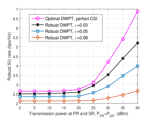
Refer to caption
Figure 8: Robust SU rate versus transmission power at PR and SR with Rpmโ€‹iโ€‹n=2.5superscriptsubscript๐‘…๐‘๐‘š๐‘–๐‘›2.5R_{p}^{min}=2.5 bps/Hz.

This subsection shows the performance evaluation for the imperfect CSI case. For simulation, we assume that the radii of channel uncertainty regions for ๐กpsubscript๐ก๐‘\mathbf{h}_{p} and ๐กssubscript๐ก๐‘ \mathbf{h}_{s} are equal to each other, i.e., ฮตp=ฮตs=ฮตsubscript๐œ€๐‘subscript๐œ€๐‘ ๐œ€\varepsilon_{p}=\varepsilon_{s}=\varepsilon. Other simulation parameters are the same as the perfect CSI case.

The achieved worst-case SU rates versus transmission power at PR and SR are characterized in Fig. 8 for different levels of channel uncertainty. The rate demand of PU is set as Rpmโ€‹iโ€‹n=2.5superscriptsubscript๐‘…๐‘๐‘š๐‘–๐‘›2.5R_{p}^{min}=2.5 bps/Hz. As can be seen, for both perfect and imperfect CSI cases, the larger value of transmission power at destinations, the better rate performance SU has. Furthermore, Observing from this figure, we can see that with the increase of channel uncertainty level, the achieved performance in terms of the worst-case SU rate is deteriorated.
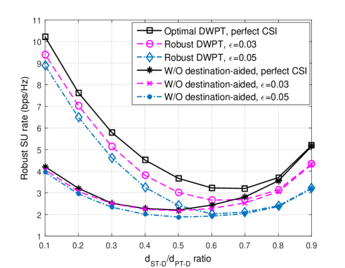
Refer to caption
Figure 9: Robust SU rate versus dSโ€‹Tโˆ’D/dPโ€‹Tโˆ’Dsubscript๐‘‘๐‘†๐‘‡๐ทsubscript๐‘‘๐‘ƒ๐‘‡๐ทd_{ST-D}/d_{PT-D} for different schemes with PPโ€‹R=PSโ€‹R=30subscript๐‘ƒ๐‘ƒ๐‘…subscript๐‘ƒ๐‘†๐‘…30P_{PR}=P_{SR}=30 dBm and Rpmโ€‹iโ€‹n=2.5superscriptsubscript๐‘…๐‘๐‘š๐‘–๐‘›2.5R_{p}^{min}=2.5 bps/Hz.

In Fig. 9, the impact of STโ€™s location on the worst-case robust SU rate is presented for different schemes. We assume that the rate demand of PU is Rpmโ€‹iโ€‹n=2.5superscriptsubscript๐‘…๐‘๐‘š๐‘–๐‘›2.5R_{p}^{min}=2.5 bps/Hz and the transmission power at each nodes is PPโ€‹R=PSโ€‹R=30subscript๐‘ƒ๐‘ƒ๐‘…subscript๐‘ƒ๐‘†๐‘…30P_{PR}=P_{SR}=30 dBm. Similar to the perfect CSI case, we can observe that our proposed robust DWPT scheme is also more preferred for all different channel uncertainty levels when ST is closer to destinations. Nevertheless, note that when ST is much closer to PT (i.e., dSโ€‹Tโˆ’D/dPโ€‹Tโˆ’Dโ†’0.9โ†’subscript๐‘‘๐‘†๐‘‡๐ทsubscript๐‘‘๐‘ƒ๐‘‡๐ท0.9d_{ST-D}/d_{PT-D}\to 0.9), the SU rates of the DWPT scheme for both perfect and imperfect CSI cases will fall to that of the โ€˜w/o destination-aidedโ€™ scheme. In this case, it is not necessary for destinations to assist power to ST.

VI Conclusion

This paper has proposed a DWPT scheme for a cognitive relay network, where the multiple-antenna energy-limited ST first harvests the energy sent by PT as well as PR and SR, and then relays the traffic from PT to PR and also serves SR. The relay process matrix, cognitive beamforming vector and power splitter have been jointly optimized to maximize the SU rate with the energy causality constraint and the constraint that the rate requirement of PU is met. Both the perfect and imperfect CSI scenarios have been investigated. For the former case, the global optimal and low-complexity suboptimal solutions have been presented. For the latter case, a worst-case robust algorithm has been proposed. It has been demonstrated in the simulation that our proposed DWPT scheme is greatly preferred when ST is close to PR and SR. Thus, the location-based relay selection scheme could be our future work.

Appendix A Proof of Proposition 1

Without loss of generality, similar to [25], ๐…๐…\mathbf{F} can be expressed as

๐…๐…\displaystyle{\mathbf{F}} =[๐•1โ€‹ย โ€‹๐•1โŠฅ]โ€‹[๐€โ€‹ย โ€‹๐๐‚โ€‹ย โ€‹๐ƒ]โ€‹[๐”2H๐”2โŠฅH]absentdelimited-[]subscript๐•1ย superscriptsubscript๐•1bottomdelimited-[]๐€ย ๐๐‚ย ๐ƒdelimited-[]superscriptsubscript๐”2๐ปsuperscriptsubscript๐”2bottom๐ป\displaystyle=\left[{{{\mathbf{V}}_{1}}{\text{ }}{\mathbf{V}}_{1}^{\bot}}\right]\left[\begin{gathered}{\mathbf{A}}{\text{ }}{\mathbf{B}}\hfill\\ {\mathbf{C}}{\text{ }}{\mathbf{D}}\hfill\\ \end{gathered}\right]\left[\begin{gathered}{\mathbf{U}}_{2}^{H}\hfill\\ {\mathbf{U}}_{2}^{\bot H}\hfill\\ \end{gathered}\right] (122)
=๐•1โ€‹๐€๐”2Hโ€‹ย +ย โ€‹๐•1โ€‹๐๐”2โŠฅH+๐•1โŠฅโ€‹๐‚๐”2H+๐•1โŠฅโ€‹๐ƒ๐”2โŠฅHabsentsubscript๐•1superscriptsubscript๐€๐”2๐ปย +ย subscript๐•1superscriptsubscript๐๐”2bottom๐ปsuperscriptsubscript๐•1bottomsuperscriptsubscript๐‚๐”2๐ปsuperscriptsubscript๐•1bottomsuperscriptsubscript๐ƒ๐”2bottom๐ป\displaystyle={{\mathbf{V}}_{1}}{\mathbf{AU}}_{2}^{H}{\text{ + }}{{\mathbf{V}}_{1}}{\mathbf{BU}}_{2}^{\bot H}+{\mathbf{V}}_{1}^{\bot}{\mathbf{CU}}_{2}^{H}+{\mathbf{V}}_{1}^{\bot}{\mathbf{DU}}_{2}^{\bot H}

where ๐•1โŠฅโˆˆโ„‚Mร—(Mโˆ’2)superscriptsubscript๐•1bottomsuperscriptโ„‚๐‘€๐‘€2{\mathbf{V}}_{1}^{\bot}\in{\mathbb{C}^{M\times(M-2)}}, ๐”2โŠฅโˆˆโ„‚Mร—(Mโˆ’3)superscriptsubscript๐”2bottomsuperscriptโ„‚๐‘€๐‘€3{\mathbf{U}}_{2}^{\bot}\in{\mathbb{C}^{M\times(M-3)}}, ๐€โˆˆโ„‚2ร—3๐€superscriptโ„‚23{\mathbf{A}}\in{\mathbb{C}^{2\times 3}}, ๐โˆˆโ„‚2ร—(Mโˆ’3)๐superscriptโ„‚2๐‘€3{\mathbf{B}}\in{\mathbb{C}^{2\times(M-3)}}, ๐‚โˆˆโ„‚(Mโˆ’2)ร—3๐‚superscriptโ„‚๐‘€23{\mathbf{C}}\in{\mathbb{C}^{(M-2)\times 3}} and ๐ƒโˆˆโ„‚(Mโˆ’2)ร—(Mโˆ’3)๐ƒsuperscriptโ„‚๐‘€2๐‘€3{\mathbf{D}}\in{\mathbb{C}^{(M-2)\times(M-3)}}. Obviously, ๐•1Hโ€‹๐•1โŠฅ=๐ŸŽsuperscriptsubscript๐•1๐ปsuperscriptsubscript๐•1bottom0{\mathbf{V}}_{1}^{H}{\mathbf{V}}_{1}^{\bot}={\mathbf{0}}, ๐”2โŠฅHโ€‹๐”2=๐ŸŽsuperscriptsubscript๐”2bottom๐ปsubscript๐”20{\mathbf{U}}_{2}^{\bot H}{\mathbf{U}}_{2}={\mathbf{0}}. Thus, we have

[๐กsH๐กpH]โ€‹๐•1โŠฅ=๐ŸŽ,๐”2โŠฅHโ€‹[๐กs,ย โ€‹๐กp,ย โ€‹๐ ]โ€‹ย =ย โ€‹๐ŸŽ.delimited-[]superscriptsubscript๐กs๐ปsuperscriptsubscript๐กp๐ปsuperscriptsubscript๐•1bottom0superscriptsubscript๐”2bottom๐ปsubscript๐กsย subscript๐กpย ๐ ย =ย 0\left[\begin{gathered}{\mathbf{h}}_{\text{s}}^{H}\hfill\\ {\mathbf{h}}_{\text{p}}^{H}\hfill\\ \end{gathered}\right]{\mathbf{V}}_{1}^{\bot}={\mathbf{0}},{\mathbf{U}}_{2}^{\bot H}\left[{{{\mathbf{h}}_{\text{s}}},{\text{ }}{{\mathbf{h}}_{\text{p}}},{\text{ }}{\mathbf{g}}}\right]{\text{ = }}{\mathbf{0}}. (123)

Substituting (116) into terms related to ๐…๐…\mathbf{F} in problem ๐’ซโ€‹1๐’ซ1\mathcal{P}1, we know that ๐๐\mathbf{B}, ๐‚๐‚\mathbf{C} and ๐ƒ๐ƒ\mathbf{D} do not affect |๐กsHโ€‹๐…๐ |2superscriptsuperscriptsubscript๐ก๐‘ ๐ป๐…๐ 2{\left|{{\mathbf{h}}_{s}^{H}{\mathbf{Fg}}}\right|^{2}}, |๐กsHโ€‹๐…๐กp|2superscriptsuperscriptsubscript๐ก๐‘ ๐ปsubscript๐…๐ก๐‘2{\left|{{\mathbf{h}}_{s}^{H}{\mathbf{F}}{{\mathbf{h}}_{p}}}\right|^{2}} and |๐กpHโ€‹๐…๐ |2superscriptsuperscriptsubscript๐ก๐‘๐ป๐…๐ 2{\left|{{\mathbf{h}}_{p}^{H}{\mathbf{Fg}}}\right|^{2}}. In addition, ๐‚๐‚\mathbf{C} and ๐ƒ๐ƒ\mathbf{D} have no impact on โ€–๐กsHโ€‹๐…โ€–22superscriptsubscriptnormsuperscriptsubscript๐ก๐‘ ๐ป๐…22{\left\|{{\mathbf{h}}_{s}^{H}{\mathbf{F}}}\right\|_{2}^{2}} and โ€–๐กpHโ€‹๐…โ€–22superscriptsubscriptnormsuperscriptsubscript๐ก๐‘๐ป๐…22{\left\|{{\mathbf{h}}_{p}^{H}{\mathbf{F}}}\right\|_{2}^{2}}, ๐๐\mathbf{B} and ๐ƒ๐ƒ\mathbf{D} have no effect on โ€–๐…๐ โ€–22superscriptsubscriptnorm๐…๐ 22\left\|{{\mathbf{Fg}}}\right\|_{2}^{2}, โ€–๐…๐กsโ€–22superscriptsubscriptnormsubscript๐…๐ก๐‘ 22\left\|{{\mathbf{F}}{{\mathbf{h}}_{s}}}\right\|_{2}^{2} and โ€–๐…๐กpโ€–22superscriptsubscriptnormsubscript๐…๐ก๐‘22\left\|{{\mathbf{F}}{{\mathbf{h}}_{p}}}\right\|_{2}^{2}. As a result, from (9) and (10), it is observed that ๐‚๐‚\mathbf{C} and ๐ƒ๐ƒ\mathbf{D} have no effect on SINRs of PR and SR. However, from (6), they increase the transmission power at ST. Hence, the optimal choice of ๐‚๐‚\mathbf{C} and ๐ƒ๐ƒ\mathbf{D} is ๐‚=๐ŸŽ๐‚0\mathbf{C}=\mathbf{0} and ๐ƒ=๐ŸŽ๐ƒ0\mathbf{D}=\mathbf{0}. Besides, both SINRs of PR and SR are increased if we set ๐=๐ŸŽ๐0\mathbf{B}=\mathbf{0}. Therefore, ๐…โ€‹ย =ย โ€‹๐•1โ€‹๐€๐”2H๐…ย =ย subscript๐•1superscriptsubscript๐€๐”2๐ป{\mathbf{F}}{\text{ = }}{{\mathbf{V}}_{1}}{\mathbf{AU}}_{2}^{H}.

Similarly, ๐ฐ๐ฐ\mathbf{w} can be expressed as

๐ฐโ€‹ย =ย โ€‹[๐•1,ย โ€‹๐•1โŠฅ]โ€‹[๐›๐œ]=๐•1โ€‹๐›+๐•1โŠฅโ€‹๐œ,๐ฐย =ย subscript๐•1ย superscriptsubscript๐•1bottomdelimited-[]๐›๐œsubscript๐•1๐›superscriptsubscript๐•1bottom๐œ{\mathbf{w}}{\text{ = }}\left[{{{\mathbf{V}}_{1}},{\text{ }}{\mathbf{V}}_{1}^{\bot}}\right]\left[\begin{gathered}{\mathbf{b}}\hfill\\ {\mathbf{c}}\hfill\\ \end{gathered}\right]={{\mathbf{V}}_{1}}{\mathbf{b}}+{\mathbf{V}}_{1}^{\bot}{\mathbf{c}}, (124)

where ๐›โˆˆโ„‚2ร—1๐›superscriptโ„‚21{\mathbf{b}}\in{\mathbb{C}^{2\times 1}} and ๐œโˆˆโ„‚(Mโˆ’2)ร—1๐œsuperscriptโ„‚๐‘€21{\mathbf{c}}\in{\mathbb{C}^{(M-2)\times 1}}. Note that ๐œ๐œ\mathbf{c} has no impact on โ€–๐กsHโ€‹๐ฐโ€–22superscriptsubscriptnormsuperscriptsubscript๐ก๐‘ ๐ป๐ฐ22{\left\|{{\mathbf{h}}_{s}^{H}{\mathbf{w}}}\right\|_{2}^{2}}, โ€–๐กpHโ€‹๐ฐโ€–22superscriptsubscriptnormsuperscriptsubscript๐ก๐‘๐ป๐ฐ22{\left\|{{\mathbf{h}}_{p}^{H}{\mathbf{w}}}\right\|_{2}^{2}}, and thus does not affect SINRs at PR and SR. But it increases the transmission power at ST. Hence, ๐œ=๐ŸŽ๐œ0\mathbf{c}=\mathbf{0} and ๐ฐ=๐•1โ€‹๐›๐ฐsubscript๐•1๐›\mathbf{w}=\mathbf{V}_{1}\mathbf{b}. This completes the proof. โˆŽ

References

  • [1] L.ย R. Varshney, โ€œTransporting information and energy simultaneously,โ€ in Proc. IEEE Information Theory (ISIT), July 2008, pp. 1612โ€“1616.
  • [2] R.ย Zhang and C.ย K. Ho, โ€œMIMO broadcasting for simultaneous wireless information and power transfer,โ€ IEEE Transactions on Wireless Communications, vol.ย 12, no.ย 5, pp. 1989โ€“2001, May 2013.
  • [3] Z.ย Zong, H.ย Feng, F.ย R. Yu, N.ย Zhao, T.ย Yang, and B.ย Hu, โ€œOptimal transceiver design for SWIPT in-user MIMO interference channels,โ€ IEEE Transactions on Wireless Communications, vol.ย 15, no.ย 1, pp. 430โ€“445, Jan. 2016.
  • [4] Y.ย Huang and B.ย Clerckx, โ€œJoint wireless information and power transfer for an autonomous multiple antenna relay system,โ€ IEEE Communications Letters, vol.ย 19, no.ย 7, pp. 1113โ€“1116, July 2015.
  • [5] M.ย Zhao, S.ย Feng, X.ย Wang, M.ย Zhang, Y.ย Liu, and H.ย Fu, โ€œJoint power splitting and secure beamforming design in the wireless-powered untrusted relay networks,โ€ in Proc. IEEE Global Communications Conference (GLOBECOM), Dec. 2015, pp. 1โ€“6.
  • [6] Y.ย Chen, Z.ย Wen, N.ย C. Beaulieu, S.ย Wang, and J.ย Sun, โ€œJoint source-relay design in a MIMO two-hop power-splitting-based relaying network,โ€ IEEE Communications Letters, vol.ย 19, no.ย 10, pp. 1746โ€“1749, Oct. 2015.
  • [7] A.ย A. Nasir, X.ย Zhou, S.ย Durrani, and R.ย A. Kennedy, โ€œThroughput and ergodic capacity of wireless energy harvesting based DF relaying network,โ€ in Proc. IEEE International Conference on Communications (ICC), June 2014, pp. 4066โ€“4071.
  • [8] G.ย Zheng, Z.ย Ho, E.ย A. Jorswieck, and B.ย Ottersten, โ€œInformation and energy cooperation in cognitive radio networks,โ€ IEEE Transactions on Signal Processing, vol.ย 62, no.ย 9, pp. 2290โ€“2303, May 2014.
  • [9] Y.ย Wang, W.ย Lin, R.ย Sun, and Y.ย Huo, โ€œOptimization of relay selection and ergodic capacity in cognitive radio sensor networks with wireless energy harvesting,โ€ Pervasive and Mobile Computing, vol.ย 22, pp. 33โ€“45, Sept. 2015.
  • [10] Y.ย Wang, R.ย Sun, and X.ย Wang, โ€œTransceiver design to maximize the weighted sum secrecy rate in full-duplex SWIPT systems,โ€ IEEE Signal Processing Letters, vol.ย 23, no.ย 6, pp. 883โ€“887, June 2016.
  • [11] Z.ย Wang, L.ย Li, H.ย Wang, and H.ย Tian, โ€œBeamforming design in relay based full-duplex MISO wireless powered communication networks,โ€ IEEE Communication Letters, early access, 2016.
  • [12] H.ย Ju and R.ย Zhang, โ€œThroughput maximization in wireless powered communication networks,โ€ IEEE Transactions on Wireless Communications, vol.ย 13, no.ย 1, pp. 418โ€“428, Jan. 2014.
  • [13] R.ย A. Horn and C.ย R. Johnson, Matrix analysis.ย ย ย Cambridge university press, 2012.
  • [14] L.ย Liu, R.ย Zhang, and K.-C. Chua, โ€œSecrecy wireless information and power transfer with MISO beamforming,โ€ IEEE Transactions on Signal Processing, vol.ย 62, no.ย 7, pp. 1850โ€“1863, Apr. 2014.
  • [15] M.ย Grant and S.ย Boyd, โ€œCVX: Matlab software for disciplined convex programming, version 1.22,โ€ 2012, online available: http://cvxr.com/cvx.
  • [16] Y.ย Huang and D.ย P. Palomar, โ€œRank-constrained separable semidefinite programming with applications to optimal beamforming,โ€ IEEE Transactions on Signal Processing, vol.ย 58, no.ย 2, pp. 664โ€“678, Feb. 2010.
  • [17] S.ย Boyd and L.ย Vandenberghe, Convex optimization.ย ย ย Cambridge University Press, 2004.
  • [18] G.ย Zheng, โ€œJoint beamforming optimization and power control for full-duplex MIMO two-way relay channel,โ€ IEEE Transactions on Signal Processing, vol.ย 63, no.ย 3, pp. 555โ€“566, Feb. 2015.
  • [19] D.ย Ponukumati, F.ย Gao, and C.ย Xing, โ€œRobust peer-to-peer relay beamforming: A probabilistic approach,โ€ IEEE Communications Letters, vol.ย 17, no.ย 2, pp. 305โ€“308, Feb. 2013.
  • [20] X.ย Yu and D.ย Park, โ€œOptimal beamforming design for information and power transmission in the presence of eavesdroppers,โ€ Wireless Personal Communications, vol.ย 83, no.ย 3, pp. 2193โ€“2209, Mar. 2015.
  • [21] Y.ย Sun, D.ย W.ย K. Ng, J.ย Zhu, and R.ย Schober, โ€œMulti-objective optimization for robust power efficient and secure full-duplex wireless communication systems,โ€ IEEE Transactions on Wireless Communications, vol.ย 15, no.ย 8, pp. 5511โ€“5526, Aug. 2016.
  • [22] Y.ย Wu and X.ย Chen, โ€œRobust beamforming and power splitting for secrecy wireless information and power transfer in cognitive relay networks,โ€ IEEE Communications Letters, vol.ย 20, no.ย 6, pp. 1152โ€“1155, June 2016.
  • [23] Z.-Q. Luo, W.-k. Ma, A.ย M.-C. So, Y.ย Ye, and S.ย Zhang, โ€œSemidefinite relaxation of quadratic optimization problems,โ€ IEEE Signal Processing Magazine, vol.ย 27, no.ย 3, pp. 20โ€“34, May 2010.
  • [24] D.ย Tse and P.ย Viswanath, Fundamentals of wireless communication.ย ย ย Cambridge university press, 2005.
  • [25] G.ย Zheng, S.ย Song, K.-K. Wong, and B.ย Ottersten, โ€œCooperative cognitive networks: optimal, distributed and low-complexity algorithms,โ€ IEEE Transactions on Signal Processing, vol.ย 61, no.ย 11, pp. 2778โ€“2790, June 2013.