Abstract

We examine various scenarios that involve a light ${\cal O}(1\ {\rm TeV})$ leptoquark state and select those which are compatible with the current experimental values for $\mathcal{B}(B_{s}\to\mu\mu)$, $\mathcal{B}(B\to K\mu\mu)_{\mathrm{large}-q^{2}}$, $R_{K}=\mathcal{B^{\prime}}(B\to K\mu\mu)/\mathcal{B^{\prime}}(B\to Kee)$, and which lead to predictions consistent with other experimental data. We show that two such scenarios are phenomenologically plausible, namely the one with a doublet of scalar leptoquarks of hypercharge $1/6$, and the one with a triplet of vector leptoquarks of hypercharge $2/3$. We also argue that a model with a singlet scalar leptoquark of hypercharge $1/3$ is not viable. Using the present experimental data as constraints, it is shown that the exclusive lepton flavor violating decays, $\mathcal{B}(B_{s}\to\mu\tau)$, $\mathcal{B}(B\to K\mu\tau)$ and $\mathcal{B}(B\to K^{\ast}\mu\tau)$, can be as large as $\mathcal{O}(10^{-5})$.

1 Introduction

The experimental searches of New Physics (NP) at the LHC are of great importance in our quest for solving the hierarchy and flavor problems. Rare decays and low-energy precision measurements play a crucial role in searching for the effects of physics beyond the Standard Model (BSM) because they are complementary to direct searches and even allow us to probe energy scales well above those that can be probed through them. Among the various types of rare decays, the lepton flavor violating (LFV) ones are particularly appealing because they are absent in the Standard Model (SM), and their detection would represent a clean signal of NP.

Theoretically, the LFV decays are predicted in various NP scenarios, such as in models with heavy sterile fermions [1], in models with a peculiar breaking of supersymmetry [2], in models involving an extra $Z^{\prime}$-boson [3], and in multiple scenarios founded on the paradigm of existence of one or more leptoquark (LQ) states [4]. Most of the current experimental efforts in searching for the effects of LFV are focused onto lepton decays, $\ell_{1}\to\ell_{2}\gamma$, $\ell_{1}\to 3\ell_{2}$ (with $\ell_{1,2}\in\{e,\mu,\tau\}$), and on the $\mu-e$ conversion in nuclei [5]. The experimental sensitivity to probe these decays is expected to be improved in the years to come by several orders of magnitude. The LFV decays of hadrons are complementary to the purely leptonic decays because they represent a convenient ground to test LQ models, and they also represent a different environment to test the result of the above-mentioned leptonic modes. For example, in the LQ models, which will be discussed in this paper, the rates of the LFV decays of hadrons are much larger than in radiative and three-body lepton decays.

In this paper we will focus on the exclusive LFV modes, $B_{s}\to\ell_{1}\ell_{2}$ and $B\to K^{(\ast)}\ell_{1}\ell_{2}$. At present, the most constraining experimental bound is $\mathcal{B}(B_{s}\to e^{\pm}\mu^{\mp})^{\mathrm{exp}}<1.1\times 10^{-8}$, which has been recently improved by an order of magnitude [6]. The only dedicated experimental searches with a $\tau$-lepton in the final state have been made by the BaBar Collaboration which reported the upper limits $\mathcal{B}(B^{+}\to K^{+}e^{\pm}\tau^{\mp})^{\mathrm{exp}}<3.0\times 10^{-5}$ and $\mathcal{B}(B^{+}\to K^{+}\mu^{\pm}\tau^{\mp})^{\mathrm{exp}}<4.8\times 10^{-5}$ [7]. The modes with one $\tau$-lepton in the final state are phenomenologically more appealing because the relevant couplings are less constrained by direct experimental limits and for that reason, in the following, we will focus on $B_{s}\to\mu\tau$ and $B\to K^{(\ast)}\mu\tau$.

One of the main motivations to study transitions based on $b\to s\ell_{1}\ell_{2}$ comes from the recent observation of lepton flavor universality (LFU) violation in 

$$R_{K}=\frac{\mathcal{B^{\prime}}(B^{+}\to K^{+}\mu\mu)}{\mathcal{B^{\prime}}(B^{+}\to K^{+}ee)}\equiv\left.\frac{\mathcal{B}(B^{+}\to K^{+}\mu\mu)}{\mathcal{B}(B^{+}\to K^{+}ee)}\right|_{q^{2}\in[1,6]\,\mathrm{GeV}^{2}},$$ (1)

where the squared dilepton mass is integrated in the bin $q^{2}\in[1,6]$ $\mathrm{GeV}^{2}$. LHCb found [8]

$$R_{K}^{\mathrm{exp}}=0.745^{+0.090}_{-0.074}(\mathrm{stat})\pm 0.036(\mathrm{syst}),$$ (2)

which is 2.4$\sigma$ lower than the SM prediction $R_{K}^{\mathrm{SM}}=1.00(1)$ [9, 10]. Since the hadronic uncertainties largely cancel in the ratio, if confirmed, this result would be an unambiguous manifestation of NP. Another experimental observation of LFU violation has been made in the processes mediated by the charged-current interaction, namely,

$$R_{D^{(\ast)}}=\dfrac{\mathcal{B}(B\to D^{(\ast)}\tau\nu)}{\mathcal{B}(B\to D^{(\ast)}\ell\nu)},\qquad\ell\in\{e,\mu\}\,,$$ (3)

which turned out to be $2\sigma$ (for $R_{D}$) and $3.4\sigma$ (for $R_{D^{\ast}}$) larger than predicted by the SM [11, 12, 13, 14, 15]. The possibility of connecting the observed LFU violation in neutral- and charged- current processes triggered many interesting theoretical works, mostly based on introducing various LQ states or new gauge bosons ($Z^{\prime}$ and $W^{\prime}$) [16, 19, 20, 21, 22]. Remarkably, in most of the proposed scenarios, LFV in meson decays is induced at observable rates [17, 18]. In a previous work, we computed the general expressions for the full angular distribution of $B_{s}\to\ell_{1}\ell_{2}$ and $B\to K^{(\ast)}\ell_{1}\ell_{2}$ decay modes, and explored a generic $Z^{\prime}$ model, as well as the possibility of a Higgs induced LFV [24]. In this paper we make a phenomenological analysis of the exclusive $b\to s\ell_{1}\ell_{2}$ decays in the LQ models which are compatible with the observed $R_{K}$.

The remainder of this paper is organized as follows. In Sec. 2 we remind the reader of the effective approach to $b\to s\ell_{1}\ell_{2}$ decays and briefly summarize the findings of Ref. [24]. In Sec. 3 we catalogue the plausible LQ models which are then scrutinized in Sec. 4 where we select the models compatible with the available $b\to s\mu\mu$ data. The models selected in that way, are then subjected to a phenomenological analysis in order to obtain upper bounds on the LFV $b\to s\ell_{1}\ell_{2}$ exclusive decay modes presented in Sec. 5. We summarize and conclude in Sec. 6. Most of the auxiliary formulas used in this paper are collected in the Appendices.

2 Effective Approach

The most general dimension-six effective Hamiltonian describing the LFV transitions $b\to s\ell_{1}^{-}\ell_{2}^{+}$, with $\ell_{1,2}\in\{e,\mu,\tau\}$) is defined by [25]

$$\begin{split}\mathcal{H}_{\mathrm{eff}}=-\frac{4G_{F}}{\sqrt{2}}V_{tb}V_{ts}^{*}&\Bigg{\{}\sum_{i=1}^{6}C_{i}(\mu)\mathcal{O}_{i}(\mu)+\sum_{i=7,8}\Big{[}C_{i}(\mu)\mathcal{O}_{i}(\mu)+\left(C_{i}(\mu)\right)^{\prime}\left(\mathcal{O}_{i}(\mu)\right)^{\prime}\Big{]}\\ &+\sum_{i=9,10,S,P}\Big{[}C^{\ell_{1}\ell_{2}}_{i}(\mu)\mathcal{O}^{\ell_{1}\ell_{2}}_{i}(\mu)+\left(C^{\ell_{1}\ell_{2}}_{i}(\mu)\right)^{\prime}\left(\mathcal{O}^{\ell_{1}\ell_{2}}_{i}(\mu)\right)^{\prime}\Big{]}\Bigg{\}}+\mathrm{h.c.},\end{split}$$ (4)

where $C_{i}(\mu)$ and $C_{i}^{\ell_{1}\ell_{2}}(\mu)$ are the Wilson coefficients, while the effective operators relevant to our study are defined by

$$\begin{split}\mathcal{O}_{9}^{\ell_{1}\ell_{2}}&=\frac{e^{2}}{(4\pi)^{2}}(\bar{s}\gamma_{\mu}P_{L}b)(\bar{\ell}_{1}\gamma^{\mu}\ell_{2}),\qquad\qquad\hskip 11.38092pt\mathcal{O}_{S}^{\ell_{1}\ell_{2}}=\frac{e^{2}}{(4\pi)^{2}}(\bar{s}P_{R}b)(\bar{\ell}_{1}\ell_{2}),\\ \mathcal{O}_{10}^{\ell_{1}\ell_{2}}&=\frac{e^{2}}{(4\pi)^{2}}(\bar{s}\gamma_{\mu}P_{L}b)(\bar{\ell}_{1}\gamma^{\mu}\gamma^{5}\ell_{2}),\qquad\qquad\mathcal{O}_{P}^{\ell_{1}\ell_{2}}=\frac{e^{2}}{(4\pi)^{2}}(\bar{s}P_{R}b)(\bar{\ell}_{1}\gamma^{5}\ell_{2}),\end{split}$$ (5)

in addition to the electromagnetic penguin operator, $\mathcal{O}_{7}=e/(4\pi)^{2}m_{b}(\bar{s}\sigma_{\mu\nu}P_{R}b)F^{\mu\nu}$. The chirality flipped operators $\mathcal{O}_{i}^{\prime}$ are obtained from $\mathcal{O}_{i}$ by the replacement $P_{L}\leftrightarrow P_{R}$. Using the above Hamiltonian, one can easily compute the amplitudes for $B_{s}\to\ell_{1}^{-}\ell^{+}_{2}$ and $B\to K^{(\ast)}\ell_{1}^{-}\ell^{+}_{2}$ decays, and derive the expressions for the corresponding decay rates [24, 26], also summarized in Appendix A.3 of the present paper. In the SM, the LFV Wilson coefficients, $C_{i}^{\ell_{1}\ell_{2}}$, are zero due to lepton flavor conservation. The inclusion of neutrino masses can induce LFV at the loop-level, but with negligible rates due to the smallness of the neutrino masses. In the following we shall assume that the only source of LFV is NP and hence in order to compute the Wilson coefficients for $b\to s\ell_{1}\ell_{2}$ ($\ell_{1}\neq\ell_{2}$) we need to specify the NP model.

To simplify our notation, in what follows, we will denote $C_{i}\equiv C_{i}^{\ell_{1}\ell_{2}}$ ($\ell_{1}\neq\ell_{2}$) when confusion can be avoided. Notice, however, that:

• in general, for $\ell_{1}\neq\ell_{2}$, $C_{i}^{\ell_{1}\ell_{2}}\neq C_{i}^{\ell_{2}\ell_{1}}$, which is particularly the case in the LQ models in which LFV occurs through tree-level diagrams;

• in some situations, even if $C_{i}^{\ell_{1}\ell_{2}}=C_{i}^{\ell_{2}\ell_{1}}$, $\forall i$, one can still generate an asymmetry between LFV modes with different lepton charges, e.g. $\mathcal{B}(B_{s}\to\mu^{-}\tau^{+})\neq\mathcal{B}(B_{s}\to\mu^{+}\tau^{-})$, cf. expressions in Appendix A.3.

Before discussing the issue of lepton charge asymmetry one must first observe LFV, that is why we will here combine the two charged modes, namely, $\mathcal{B}(B_{s}\to\ell_{1}\ell_{2})\equiv\mathcal{B}(B_{s}\to\ell_{1}^{-}\ell_{2}^{+})+\mathcal{B}(B_{s}\to\ell_{1}^{+}\ell_{2}^{-})$, and $\mathcal{B}(B\to K^{(\ast)}\ell_{1}\ell_{2})\equiv\mathcal{B}(B\to K^{(\ast)}\ell_{1}^{-}\ell_{2}^{+})+\mathcal{B}(B\to K^{(\ast)}\ell_{1}^{+}\ell_{2}^{-})$.

We should also emphasize that the LFV channels we consider respect a hierarchy which depends on the adopted NP scenario. If the LFV is generated only by the (pseudo-)scalar operators, the lifted helicity suppression implies

$$C_{S,P}^{(\prime)}\neq 0,C_{9,10}^{(\prime)}=0:\hskip 34.14322pt\mathcal{B}(B_{s}\to\ell_{1}\ell_{2})>\mathcal{B}(B\to K\ell_{1}\ell_{2})>\mathcal{B}(B\to K^{\ast}\ell_{1}\ell_{2}),$$ (6)

whereas the inverted hiearchy is obtained if the nonzero Wilson coefficients are those corresponding to the (axial-)vector operators ($C_{S,P}^{(\prime)}=0$, $C_{9,10}^{(\prime)}\neq 0$) [24].

3 $C_{i}^{\ell_{1}\ell_{2}}(\mu)$ in Leptoquark Models

Leptoquarks are colored states that can mediate interactions between quarks and leptons. Such particles can appear in Grand Unified Theories [27] and in models with composite Higgs states [28], as recently reviewed in [4]. In general, a LQ can be a scalar or a vector field which in turn can come as an $SU(2)_{L}$-singlet, -doublet or -triplet [29]. In the following we assume that the SM is extended by only one of the LQ states and list the models which can be used to describe the $b\to s\ell_{1}\ell_{2}$ processes. We adopt the notation of Ref. [30] and specify the LQ states by their quantum numbers with respect to the SM gauge group, $(SU(3)_{c},SU(2)_{L})_{Y}$, where the electric charge, $Q=Y+T_{3}$, is the sum of hypercharge ($Y$) and the third weak isospin component ($T_{3}$). Throughout this paper the flavor indices of LQ couplings will refer to the mass eigenstates of down-type quarks and charged leptons, unless stated otherwise. In other words, the left-handed doublets are defined as $Q_{i}=[(V^{\dagger}u_{L})_{i}\;d_{Li}]^{T}$ and $L_{i}=[(U\nu_{L})_{i}\;\ell_{Li}]^{T}$, where $V$ and $U$ are the Cabibbo-Kobayashi-Maskawa (CKM) and the Pontecorvo-Maki-Nakagawa-Sakata (PMNS) matrices, respectively, $u_{L}$, $d_{L}$, $\ell_{L}$ are the fermion mass eigenstates, whereas $\nu_{L}$ stand for the massless neutrino flavor eigenstates. Since the tiny neutrino masses play no role for the purpose of this paper, we may choose the PMNS matrix to be the unity matrix, $U=\mathbb{1}$. Right-handed field indices will always refer to the mass eigenbasis.

3.1 Scalar Leptoquarks

We first consider three scalar LQ scenarios. Two of them can modify the $b\to s\mu\tau$ decay at tree-level without spoiling the proton stability. A third scenario, which might destabilise the proton and will also be discussed below, generates a contribution to $b\to s\mu\tau$ only at the loop-level.

3.1.1 ${\Delta}^{(1/6)}\equiv(3,2)_{1/6}$

This model has already been used to provide a viable explanation of $R_{K}^{\mathrm{exp}}$ in Ref. [19]. The Yukawa Lagrangian reads,

$$\begin{split}\mathcal{L}_{\Delta^{(1/6)}}&=(g_{L})_{ij}\bar{d}_{Ri}{\widetilde{\bm{\Delta}}}^{(1/6)\dagger}L_{j}+\mathrm{h.c.},\\ &=\left(g_{L}\right)_{ij}\bar{d}_{i}P_{L}\nu_{j}\,\Delta^{(-1/3)}-(g_{L})_{ij}\bar{d}_{i}P_{L}\ell_{j}\,\Delta^{(2/3)}+\mathrm{h.c.},\end{split}$$ (7)

where $\widetilde{\bm{\Delta}}\equiv i\tau_{2}{\bm{\Delta}}^{\ast}$ is the conjugated $SU(2)_{L}$ doublet, $g_{L}$ is a generic matrix of couplings. In the second line we explicitly write the terms with $\Delta^{(-1/3)}$ and $\Delta^{(2/3)}$ where the superscripts refer to the electric charge of the $Y=1/6$ LQ states. The masses of these two states can in principle be different, but for simplicity we will assume them to be equal, $m_{\Delta^{(2/3)}}=m_{\Delta^{(-1/3)}}\equiv m_{\Delta}$. . After integrating out the heavy fields, this model gives rise to the chirality flipped operators in the $b\to s\ell_{1}^{-}\ell_{2}^{+}$ effective Hamiltonian (4), and the corresponding Wilson coefficients are given by

$$\left(C_{9}^{\ell_{1}\ell_{2}}\right)^{\prime}=-\left(C_{10}^{\ell_{1}\ell_{2}}\right)^{\prime}=-\frac{\pi v^{2}}{2V_{tb}V_{ts}^{\ast}\alpha_{\mathrm{em}}}\frac{(g_{L})_{s\ell_{1}}(g_{L})_{b\ell_{2}}^{\ast}}{m_{\Delta}^{2}},$$ (8)

where $v=246$ GeV is the well known electroweak vacuum expectation value, $v^{2}=1/(\sqrt{2}G_{F})$.

3.1.2 ${\Delta}^{(7/6)}\equiv(3,2)_{7/6}$

The relevant Lagrangian for this model reads,

$$\begin{split}\mathcal{L}_{\Delta^{(7/6)}}&=(g_{R})_{ij}\bar{Q}_{i}{\bm{\Delta}}^{(7/6)}\ell_{Rj}+\mathrm{h.c.},\\ &=(Vg_{R})_{ij}\bar{u}_{i}P_{R}\ell_{j}\,\Delta^{(5/3)}+(g_{R})_{ij}\bar{d}_{i}P_{R}\ell_{j}\,\Delta^{(2/3)}+\mathrm{h.c.},\end{split}$$ (9)

where $g_{R}$ denotes the Yukawa coupling matrix, while again the superscript in $\Delta^{(5/3)}$ and $\Delta^{(2/3)}$ refers to the electric charge of the two mass degenerate LQ states. After integrating out the heavy fields, the only non-zero Wilson coefficients relevant to $b\to s\ell_{1}^{-}\ell_{2}^{+}$ are,

$$C_{9}^{\ell_{1}\ell_{2}}=C_{10}^{\ell_{1}\ell_{2}}=-\frac{\pi v^{2}}{2V_{tb}V_{ts}^{\ast}\alpha_{\mathrm{em}}}\frac{(g_{R})_{s\ell_{1}}(g_{R})_{b\ell_{2}}^{\ast}}{m_{\Delta}^{2}},$$ (10)

corresponding to the chirality non-flipped operators in Eq. (4).

3.1.3 $\Delta^{(1/3)}\equiv(3,1)_{-1/3}$

Being an electroweak singlet, this scalar LQ model is the simplest one. Its Lagrangian is given by,

$$\begin{split}\mathcal{L}_{\Delta^{(1/3)}}&=(g_{L})_{ij}\overline{Q_{i}^{C}}i\tau_{2}L_{j}\Delta^{(1/3)\ast}+(g_{R})_{ij}\overline{u_{Ri}^{C}}\ell_{Rj}{\Delta^{(1/3)\ast}}+\mathrm{h.c.}\\ &={\Delta^{(1/3)\ast}}\Big{[}(V^{\ast}g_{L})_{ij}\overline{u_{i}^{C}}P_{L}\ell_{j}-(g_{L})_{ij}\overline{d_{i}^{C}}P_{L}\nu_{j}+(g_{R})_{ij}\overline{u_{i}^{C}}P_{R}\ell_{j}\Big{]}+\mathrm{h.c.},\end{split}$$ (11)

where the superscript $C$ stands for the charge conjugation.  In addition to terms shown in (11) one could also write terms involving diquarks. To avoid conflict with the proton decay bounds those couplings must be negligible, so we set them here to zero.

The Wilson coefficients contributing to $b\to s\ell_{1}^{-}\ell_{2}^{+}$ are generated at loop level and, to one-loop order, they are given by [21, 33]:

$$C_{9}^{\ell_{1}\ell_{2}}-C_{10}^{\ell_{1}\ell_{2}} =\frac{m_{t}^{2}}{8\pi\alpha_{\mathrm{em}}m_{\Delta}^{2}}(V^{\ast}g_{L})_{t\ell_{1}}^{\ast}(V^{\ast}g_{L})_{t\ell_{2}}-\frac{1}{64\pi\alpha_{\mathrm{em}}}\frac{v^{2}}{m_{\Delta}^{2}}\frac{(g_{L}\cdot g_{L}^{\dagger})_{bs}}{V_{tb}V_{ts}^{\ast}}(g_{L}^{\dagger}\cdot g_{L})_{\ell_{1}\ell_{2}},$$ (12)

$$C_{9}^{\ell_{1}\ell_{2}}+C_{10}^{\ell_{1}\ell_{2}} =\frac{m_{t}^{2}}{16\pi\alpha_{\mathrm{em}}m_{\Delta}^{2}}(g_{R})_{t\ell_{1}}^{\ast}(g_{R})_{t\ell_{2}}\Bigg{[}\log\frac{m_{\Delta}^{2}}{m_{t}^{2}}-f(x_{t})\Bigg{]}-\frac{1}{64\pi\alpha_{\mathrm{em}}}\frac{v^{2}}{m_{\Delta}^{2}}\frac{(g_{L}\cdot g_{L}^{\dagger})_{bs}}{V_{tb}V_{ts}^{\ast}}(g_{R}^{\dagger}\cdot g_{R})_{\ell_{1}\ell_{2}},$$ (13)

where $f(x_{t})=1+\dfrac{3}{x_{t}-1}\left(\dfrac{\log x_{t}}{x_{t}-1}-1\right)$, and $x_{t}=m_{t}^{2}/m_{W}^{2}$.

3.2 Vector Leptoquarks

Vector LQs naturally appear in Grand Unified Theories as gauge bosons of the unified gauge group or in composite Higgs scenarios. Here we shall focus on relatively light vector LQs that can contribute to LFV $b\to s\ell_{1}\ell_{2}$ transitions. There are three vector LQ states that could participate in $d_{i}\to d_{j}\ell_{1}\ell_{2}$ processes via dimension-$4$ tree-level couplings to the SM fermions. These states, $\bm{U}_{3}$, $\bm{V}_{2}$, and $U_{1}$, are respectively a weak triplet, doublet, and singlet under the $SU(2)_{L}$. Here we do not consider the weak doublet vector $\bm{V}_{2}$, because its nonzero couplings might jeopardize the proton stability [30].

3.2.1 $U_{1}\equiv(3,1)_{2/3}$

Being a $SU(2)_{L}$ singlet $U_{1}$ can couple to both the left-handed and right-handed fermions, namely,

$$\begin{split}\mathcal{L}_{U_{1}}&=x^{LL}_{ij}\bar{Q}_{i}\gamma_{\mu}U_{1}^{\mu}L_{j}+x^{RR}_{ij}\bar{d}_{Ri}\gamma_{\mu}U_{1}^{\mu}\ell_{Rj}+\mathrm{h.c.}\\ &=U_{1\mu}\Big{[}(Vx^{LL})_{ij}\bar{u}_{i}\gamma^{\mu}P_{L}\nu_{j}+x^{LL}_{ij}d_{i}\gamma^{\mu}P_{L}\ell_{j}+x^{RR}_{ij}\bar{d}_{i}\gamma^{\mu}P_{R}\ell_{j}\Big{]}+\mathrm{h.c.},\end{split}$$ (14)

where $x^{LL}_{ij}$ and $x^{RR}_{ij}$ are the matrices of Yukawa couplings. The non-chiral nature of $U_{1}$ couplings to fermions induces both vector and scalar Wilson coefficients:

$$C_{9}^{\ell_{1}\ell_{2}} =-C_{10}^{\ell_{1}\ell_{2}} =-\frac{\pi v^{2}}{V_{tb}V_{ts}^{\ast}\alpha_{\mathrm{em}}m_{U}^{2}}x^{LL}_{s\ell_{2}}x_{b\ell_{1}}^{LL\ast},$$

$$\left(C_{9}^{\ell_{1}\ell_{2}}\right)^{\prime} =\left(C_{10}^{\ell_{1}\ell_{2}}\right)^{\prime} =-\frac{\pi v^{2}}{V_{tb}V_{ts}^{\ast}\alpha_{\mathrm{em}}m_{U}^{2}}x^{RR}_{s\ell_{2}}x_{b\ell_{1}}^{RR\ast},$$ (15)

$$C_{S}^{\ell_{1}\ell_{2}} =-C_{P}^{\ell_{1}\ell_{2}} =\frac{2\pi v^{2}}{V_{tb}V_{ts}^{\ast}\alpha_{\mathrm{em}}m_{U}^{2}}x^{LL}_{s\ell_{2}}x_{b\ell_{1}}^{RR\ast},$$

$$\left(C_{S}^{\ell_{1}\ell_{2}}\right)^{\prime} =\left(C_{P}^{\ell_{1}\ell_{2}}\right)^{\prime} =\frac{2\pi v^{2}}{V_{tb}V_{ts}^{\ast}\alpha_{\mathrm{em}}m_{U}^{2}}x^{RR}_{s\ell_{2}}x_{b\ell_{1}}^{LL\ast},$$

where $m_{U}$ is the LQ mass. Obviously this model provides a rich ground for phenomenology because it gives rise to both the chirality flipped and non-flipped operators.

3.2.2 ${U_{3}}\equiv(3,3)_{2/3}$

The only possible dimension-$4$ gauge invariant interaction between $\bm{U}_{3}$, a weak triplet of LQ states, and fermions reads

$$\begin{split}\mathcal{L}_{U_{3}}&=x^{LL}_{ij}\bar{Q}_{i}\gamma_{\mu}\bm{\tau}\cdot\bm{U}_{3}^{\mu}L_{j}+\mathrm{h.c.}\\ &=U^{(2/3)}_{3\mu}\,\Big{[}(Vx^{LL})_{ij}\,\bar{u}_{i}\gamma^{\mu}P_{L}\nu_{j}-x^{LL}_{ij}\,\bar{d}_{i}\gamma^{\mu}P_{L}\ell_{j}\Big{]}\\ &\quad+U^{(5/3)}_{3\mu}\,(\sqrt{2}Vx^{LL})_{ij}\,\bar{u}_{i}\gamma^{\mu}P_{L}\ell_{j}\\ &\quad+U^{(-1/3)}_{3\mu}\,(\sqrt{2}x^{LL})_{ij}\,\bar{d}_{i}\gamma^{\mu}P_{L}\nu_{j}+\mathrm{h.c.}\end{split}$$ (16)

where by $x^{LL}_{ij}$ we denote the couplings to the SM quarks and lepton doublets. The absence of diquark couplings guarantees that this LQ state is both baryon and lepton number conserving. The Wilson coefficients for the $b\to s\ell_{1}\ell_{2}$ Hamiltonian are in the case of $\bm{U}_{3}$ obtained by keeping nonzero only the $x^{LL}$ couplings in Eq. (3.2.1). For completeness we write them explicitly,

$$C_{9}^{\ell_{1}\ell_{2}} =-C_{10}^{\ell_{1}\ell_{2}}=-\frac{\pi v^{2}}{V_{tb}V_{ts}^{\ast}\alpha_{\mathrm{em}}m_{U}^{2}}x^{LL}_{s\ell_{2}}x_{b\ell_{1}}^{LL\ast},$$ (17)

where we assume the degeneracy among the charge eigenstates of the triplet, $m_{U}\equiv m_{U^{(-1/3)}}=m_{U^{(2/3)}}=m_{U^{(5/3)}}$.

4 Confronting LQ models with data

4.1 Which leptoquark model?

In this Section, from the list of models spelled out in Sec. 3, we select those that are consistent with the experimental data for the exclusive $b\to s\mu\mu$ processes. To that end we require the consistency with the measured $\mathcal{B}(B_{s}\to\mu^{+}\mu^{-})^{\mathrm{exp}}=(2.8^{+0.7}_{-0.6})\times 10^{-9}$ [34],  and $\mathcal{B}(B\to K\mu^{+}\mu^{-})_{\text{high}-q^{2}}^{\mathrm{exp}}=(8.5\pm 0.3\pm 0.4)\times 10^{-8}$ [36], since in that region of $q^{2}\in[15,22]\,{\rm GeV}^{2}$ the hadronic uncertainties are well controlled by means of numerical simulations of QCD on the lattice [37]. Furthermore, by choosing $q^{2}\in[15,22]\ {\rm GeV}^{2}$ we also avoid the narrow charmonium resonances so that we can rely on the quark-hadron duality [38]. This is also the reason why we use only $\mathcal{B}(B_{s}\to\mu^{+}\mu^{-})$ and $\mathcal{B}(B\to K\mu^{+}\mu^{-})_{{\rm high}-q^{2}}$ to derive the constraints on possible NP contributions: (a) They involve the decay constant $f_{B_{s}}$ and a few form factors at large $q^{2}$’s, the quantities which have been accurately computed by means of lattice QCD; (b) These quantities are not plagued by uncertainties related to the $c\bar{c}$-resonances. Theoretical description of $B\to K^{\ast}\mu^{+}\mu^{-}$ decay entails more hadronic form factors and more assumptions are needed when confronting theory with experiment. Similarly, a recently observed discrepancy between theory and experiment regarding $\mathcal{B}(B_{s}\to\phi\mu^{+}\mu^{-})$ [39] relies on the assumption of validity of the light cone QCD sum rule estimates of the hadronic form factors at low and intermediate $q^{2}$’s for which the systematic uncertainties are hard to assess. Furthermore, for the purpose of our study, two measured quantities are sufficient to bound the NP couplings and we choose those which require the least number of assumptions, i.e. $\mathcal{B}(B_{s}\to\mu^{+}\mu^{-})$ and $\mathcal{B}(B\to K\mu^{+}\mu^{-})_{{\rm high}-q^{2}}$. Notice, however, that our results are compatible, at a $(2\div 3)\sigma$ level, with the global fit analyses made in Ref. [40].

• The ${\bm{\Delta}}^{(1/6)}$-model was studied in Ref. [19] where it has been shown that the required consistency with the measured $\mathcal{B}(B_{s}\to\mu^{+}\mu^{-})^{\mathrm{exp}}$ and $\mathcal{B}(B\to K\mu^{+}\mu^{-})_{\text{high}-q^{2}}^{\mathrm{exp}}$ results in the $R_{K}$ values fully compatible with experiment.  In this scenario $(C_{9})^{\prime}=-(C_{{10}})^{\prime}$, and from the combined fit of $\mathcal{B}(B_{s}\to\mu^{+}\mu^{-})$ and $\mathcal{B}(B\to K\mu^{+}\mu^{-})_{\text{high}-q^{2}}$ we obtain to $2\sigma$ accuracy,

  $$(C_{9}^{\mu\mu})^{\prime}\in(-0.41,-0.08)_{\scriptscriptstyle\rm HPQCD},\ (-0.48,-0.17)_{\scriptscriptstyle\rm MILC},$$ (18)

  where the results in the first and second interval are obtained by using the hadronic form factors computed in lattice QCD in Ref. [42] and Ref. [43], respectively. Notice that the first interval coincides with what is obtained in Ref. [19]. In what follows we will choose

  $$(C_{9}^{\mu\mu})^{\prime}\in(-0.48,-0.08)\,,$$ (19)

  which covers both of the above intervals.

• For the ${\bm{\Delta}}^{(7/6)}$-model, the NP Wilson coefficients satisfy the relation $C_{9}=C_{10}$. To scrutinize this scenario, we perform a fit of $C_{9,10}$ assuming them to be real and by applying the strategy described above. The allowed regions at $1\sigma$ and $2\sigma$ are shown in Fig. 1 where we also draw the lines corresponding to $C_{9}=\pm C_{10}$. Clearly, the line $C_{9}=C_{10}$ does not touch the region allowed by $\mathcal{B}(B_{s}\to\mu^{+}\mu^{-})^{\mathrm{exp}}$ and $\mathcal{B}(B\to K\mu^{+}\mu^{-})_{{\rm high}-q^{2}}^{\mathrm{exp}}$ to $2\sigma$. For that reason we discard the scenario ${\bm{\Delta}}^{(7/6)}$ from further discussion. 

  

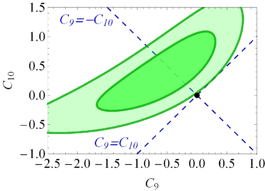
  Figure 1: Regions in the plane $(C_{9}^{\mu\mu},C_{10}^{\mu\mu})$ that are in agreement with the experimental values of ${\mathcal{B}}(B_{s}\to\mu\mu)$ and ${\mathcal{B}}(B^{+}\to K^{+}\mu\mu)_{{\rm large}\ q^{2}}$ at $1\sigma$ (dark green) and $2\sigma$ (light green) accuracy. The black point represents the SM prediction. The dashed lines correspond to the scenarios $C_{9}^{\mu\mu}=-C_{10}^{\mu\mu}$ and $C_{9}^{\mu\mu}=C_{10}^{\mu\mu}$.

• The $\Delta^{(1/3)}$-model generates both $C_{9}-C_{10}$ and $C_{9}+C_{10}$. In other words, this model is compatible with exclusive $b\to s\mu\mu$ data only if the combination with the plus sign is suppressed. One can achieve that by taking $(g_{R})_{ij}\approx 0$ in Eq. (13), or by fine-tuning the terms in the same equation to get $C_{9}+C_{10}\approx 0$. We will discuss more extensively this model in the next subsection.

• The ${\bm{U}_{3}}$-model was already studied in Ref. [20] where it has been shown that it can provide a simultaneous explanation of $R_{K}^{\mathrm{exp}}$ and $R_{D^{(\ast)}}^{\mathrm{exp}}$. In this scenario $C_{9}=-C_{10}$, which is in agreement with the measured $\mathcal{B}(B_{s}\to\mu^{+}\mu^{-})^{\mathrm{exp}}$ and $\mathcal{B}(B\to K\mu^{+}\mu^{-})_{{\rm high}-q^{2}}^{\mathrm{exp}}$, as shown in Fig. 1. To $2\sigma$ accuracy we find

  $$C_{9}^{\mu\mu}\in(-0.71,-0.04)_{\scriptscriptstyle\rm HPQCD},\ (-0.76,-0.11)_{\scriptscriptstyle\rm MILC}.$$ (20)

  As before, we will use

  $$C_{9}^{\mu\mu}\in(-0.76,-0.04)$$ (21)

  to cover the results obtained by using both sets of lattice QCD form factors.

• A similar discussion applies to the $U_{1}$ LQ in the limit of $|x^{RR}_{ij}|\ll|x^{LL}_{ij}|$ in Eq. (3.2.1). We should emphasize, however, that this model is not phenomenologically sound because the couplings to $\tau$’s are very poorly constrained by data. Since one cannot compute the loop corrections with vector LQs without specifying the ultraviolet (UV) completion or providing an explicit UV cut-off, no constraints from $B_{s}-\bar{B}_{s}$ and $\tau\to\mu\gamma$ can be used. While in the $\bm{U}_{3}$-model one can obtain a constraint by requiring the consistency between the tree-level process $\mathcal{B}(B\to K\nu\nu)$ and the upper experimental bound, in the $U_{1}$-model the latter process is induced only at the loop-level and the experimental result is not constraining anymore. For this reason we prefer to discard the $U_{1}$-model and focus only on the scenario with $\bm{U}_{3}$, as far as vector LQs are concerned.

In summary, of all the LQ models discussed in Sec. 3, we were able to discard in this section the scalar ${\bm{\Delta}}^{(7/6)}$ and the vector $U_{1}$. The remaining models can now be used to explore what are the allowed $b\to s\mu\tau$ LFV decay rates. Before passing into that part, we revisit the $\Delta^{(1/3)}$-model.

4.2 On (in)viability of $\Delta^{(1/3)}\equiv(3,1)_{-1/3}$

The interest in the $\Delta^{(1/3)}$-model has been recently revived after the authors of Ref. [21] claimed that it can simultaneously accommodate the observed LFU violation in $R_{K}$ and $R_{D^{(\ast)}}$. In this section we revisit that claim and find that $R_{K}$ actually cannot be made significantly smaller than one, without running into serious difficulties with other measured quantities.

As we already mentioned above, the effective coefficients $C_{9}^{\ell_{1}\ell_{2}}\pm C_{10}^{\ell_{1}\ell_{2}}$ are loop induced and the results are given in Eqs. (12)-(13). To suppress the combination with the plus sign, which is disfavored by the current $b\to s\mu\mu$ exclusive data, we set $g_{R}=0$ in Eq. (11).  The left-handed couplings are assumed to have the following flavor structure

$$g_{L}=\begin{pmatrix}0&0&0\\ 0&(g_{L})_{s\mu}&(g_{L})_{s\tau}\\ 0&(g_{L})_{b\mu}&(g_{L})_{b\tau}\end{pmatrix},\qquad Vg_{L}=\begin{pmatrix}0&V_{us}(g_{L})_{s\mu}+V_{ub}(g_{L})_{b\mu}&V_{us}(g_{L})_{s\tau}+V_{ub}(g_{L})_{b\tau}\\ 0&V_{cs}(g_{L})_{s\mu}+V_{cb}(g_{L})_{b\mu}&V_{cs}(g_{L})_{s\tau}+V_{cb}(g_{L})_{b\tau}\\ 0&V_{ts}(g_{L})_{s\mu}+V_{tb}(g_{L})_{b\mu}&V_{ts}(g_{L})_{s\tau}+V_{tb}(g_{L})_{b\tau}\end{pmatrix},$$ (22)

where the first matrix connects down-type quarks to neutrinos, and the second up-type quarks to charged leptons.  Notice that the couplings to the first generation of leptons are assumed to be zero since they are tightly constrained by data. In our approach, the couplings to the $d$ quark are also set to zero, since their nonzero values can induce significant contributions to processes such as $K\to\pi\nu\nu$ and the $K-\bar{K}$ mixing. Even though we fix $(g_{L})_{d\mu}=(g_{L})_{d\tau}=0$, from Eq. (22), we see that the couplings to the $u$ quark are generated via the CKM matrix. Therefore, constraints from the kaon and the $D$-meson sectors should be taken into account too. Besides those, one of the most important constraints comes from the $B_{s}-\bar{B}_{s}$ mixing amplitude. We obtain

$$\frac{\Delta m_{B_{s}}^{\mathrm{th}}}{\Delta m_{B_{s}}^{\mathrm{SM}}}=1+\frac{\eta_{1}(g_{L}\cdot g_{L}^{\dagger})^{2}_{bs}}{32G_{F}^{2}m_{W}^{2}|V_{tb}V_{ts}^{\ast}|^{2}{\eta_{B}}S_{0}(x_{t})m_{\Delta}^{2}},$$ (23)

where $\eta_{1}=0.82(1)$ accounts for the QCD running from $\mu=m_{\Delta}\simeq 1$ TeV down to $\mu=m_{b}$, $S_{0}(x_{t})$ is the Inami-Lim function, and $\eta_{B}$ encodes the short distance QCD corrections. We combine the experimental value $\Delta m_{B_{s}}^{\mathrm{exp}}=17.7(2)\;\mathrm{ps}^{-1}$ [47], with the SM prediction $\Delta m_{B_{s}}^{\mathrm{SM}}=17.3(17)\;\mathrm{ps}^{-1}$, to get $\Delta m_{B_{s}}^{\mathrm{exp}}/\Delta m_{B_{s}}^{\mathrm{SM}}=1.02(10)$ [24]. Furthermore, $R_{\nu\nu}=\mathcal{B}(B\to K\nu\nu)_{\mathrm{th}}/\mathcal{B}(B\to K\nu\nu)_{\mathrm{SM}}$, for which the expression will be given later on [cf. Eq. (31)], should satisfy $R_{\nu\nu}^{\mathrm{exp}}<4.3$, as established by BaBar [45, 46]. A pecularity of this LQ model is the modification of the (semi-)leptonic decays of pseudoscalar mesons. We define the effective Lagrangian of the transitions $d\to u\ell\bar{\nu}$ as

$$\mathcal{L}_{\mathrm{eff}}=-2\sqrt{2}G_{F}V_{ud}\Big{[}(1+g_{V})(\overline{u}_{L}\gamma_{\mu}{d}_{L})(\overline{\ell}_{L}\gamma^{\mu}\nu_{L}) +g_{S}(\mu)(\overline{u}_{R}d_{L})(\overline{\ell}_{R}\nu_{L})$$ (24)

$$+g_{T}(\mu)(\overline{u}_{R}\sigma_{\mu\nu}d_{L})(\overline{\ell}_{R}\sigma^{\mu\nu}\nu_{L})\Big{]}+\mathrm{h.c.},$$

where $u$ and $d$ stand for a generic up- and down-type quark flavor. Using this Lagrangian one can compute the (semi-)leptonic decay rates for the specific channels, e.g. $B\to D\ell\nu_{\ell^{\prime}}$ and $B\to\ell\nu_{\ell^{\prime}}$, as described in Appendix A.1. After integrating out the LQ state, we obtain the effective coefficients

$$g_{V}\Big{|}_{d\to u\ell{\nu}_{\ell^{\prime}}} =\frac{1}{4\sqrt{2}G_{F}V_{ud}}\frac{(g_{L})_{u\ell}^{\ast}(g_{L})_{d\nu_{\ell^{\prime}}}}{m_{\Delta}^{2}},\qquad\quad$$ (25)

$$g_{S}(\mu=m_{\Delta})\Big{|}_{d\to u\ell{\nu}_{\ell^{\prime}}} =-\frac{1}{4\sqrt{2}G_{F}V_{ud}}\frac{(g_{R})_{u\ell}^{\ast}(g_{L})_{d\nu_{\ell^{\prime}}}}{m_{\Delta}^{2}},$$ (26)

$$g_{T}(\mu=m_{\Delta})\Big{|}_{d\to u\ell{\nu}_{\ell^{\prime}}} =-\frac{1}{4}g_{S}(\mu=m_{\Delta})\Big{|}_{d\to u\ell{\nu}_{\ell^{\prime}}},$$ (27)

which can be inserted into the expressions for decay rates, explicitly given in Appendix A.1, cf. Eqs. (46)–(• ‣ A.1). We should stress that LQs can induce new contributions in which the neutrino has a different flavor from the charged lepton. One should therefore sum over the unobserved neutrino flavors in order to compare with the experimentally measured rates, e.g. $\mathcal{B}(B\to D\ell\nu)=\sum_{\ell^{\prime}}\mathcal{B}(B\to D\ell\nu_{\ell^{\prime}})$, with $\ell^{\prime}\in\{\mu,\tau\}$.

Considering the ansatz given in Eq. (22) for the Yukawa matrix, the relevant leptonic modes for our study are $K\to\mu{\nu}$, $D_{s}\to(\mu,\tau){\nu}$, and $B\to\tau{\nu}$. We consider the experimental values given in Ref. [47] and we use the values for the decay constants computed in lattice QCD, summarized in Appendix A.4. Other observables, such as $\mathcal{B}(\tau\to\mu\gamma)$ and $\mathcal{B}(D^{0}\to\mu\mu)$, for which the formulas are given in Appendix A.1, give important constraints as well.

In addition to the above-mentioned constraints, compactly collected in Tab. 1, we impose the conditions of perturbativity, $|(g_{L})_{ij}|<4\pi$, and look for the points which would simultaneously satisfy the observed $R_{K}^{\mathrm{exp}}$ and $R_{D}^{\mathrm{exp}}$. As it can be seen in Fig. 2 (left panel), we were not able to find couplings $(g_{L})_{ij}$ that would result in values for $R_{D}$ consistent with experiment, $R_{D}^{\mathrm{exp}}=0.41(5)$ [11, 12]. In fact, the couplings of $\Delta^{(1/3)}$ to the muon, which are necessary to get $R_{K}<1$, are large enough and push $R_{D}$ to values smaller than the SM one.  Furthermore, even though we were able to find points that give acceptable values for $R_{K}$, we find that the selected points are in conflict with

$$R_{D}^{\mu/e}=\dfrac{\mathcal{B}(B\to D\mu\nu)}{\mathcal{B}(B\to De\nu)},$$ (28)

as depicted in the right panel of Fig. 2. Although $R_{D}^{\mu/e}$ has not been experimentally established, values of $R_{D}^{\mu/e}\approx 1.05$ seem already implausible, since the $\mathcal{B}(B\to De\nu)$ and $\mathcal{B}(B\to D\mu\nu)$ data have been successfully combined in $B$-factory experiments to extract ${\cal G}(1)|V_{cb}|$. In Ref. [22] it was even argued that such a deviation from lepton flavor universality cannot be larger than $2\%$. In Fig. 2, however, we see that the points selected to satisfy the observed $R_{K}^{\mathrm{exp}}$ result in $R_{D}^{\mu/e}>1.8$, a large departure from one. We, therefore, conclude that one cannot accommodate the experimental value $R_{K}^{\mathrm{exp}}$ without producing a huge enhancement of $\mathcal{B}(B\to D\mu\nu)$, which implies $R_{D}\lesssim R_{D}^{\rm SM}$ and unacceptably large $R_{D}^{\mu/e}$.  We were insisting on the agreement with the experimental value $R_{K}^{\mathrm{exp}}$. If, instead, one wants to accommodate the experimental value $R_{D}^{\mathrm{exp}}$ with this model [44], the resulting values of the couplings to muon are either zero or far too small to explain $R_{K}^{\mathrm{exp}}$.

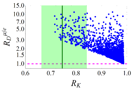
Figure 2: $R_{D}\equiv R_{D}^{\tau/\ell}$ (left panel) and $R_{D}^{\mu/e}$ (right panel) are plotted against $R_{K}$. The allowed points are compared with the experimental values (gray and green bands) at $1\sigma$. The dashed magenta line on the right panel corresponds to the SM prediction for $R_{D}^{\mu/e}\simeq 0.995$. The theory error bars for $R_{D}$ are not shown on the left panel. They are estimated to be of the order of a few percent.

There are several sources of disagreement between the present paper and Ref. [21], which we comment on in detail. First of all, their best fit values for $R_{D^{(\ast)}}$ were obtained in a setup where NP only couples to $\tau$’s. This assumption is not justified, since a putative explanation of $R_{K}$ through loops necessarily requires large couplings to muons, which then modifies the denominator in $R_{D}$, and produces excessively large $R_{D}^{\mu/e}$, as discussed above. Secondly, the conditions for the LQ parameters given by Eqs. (12) and (17) of Ref. [21] are necessary but not sufficient to reproduce results consistent with $\mathcal{B}(B\to K\nu\nu)^{\mathrm{exp}}$ and $R_{K}^{\mathrm{exp}}$, respectively. Finally, the bounds from processes involving the up-quark, such as $K\to\mu{\nu}$, $D_{s}\to(\mu,\tau){\nu}$ and $B\to\tau{\nu}$, have been tacitly neglected in their work. As mentioned before, one cannot completely avoid the first quark generation, see Eq. (22).

5 Results and discussion

In this section we present our predictions for the remaining viable scenarios, namely the LQ models ${\bm{\Delta}}^{(1/6)}$ and $\bm{U}_{3}$.

Observable	Eqs. - ${\bm{\Delta}}^{(1/6)}$	Eqs. - $\Delta^{(1/3)}$	Eqs. - $\bm{U}_{3}$	Exp. value	Ref.
$b\to s\mu\mu$	(10)	(12)	(36)	Eqs. (19)-(21)	–
$\Delta m_{B_{s}}/\Delta m_{B_{s}}^{\mathrm{SM}}$	(30)	(23)	–	1.02(10)	[47]
$R_{\nu\nu}$	(31)	(31)	(52)	$<4.3$	[45, 46]
$\mathcal{B}(\tau\to\mu\gamma)$	(42)	(44)	–	$<4.4\times 10^{-8}$	[49]
$\mathcal{B}(\tau\to\mu\phi)$	(40)	–	(54)	$<8.4\times 10^{-8}$	[47]
$\mathcal{B}(D^{0}\to\mu^{+}\mu^{-})$	–	(45)	(53)	$<7.6\times 10^{-9}$	[50]
$\mathcal{B}(K\to\mu{\nu})$	–	(25)-(27), (46)	(37),(46)	$63.58(11)\times 10^{-2}$	[51]
$\mathcal{B}(D_{s}\to\mu{\nu})$	–	(25)-(27), (46)	(37),(46)	$5.56(25)\times 10^{-3}$	[47]
$\mathcal{B}(D_{s}\to\tau{\nu})$	–	(25)-(27), (46)	(37),(46)	$5.54(24)\times 10^{-2}$	[47]
$\mathcal{B}(B\to\tau{\nu})$	–	(25)-(27), (46)	(37),(46)	$1.44(32)\times 10^{-4}$	[52, 53]
$R_{D}$	–	(25)-(27), (• ‣ A.1)	(37),(• ‣ A.1)	0.41(5)	[11, 12]

Table 1: Observables considered in our phenomenological analyses and their corresponding experimental values (or bounds) as well as their theoretical expressions for the scenarios ${\bm{\Delta}}^{(1/6)}$, $\Delta^{(1/3)}$ and $\bm{U}_{3}$.

5.1 ${\Delta}^{(1/6)}\equiv(3,2)_{1/6}$

In our analysis of the ${\bm{\Delta}}^{(1/6)}$-model we assume the LQ couplings to the first generation of fermions to be negligible because they are most tightly constrained by the experimental limits on $\mu-e$ conversion on nuclei, on atomic parity violation, on $\mathcal{B}(K_{L}\to\mu e)$, and on $\mathcal{B}(B_{s}\to\mu e)$. Therefore, the matrix of couplings $(g_{L})_{ij}$ in Eq. (7) is assumed to have the form

$$g_{L}=\begin{pmatrix}0&0&0\\ 0&(g_{L})_{s\mu}&(g_{L})_{s\tau}\\ 0&(g_{L})_{b\mu}&(g_{L})_{b\tau}\end{pmatrix},$$ (29)

where the entries are considered to be real. The product $(g_{L})_{s\mu}(g_{L})_{b\mu}^{\ast}\neq 0$ is then fixed by Eqs. (8) and (19). To constrain the couplings to $\tau$’s we use the information from $B_{s}-\bar{B_{s}}$ mixing amplitude, and the experimental limits on $\mathcal{B}(B\to K\nu\nu)$ and on $\mathcal{B}(\tau\to\mu\phi)$, see also Tab. 1. To that end we recall the expression for the mass difference of the $B_{s}-\bar{B}_{s}$ system with respect to the SM one,

$$\frac{\Delta m_{B_{s}}^{\mathrm{th}}}{\Delta m_{B_{s}}^{\mathrm{SM}}}=1+\frac{\eta_{1}(g_{L}\cdot g_{L}^{\dagger})^{2}_{bs}}{16G_{F}^{2}m_{W}^{2}|V_{tb}V_{ts}^{\ast}|^{2}\eta_{B}S_{0}(x_{t})m_{\Delta}^{2}},$$ (30)

where $(g_{L}\cdot g_{L}^{\dagger})$ denotes the product of matrices defined in Eq. (29). The ratio $R_{\nu\nu}\equiv\mathcal{B}(B\to K\nu\nu)_{\mathrm{th}}/\mathcal{B}(B\to K\nu\nu)_{\mathrm{SM}}$, in this model, is modified as follows:

$$R_{\nu\nu}=1-\frac{1}{6\,C_{L}^{\mathrm{SM}}}\mathrm{Re}\left[\dfrac{(g_{L}\cdot g_{L}^{\dagger})_{sb}}{Nm_{\Delta}^{2}}\right]+\frac{1}{48(C_{L}^{\mathrm{SM}})^{2}}\dfrac{(g_{L}\cdot g_{L}^{\dagger})_{ss}(g_{L}\cdot g_{L}^{\dagger})_{bb}}{|N|^{2}m_{\Delta}^{4}},$$ (31)

where $N={G_{F}V_{tb}V_{ts}^{\ast}\alpha_{\mathrm{em}}}/{(\sqrt{2}\pi)}$ in the case of $\Delta^{(1/6)}$ and $N=-{G_{F}V_{tb}V_{ts}^{\ast}\alpha_{\mathrm{em}}}/{(\sqrt{2}\pi)}$ in the case of $\Delta^{(1/3)}$. The SM contribution is contained in $C_{L}^{\mathrm{SM}}=-6.38(6)$ as defined in Ref. [23]. Finally, the experimental bound $\mathcal{B}(\tau\to\mu\phi)^{\mathrm{exp}}<8.4\times 10^{-8}$ [47] implies the relation

$$\frac{|(g_{L})_{s\tau}(g_{L})_{s\mu}^{\ast}|}{m_{\Delta}^{2}}<0.036\,\ \mathrm{TeV}^{-2}\quad(90\%\,\mathrm{CL}),$$ (32)

which was derived using the expression given in Appendix A.1.

Other observables, such as leptonic decays of $\phi(nS)$ and $\Upsilon(nS)$ mesons, could in principle provide useful bonds on the LQ couplings but the derived limits turn out to be much less significant at this point. Flavor conserving leptonic decays, such as $\Upsilon(nS)\to\tau\tau$, are dominated by the very large tree-level electromagnetic contribution which undermines their sensitivity to NP. LFV modes, such as $\Upsilon\to\mu\tau$, are in principle sensitive to the LQ contribution but the current experimental limit $\mathcal{B}(\Upsilon(1S)\to\mu\tau)^{\mathrm{exp}}<6\times 10^{-6}$ [54] is still too weak to be useful. We have also checked that in this model the upper experimental limit on $\mathcal{B}(\tau\to\mu\gamma)$ does not provide any additional constraint because of the cancellation of terms $\propto 1/m_{\Delta}^{2}$ in the loop function, see Eq. (42) in Appendix A.1.

Quantity	$m_{\Delta}=1$ TeV	$m_{\Delta}=5$ TeV	$m_{\Delta}=10$ TeV
$\mathcal{B}(B_{s}\to\mu\tau)$	$<1.0\times 10^{-5}$	$<3.0\times 10^{-6}$	$<1.8\times 10^{-7}$
$\mathcal{B}(B\to K\mu\tau)$	$<1.1\times 10^{-5}$	$<3.4\times 10^{-6}$	$<2.0\times 10^{-7}$
$\mathcal{B}(B\to K^{\ast}\mu\tau)$	$<2.0\times 10^{-5}$	$<6.1\times 10^{-6}$	$<3.7\times 10^{-7}$

Table 2: Predictions for exclusive $B_{(s)}$ meson decays at 90% CL for the ${\bm{\Delta}}^{(1/6)}$-model.

Using the constraints discussed above, and summarized in Tab. 1, in addition to the perturbativity prerequisite, which we here decide to be $|(g_{L})_{ij}|\leq 1$, we were able to scan the parameter space and find points which are consistent with all the requirements. With the points selected in that way, we then compute the Wilson coefficients $(C_{9}^{\mu\tau})^{\prime}=-(C_{10}^{\mu\tau})^{\prime}$ by using Eq. (8), and then insert them into Eqs. (A.3.1),(A.3.2) and (61) to compute the branching fractions. The resulting values (upper bounds) are listed in Tab. 2. Notice that the ratios of the exclusive LFV modes in this model are independent of the Wilson coefficients and given by

$$\dfrac{\mathcal{B}(B\to K^{\ast}\mu\tau)}{\mathcal{B}(B\to K\mu\tau)}\approx 1.8\qquad\quad\mathrm{and}\qquad\quad\dfrac{\mathcal{B}(B_{s}\to\mu\tau)}{\mathcal{B}(B\to K\mu\tau)}\approx 0.9,$$ (33)

where in evaluating the above ratios we used the central values of the hadronic parameters. Since most flavor observables are studied at tree-level, our predictions depend only on the ratios $(g_{L})_{d^{\prime}\ell}/m_{\Delta}$ with $d^{\prime}=d,s,b$ and $\ell=\mu,\tau$. The only exception is $\Delta m_{B_{s}}$, which exhibits a mild dependence on $m_{\Delta}$. We see from the results presented in Tab. 2 that the bounds become tighter for larger $m_{\Delta}$ which is a consequence of the condition $|(g_{L})_{ij}|\leq 1$.

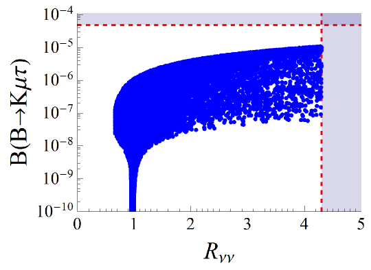
Figure 3: $\mathcal{B}(B\to K\mu\tau)$ is plotted against $R_{\nu\nu}=\mathcal{B}(B\to K\nu\nu)_{\mathrm{th}}/\mathcal{B}(B\to K\nu\nu)_{\mathrm{SM}}$ for the ${\bm{\Delta}}^{(1/6)}$-model. The blue points are allowed by flavor observables, and the red dashed lines correspond to the current experimental bounds $R_{\nu\nu}^{\mathrm{exp}}<4.3$ [46] and $\mathcal{B}(B^{+}\to K^{+}\mu^{\pm}\tau^{\mp})^{\mathrm{exp}}<4.8\times 10^{-5}$ [7].

We next check on the correlation between $\mathcal{B}(B\to K\mu\tau)$ and $R_{\nu\nu}$ for a benchmark $m_{\Delta}=1$ TeV. We see from Fig. 3 that the compatibility of $R_{\nu\nu}$ with the SM value, $R^{\rm SM}_{\nu\nu}=1$, would not exclude the possibility of rather large branching fractions for the LFV decay modes. However, if the value of $R_{\nu\nu}$ is found to be significantly below or above $1$ then this analysis provides both an upper and a lower bound for $\mathcal{B}(B\to K\tau\mu)$. For example, if $R_{\nu\nu}\approx 2$, we get

$$2\times 10^{-8}\lesssim\mathcal{B}(B\to K\mu\tau)\lesssim 5\times 10^{-6}.$$ (34)

Furthermore, we see that the current experimental bound, $R_{\nu\nu}^{\mathrm{exp}}\leq 4.3$, is an efficient constraint but it ceases to be so if we consider $m_{\Delta}\gtrsim 3$ TeV. Finally, it is interesting to note that the BaBar bound, $\mathcal{B}(B\to K\mu\tau)^{\mathrm{exp}}<4.8\times 10^{-5}$, is only an order of magnitude larger than the upper bound we obtained in our analysis. We hope that the high statistics LHCb data, and especially those of the future Belle II, will be used to improve this as well as other bounds on similar decay modes. We reiterate that a bound on any of the modes considered above would be equally useful, since they are all related to each other through the ratios given in Eq. (33). Before closing this part of our analysis, we should mention that this LQ model has been extended to accommodate $R_{D}^{\rm exp}$ in Ref. [55], without changing the upper bounds on the LFV rates discussed in this paper but providing the lower ones which are $\mathcal{O}(10^{-10})$.

5.1.1 Comment on $B_{s}\to\tau\tau$

Since the LHCb Collaboration is actively searching for the $B_{s}\to\tau\tau$ events, we also show the correlation between $\mathcal{B}(B\to K\mu\tau)$ and $\mathcal{B}(B_{s}\to\tau\tau)$ in Fig. 4. We see again that even if $\mathcal{B}(B_{s}\to\tau\tau)$ is found to be consistent with the SM value, $\mathcal{B}(B_{s}\to\tau\tau)^{\rm SM}=7.7(5)\times 10^{-7}$, one can still have a significant $\mathcal{B}(B\to K\mu\tau)$. This can be understood from Eq. (8), since $B_{s}\to\tau\tau$ will be modified by NP only if the product $(g_{L})_{s\tau}(g_{L})_{b\tau}^{\ast}$ is nonzero, and therefore one should have both $(g_{L})_{s\tau}\neq 0$ and $(g_{L})_{b\tau}\neq 0$ to produce a deviation from the SM. On the other hand, the product $(g_{L})_{s\mu}(g_{L})_{b\mu}^{\ast}$ is already fixed to a nonzero value by $b\to s\mu\mu$ exclusive data. Therefore, it is enough to have one of the couplings $(g_{L})_{s\tau}$ or $(g_{L})_{b\tau}$ different from zero in order to induce LFV in $B_{(s)}$ decays through the effective coefficients $(C_{10}^{\tau\mu})^{\prime}$ or $(C_{10}^{\mu\tau})^{\prime}$, respectively. For that reason, the LFV modes are more robust probes of the LQ couplings. Notice, however, that if LHCb can establish an upper bound on $\mathcal{B}(B_{s}\to\tau\tau)$, this would certainly be more important than the other limits that we have used here to constraint the third generation couplings.

If, instead, the measured $\mathcal{B}(B_{s}\to\tau\tau)$ turns out to be larger or smaller than $\mathcal{B}(B_{s}\to\tau\tau)^{\rm SM}$ this model offers also a lower bound on $\mathcal{B}(B\to K\mu\tau)$, which is quite remarkable because in this way one can check the validity of this scenario. Moreover, we see also that if $\mathcal{B}(B_{s}\to\tau\tau)\gtrsim 2\times 10^{-5}$ is measured then this model not only cannot generate LFV, but it will be ruled out altogether.

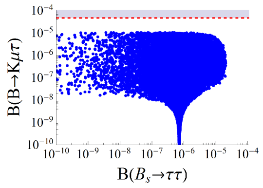
Figure 4: $\mathcal{B}(B\to K\mu\tau)$ is plotted against $\mathcal{B}(B_{s}\to\tau\tau)$ for the ${\bm{\Delta}}^{(1/6)}$-model. See Fig. 3 for details.

5.2 ${U_{3}}\equiv(3,3)_{2/3}$

In a UV-complete renormalizable model containing $\bm{U}_{3}$ at the lower end of the spectrum (and possibly accompanying light degrees of freedom), we expect the $3\times 3$ matrix of LQ couplings $x^{LL}$ in Eq. (16) to be unitary. Indeed, if $\bm{U}_{3}$ was a remnant of a larger multiplet of gauge bosons, one could consider a theory in the unitary gauge in which the UV divergences appearing in the flavour changing neutral processes are removed by the sums over the couplings, i.e. by the GIM mechanism, and for this technique to work we would require $x^{LL}$ to be unitary.  However, in the unitary case the couplings to $e$ and/or first generation of quarks cannot be avoided and then the very strong null constraints from LFV searches apply. In this particular case, we have found that the upper bounds on $\mu-e$ conversion on Au nucleus and the one on ${\cal B}(K_{L}\to\mu e)$ already discard $\bm{U}_{3}$ with unitary $x^{LL}$ as a viable scenario for explaining $R_{K}^{\rm exp}$.

Thus we continue along with our analysis using the non-unitary ansatz, and we completely avoid couplings to electrons by paying the price of being unable to unambiguously predict any loop-induced process. The ansatz below couples only the second and third generation charged leptons with the down-type quarks. However, as before, the CKM rotation will induce the couplings of $u,c,t$ to the charged leptons and neutrinos, viz.

$$x^{LL}=\begin{pmatrix}0&0&0\\ 0&x^{LL}_{s\mu}&x^{LL}_{s\tau}\\ 0&x^{LL}_{b\mu}&x^{LL}_{b\tau}\end{pmatrix},\qquad Vx^{LL}=\begin{pmatrix}0&V_{us}x^{LL}_{s\mu}+V_{ub}x^{LL}_{b\mu}&V_{us}x^{LL}_{s\tau}+V_{ub}x^{LL}_{b\tau}\\ 0&V_{cs}x^{LL}_{s\mu}+V_{cb}x^{LL}_{b\mu}&V_{cs}x^{LL}_{s\tau}+V_{cb}x^{LL}_{b\tau}\\ 0&V_{ts}x^{LL}_{s\mu}+V_{tb}x^{LL}_{b\mu}&V_{ts}x^{LL}_{s\tau}+V_{tb}x^{LL}_{b\tau}\end{pmatrix}.$$ (35)

Observables that constrain this LQ have already been discussed in Ref. [20]. Left-handed couplings of $U_{3\mu}^{(2/3)}$ alone allow for a single combination of the Wilson coefficients:

$$C_{9}^{\ell_{1}\ell_{2}}=-C_{10}^{\ell_{1}\ell_{2}}=-\frac{\pi v^{2}}{V_{tb}V_{ts}^{\ast}\alpha_{\mathrm{em}}m_{U}^{2}}x^{LL}_{s\ell_{2}}x_{b\ell_{1}}^{LL\ast}.$$ (36)

As discussed in Sec. 4.1, by using the measured $\mathcal{B}(B_{s}\to\mu^{+}\mu^{-})^{\rm exp}$ and $\mathcal{B}(B\to K\mu^{+}\mu^{-})_{\text{high}-q^{2}}^{\rm exp}$, we select the values of $C_{9}^{\mu\mu}=-C_{10}^{\mu\mu}$, to $2\sigma$ accuracy and obtain $C_{9}^{\mu\mu}\in(-0.76,-0.04)$, cf. Eq. (21). It is interesting to note that $\mathcal{B}(B_{s}\to\mu^{+}\mu^{-})^{\rm exp}$ and $R_{K}^{\rm exp}$ impose almost degenerate constraints on $C_{9}^{\mu\mu}$. For example, the result for $C_{9}^{\mu\mu}=-C_{10}^{\mu\mu}$ to $1\sigma$, results in $R_{K}\in(0.74,0.88)$, which fully agrees with $R_{K}^{\rm exp}$.

The three charge components of $\bm{U}_{3}$, with the same underlying couplings, allow for flavor effects both in the down/up-quarks and the charged lepton/neutrino sectors. Interestingly, the $2/3$-charge component plays an important role in the charged current semileptonic processes and thus can be used to address the hint of LFU violation in $R_{D^{(*)}}$. Using the effective Lagrangian parametrization of the charged current (24) the left-handed current modification reads

$$g_{V}\big{|}_{b\to c\ell{\nu}_{\ell^{\prime}}}=-\frac{1}{2\sqrt{2}G_{F}V_{cb}}\frac{x^{LL*}_{b\ell}(Vx^{LL})_{c\ell^{\prime}}}{m_{U}^{2}}.$$ (37)

Through $g_{V}$ the $\bm{U}_{3}$ vector LQ state modifies the overall normalization of the SM spectrum of $B\to D\ell\bar{\nu}$ without modifying its shape, cf. Eq. (• ‣ A.1) in Appendix A.

Thus in the $\bm{U}_{3}$-model we vary the couplings within $|x^{LL}_{ij}|<4\pi$ and apply the above-mentioned constraints, namely the one on $C_{9}^{\mu\mu}$, and the one arising from $R_{D}^{\mathrm{exp}}$, both at $2\sigma$.  We fix the mass at $m_{U}=1$ TeV. Further constraints are coming from the purely third-generation charged current and the up-type neutral current processes which are mediated by the $U_{3\mu}^{(5/3)}$ eigencharge component. Among the charged current processes, the most efficient constraint comes from the measured ${\cal B}(t\to b\tau\nu)^{\mathrm{exp}}=0.096(28)$ [63]. The effect of $\bm{U}_{3}$ here is an overall rescaling of $t\to b\tau\nu$ via coupling $g_{V}|_{b\to t\tau\nu_{\ell^{\prime}}}$, cf. Eq. (37). We apply this constraint by eliminating any point in the parameter space that results in ${\cal B}(t\to b\tau\nu)$ out of the $1\sigma$ region of ${\cal B}(t\to b\tau\nu)^{\mathrm{exp}}$. Once the above constraints are applied it appears that the constraints coming from the up-quark rare process, $\mathcal{B}(D^{0}\to\mu\mu)^{\mathrm{exp}}<6.2\times 10^{-9}$ [47] (cf. Eq. (53)), and from ${\cal B}(\tau\to\mu\phi)$ are redundant. Furthermore, we have checked that the LFU ratios, $\Gamma(\tau\to K\nu)/\Gamma(K\to\mu\nu)$ and $\Gamma(K\to\mu\nu)/\Gamma(K\to e\nu)$, are consistent with experiment.

Like in the previous subsection, with the couplings selected to verify the above constraints, we can compute various quantities. In particular, in Fig. 5 we show the correlation between $R_{\nu\nu}$ and ${\cal B}(B_{s}\to\tau\tau)$, and again observe that the current experimental limit on $R_{\nu\nu}$ provides a stringent constraint on the parameter space. Note that $B\to K\nu\nu$ is governed by the $Q=-1/3$ component which connects the down-type quarks to neutrinos.

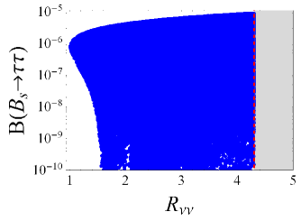
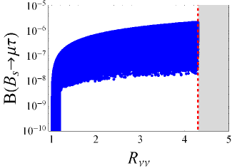
Figure 5: Correlation between $R_{\nu\nu}$ and ${\cal B}(B_{s}\to\tau\tau)$ in the $\bm{U}_{3}$-model ($m_{U}=1$ TeV). The shaded grey region is excluded at 90% CL by the upper experimental bound on $R_{\nu\nu}$.

Finally, on the right panel of Fig. 5 we show ${\cal B}(B_{s}\to\mu\tau)$ with respect to $R_{\nu\nu}$, and we see that this model allows for large LFV decay branching fractions even if $R_{\nu\nu}$ and ${\cal B}(B_{s}\to\tau\tau)$ are close to their SM values. We obtain

$${\cal B}(B_{s}\to\mu\tau)\lesssim 2.7\times 10^{-6},$$ (38)

for ${m_{U}}\simeq 1$ TeV. The bounds on the other two LFV modes can be obtained by simply using Eq. (33), i.e.

$$\mathcal{B}(B\to K\mu\tau)\lesssim 3\times 10^{-6},\qquad\mathcal{B}(B\to K^{\ast}\mu\tau)\lesssim 5.4\times 10^{-6}.$$ (39)

The strong correlation between LFV and bi-neutrino modes is a signature of this model, should positive LFV signal or $R_{\nu\nu}>1$ emerge. On the other hand, for the $B_{s}\to\tau\tau$ mode the left-hand panel in Fig. 5 demonstrates that it can be larger by about an order of magnitude than its SM prediction. For $R_{\nu\nu}>1$ there is a possibility of strong suppression of $\mathcal{B}(B_{s}\to\tau\tau)$. Finally, the observation of $R_{\nu\nu}$ significantly smaller than $1$ is not compatible with the presence of $\bm{U}_{3}$ as an explanation for $R_{K}^{\mathrm{exp}}$ and $R_{D}^{\mathrm{exp}}$. We should emphasise that all the observables considered in this section have identical scaling with $\bm{U}_{3}$ couplings and mass, thus the correlations presented in Fig. 5 are kept intact for different choices of $m_{U}$, with the exception of perturbativity constraints which are becoming more stringent for increasing $m_{U}$.

6 Summary

In this paper we discuss exclusive $b\to s\ell_{1}\ell_{2}$ LFV decay modes in various models in which the existence of an $\mathcal{O}(1\ {\rm TeV})$ leptoquark state is assumed. In doing so we use the effective field theory approach and derive the expressions for the Wilson coefficients in each of the considered scenarios, which then allows us to test them against the available experimental data for $\mathcal{B}(B_{s}\to\mu^{+}\mu^{-})^{\rm exp}$ and $\mathcal{B}(B\to K\mu^{+}\mu^{-})^{\rm exp}$ at large $q^{2}$, and select those which lead to predictions of other processes that are consistent with current experimental data. These two quantities are used mostly because the theoretical uncertainties are under better control since the hadronic matrix elements have been estimated by means of numerical simulations of QCD on the lattice, and also because the high-$q^{2}$ region is above the very narrow $c\bar{c}$-resonances, so that the contribution of $c\bar{c}$ can be treated by using the quark-hadron duality.

We find that two models (scenarios), compatible with the above-mentioned experimental constraints, can accommodate the experimental hint on LFU violation, namely $R_{K}^{\rm exp}=\mathcal{B^{\prime}}(B^{+}\to K^{+}\mu\mu)/\mathcal{B^{\prime}}(B^{+}\to K^{+}ee)<R_{K}^{\rm SM}$, and that they lead to the results in other processes that are compatible with experiment (and with the measured $\Delta m_{B_{s}}^{\mathrm{exp}}$, in particular). Moreover, we find that the current experimental bound $R_{\nu\nu}^{\mathrm{exp}}$ is particularly useful in cutting a significant fraction of the parameter space. The two scenarios that we select as plausible are:

• Scenario with ${\bm{\Delta}}^{(1/6)}$, a doublet of (mass degenerate) scalar leptoquarks of hypercharge $Y=1/6$, for which the NP contribution to $\mathcal{B}(B_{s}\to\mu^{+}\mu^{-})$ and $\mathcal{B}(B\to K\mu^{+}\mu^{-})$ comes from the left-handed couplings, and for which the bound $\mathcal{B}(\tau\to\phi\mu)^{\rm exp}$ appears to be useful. Interestingly, we find that the LFV mode $\mathcal{B}(B\to K\mu\tau)$ can go up to $\mathcal{O}(10^{-6})$ even if $R_{\nu\nu}=1$ and $\mathcal{B}(B_{s}\to\tau\tau)^{\rm exp}=\mathcal{B}(B_{s}\to\tau\tau)^{\rm SM}$, but that it is strictly different from zero for $R_{\nu\nu}\neq 1$ and $\mathcal{B}(B_{s}\to\tau\tau)^{\rm exp}\neq\mathcal{B}(B_{s}\to\tau\tau)^{\rm SM}$. For example, for $R_{\nu\nu}\approx 2$, in this model we get $\mathcal{B}(B\to K\mu\tau)\in(0.2,50)\times 10^{-7}$. Notice that this model is experimentally verifiable: (i) it leads to $R_{K^{\ast}}>1$ [19], and (ii) it does not allow $R_{\nu\nu}\lesssim 0.6$, nor $\mathcal{B}(B_{s}\to\tau\tau)\gtrsim 2\times 10^{-5}$.

• Scenario with $\bm{U}_{3}$, a triplet of (mass degenerate) vector leptoquarks of hypercharge $Y=2/3$, for which the NP contribution to $\mathcal{B}(B_{s}\to\mu^{+}\mu^{-})$ and $\mathcal{B}(B\to K\mu^{+}\mu^{-})$ comes from the left handed couplings, and for which the bound on $R_{\nu\nu}^{\rm exp}$ as well as $\mathcal{B}(t\to b\tau\nu)^{\rm exp}$ provide the crucial constraints on its Yukawa couplings. Like in the previous case, the branching ratio $\mathcal{B}(B\to K\mu\tau)$ can be between zero and $\mathcal{O}(10^{-6})$ even if $R_{\nu\nu}=1$ and $\mathcal{B}(B_{s}\to\tau\tau)^{\rm exp}=\mathcal{B}(B_{s}\to\tau\tau)^{\rm SM}$, but it is stricly non-zero for $R_{\nu\nu}>1$. This model too is experimentally verifiable: (i) it leads to $R_{K^{\ast}}=0.86(12)$, thus $R_{K^{\ast}}<1$ [41], and (ii) it can be ruled out if $R_{\nu\nu}<1$ and/or $\mathcal{B}(B_{s}\to\tau\tau)\gtrsim 10^{-5}$.

As for the branching fractions of the similar LFV decay modes, they are related to $\mathcal{B}(B\to K\mu\tau)$ via Eq. (33), as discussed in Ref. [24]. Notice that we also examined the model with a singlet scalar leptoquark of hypercharge $Y=-1/3$ and found that it is not phenomenologically viable, i.e. that it cannot accommodate $R_{K}<1$ without running into serious phenomenological difficulties with other measured processes.

Acknowledgments: We would like to thank S. Fajfer for discussions, and P. Arnan for pointing out to us the subtlety related to the interference term in Eq. (31) of the present paper. R.Z.F. thanks the Université Paris Sud for the kind hospitality, and CNPq and FAPESP for partial financial support. N.K. acknowledges support of the Slovenian Research Agency. This project has received funding from the European Union’s Horizon 2020 research and innovation program under the Marie Sklodowska-Curie grant agreement No. 674896.

Appendix A Formulas and hadronic quantities

In this Appendix we collect the expressions and numerical values used in our analyses.

A.1 Scalar Leptoquarks

• $\tau\to\mu\phi$: We use the experimental upper bound $\mathcal{B}(\tau\to\mu\phi)<8.4\times 10^{-8}$ [47], and the expression we derived,

  $$\mathcal{B}(\tau\to\mu\phi)=\frac{f_{\phi}^{2}m_{\phi}^{4}}{256\pi m_{\tau}^{3}\Gamma_{\tau}}\left|\frac{g_{s\tau}g_{s\mu}^{\ast}}{m_{\Delta}^{2}}\right|^{2}\left[-1+\frac{(m_{\mu}^{2}+m_{\tau}^{2})}{2m_{\phi}^{2}}+\frac{(m_{\mu}^{2}-m_{\tau}^{2})^{2}}{2m_{\phi}^{4}}\right]\lambda^{1/2}(m_{\phi}^{2},m_{\tau}^{2},m_{\mu}^{2}),$$ (40)

  where the couplings $g_{s\ell}$ can be either $(g_{L})_{s\ell}$ for the model ${\bm{\Delta}}^{(1/6)}=(3,2)_{1/6}$, or $(g_{R})_{s\ell}$ if the model ${\bm{\Delta}}^{(7/6)}=(3,2)_{7/6}$ is considered.

• $\tau\to\mu\gamma$: We use the upper bound $\mathcal{B}(\tau\to\mu\gamma)<4.4\times 10^{-8}$ [49], and the expression

  $$\mathcal{B}(\tau\to\mu\gamma)=\frac{\alpha_{\mathrm{em}}(m_{\tau}^{2}-m_{\mu}^{2})^{3}}{4m_{\tau}^{3}\Gamma_{\tau}}\left(|\sigma_{L}|^{2}+|\sigma_{R}|^{2}\right),$$ (41)

  where the coefficients $\sigma_{L(R)}$ for the models ${\bm{\Delta}}^{(1/6)}$, ${\bm{\Delta}}^{(7/6)}$ and $\Delta^{(1/3)}$, to leading order in $1/m_{\Delta}$, read [4, 57]

  $$\sigma_{L}^{(1/6)} =0,\qquad\sigma_{R}^{(1/6)}=-i(g_{L})_{b\mu}(g_{L})_{b\tau}^{\ast}\frac{N_{C}m_{b}^{2}m_{\tau}}{96\pi^{2}m_{\Delta}^{4}}\left[\frac{5}{2}+\log\left(\frac{m_{b}^{2}}{m_{\Delta}^{2}}\right)\right],$$ (42)

  $$\sigma_{R}^{(7/6)} =0,\qquad\sigma_{L}^{(7/6)}=i(g_{R})_{b\mu}(g_{R})_{b\tau}^{\ast}\frac{N_{C}m_{\tau}}{64\pi^{2}m_{\Delta}^{2}}\left\{1+\frac{4}{3}\frac{m_{t}^{2}}{m_{\Delta}^{2}}\left[1+\log\left(\frac{m_{t}^{2}}{m_{\Delta}^{2}}\right)\right]\right\},$$ (43)

  $$\sigma_{L(R)}^{(1/3)} =-i\frac{N_{C}m_{\tau}}{192\pi^{2}m_{\Delta}^{2}}\Bigg{\{}(g_{R(L)})_{t\tau}(g_{R(L)})_{t\mu}^{\ast}-\frac{m_{t}}{m_{\tau}}(g_{L(R)})_{t\tau}(g_{R(L)})_{t\mu}^{\ast}\Bigg{[}14+8\log\left(\frac{m_{t}^{2}}{m_{\Delta}^{2}}\right)\Bigg{]}\Bigg{\}},$$ (44)

  with $N_{C}=3$ and $(g_{L(R)})_{u\ell}=\sum_{d}V_{ud}^{\ast}(g_{L(R)})_{d\ell}$ in the last equation, where $u(d)$ stand for generic up(down)-type quark flavors.

• $D^{0}\to\mu^{+}\mu^{-}$: We use the experimental limit $\mathcal{B}(D^{0}\to\mu^{+}\mu^{-})<7.6\times 10^{-9}$ ($95\%$ CL) [50] and the expression [21]

  $$\mathcal{B}(D^{0} \to\mu^{+}\mu^{-})=\frac{f_{D}^{2}m_{D}^{3}}{256\pi m_{\Delta}^{4}\Gamma_{D}}\left(\frac{m_{D}}{m_{c}}\right)^{2}\beta_{\mu}\Bigg{[}\beta_{\mu}^{2}\left|(g_{L})_{c\mu}(g_{R})_{u\mu}^{\ast}-(g_{R})_{c\mu}(g_{L})_{u\mu}^{\ast}\right|^{2}$$ (45)

  $$+\left|(g_{L})_{c\mu}(g_{R})_{u\mu}^{\ast}+(g_{R})_{c\mu}(g_{L})_{u\mu}^{\ast}+\frac{2m_{\mu}m_{c}}{m_{D}^{2}}\left[(g_{L})_{c\mu}(g_{L})_{u\mu}^{\ast}+(g_{R})_{c\mu}(g_{R})_{u\mu}^{\ast}\right]\right|^{2}\Bigg{]},$$

  where $m_{c}=m_{c}(m_{\Delta})$ is the running charm quark mass.

• $B\to\tau\nu$  and $B\to D\tau\nu$: Using the effective Lagrangian defined in Eq. (24) one can compute the leptonic and semileptonic decay rates for the specific channels, e.g. for $B\to D\ell\nu_{\ell^{\prime}}$ and $B\to\ell\nu_{\ell^{\prime}}$. We obtain

  $$\Gamma(B\to\ell\nu_{\ell^{\prime}}) =\frac{G_{F}^{2}m_{B}|V_{ub}|^{2}}{8\pi}f_{B}^{2}m_{\ell}^{2}\left(1-\frac{m_{\ell}^{2}}{m_{B}^{2}}\right)^{2}\left|\delta_{\ell\ell^{\prime}}+g_{V}-g_{S}(\mu)\frac{m_{B}^{2}}{m_{\ell}(m_{c}+m_{b})}\right|^{2},$$ (46)

  and

  $$\dfrac{\mathrm{d}\Gamma}{\mathrm{d}q^{2}}(B\to D\ell\nu_{\ell^{\prime}})=\frac{G_{F}^{2}|V_{cb}|^{2}}{192\pi^{3}m_{B}^{3}} |f_{+}(q^{2})|^{2}\Bigg{\{}|\delta_{\ell\ell^{\prime}}+g_{V}|^{2}c_{+}^{\ell}(q^{2})+|g_{T}(\mu)|^{2}c_{T}^{\ell}(q^{2})\left|\frac{f_{T}(q^{2})}{f_{+}(q^{2})}\right|^{2}$$

  $$+c_{TV}^{\ell}(q^{2})\,\mathrm{Re}\left[(\delta_{\ell\ell^{\prime}}+g_{V})g_{T}^{\ast}(\mu)\right]\frac{f_{T}(q^{2},\mu)}{f_{+}(q^{2})}$$

  $$+c_{0}^{\ell}(q^{2})\left|\delta_{\ell\ell^{\prime}}+g_{V}+g_{S}(\mu)\frac{q^{2}}{m_{\ell}(m_{d}-m_{u})}\right|^{2}\left|\frac{f_{0}(q^{2})}{f_{+}(q^{2})}\right|^{2}\Bigg{\}},$$ (47)

  where we emphasize that the NP contribution can allow for a different neutrino flavor $\ell\neq\ell^{\prime}$ in the final state. The $B\to D$ form factors and the $f_{B}$ decay constant are defined in the Appendix A.3, and the phase-space functions $c_{i}^{\ell}(q^{2})$ are given by [15]

  $$c_{+}^{\ell}(q^{2}) =\lambda^{3/2}(\sqrt{q^{2}},m_{B},m_{D})\left[1-\frac{3}{2}\frac{m_{\ell}^{2}}{q^{2}}+\frac{1}{2}\left(\frac{m_{\ell}^{2}}{q^{2}}\right)^{3}\right],$$ (48)

  $$c_{0}^{\ell}(q^{2}) =m_{\ell}^{2}\,\lambda^{1/2}(\sqrt{q^{2}},m_{B},m_{D})\dfrac{3}{2}\dfrac{m_{B}^{4}}{q^{2}}\left(1-\dfrac{m_{\ell}^{2}}{q^{2}}\right)^{2}\left(1-\dfrac{m_{D}^{2}}{m_{B}^{2}}\right)^{2},$$ (49)

  $$c_{T}^{\ell}(q^{2}) =\lambda^{3/2}(\sqrt{q^{2}},m_{B},m_{D})\frac{8q^{2}}{(m_{B}+m_{D})^{2}}\left[1-3\left(\frac{m_{\ell}^{2}}{q^{2}}\right)^{2}+2\left(\frac{m_{\ell}^{2}}{q^{2}}\right)^{3}\right],$$ (50)

  $$c_{TV}^{\ell}(q^{2}) =\frac{12m_{\ell}}{m_{B}+m_{D}}\lambda^{3/2}(\sqrt{q^{2}},m_{B},m_{D})\left(1-\frac{m_{\ell}^{2}}{q^{2}}\right)^{2},$$ (51)

  with $\lambda(a,b,c)=[a^{2}-(b+c)^{2}][a^{2}-(b-c)^{2}]$.

A.2 Vector leptoquark $U_{3}$

• $B\to K\nu\nu$: The relative modification of the SM decay rate of $B\to K\nu\nu$ in the presence of the $U_{3\mu}^{(-1/3)}$ reads [4]

  $$\begin{split}R_{\nu\nu}=1&-\frac{2}{3C_{L}^{\rm SM}}\,\mathrm{Re}\left[{(x^{LL}\cdot x^{LL{\dagger}})_{sb}\over Nm_{U}^{2}}\right]+\frac{1}{3|C_{L}^{\mathrm{SM}}|^{2}}{(x^{LL}\cdot x^{LL{\dagger}})_{ss}(x^{LL}\cdot x^{LL{\dagger}})_{bb}\over|N|^{2}m_{U}^{4}},\end{split}$$ (52)

  where $C_{L}^{\mathrm{SM}}=-6.38\pm 0.06$ [23].

• $D^{0}\to\mu^{+}\mu^{-}$: The branching ratio of the rare decay $D^{0}\to\mu\mu$ is sensitive to the CKM-rotated matrix $x^{LL}$:

  $$\Gamma_{D^{0}\to\mu\mu}=\frac{f_{D}^{2}m_{D}m_{\mu}^{2}}{8\pi}\sqrt{1-\frac{4m_{\mu}^{2}}{m_{D}^{2}}}\frac{\left|(Vx^{LL})_{u\mu}(Vx^{LL})_{c\mu}^{*}\right|^{2}}{m_{U}^{4}}.$$ (53)

• $\tau\to\mu\phi$: The expression relevant to this LFV decay mode in the $\bm{U}_{3}$-model reads,

  $$\mathcal{B}(\tau\to\mu\phi)=\frac{f_{\phi}^{2}m_{\phi}^{4}}{64\pi m_{\tau}^{3}\Gamma_{\tau}}\left|\frac{x^{LL}_{s\tau}x^{LL\ast}_{s\mu}}{m_{U}^{2}}\right|^{2}\left[-1+\frac{(m_{\mu}^{2}+m_{\tau}^{2})}{2m_{\phi}^{2}}+\frac{(m_{\mu}^{2}-m_{\tau}^{2})^{2}}{2m_{\phi}^{4}}\right]\lambda^{1/2}(m_{\phi}^{2},m_{\tau}^{2},m_{\mu}^{2}).$$ (54)

A.3 Exclusive $b\to s$ decay rates

We recall in this section the full decay rate expressions for the modes $B_{s}\to\ell_{1}\ell_{2}$ and $B\to K^{(\ast)}\ell_{1}\ell_{2}$ [24].

A.3.1 $B_{s}\to\ell_{1}\ell_{2}$

The branching fraction for the mode $B_{s}\to\ell_{1}\ell_{2}$ reads

$$\mathcal{B}(B_{s}\to \ell_{1}^{-}\ell_{2}^{+})^{\mathrm{th}}=\frac{\tau_{B_{s}}}{64\pi^{3}}\frac{\alpha_{\mathrm{em}}^{2}G_{F}^{2}}{m_{B_{s}}^{3}}f_{B_{s}}^{3}|V_{tb}V_{ts}^{\ast}|^{2}\lambda^{1/2}(m_{B_{s}},m_{1},m_{2})$$

$$\times\Bigg{\{}[m_{B_{s}}^{2}-(m_{1}+m_{2})^{2}]\cdot\Bigg{|}(C_{9}-C_{9}^{\prime})(m_{1}-m_{2})+(C_{S}-C_{S}^{\prime})\frac{m_{B_{s}}^{2}}{m_{b}+m_{s}}\Bigg{|}^{2}$$

$$\quad+[m_{B_{s}}^{2}-(m_{1}-m_{2})^{2}]\cdot\Bigg{|}(C_{10}-C_{10}^{\prime})(m_{1}+m_{2})+(C_{P}-C_{P}^{\prime})\frac{m_{B_{s}}^{2}}{m_{b}+m_{s}}\Bigg{|}^{2}\Bigg{\}},$$ (55)

where the $B_{s}$-meson decay constant $f_{B_{s}}$ is defined by $\Braket{0}{\bar{b}\gamma_{\mu}\gamma_{5}s}{B_{s}(p)}=ip_{\mu}f_{B_{s}}$.

A.3.2 $B\to K\ell_{1}\ell_{2}$

The differential branching ratio of $\bar{B}\to\bar{K}\ell_{1}^{-}\ell_{2}^{+}$ is given by

$$\dfrac{\mathrm{d}\mathcal{B}}{\mathrm{d}q^{2}}(\bar{B}\to\bar{K}\ell_{1}^{-}\ell_{2}^{+})= \left|\mathcal{N}_{K}(q^{2})\right|^{2}\times\Big{\{}\varphi_{7}(q^{2})|C_{7}+C_{7}^{\prime}|^{2}+\varphi_{9}(q^{2})|C_{9}+C_{9}^{\prime}|^{2}+\varphi_{10}(q^{2})|C_{10}+C_{10}^{\prime}|^{2}$$

$$+\varphi_{S}(q^{2})|C_{S}+C_{S}^{\prime}|^{2}+\varphi_{P}(q^{2})|C_{P}+C_{P}^{\prime}|^{2}+\varphi_{79}(q^{2})\mathrm{Re}[(C_{7}+C_{7}^{\prime})(C_{9}+C_{9}^{\prime})^{\ast}]$$

$$+\varphi_{9S}(q^{2})\mathrm{Re}[(C_{9}+C_{9}^{\prime})(C_{S}+C_{S}^{\prime})^{\ast}]+\varphi_{10P}(q^{2})\mathrm{Re}[(C_{10}+C_{10}^{\prime})(C_{P}+C_{P}^{\prime})^{\ast}]\Big{\}},$$ (56)

where $(m_{1}+m_{2})^{2}\leq q^{2}\leq(m_{B}-m_{K})^{2}$, and the explicit expressions for the phase-space functions $\varphi_{i}(q^{2})$ write

$$\varphi_{7}(q^{2}) =\frac{2m_{b}^{2}|f_{T}(q^{2})|^{2}}{(m_{B}+m_{K})^{2}}\lambda_{B}\left[1-\frac{(m_{1}-m_{2})^{2}}{q^{2}}-\frac{\lambda_{q}}{3q^{4}}\right],$$

$$\begin{split}\varphi_{9(10)}(q^{2})&=\frac{1}{2}|f_{0}(q^{2})|^{2}(m_{1}\mp m_{2})^{2}\frac{(m_{B}^{2}-m_{K}^{2})^{2}}{q^{2}}\left[1-\frac{(m_{1}\pm m_{2})^{2}}{q^{2}}\right]\\ &+\frac{1}{2}|f_{+}(q^{2})|^{2}\lambda_{B}\left[1-\frac{(m_{1}\mp m_{2})^{2}}{q^{2}}-\frac{\lambda_{q}}{3q^{4}}\right],\\[6.00006pt] \varphi_{79}(q^{2})&=\frac{2m_{b}f_{+}(q^{2})f_{T}(q^{2})}{m_{B}+m_{K}}\lambda_{B}\left[1-\frac{(m_{1}-m_{2})^{2}}{q^{2}}-\frac{\lambda_{q}}{3q^{4}}\right],\\[6.00006pt] \varphi_{S(P)}(q^{2})&=\frac{q^{2}|f_{0}(q^{2})|^{2}}{2(m_{b}-m_{s})^{2}}(m_{B}^{2}-m_{K}^{2})^{2}\left[1-\frac{(m_{1}\pm m_{2})^{2}}{q^{2}}\right],\\[6.00006pt] \varphi_{10P(9S)}(q^{2})&=\frac{|f_{0}(q^{2})|^{2}}{m_{b}-m_{s}}(m_{1}\pm m_{2})(m_{B}^{2}-m_{K}^{2})^{2}\left[1-\frac{(m_{1}\mp m_{2})^{2}}{q^{2}}\right],\end{split}$$ (57)

with $\lambda_{q}\equiv\lambda(\sqrt{q^{2}},m_{1},m_{2})$, $\lambda_{B}\equiv\lambda(\sqrt{q^{2}},m_{B},m_{K})$, and

$$\left|\mathcal{N_{K}}(q^{2})\right|^{2}=\tau_{B_{d}}\dfrac{\alpha_{\mathrm{em}}^{2}G_{F}^{2}|V_{tb}V_{ts}^{\ast}|^{2}}{512\pi^{5}m_{B}^{3}}\frac{\lambda_{q}^{1/2}\lambda_{B}^{1/2}}{q^{2}}.$$ (58)

These expressions are computed by using the (standard) parametrization of the hadronic matrix elements in terms of form factors $f_{+,0,T}(q^{2})$, namely,

$$\langle\bar{K}(k)|\bar{s}\gamma_{\mu}b|\bar{B}(p)\rangle =\left[(p+k)_{\mu}-\frac{m_{B}^{2}-m_{K}^{2}}{q^{2}}q_{\mu}\right]f_{+}(q^{2})+\dfrac{m_{B}^{2}-m_{K}^{2}}{q^{2}}q_{\mu}f_{0}(q^{2}),$$ (59)

$$\langle\bar{K}(k)|\bar{s}\sigma_{\mu\nu}b|\bar{B}(p)\rangle =-i(p_{\mu}k_{\nu}-p_{\nu}k_{\mu})\dfrac{2f_{T}(q^{2},\mu)}{m_{B}+m_{K}}.$$ (60)

A.3.3 $B\to K^{\ast}\ell_{1}\ell_{2}$

Finally, the differential branching ratio of $B\to\bar{K}^{\ast}\ell_{1}^{-}\ell_{2}^{+}$ is given by

$$\dfrac{\mathrm{d}\mathcal{B}}{\mathrm{d}q^{2}}(B\to\bar{K}^{\ast}\to(K\pi)\ell_{1}^{-}\ell_{2}^{+})=\dfrac{1}{4}\left[3I_{1}^{c}(q^{2})+6I_{1}^{s}(q^{2})-I_{2}^{c}(q^{2})-2I_{2}^{s}(q^{2})\right],$$ (61)

where the relevant angular coefficients $I_{i}(q^{2})$ read

$$I_{1}^{s}(q^{2}) =\Big{[}|A_{\perp}^{L}|^{2}+|A_{\parallel}|^{2}+(L\to R)\Big{]}\dfrac{\lambda_{q}+2[q^{4}-(m_{1}^{2}-m_{2}^{2})^{2}]}{4q^{4}}+\dfrac{4m_{1}m_{2}}{q^{2}}\mathrm{Re}\left(A_{\parallel}^{L}A_{\parallel}^{R\ast}+A_{\perp}^{L}A_{\perp}^{R\ast}\right),$$

$$I_{1}^{c}(q^{2}) =\left[|A_{0}^{L}|^{2}+|A_{0}^{R}|^{2}\right]\dfrac{q^{4}-(m_{1}^{2}-m_{2}^{2})^{2}}{q^{4}}+\dfrac{8m_{1}m_{2}}{q^{2}}\mathrm{Re}\left(A_{0}^{L}A_{0}^{R\ast}-A_{t}^{L}A_{t}^{R\ast}\right)$$

$$\qquad\qquad\qquad\qquad-2\dfrac{(m_{1}^{2}-m_{2}^{2})^{2}-q^{2}(m_{1}^{2}+m_{2}^{2})}{q^{4}}\left(|A_{t}^{L}|^{2}+|A_{t}^{R}|^{2}\right),$$ (62)

$$I_{2}^{s}(q^{2}) =\dfrac{\lambda_{q}}{4q^{4}}[|A_{\perp}^{L}|^{2}+|A_{\parallel}|^{2}+(L\to R)],$$

$$I_{2}^{c}(q^{2}) =-\dfrac{\lambda_{q}}{q^{4}}(|A_{0}^{L}|^{2}+|A_{0}^{R}|^{2}),$$

and the helicity amplitudes are

$$A_{\perp}^{L(R)} =\mathcal{N}_{K^{\ast}}\sqrt{2}\lambda_{B}^{1/2}\left[[(C_{9}+C_{9}^{\prime})\mp(C_{10}+C_{10}^{\prime})]\dfrac{V(q^{2})}{m_{B}+m_{K^{\ast}}}+\dfrac{2m_{b}}{q^{2}}(C_{7}+C_{7}^{\prime})T_{1}(q^{2})\right],$$ (63)

$$A_{\parallel}^{L(R)} =-\mathcal{N}_{K^{\ast}}\sqrt{2}(m_{B}^{2}-m_{K^{\ast}}^{2})\left[\left[(C_{9}-C_{9}^{\prime})\mp(C_{10}-C_{10}^{\prime})\right]\dfrac{A_{1}(q^{2})}{m_{B}-m_{K^{\ast}}}+\dfrac{2m_{b}}{q^{2}}(C_{7}-C_{7}^{\prime})T_{2}(q^{2})\right],$$

$$A_{0}^{L(R)} =-\dfrac{\mathcal{N}_{K^{\ast}}}{2m_{K^{\ast}}\sqrt{q^{2}}}\left\{2m_{b}(C_{7}-C_{7}^{\prime})\left[(m_{B}^{2}+3m_{K^{\ast}}^{2}-q^{2})T_{2}(q^{2})-\dfrac{\lambda_{B}T_{3}(q^{2})}{m_{B}^{2}-m_{K^{\ast}}^{2}}\right]\right.$$

$$\left.+\left[(C_{9}-C_{9}^{\prime})\mp(C_{10}-C_{10}^{\prime})\right]\cdot\left[(m_{B}^{2}-m_{K^{\ast}}^{2}-q^{2})(m_{B}+m_{K^{\ast}})A_{1}(q^{2})-\dfrac{\lambda_{B}A_{2}(q^{2})}{m_{B}+m_{K^{\ast}}}\right]\right\},$$

$$A_{t}^{L(R)} =-\mathcal{N}_{K^{\ast}}\dfrac{\lambda_{B}^{1/2}}{\sqrt{q^{2}}}\left[(C_{9}-C_{9}^{\prime})\mp(C_{10}-C_{10}^{\prime})+\dfrac{q^{2}}{m_{b}+m_{s}}\left(\dfrac{C_{S}-C_{S}^{\prime}}{m_{1}-m_{2}}\mp\dfrac{C_{P}-C_{P}^{\prime}}{m_{1}+m_{2}}\right)\right]A_{0}(q^{2})$$

with

$$\mathcal{N}_{K^{\ast}}(q^{2})=V_{tb}V_{ts}^{\ast}\left[\tau_{B_{d}}\frac{\alpha_{\mathrm{em}}^{2}G_{F}^{2}}{3\times 2^{10}\pi^{5}m_{B}^{3}}\lambda_{B}^{1/2}\lambda_{q}^{1/2}\right]^{1/2}.$$ (64)

In this case there are seven independent form-factors $V(q^{2})$, $T_{1,2}(q^{2})$, and $A_{0,1,2}(q^{2})$ defined by

$$\langle\bar{K}^{\ast}(k)|\bar{s}\gamma^{\mu}(1-\gamma_{5})b|\bar{B}(p)\rangle =\varepsilon_{\mu\nu\rho\sigma}\varepsilon^{\ast\nu}p^{\rho}k^{\sigma}\frac{2V(q^{2})}{m_{B}+m_{K^{\ast}}}-i\varepsilon_{\mu}^{\ast}(m_{B}+m_{K^{\ast}})A_{1}(q^{2})$$ (65)

$$+i(p+k)_{\mu}(\varepsilon^{\ast}\cdot q)\frac{A_{2}(q^{2})}{m_{B}+m_{K^{\ast}}}+iq_{\mu}(\varepsilon^{\ast}\cdot q)\frac{2m_{K^{\ast}}}{q^{2}}[A_{3}(q^{2})-A_{0}(q^{2})],$$

$$\langle\bar{K}^{\ast}(k)|\bar{s}\sigma_{\mu\nu}q^{\nu}(1-\gamma_{5})b|\bar{B}(p)\rangle =2i\varepsilon_{\mu\nu\rho\sigma}\varepsilon^{\ast\nu}p^{\rho}k^{\sigma}T_{1}(q^{2})+\left[\varepsilon_{\mu}^{\ast}(m_{B}^{2}-m_{K^{\ast}}^{2})-(\varepsilon^{\ast}\cdot q)(2p-q)_{\mu}\right]T_{2}(q^{2})$$

$$+(\varepsilon^{\ast}\cdot q)\left[q_{\mu}-\frac{q^{2}}{m_{B}^{2}-m_{K^{\ast}}^{2}}(p+k)_{\mu}\right]T_{3}(q^{2}),$$ (66)

where $\varepsilon_{\mu}$ is the $K^{\ast}$ meson polarization vector, and $q=p-k$. The form factor $A_{3}(q^{2})$ is related to the others as $2m_{K^{\ast}}A_{3}(q^{2})=(m_{B}+m_{K^{\ast}})A_{1}(q^{2})-(m_{B}-m_{K\ast})A_{2}(q^{2})$.

A.4 Hadronic quantities

In this section we summarized the hadronic parameters considered in our analysis. The decay constants obtained by simulations of QCD on the Lattice are summarized in Tab. 3 [37]. In order to perform the fit of $\mathcal{B}(B\to K\mu^{+}\mu^{-})_{\text{high}-q^{2}}$, we combine the $B\to K$ form factors which were precisely determined in the low-recoil region by Ref. [42], and more recently by Ref. [43]. Similarly, to compute $R_{D}$ we have used the $B\to D$ form factors recently computed in Ref. [48]. Finally, the LFV semileptonic decays $B\to K^{(\ast)}\ell_{1}\ell_{2}$ were analysed by employing the form factors of Ref. [61].

Quantity	Value [MeV]
$f_{K}$	$155.6(4)$
$f_{D}$	$212(2)$
$f_{D_{s}}$	$249(1)$
$f_{B}$	$186(4)$
$f_{B_{s}}$	$224(5)$
$f_{\phi}$	$241(18)$

Table 3: Decay constants used in the analyses. All values are taken from Ref. [37], except for $f_{\phi}$ which was recently computed in Ref. [62].

References

• [1] A. Ilakovac, Phys. Rev. D 62 (2000) 036010 [hep-ph/9910213]; J. I. Illana and T. Riemann, Phys. Rev. D 63 (2001) 053004 [hep-ph/0010193]; J. I. Illana, M. Jack and T. Riemann, hep-ph/0001273; A. Abada, V. De Romeri, S. Monteil, J. Orloff and A. M. Teixeira, JHEP 1504 (2015) 051 [arXiv:1412.6322 [hep-ph]]; A. Abada, D. Bečirević, M. Lucente and O. Sumensari, Phys. Rev. D 91 (2015) no.11, 113013 [arXiv:1503.04159 [hep-ph]]; V. De Romeri, M. J. Herrero, X. Marcano and F. Scarcella, arXiv:1607.05257 [hep-ph].
• [2] W. Buchmuller, D. Delepine and F. Vissani, Phys. Lett. B 459 (1999) 171 [hep-ph/9904219]; L. Calibbi, A. Faccia, A. Masiero and S. K. Vempati, Phys. Rev. D 74 (2006) 116002 [hep-ph/0605139]; S. Biswas, D. Chowdhury, S. Han and S. J. Lee, JHEP 1502 (2015) 142 [arXiv:1409.0882 [hep-ph]]; W. J. Huo, T. F. Feng and C. x. Yue, Phys. Rev. D 67 (2003) 114001 [hep-ph/0212211].
• [3] C. W. Chiang, Y. F. Lin and J. Tandean, JHEP 1111 (2011) 083 [arXiv:1108.3969 [hep-ph]]; C. X. Yue and J. R. Zhou, Phys. Rev. D 93, no. 3, 035021 (2016) [arXiv:1602.00211 [hep-ph]].
• [4] I. Doršner, S. Fajfer, A. Greljo, J. F. Kamenik and N. Košnik, Phys. Rept.  641, 1 (2016) [arXiv:1603.04993 [hep-ph]].
• [5] R. H. Bernstein and P. S. Cooper, Phys. Rept.  532 (2013) 27 [arXiv:1307.5787 [hep-ex]].
• [6] R. Aaij et al. [LHCb Collaboration], Phys. Rev. Lett.  111, 141801 (2013) [arXiv:1307.4889 [hep-ex]].
• [7] J. P. Lees et al. [BaBar Collaboration], Phys. Rev. D 86, 012004 (2012) [arXiv:1204.2852 [hep-ex]].
• [8] R. Aaij et al. [LHCb Collaboration], Phys. Rev. Lett.  113, 151601 (2014) [arXiv:1406.6482 [hep-ex]].
• [9] C. Bobeth, G. Hiller and G. Piranishvili, JHEP 0712, 040 (2007) [arXiv:0709.4174 [hep-ph]].
• [10] M. Bordone, G. Isidori and A. Pattori, arXiv:1605.07633 [hep-ph].
• [11] J. P. Lees et al. [BaBar Collaboration], Phys. Rev. D 88, no. 7, 072012 (2013) [arXiv:1303.0571 [hep-ex]].
• [12] M. Huschle et al. [Belle Collaboration], Phys. Rev. D 92, no. 7, 072014 (2015) [arXiv:1507.03233 [hep-ex]].
• [13] R. Aaij et al. [LHCb Collaboration], Phys. Rev. Lett.  115, no. 11, 111803 (2015) Addendum: [Phys. Rev. Lett.  115, no. 15, 159901 (2015)] [arXiv:1506.08614 [hep-ex]].
• [14] S. Fajfer, J. F. Kamenik and I. Nisandzic, Phys. Rev. D 85, 094025 (2012) [arXiv:1203.2654 [hep-ph]].
• [15] D. Bečirević, N. Košnik and A. Tayduganov, Phys. Lett. B 716, 208 (2012) [arXiv:1206.4977 [hep-ph]].
• [16] R. Alonso, B. Grinstein and J. Martin Camalich, Phys. Rev. Lett.  113 (2014) 241802 [arXiv:1407.7044 [hep-ph]]; G. Hiller and M. Schmaltz, JHEP 1502 (2015) 055 [arXiv:1411.4773 [hep-ph]]; D. Ghosh, M. Nardecchia and S. A. Renner, JHEP 1412 (2014) 131 [arXiv:1408.4097 [hep-ph]]; T. Hurth, F. Mahmoudi and S. Neshatpour, JHEP 1412 (2014) 053 [arXiv:1410.4545 [hep-ph]]; B. Bhattacharya, A. Datta, D. London and S. Shivashankara, Phys. Lett. B 742 (2015) 370 [arXiv:1412.7164 [hep-ph]]; A. Crivellin, G. D’Ambrosio and J. Heeck, Phys. Rev. Lett.  114 (2015) 151801 [arXiv:1501.00993 [hep-ph]]; A. Crivellin, G. D’Ambrosio and J. Heeck, Phys. Rev. D 91 (2015) 7, 075006 [arXiv:1503.03477 [hep-ph]]; R. Barbieri, G. Isidori, A. Pattori and F. Senia, [arXiv:1512.01560 [hep-ph]]; A. Celis, W. Z. Feng and D. Lust, [arXiv:1512.02218 [hep-ph]]; C. W. Chiang, X. G. He and G. Valencia, [arXiv:1601.07328 [hep-ph]]; I. de Medeiros Varzielas and G. Hiller, JHEP 1506 (2015) 072 [arXiv:1503.01084 [hep-ph]]; D. Buttazzo, A. Greljo, G. Isidori and D. Marzocca, [arXiv:1604.03940 [hep-ph]]; A. Carmona and F. Goertz, Phys. Rev. Lett.  116 (2016) no.25, 251801 [arXiv:1510.07658 [hep-ph]]; S. M. Boucenna, A. Celis, J. Fuentes-Martin, A. Vicente and J. Virto, Phys. Lett. B 760, 214 (2016) [arXiv:1604.03088 [hep-ph]]; F. F. Deppisch, S. Kulkarni, H. Päs and E. Schumacher, Phys. Rev. D 94 (2016) no.1, 013003 [arXiv:1603.07672 [hep-ph]]; F. Feruglio, P. Paradisi and A. Pattori, [arXiv:1606.00524 [hep-ph]].
• [17] S. L. Glashow, D. Guadagnoli and K. Lane, Phys. Rev. Lett.  114 (2015) 091801 [arXiv:1411.0565 [hep-ph]].
• [18] A. Crivellin, L. Hofer, J. Matias, U. Nierste, S. Pokorski and J. Rosiek, Phys. Rev. D 92 (2015) no.5, 054013 [arXiv:1504.07928 [hep-ph]].
• [19] D. Bečirević, S. Fajfer and N. Košnik, Phys. Rev. D 92, no. 1, 014016 (2015) [arXiv:1503.09024 [hep-ph]].
• [20] S. Fajfer and N. Košnik, Phys. Lett. B 755, 270 (2016) [arXiv:1511.06024 [hep-ph]].
• [21] M. Bauer and M. Neubert, Phys. Rev. Lett.  116, no. 14, 141802 (2016) [arXiv:1511.01900 [hep-ph]].
• [22] A. Greljo, G. Isidori and D. Marzocca, JHEP 1507, 142 (2015) [arXiv:1506.01705 [hep-ph]].
• [23] W. Altmannshofer, A. J. Buras, D. M. Straub and M. Wick, JHEP 0904, 022 (2009) [arXiv:0902.0160 [hep-ph]].
• [24] D. Bečirević, O. Sumensari and R. Zukanovich Funchal, Eur. Phys. J. C 76, no. 3, 134 (2016) [arXiv:1602.00881 [hep-ph]].
• [25] W. Altmannshofer, P. Ball, A. Bharucha, A. J. Buras, D. M. Straub and M. Wick, JHEP 0901, 019 (2009) [arXiv:0811.1214 [hep-ph]].
• [26] J. Gratrex, M. Hopfer and R. Zwicky, Phys. Rev. D 93, no. 5, 054008 (2016) [arXiv:1506.03970 [hep-ph]].
• [27] H. Georgi and S. L. Glashow, Phys. Rev. Lett.  32, 438 (1974).
• [28] B. Schrempp and F. Schrempp, Phys. Lett. B 153, 101 (1985).
• [29] W. Buchmuller, R. Ruckl and D. Wyler, Phys. Lett. B 191, 442 (1987) Erratum: [Phys. Lett. B 448, 320 (1999)].
• [30] N. Kosnik, Phys. Rev. D 86, 055004 (2012) [arXiv:1206.2970 [hep-ph]].
• [31] C. D. Froggatt, R. G. Moorhouse and I. G. Knowles, Phys. Rev. D 45, 2471 (1992).
• [32] E. Keith and E. Ma, Phys. Rev. Lett.  79, 4318 (1997) [hep-ph/9707214].
• [33] D. Das, C. Hati, G. Kumar and N. Mahajan, arXiv:1605.06313 [hep-ph].
• [34] V. Khachatryan et al. [CMS and LHCb Collaborations], Nature 522, 68 (2015) [arXiv:1411.4413 [hep-ex]].
• [35] M. Aaboud et al. [ATLAS Collaboration], arXiv:1604.04263 [hep-ex].
• [36] R. Aaij et al. [LHCb Collaboration], JHEP 1406, 133 (2014) [arXiv:1403.8044 [hep-ex]].
• [37] S. Aoki et al., arXiv:1607.00299 [hep-lat].
• [38] M. Beylich, G. Buchalla and T. Feldmann, Eur. Phys. J. C 71 (2011) 1635 [arXiv:1101.5118 [hep-ph]].
• [39] R. Aaij et al. [LHCb Collaboration], JHEP 1509 (2015) 179 [arXiv:1506.08777 [hep-ex]].
• [40] W. Altmannshofer and D. M. Straub, Eur. Phys. J. C 75 (2015) 8, 382 [arXiv:1411.3161 [hep-ph]]; S. Descotes-Genon, L. Hofer, J. Matias and J. Virto, JHEP 1606 (2016) 092 [arXiv:1510.04239 [hep-ph]]; M. Ciuchini, M. Fedele, E. Franco, S. Mishima, A. Paul, L. Silvestrini and M. Valli, JHEP 1606 (2016) 116 [arXiv:1512.07157 [hep-ph]].
• [41] G. Hiller and M. Schmaltz, Phys. Rev. D 90, 054014 (2014) [arXiv:1408.1627 [hep-ph]].
• [42] C. Bouchard et al. [HPQCD Collaboration], Phys. Rev. D 88, no. 5, 054509 (2013) Erratum: [Phys. Rev. D 88, no. 7, 079901 (2013)] [arXiv:1306.2384 [hep-lat]].
• [43] J. A. Bailey et al., Phys. Rev. D 93, no. 2, 025026 (2016) [arXiv:1509.06235 [hep-lat]].
• [44] I. Doršner, S. Fajfer, N. Košnik and I. Nišandžić, JHEP 1311, 084 (2013) [arXiv:1306.6493 [hep-ph]].
• [45] J. P. Lees et al. [BaBar Collaboration], Phys. Rev. D 87, no. 11, 112005 (2013) [arXiv:1303.7465 [hep-ex]].
• [46] A. J. Buras, J. Girrbach-Noe, C. Niehoff and D. M. Straub, JHEP 1502, 184 (2015) [arXiv:1409.4557 [hep-ph]].
• [47] K. A. Olive et al. [Particle Data Group Collaboration], Chin. Phys. C 38, 090001 (2014).
• [48] J. A. Bailey et al. [MILC Collaboration], Phys. Rev. D 92, no. 3, 034506 (2015) [arXiv:1503.07237 [hep-lat]].
• [49] B. Aubert et al. [BaBar Collaboration], Phys. Rev. Lett.  104, 021802 (2010) [arXiv:0908.2381 [hep-ex]].
• [50] R. Aaij et al. [LHCb Collaboration], Phys. Lett. B 725, 15 (2013) [arXiv:1305.5059 [hep-ex]].
• [51] J. L. Rosner, S. Stone and R. S. Van de Water, arXiv:1509.02220 [hep-ph].
• [52] J. P. Lees et al. [BaBar Collaboration], Phys. Rev. D 88, no. 3, 031102 (2013) [arXiv:1207.0698 [hep-ex]].
• [53] B. Kronenbitter et al. [Belle Collaboration], Phys. Rev. D 92, no. 5, 051102 (2015) [arXiv:1503.05613 [hep-ex]].
• [54] W. Love et al. [CLEO Collaboration], Phys. Rev. Lett.  101, 201601 (2008) [arXiv:0807.2695 [hep-ex]].
• [55] D. Bečirević, S. Fajfer, N. Košnik and O. Sumensari, arXiv:1608.08501 [hep-ph].
• [56] C. Biggio, M. Bordone, L. Di Luzio and G. Ridolfi, arXiv:1607.07621 [hep-ph].
• [57] L. Lavoura, Eur. Phys. J. C 29, 191 (2003) [hep-ph/0302221].
• [58] R. J. Dowdall, C. T. H. Davies, G. P. Lepage and C. McNeile, Phys. Rev. D 88, 074504 (2013) [arXiv:1303.1670 [hep-lat]].
• [59] N. Carrasco et al., Phys. Rev. D 91, no. 5, 054507 (2015) [arXiv:1411.7908 [hep-lat]].
• [60] A. Bazavov et al. [Fermilab Lattice and MILC Collaborations], Phys. Rev. D 90, no. 7, 074509 (2014) [arXiv:1407.3772 [hep-lat]].
• [61] P. Ball and R. Zwicky, Phys. Rev. D 71 (2005) 014015 [hep-ph/0406232]; P. Ball and R. Zwicky, Phys. Rev. D 71 (2005) 014029 [hep-ph/0412079].
• [62] G. C. Donald et al. [HPQCD Collaboration], Phys. Rev. D 90 (2014) no.7, 074506 [arXiv:1311.6669].
• [63] T. A. Aaltonen et al. [CDF Collaboration], Phys. Rev. D 89 (2014) no.9, 091101 [arXiv:1402.6728 [hep-ex]].