The Onset of Thermalisation in Finite-Dimensional Equations of Hydrodynamics: Insights from the Burgers Equation

Abstract

Solutions to finite-dimensional (all spatial Fourier modes set to zero beyond a finite wavenumber $K_{G}$), inviscid equations of hydrodynamics at long times are known to be at variance with those obtained for the original infinite dimensional partial differential equations or their viscous counterparts. Surprisingly, the solutions to such Galerkin-truncated equations develop sharp localised structures, called tygers [Ray, et al., Phys. Rev. E 84, 016301 (2011)], which eventually lead to completely thermalised states associated with an equipartition energy spectrum. We now obtain, by using the analytically tractable Burgers equation, precise estimates, theoretically and via direct numerical simulations, of the time $\tau_{c}$ at which thermalisation is triggered and show that $\tau_{c}\sim{K_{\scriptscriptstyle\mathrm{G}}}^{\xi}$, with $\xi=-4/9$. Our results have several implications including for the analyticity strip method to numerically obtain evidence for or against blow-ups of the three-dimensional incompressible Euler equations.

I Introduction

A microscopic understanding of turbulent flows have been amongst the most challenging problems in statistical physics for many years. Central to this challenge is adapting well-developed tools of statistical mechanics for dissipative and out-of-equilibrium turbulent flows. The early efforts in this direction, due to E. Hopf hopf and T. D. Lee lee , treated the ideal (inviscid) equations of hydrodynamics as a finite-dimensional, Galerkin-truncated system and obtained equipartition solutions with an energy spectrum, in three dimensions, $E(k)\sim k^{2}$, at variance with the Kolmogorov result $E(k)\sim k^{-5/3}$ for dissipative turbulent flows K41 .

A major stumbling block in developing a framework to understand out-of-equilibrium turbulent flows in the language of classical equilibrium statistical mechanics is that a microscopic, Hamiltonian formulation of fluid motion with statistically steady states characterised by an invariant Gibbs measure inevitably fails. This is because a self-consistent macroscopic point of view will invariably lead to an irreversible energy loss and thus a dissipative hydrodynamic formulation. However, since the pioneering work of Hopf and Cole, and despite the successes in adapting statistical mechanics methods in two-dimensional turbulence kraic67 , the precise relation between statistical physics and turbulence remains an open question.

An important breakthrough in understanding this surprising connection came in the work of Majda and Timofeyev majda00 on the one-dimensional Galerkin truncated Burgers equation which, while exhibiting intrinsic chaos, has nevertheless a compact equilibrium statistical physics description. The solution to this equation was shown to thermalise, with energy equipartition, in a finite time. Subsequently, Cichowlas et al., in Ref. brachet05 discovered through state-of-the-art direct numerical simulations (DNSs) of the finite-dimensional, truncated, incompressible Euler equations that the solutions in a finite time start thermalising. This process of thermalisation begins at the largest wavenumber of the system – the truncation wavenumber ${K_{\scriptscriptstyle\mathrm{G}}}$ (such that all modes with wavenumbers greater than ${K_{\scriptscriptstyle\mathrm{G}}}$ are set to zero) – and with time starts extending to smaller and smaller wavenumbers until eventually one obtains an energy spectrum $E(k)=k^{2}$ for all wavenumbers $1\leq k\leq{K_{\scriptscriptstyle\mathrm{G}}}$. Curiously, it was observed that at intermediate times the energy spectrum showed a transient Kolmogorov scaling $E(k)\sim k^{-5/3}$ at smaller non-thermalised wavenumbers and a scaling of $E(k)\sim k^{2}$ for higher wavenumbers all the way upto ${K_{\scriptscriptstyle\mathrm{G}}}$. This seminal work thus provided the first numerical evidence of the co-existence of equilibrium micro-states along side a Kolmogorov-like turbulent cascade in inviscid, finite-dimensional equations of hydrodynamics (see also Ref. kraich89 ).

A second, recent, breakthrough in understanding the interplay between equilibrium statistical mechanics and turbulent flows came through the development of the method of fractal Fourier decimation introduced in Ref. frisch12 . This novel method, which allows microsurgeries in the triadic interactions of the non-linear term, was used to show, theoretically and numerically, that there exists special dimensions where fluxless, equilibrium solutions coincide with the Kolmogorov spectrum frisch12 (see also Ref. lvov02 ). Subsequently this method was used in several other studies buzzicotti1 ; biferale1 ; biferale2 ; lagnjp to understand triadic interactions inter alia intermittency, equilibrium solutions and turbulence.

As a result of these very recent developments brachet05 ; ray11 ; frisch12 ; majda00 ; lvov02 ; NazarenkoPRB ; Colm ; Feng (see also Ref. ray-review for a recent review), the last few years have seen a furthering in our understanding of the possible existence of equilibrium solutions in inviscid equations of hydrodynamics. Specifically, equipartition solutions to the Galerkin-truncated Gross-Pitaevskii GP , magnetohydrodynamic GKMHD11 , Burgers  majda00 ; ray11 , and Euler equations brachet05 ; GK09 have been studied extensively in recent years. Alongside the very important theoretical underpinnings of such studies, thermalised or partially thermalised states have been shown frisch08 ; frisch13 ; banerjee14 to be a possible explanation of the ubiquitous bottleneck bottleneck in the energy spectrum of turbulent flows.

Despite the rapid advances in this field ray-review , an important question remains unanswered. It has been shown in earlier studies brachet05 ; ray11 ; ray-review that inviscid, truncated systems thermalise in finite times. The reason why one obtains thermalised states is of course well known majda00 ; ray11 : Galerkin-truncated (which we define precisely later) equations of ideal hydrodynamics (such as the Euler or the inviscid Burgers equation) are conserved dynamical systems with Gibbsian statistical mechanics brachet05 ; ray11 ; kraich89 . A few years ago the first explanation of how such systems thermalise, through resonant wave-particle interactions mediated by structures called tygers was given in Ref. ray11 . However a theoretical or numerical estimate of the time-scale at which thermalisation sets in has proved elusive. In this paper we address this question and show through theoretical arguments, which are substantiated by detailed numerical simulations, that the time $T_{c}$ at which thermalisation sets in scales as $T_{c}\sim{K_{\scriptscriptstyle\mathrm{G}}}^{-4/9}$, where ${K_{\scriptscriptstyle\mathrm{G}}}$ is the Galerkin truncation wavenumber (defined precisely below) in the problem.

There is one additional, applied reason for investigating the issue of the onset of thermalisation in such systems. Spectral and pseudospectral methods, especially with the advent of fast Fourier transform routines, are extremely precise techniques for numerical solutions of the nonlinear partial differential equations of hydrodynamics dns . By definition such methods are limited by finite resolutions and hence are finite-dimensional. Therefore such numerical methods nearly always end up solving the Galerkin-truncated variant of the actual equation of hydrodynamics. In viscous calculations, such as the Navier-Stokes or the viscous Burgers equations, the difference between the true solution of the equations and its Galerkin-truncated variant is often imperceptible. However in numerical studies of the blow-up problem blow-up for inviscid equations the onset of thermalised states – which are not admitted in the original infinite dimensional partial differential equation – can have grave consequences on the interpretation of numerical results.

II Galerkin Truncation

Given the formidable theoretical (and even numerical) difficulties associated with the incompressible, three-dimensional Euler equations, it seems that a convenient starting point to explore the onset of thermalisation in inviscid, finite-dimensional equations of hydrodynamics is the one-dimensional Burgers equation. Given its analytical and numerical tractability, the Burgers equation has often been used with great success to establish or disprove conjectures for problems pertaining to the Euler or Navier-Stokes equations. (We refer the reader to Refs. burgreview1 ; burgreview2 for a review of the Burgers equations and its many applications.) We should point out that even in the relatively simpler problem of the inviscid, truncated Burgers equation, the limit ${K_{\scriptscriptstyle\mathrm{G}}}\to\infty$ is not a trivial one. Indeed there are examples of energy-conserving perturbations to the inviscid Burgers equation which do not necessarily converge (in a weak sense) to the inviscid limit no-conv .

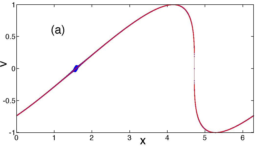
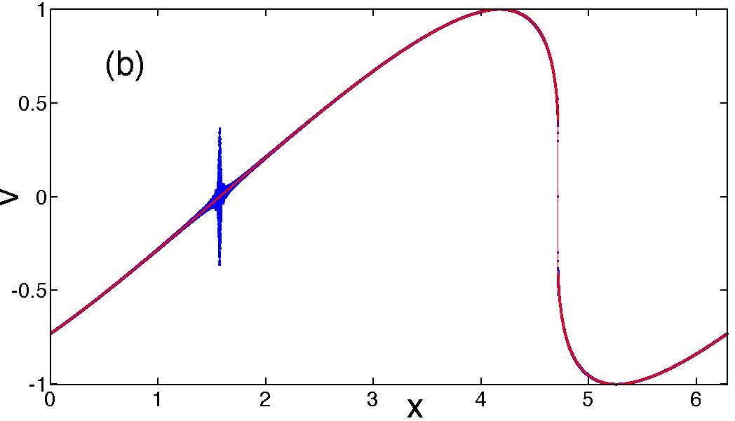
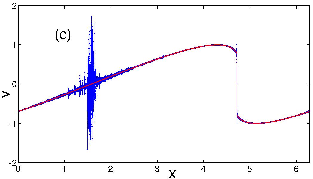
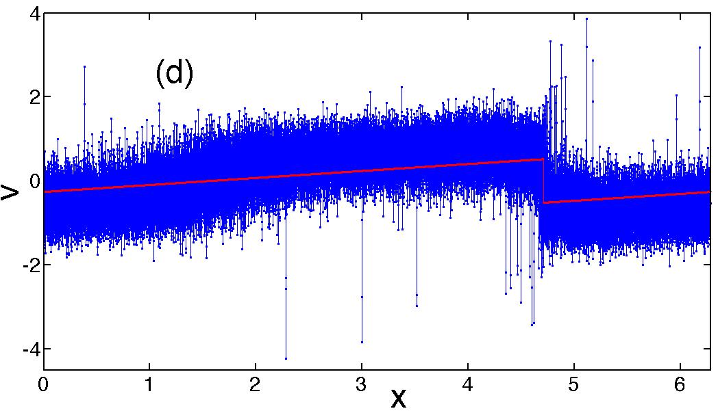
Figure 1: Solution of the Galerkin-truncated Burgers equation (4) $v$ (in blue) and the un-truncated Burgers equation (1) (entropy solution ) $u$ (in red) at different times for the initial condition $v_{0}=u_{0}=\sin(x+\phi)$ at different times $t\gtrsim t_{\star}$. At early times (a) $t=1.01$ the discrepancy between the two is small and localised around $x=x_{\rm tyger}$ where the velocity is dentical to that of the shock. This discrepancy, the tyger, grows (still remaining localised in space) in time as shown in (b) with $t=1.03$. At a later time (c) $t=1.15$, the symmetric, localised structure becomes asymmetric and starts spreading away from $x_{\rm tyger}$. Even at this time the truncated solution is able to duplicate the entropy solution at regions far away from $x_{\rm tyger}$ and in particular is able to capture the location and amplitude of the shock. At much later times, (d) $t=5.0$, the solution $v$ thermalises and becomes Gaussian, does not display the shock, and shows no similarity with the entropy solution $u$. This set of representative plots showing the birth and growth of tygers followed by the onset and eventual thermalisation of the solution were obtained from simulations with ${K_{\scriptscriptstyle\mathrm{G}}}=5000$ and $N=2^{16}$.

Thus, we begin with the one-dimensional inviscid Burgers equation

$$\frac{\partial u}{\partial t}+\frac{1}{2}\frac{\partial u^{2}}{\partial x}=0$$ (1)

augmented by the initial conditions $u_{0}(x)$ which are typically a combination of trigonometric functions containing a few Fourier modes. Without any loss in generality one can choose $u_{0}(x)=\sin(x+\phi)$; where $\phi$ is some random phase. Since we work in the space of $2\pi$ periodic solutions, we can expand the solution of Eq.(1) in a Fourier series

$$u(x)=\sum_{k=0,\pm 1,\pm 2\ldots}\mathrm{e}^{\mathrm{i}kx}\hat{u}_{k}.$$ (2)

This allows us to naturally define the Galerkin projector $\mathrm{P}_{\!\!\!{}_{K_{\scriptscriptstyle\mathrm{G}}}}$ as a low-pass filter which sets all modes with Fourier wavenumbers $|k|>{K_{\scriptscriptstyle\mathrm{G}}}$, where ${K_{\scriptscriptstyle\mathrm{G}}}$ is a positive (large) integer, to zero via

$$\mathrm{P}_{\!\!\!{}_{K_{\scriptscriptstyle\mathrm{G}}}}u(x)=\sum_{|k|\leq{K_{\scriptscriptstyle\mathrm{G}}}}\mathrm{e}^{\mathrm{i}kx}\hat{u}_{k}.$$ (3)

These definitions allow us to write the Galerkin-truncated inviscid Burgers equation as

$$\frac{\partial v}{\partial t}+\mathrm{P}_{\!\!\!{}_{K_{\scriptscriptstyle\mathrm{G}}}}\frac{1}{2}\frac{\partial v^{2}}{\partial x}=0;$$ (4)

the initial conditions $v_{0}=\mathrm{P}_{\!\!\!{}_{K_{\scriptscriptstyle\mathrm{G}}}}u_{0}$ are similarly projected onto the subspace spanned by ${K_{\scriptscriptstyle\mathrm{G}}}$. This defines the Galerkin-truncated velocity $v$ of the Burgers equation. For the three-dimensional Euler equations, the same definition follows mutatis mutandis.

The inviscid Burgers equation  (1) conserves all moments of the velocity field; by contrast the Galerkin-truncated version of it  (4) retains only the first three moments of $v$, and in particular the energy. Numerically, however, the dynamics of the Galerkin-truncated Burgers captures rather well the blowing up (with smooth initial conditions) of the gradient of the solution to the inviscid Burgers partial differential equation in a finite time $t_{\star}$. Indeed the cubic-root singularity (preshock), at $t_{\star}=\frac{1}{\rm{max}[\partial_{x}u]}\approx\frac{1}{\rm{max}[\partial_{x}v]}$, in $u$ (1) is also seen in the solution $v$ of the Galerkin-truncated equation ray11 ; burgreview1 ; burgreview2 ; fournierfrisch . Theoretically, the solution to  (1) for times greater than $t_{\star}$ is obtained by adding a tiny viscous dissipation term $\nu\frac{\partial^{2}u}{\partial x^{2}}$, with $\nu\to 0$ (the inviscid limit), which yield, depending on the initial conditions, finitely many shocks for times $t>t_{\star}$ hopf . This generalised solution, which converges weakly to the inviscid Burgers equation (1), is characterised by the dissipative anomaly: energy dissipation $\epsilon$ remains finite (with an associated non-conservation of the total energy) as $\nu\to 0$. This is very different to the dynamics of the Galerkin-truncated equation (4) whose solution $v$ stays smooth, conserves energy for all times $t>t_{\star}$ and later thermalises.

III Simulation Details

We perform extensive and state-of-the art simulations to obtain solutions for $u$ (1) and $v$ (4) for all times.

The true or entropy solution to the inviscid Burgers equation  (1) is obtained by the method of Fast Legendre Transform, which takes the limit $\nu\to 0$, developed by Noullez and Vergassola noullez (see also Refs. bec00 ; mitra05 ). This method takes advantage of the fact burgreview1 ; burgreview2 that the velocity potential $\psi$ defined via $u=-\frac{\partial\psi}{\partial x}$ is constrained by the maximum principle such that

$$\psi(x,s)=\max_{y}\left[\psi(y,t)-\frac{(x-y)^{2}}{2\,(s-t)}\right];$$ (5)

where $s>t$. We typically use the number of collocation points $N=2^{14}$ or $2^{16}$ and choose a time step $\delta t$ large enough for a Lagrangian particle to move by a distance equal to or larger than the grid spacing $\delta x$, and smaller than all other time scales associated with the dynamics.

We, of course, use a different strategy to solve the Galerkin-truncated equation (4). We use a pseudo-spectral method dns coupled to a fourth-order Runge–Kutta time marching with the total collocation points $N=2^{14}$ or $2^{16}$ as before. We use different values of ${K_{\scriptscriptstyle\mathrm{G}}}$, ranging from 700 to 20,000. Our time step $\delta t$ varied from $10^{-4}$ for ${K_{\scriptscriptstyle\mathrm{G}}}\leq 5,000$ to $10^{-5}$ for ${K_{\scriptscriptstyle\mathrm{G}}}>5,000$. Full dealiasing was ensured in this problem via ${K_{\scriptscriptstyle\mathrm{G}}}$.

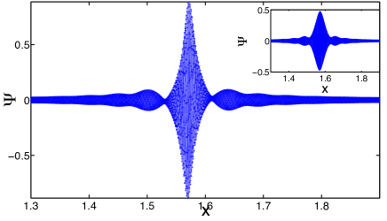
Figure 2: A representative zoomed-in plot of the discrepancy $\Psi=v-u$, around $x_{\rm tyger}$ for ${K_{\scriptscriptstyle\mathrm{G}}}=4000$ just when the bulge becomes asymmetric $t=T_{c}$ and (inset) when it is still symmetric $t<T_{c}$. The tyger, apart from being localised, is monochromatic with a single wavenumber ${K_{\scriptscriptstyle\mathrm{G}}}$ before $T_{c}$ (inset) ray11 ; for $t\geq T_{c}$, other harmonics smaller than ${K_{\scriptscriptstyle\mathrm{G}}}$ are generated as well.

IV Results

IV.1 Tygers and Thermalisation

We begin by performing direct numerical simulations of equations (1) and (4), without any loss of generality ray11 ; ray-review , with initial conditions $u_{0}(x)=v_{0}(x)=\sin(x+\phi)$, where $\phi=0.7$ is a phase which shifts the location of the cubic singularity away from $x=\pi$. For such an initial condition, it is easy to show that $t_{\star}=1.0$ burgreview1 ; burgreview2 . The time evolution of the solution to the untruncated Burgers equation $u(x)$ and the truncated Burgers equation $v(x)$ are shown in Fig. 1. For times $t\lesssim t_{\star}=1.0$, $v=u$ $\forall x$ as shown before . At $t=t_{\star}$ (in this case $t_{\star}=1.0$) and thereafter the discrepancy between the entropic solution $u(x)$ (in red) and $v(x)$ (in blue) is large as seen in Fig. 1. At early times, $t\gtrsim t_{\star}$, this discrepancy is localised (Figs. 1a and 1b); at later times (Fig. 1c) the solution to the Galerkin truncated equation starts deviating strongly from the entropy solution till at very large times it thermalises and shows a white-noise behaviour markedly different from the saw-tooth entropic solution (Fig. 1d).

A useful framework to study the departure from the entropy solution to the thermalised solution is via the discrepancy $\Psi=v-u$. For $t\lesssim t_{\star}$, $\Psi=0$. However, as shown in Ref. ray11 , at $t=t_{\star}$, at points which have the same velocity as the shock(s), $\Psi\neq 0$ and a symmetric, localised, monochromatic bulge, called tyger by Ray, et al. ray11 , forms as shown in Fig. 2 (inset). As time evolves, this bulge grows in amplitude $\alpha$ and width $\beta$, becomes asymmetric (Fig. 2, at $t=1.07$), collapses, delocalises, and eventually invades the whole $2\pi$-domain (Figs. 1c and 1d).

We now know that finite-dimensional equations of hydrodynamics thermalise through wave-particle resonances. Such resonances at early times manifest themselves as localised structures at the instant $t_{\rm G}\lesssim t_{\star}$, when complex singularities are within one Galerkin wavelength $\lambda_{\rm G}=\frac{2\pi}{{K_{\scriptscriptstyle\mathrm{G}}}}$ of the real domain. This was shown to be true for both the compressible Burgers equation as well as the incompressible Euler equations ray11 ; ray-review . Indeed the scaling properties of the early tygers at $t=t_{\star}$ were derived in Ref. ray11 and in particular the amplitudes and widths were shown to scale as $\alpha\sim{K_{\scriptscriptstyle\mathrm{G}}}^{-2/3}$ and $\beta\sim{K_{\scriptscriptstyle\mathrm{G}}}^{-1/3}$, respectively. Finally it was shown through detailed numerical simulations that in a short time these monochromatic, with wavelength $\lambda_{\rm G}$, localised, symmetric tygers become skewed, collapse, and spread throughout $0\leq x\leq 2\pi$, generate other harmonics, and eventually result in a thermalised solution with energy equipartition $E(k)\sim k^{0}$. However the critical question of the time $T_{c}$ when thermalisation is triggered has been left unanswered in previous studies. In this work we obtain a precise estimate of $T_{c}$ as a function of ${K_{\scriptscriptstyle\mathrm{G}}}$ and substantiate our theoretical prediction through detailed numerical simulations.

IV.2 Onset time

Before we present our theoretical prediction for $T_{c}$, it is important at this stage to provide a more precise definition of this time.

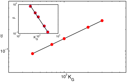
Figure 3: (Log-log plots of the tyger amplitudes $\alpha$ and widths $\beta$ (inset), shown by large red dots, versus ${K_{\scriptscriptstyle\mathrm{G}}}$ at a fixed time $t=1.05$ from our simulations. The thick black line, both in the inset and the main figure, correspond to the theoretical prediction of $\beta\sim{K_{\scriptscriptstyle\mathrm{G}}}^{-1}$ and $\alpha\sim{K_{\scriptscriptstyle\mathrm{G}}}^{1/2}$, respectively. We find remarkable agreement between our analytical prediction and numerical data. We note that for reasons outlined in the text, we show data for values of ${K_{\scriptscriptstyle\mathrm{G}}}$ for which $T_{c}>1.05$.

Detailed numerical simulation show (Figs. 1 and 2 as well as in Ref. ray11 ) that in the early stages $t\gtrsim t_{\star}$ the discrepancy $\Psi$ is small and localised at $x=x_{\rm tyger}$, where $x_{\rm tyger}$ are points co-moving with the shock. With time this bulge becomes bigger (still symmetric and localised), narrower (see Fig. 2), and the associated Reynolds stresses start increasing. At a critical time, the Reynolds stress becomes large enough to make the bulge asymmetric. This leads to a collapse of the bulge, accompanied by a spatial spreading of the oscillations as well as the generation of different harmonics, and the triggering of thermalisation of the system. We define this critical time $T_{c}$ as the time for onset of thermalisation. We note that numerically $T_{c}$ is well-defined and easy to measure given that the asymmetry in the bulge $\Psi$ can be determined clearly from the difference in the position of the positive and negative peaks: This difference is zero for $t_{\star}\leq t\leq T_{c}$ and becomes non-zero for $t>T_{c}$.

Before we proceed further, it is important at this stage to define the nomenclature which we will use in obtaining our estimate for the time of the onset of thermalisation. As defined before, $t_{\star}=\frac{1}{\rm{max}[\partial_{x}u]}\approx\frac{1}{\rm{max}[\partial_{x}v]}$ is the time when the complex singularity reaches the real domain. It was shown that ray11 tygers are born at a slightly earlier time $T_{\rm b}$ such that $\tau_{b}\equiv t_{\star}-T_{\rm b}=\mathcal{O}\left({K_{\scriptscriptstyle\mathrm{G}}}^{-2/3}\right)$. We define a new time scale $\tau_{c}\equiv T_{c}-T_{\rm b}$ which gives the estimate of the time scale for the onset of thermalisation and we obtain theoretical results for the shifted time $\tau\equiv t-T_{\rm b}$. It should be noted that this is a natural choice for time since for $t<T_{\rm b}$ tygers do not exist. We will see below that $\tau_{c}$ indeed shows a power-law behaviour in ${K_{\scriptscriptstyle\mathrm{G}}}$ with a scaling form $\tau_{c}\sim{K_{\scriptscriptstyle\mathrm{G}}}^{\xi}$; in what follows we derive an explicit form for this new scaling exponent $\xi$ and verify our theoretical predictions with data from detailed numerical simulations.

	$\alpha\sim\tau^{\gamma_{\alpha}}{K_{\scriptscriptstyle\mathrm{G}}}^{\delta_{\alpha}}$		$\beta\sim\tau^{\gamma_{\beta}}{K_{\scriptscriptstyle\mathrm{G}}}^{\delta_{\beta}}$		$\tau_{c}\sim{K_{\scriptscriptstyle\mathrm{G}}}^{\xi}$
	$\gamma_{\alpha}$	$\delta_{\alpha}$	$\gamma_{\beta}$	$\delta_{\beta}$	$\xi$
Theory	7/4	1/2	-1	-1	$\xi=\frac{\delta_{\beta}-2\delta_{\alpha}}{2\gamma_{\alpha}-\gamma_{\beta}}$ = -4/9
Simulations	1.74 $\pm$ 0.04	0.50 $\pm$ 0.01	-0.97 $\pm$ 0.08	-1.01 $\pm$ 0.02	-0.46 $\pm$ 0.07

Table 1: A summary of the new scaling exponents that we derive in this work. We see an excellent agreement, within error-bars, between our theoretical prediction and the exponents obtained, independently, from direct numerical simulations.

We now turn our attention to the amplitude $\alpha$ and width $\beta$ of the tyger. Let the widths and amplitudes assume the scaling form $\beta\sim\tau^{\gamma_{\beta}}{K_{\scriptscriptstyle\mathrm{G}}}^{\delta_{\beta}}$ and $\alpha\sim\tau^{\gamma_{\alpha}}{K_{\scriptscriptstyle\mathrm{G}}}^{\delta_{\alpha}}$, respectively. It is important to note that the scaling ansätz introduce here for the widths and amplitudes of the bulge (tyger) at any time $\tau\equiv t-T_{b}$ is consistent with the result introduced in the previous section (and proved in ray11 ), namely the width and amplitude of the tyger at $t_{\star}$. This is because at $t=t_{\star}$, $\tau=\tau_{b}\sim{K_{\scriptscriptstyle\mathrm{G}}}^{-2/3}$ (see ray11 ) and thence the scaling relation of the previous section follows from this ansätz. This is an important check of self-consistency of the theory. The asymmetry in the bulge occurs when the gradient of the Reynolds stresses become order one at time $\tau_{c}$. The Reynolds stress is defined as $\overline{\Psi^{2}}$, where the overline indicates the typical, mesoscopic average (spatial) ($\alpha$) over lengthscale larger than the Galerkin wavelength but smaller than other macroscopic scales in the problem; thence, dimensionally, the gradient of the Reynolds stress, namely $\frac{\alpha^{2}}{\beta}$, follows, since the relevant length scale over which this gradient should be taken $\sim\beta$. By using the assumed scaling form for $\alpha$ and $\beta$ one obtains the scaling form for the time of the onset of thermalisation as

$$\tau_{c}\sim{K_{\scriptscriptstyle\mathrm{G}}}^{\xi}\sim{K_{\scriptscriptstyle\mathrm{G}}}^{\frac{\delta_{\beta}-2\delta_{\alpha}}{2\gamma_{\alpha}-\gamma_{\beta}}}.$$ (6)

We thus obtain the first theoretical estimate for the onset time of thermalisation in a truncated equation of idealised hydrodynamics and obtain a new scaling exponent for the same, namely,

$$\xi=\frac{\delta_{\beta}-2\delta_{\alpha}}{2\gamma_{\alpha}-\gamma_{\beta}}.$$ (7)

It now behooves us to determine, self-consistently, the exponents $\gamma_{\alpha}$, $\gamma_{\beta}$, $\delta_{\alpha}$, and $\delta_{\beta}$ and verify our predictions from detailed numerical simulations.

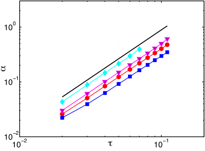
Figure 4: Log-log plots of the tyger amplitudes $\alpha$, for various values of the truncation wavenumber ${K_{\scriptscriptstyle\mathrm{G}}}$, as a function of the shifted time $\tau$. The different set of symbols correspond to different values of ${K_{\scriptscriptstyle\mathrm{G}}}$, namely, blue filled squares for ${K_{\scriptscriptstyle\mathrm{G}}}=400$; big red dots for ${K_{\scriptscriptstyle\mathrm{G}}}=700$; filled pink triangles for ${K_{\scriptscriptstyle\mathrm{G}}}=1000$; and filled cyan diamond for ${K_{\scriptscriptstyle\mathrm{G}}}=2000$. For each value of ${K_{\scriptscriptstyle\mathrm{G}}}$, our theoretical prediction $\alpha\sim\tau^{7/4}$, shown via thick black lines, seems to be in excellent agreement with the numerical data.

As we know that the Galerkin-truncated Burgers equation conserves energy for all time while displaying spatio-temporal chaotic behaviour at time $t\gg t_{\star}$. This is unlike the case of the entropy or untruncated solution $u$ of (1) which dissipate energy $\epsilon_{\rm shock}$ through the shock for time $t\geq t_{\star}$. Therefore for the truncated equation to conserve energy, $\epsilon_{\rm shock}$ gets transferred to the tygers via a resonant-wave-particle mechanism. Given that the estimate of energy contained in the tyger is $\alpha^{2}\beta$, this implies that for different values of ${K_{\scriptscriptstyle\mathrm{G}}}$, the energy content of the tyger must be the same. This immediately suggests that for any finite $\tau$, the integral $\int_{0}^{\tau}\alpha^{2}\beta dt$ is independent of ${K_{\scriptscriptstyle\mathrm{G}}}$. By using this argument we obtain the relation

$$2\delta_{\alpha}+\delta_{\beta}=0.$$ (8)

Spatially the tygers are confined, due to resonance, to a region of width $w$. For the tyger to grow, coherently, in a time interval $\tau$, phase mixing constrains this region to be of an extent such that the velocity difference across $w$ is of the order of $\lambda_{G}/\tau$. Since $\lambda_{G}=2\pi/{K_{\scriptscriptstyle\mathrm{G}}}$ and the velocity difference across $w$ is proportional to $w$, this implies that

$$\beta\sim\frac{1}{\tau{K_{\scriptscriptstyle\mathrm{G}}}}$$ (9)

yielding the exponents $\gamma_{\beta}=\delta_{\beta}=-1$. Furthermore, from  (8), we obtain $\delta_{\alpha}=1/2$.

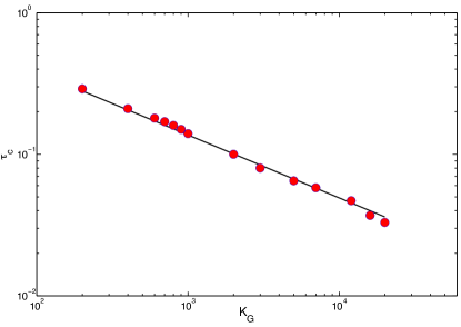
Figure 5: Log-log plot of the onset time $\tau_{c}$ for thermalisation versus ${K_{\scriptscriptstyle\mathrm{G}}}$. The data from our simulations is shown by big red dots; the thick black line connecting the data points is the theoretical prediction $\tau_{c}\sim{K_{\scriptscriptstyle\mathrm{G}}}^{-4/9}$. Note the excellent agreement between our data and the theoretical prediction for smaller values of ${K_{\scriptscriptstyle\mathrm{G}}}$ as compared to the larger values of ${K_{\scriptscriptstyle\mathrm{G}}}$. Possible reasons for this discrepancy is discussed in the text.

In Fig. 3 we show plots of $\alpha$ and $\beta$ (inset) at a given time $t=1.05$ as a function of ${K_{\scriptscriptstyle\mathrm{G}}}$. The thick black line connecting our data from numerical simulations (shown as large red dots) correspond to the theoretical prediction of $\delta_{\alpha}\sim{K_{\scriptscriptstyle\mathrm{G}}}^{1/2}$ and $\delta_{\beta}\sim 1/{K_{\scriptscriptstyle\mathrm{G}}}$. The figure shows not only a clear scaling, for both, but also an excellent agreement of our numerical data with our theoretical predictions as well as validating our assumptions in arriving at our analytical results. We note that the range of ${K_{\scriptscriptstyle\mathrm{G}}}$ shown in this figure does not extend all the way to our full range (e.g., see Fig. 5). This is because at the time $t=1.05$, for which the data is shown, solutions to the truncated equation with ${K_{\scriptscriptstyle\mathrm{G}}}$ greater than 3000 have already thermalised (see Fig. 5); hence the tygers have already collapsed for such wavenumbers at $t=1.05$ and thus the measurement of their amplitudes and widths do not make sense. Our choice of $t=1.05$ is motivated by having a time reasonably larger than $t_{\star}$ for which we still have a large range in ${K_{\scriptscriptstyle\mathrm{G}}}$ to clearly illustrate the theoretically predicted scaling behaviour.

Finally let us determine $\gamma_{\alpha}$. Let us consider $t=t_{\star}$, which, as we have noted before and proved in Ref. ray11 , implies $\tau\sim{K_{\scriptscriptstyle\mathrm{G}}}^{-2/3}$. At time $t_{\star}$, the untruncated equation shows a cubic root singularity. This implies, that because of Galerkin truncation the energy lost in the shock – and hence gained as $\alpha^{2}\beta$ in the tyger – is estimated as $\int_{0}^{\lambda_{G}}x^{2/3}dx\sim{K_{\scriptscriptstyle\mathrm{G}}}^{-5/3}$. Setting $\tau={K_{\scriptscriptstyle\mathrm{G}}}^{-2/3}$, and using our previously obtained estimate $\gamma_{\beta}=\delta_{\beta}=-1$ and $\delta_{\alpha}=1/2$, this suggests that

$${K_{\scriptscriptstyle\mathrm{G}}}^{\frac{-4\gamma_{\alpha}+2}{3}}\sim{K_{\scriptscriptstyle\mathrm{G}}}^{-5/3}.$$ (10)

Hence we obtain $\gamma_{\alpha}=7/4$.

From our simulations we calculate $\alpha$ for different values of ${K_{\scriptscriptstyle\mathrm{G}}}$ and show plots $\alpha$ vs $\tau$ for representative values of ${K_{\scriptscriptstyle\mathrm{G}}}$ in Fig. 4. The thick black line, which is $\propto\tau^{7/4}$ is our theoretical prediction that for a given value of ${K_{\scriptscriptstyle\mathrm{G}}}$, the amplitude of the tyger (upto the time of collapse) scales as $\alpha\sim\tau^{7/4}$. As in Fig. 3, we find excellent agreement between data obtained from our simulations with the theoretical prediction.

Having obtained theoretically, and validated through simulations (Figs.  3 and 4), the values of the scaling exponents of the amplitude and width of the tygers before they collapse, let us once again return to the issue of the scaling of the onset time of thermalisation $\tau_{c}$. We had obtained before the scaling form of $\tau_{c}$ in Eq. 6. We now use the values of the various exponents obtained thence to show, from Eq. 7, that $\xi=-4/9$, implying that thermalisation is triggered at a time

$$\tau_{c}\sim{K_{\scriptscriptstyle\mathrm{G}}}^{-4/9}.$$ (11)

A summary of all these exponents is given in Table 1.

We now turn to our numerical simulations and obtain, for different values of ${K_{\scriptscriptstyle\mathrm{G}}}$, the time of collapse $\tau_{c}$. In our numerical simulations we actually measure $\tau_{c}$ by using $t_{\star}$ (instead of $T_{b}$) as the reference time, i.e., $\tau_{c}\equiv T_{c}-t_{\star}$. The reason for this is because for the simulations we wanted a unique reference time $t_{\star}$ which is independent of ${K_{\scriptscriptstyle\mathrm{G}}}$ (unlike $T_{b}$). This also reduces significantly any measurement error in estimating $T_{b}$. Such a definition of $\tau_{c}$, for our numerical simulations, is justified because for the values of ${K_{\scriptscriptstyle\mathrm{G}}}$ used in our simulations, $T_{b}$ and $t_{\star}$ are extremely close to each other ray11 and there is an order of magnitude separation between the time scales $\tau_{b}$ and $\tau_{c}$.

In Fig. 5, we show (red dots) the data obtained from our simulations. The thick black line corresponds to the theoretical prediction (11). We find excellent agreement between our analytical prediction and the data obtained from simulations. Despite this confirmation of our theoretical predictions, it is important to note that at extremely large values of ${K_{\scriptscriptstyle\mathrm{G}}}$ we see a noticeable discrepancy between the theoretical result and our data. The reasons for this are two-fold: Firstly, as ${K_{\scriptscriptstyle\mathrm{G}}}$ becomes larger and larger, $\tau_{c}$ become smaller and smaller. Hence a very accurate measurement of $\tau_{c}$, numerically, becomes harder because the relative error between the temporal resolution of our simulations and $\tau_{c}$ become larger. A second reason for this is that numerically, for reasons mentioned before, we measure $\tau_{c}$ relative to $t_{\star}$ and not $T_{b}$. Hence for large ${K_{\scriptscriptstyle\mathrm{G}}}$ when $\tau_{c}$ becomes smaller, our neglecting of $\tau_{b}$ (although there is an order of magnitude scale separation between $\tau_{c}$ and $\tau_{b}$) probably starts yielding a correction which is less neglible.

V Conclusions

In this paper we provide the first prediction, analytically and validated by numerically simulations, of the time when thermalisation is triggered in finite-dimensional inviscid equations of hydrodynamics and hence solves a very important problem in the interface of turbulence and statistical mechanics. We show that, through the Galerkin-truncated Burgers model, thermalisation is triggered on a time scale which decays as a power-law in ${K_{\scriptscriptstyle\mathrm{G}}}$ with an exponent which has been derived analytically by us and verified through numerical simulations.

Our results throw up important implications beyond the obvious realms of non-equilibrium statistical physics. This has to do with using numerical simulations for tracing complex singularities, in ideal equations of hydrodynamics, by using the method of the analyticity strip frisch83 . In recent years (we refer the reader to Ref. brachet for the most recent results and to Ref. blow-up for a recent review of results on finite-time blow-ups via numerical simulations), with the advance of computing power, the search for evidence for or against finite-time blow-up of the three-dimensional Euler equations through numerical simulations have gained ground. As shown by Bustamante and Brachet brachet , the temporal measurement of the distance, to the real domain, of the nearest singularity, is limited not only by computing power but also by the onset of thermalisation. Hence an estimate of the time when thermalisation sets in will be have an important bearing on interpreting the accuracy of measurements of complex singularities in time from spectral, and hence Galerkin-truncated, simulations of the Euler equations. We note in passing that the limitation in extrapolating in time the temporal evolution of the width of the analyticity strip has been noted, amongst others, in Ref. brachet .

There are of course several important questions which still remain unanswered. Foremost amongst them is the need to see, numerically, if a similar scaling argument holds for the incompressible three-dimensional Euler equation. This is a massively challenging task even with the modern day computers. Secondly the onset of thermalisation is necessarily accompanied by the generation of Fourier harmonics other than ${K_{\scriptscriptstyle\mathrm{G}}}$ which eventually lead to a white noise velocity field with a flat spectrum. The precise mechanism of this is yet to be understood in an analytical way. Furthermore, it has been observed (Fig. 2 as well as in Ref. ray11 ) that just prior to and after $\tau_{c}$, secondary bulges, reminiscent of the beating effect in acoustics, develop on either side of the tyger. A systematic theory which explains the full transition to thermalised states should capture this effect. These questions, and many more, are left for future work.

We thank Aritra Kundu for many useful discussions. Both authors acknowledge financial support from the AIRBUS Group Corporate Foundation Chair in Mathematics of Complex Systems established in ICTS-TIFR. SSR also acknowledges the support from DST (India) project ECR/2015/000361 and the Indo-French Center for Applied Mathematics (IFCAM). The direct numerical simulations were done on Mowgli at the ICTS-TIFR, Bangalore, India.

References

- (1) E. Hopf, Comm. Pure Appl. Math. 3, 201 (1950).
- (2) T. D. Lee, Q. J. Appl. Math. 10 (1952).
- (3) A.N. Kolmogorov, Dokl. Akad. Nauk SSSR 30, 301 (1941); A.N. Kolmogorov, Dokl. Akad. Nauk SSSR 31, 538 (1941).
- (4) R. Kraichnan, Phys. Fluids 10, 1417 (1967).
- (5) A. J. Majda and I. Timofeyev, Proc. Natl. Acad. Sci. 97 12413 (2000).
- (6) C. Cichowlas, P. Bonaïti, F. Debbash, and M. Brachet, Phys. Rev. Lett. 95, 264502 (2005).
- (7) R. H. Kraichnan and S. Chen, Physica D 37, 160 (1989).
- (8) U. Frisch, A. Pomyalov, I. Procaccia, and S. S. Ray, Phys. Rev. Lett. 108, 074501 (2012).
- (9) V. L’vov, A. Pomyalov and I. Procaccia, Phys. Rev. Lett. 89, 064501 (2002).
- (10) M. Buzzicotti, L. Biferale, U. Frisch, and S. S. Ray, Phys. Rev. E 93, 033109 (2016).
- (11) A. S. Lanotte, R. Benzi, S. K. Malapaka, F. Toschi, and L. Biferale, Phys. Rev. Lett. 115, 264502 (2015).
- (12) A. S. Lanotte, S. K. Malapaka, L. Biferale, Eur. Phys. J. E 39, 49 (2016).
- (13) M. Buzzicotti, A. Bhatnagar, L. Biferale, A. S. Lanotte, S. S. Ray, New J. of Phys. 18, 113047 (2016).
- (14) V. S. L’vov, S. V. Nazarenko, and O. Rudenko, Phys. Rev. B, 76, 024520 (2007).
- (15) C. Connaughton, Physica D, 238, 2282 (2009).
- (16) P. Feng, J. Zhang, S. Cao, S.V. Prants, Y. Liu, Commun. Nonlinear Sci. Numer. Simulat., 45, 104 (2017)
- (17) S. S. Ray, U. Frisch, S. Nazarenko, and T. Matsumoto, Phys. Rev. E 84, 16301 (2011).
- (18) S. S. Ray, in Persp. in Nonlinear Dynamics, Pramana - J. of Phys., 84, 395, (2015).
- (19) G. Krstulovic and M. Brachet, Phys. Rev. Lett., 106, 115303 (2011); G. Krstulovic and M. Brachet, Phys. Rev. E, 83, 066311 (2011); V Shukla, M Brachet, R Pandit, New Journal of Physics, 15, 113025 (2013).
- (20) G. Krstulovic, M. E. Brachet, and A. Pouquet, Phys. Rev. E, 84, 016410 (2011).
- (21) G. Krstulovic, P. D. Mininni, M. E. Brachet, and A. Pouquet, Phys. Rev. E,79, 056304 (2009).
- (22) U. Frisch, S. Kurien, R. Pandit, W. Pauls, S. S. Ray, A. Wirth, and J-Z Zhu, Phys. Rev. Lett. 101, 144501 (2008).
- (23) U. Frisch, S. S. Ray, G. Sahoo, D. Banerjee, and R. Pandit, Phys. Rev. Lett., 110, 64501 (2013).
- (24) D. Banerjee and S. S. Ray, Phys. Rev. E 90, 041001(R) (2014).
- (25) W. Dobler, N.E.L. Haugen, T.A. Yousef and A. Brandenburg, Phys. Rev. E, 68, 026304 (2003); Z.-S. She, G. Doolen, R.H. Kraichnan, and S.A. Orszag, Phys. Rev. Lett., 70, 3251 (1993); P.K. Yeung and Y. Zhou, Phys. Rev. E, 56, 1746 (1997); T. Gotoh, D. Fukayama, and T. Nakano, Phys. Fluids, 14, 1065 (2002); M.K. Verma and D.A. Donzis, J. Phys. A: Math. Theor., 40, 4401 (2007); P.D. Mininni, A. Alexakis, and A. Pouquet, Phys. Rev. E, 77, 036306 (2008). Y. Kaneda, et al., Phys. Fluids, 15, L21 (2003); T. Isihara, T. Gotoh, and Y. Kaneda Annu. Rev. Fluid Mech., 41, 165 (2009); S. Kurien, M.A. Taylor, and T. Matsumoto, Phys. Rev. E, 69, 066313 (2004); D.A. Donzis and K.R. Sreenivasan J. Fluid Mech., 657, 171 (2010); H.K. Pak, W.I. Goldburg, A. Sirivat, Fluid Dynamics Research, 8, 19 (1991); Z.-S. She and E. Jackson, Phys. Fluids A, 5, 1526 (1993); S.G. Saddoughi and S.V. Veeravalli, J. Fluid Mech., 268, 333 (1994); G. Falkovich, Phys. Fluids, 6, 1411 (1994); L. Sirovich, L. Smith, and V. Yakhot, Phys. Rev. Lett., 72, 344, (1994).
- (26) D. Gottlieb and S. A. Orszag, Numerical analysis of spectral methods: theory and applications, CBMS-NSF Regional Conference Series in Applied Mathematics 26, SIAM (1977).
- (27) U. Frisch, T. Matsumoto, and J. Bec, J. Stat. Phys. 113, 761 (2003); J. D. Gibbon, Physica D 237, 1894 (2008).
- (28) U. Frisch and J. Bec, Les Houches 2000: New Trends in Turbulence, Eds. : M. Lesieur, A. Yaglom and F. David, pp. 341-383, Springer EDP-Sciences, (2001).
- (29) J. Bec and K. Khanin, Phys. Rep. 447, 1-66, (2007).
- (30) P. D. Lax and C. D. Levermore, Proc. Natl. Acad. Sci. U.S.A. 76, 3602 (1979); J. Goodman and P. D. Lax, Commun. Pure Appl. Math. 41, 591 (1988); T. Y. Hou and P. D. Lax, Commun. Pure Appl. Math. 44, 1 (1991).
- (31) J.D. Fournier and U. Frisch, J. Méc. Théor. Appl. (Paris) 2, 699 (1983).
- (32) A. Noullez and M. Vergassola, J. Sci. Comp. 9, 259 (1994).
- (33) J. Bec, U. Frisch, and K. Khanin, J. Fluid Mech. 416, 239 (2000).
- (34) D. Mitra, J. Bec, R. Pandit, and U. Frisch, Phys. Rev. Lett. 94, 194501, (2005).
- (35) C. Sulem, P.-L. Sulem, H. Frisch, J. Comput. Phys. 50, 138 (1983).
- (36) M. D. Bustamante and M. Brachet, Phys. Rev. E 86, 066302 (2012).