LFADS - Latent Factor Analysis via Dynamical Systems
Abstract
Neuroscience is experiencing a data revolution in which many hundreds or thousands of neurons are recorded simultaneously. Currently, there is little consensus on how such data should be analyzed. Here we introduce LFADS (Latent Factor Analysis via Dynamical Systems), a method to infer latent dynamics from simultaneously recorded, single-trial, high-dimensional neural spiking data. LFADS is a sequential model based on a variational auto-encoder. By making a dynamical systems hypothesis regarding the generation of the observed data, LFADS reduces observed spiking to a set of low-dimensional temporal factors, per-trial initial conditions, and inferred inputs. We compare LFADS to existing methods on synthetic data and show that it significantly out-performs them in inferring neural firing rates and latent dynamics.
1 Introduction
Over the past two decades, the ability to record large numbers of neurons simultaneously has increased dramatically, primarily through the use of multi-unit electrode arrays and imaging technologies. The change from single-unit recordings to simultaneously recorded, high-dimensional data is exciting, but analyzing this data presents significant challenges. The traditional approach, necessitated by limited experimental observations, is to trial-average recorded spike trains from single neurons, perhaps with some temporal filtering, and then to construct peri-stimulus time histograms (PSTHs). Despite many attempts to make sense of high-dimensional neuroscience data, e.g. [5, 11, 13, 16, 20], the vast majority of experimental neuroscientists still use single-unit PSTHs in their analyses.
The most obvious challenge to advancing neural data analysis is that brains are immensely complex, and they solve multiple and varied problems ranging from vision to motor planning and navigation. Given the generality of the problems brains must solve, it is not surprising that no one-size-fits-all algorithm has yet materialized. Two ends of a spectrum for generic computation are feed-forward processing and sequential processing. In the feed-forward case, temporal dynamics play no role, and computation is purely input driven. In the sequential case, on the other hand, dynamics are paramount, and computation results from an autonomous nonlinear dynamical system starting from a specific initial condition and run for some period of time to produce “computational dynamics”.
Here we develop a deep learning architecture, called Latent Factor Analysis via Dynamical Systems (LFADS; “ell-fads”), which lies further towards the sequential end of this spectrum, while still allowing for external inputs and input driven dynamics. LFADS implements the hypothesis that a driven nonlinear dynamical system provides a reasonable model of many neural processes. The primary goal of LFADS is to infer smooth dynamics from recorded neural spike trains on a single-trial basis. In doing so, LFADS provides a number of other components that can aid in understanding the data better: a low-dimensional set of temporal factors that explain the observed spike trains, a recurrent network that produces the smoothed data and can be analyzed using techniques such as those found in [22], a set of initial conditions that can be used as a code for each trial (if the data is broken up into trials) and, finally, LFADS infers inputs. Inferring inputs is predicated on the idea that a dynamical system provides a notion of surprise, namely, if a powerful nonlinear dynamical system cannot generate the data then, necessarily, an external perturbation to the system must have occurred. Within the LFADS architecture, we learn this perturbation and identify it as an inferred input.
The ability of LFADS to infer input is an extremely useful feature for neuroscience research. Even extensive neural recordings cover only a tiny fraction of an animal’s neurons, which means that the recorded neurons receive input from other neurons that are not recorded. Unmeasured input introduces a major source of uncertainty into our understanding and modeling of neural circuits. Even in cases where we know that input is affecting a particular circuit, for example inputs due to sensory stimuli presented to the animal during the recording session, we typically do not know the form that this input takes. LFADS is designed to infer such inputs on the basis of the recorded data alone.
2 The LFADS Model
The LFADS model is an instantiation of a variational auto-encoder (VAE) [12, 19] extended to sequences, as in [9] or [14]. The VAE consists of two components, a decoder or generator and an encoder. The generator assumes that data, denoted by , arise from a random process that depends on a vector of stochastic latent variables , samples of which are drawn from a prior distribution . Simulated data points are then drawn from a conditional probability distribution, (we have suppressed notation reflecting the dependence on parameters of this and the other distributions we discuss).
The VAE encoder transforms actual data vectors, , into a conditional distribution over , . is a trainable approximation of the posterior distribution of the generator, . can also be thought of as an encoder from the data to a data-specific latent code , which can be decoded using the generator (decoder). Hence the autoencoder; the encoder maps the actual data to a latent stochastic “code", and the decoder maps the latent code back to an approximation of the data. Specifically, when the two parts of the VAE are combined, a particular data point is selected and an associated latent code, (we use to denote a sample of the stochastic variable ) is drawn from . A data sample is then drawn from , on the basis of the sampled latent variable. If the VAE has been constructed properly, should resemble the original data point .
The loss function that is minimized to construct the VAE involves minimizing the Kullbach-Liebler divergence between the encoding distribution and the prior distribution of the generator, , over all data points. Thus, if training is successful, these two distributions should converge and, in the end, statistically accurate simulations of the data can be generated by running the generator model alone.
We now translate this general description of the VAE into the specific LFADS implementation. Borrowing notation from [9], we denote an affine transformation from a variable to a variable as , we use to represent vector concatenation, and we denote a temporal update of a recurrent neural network receiving an input as .
2.1 LFADS Generator
The neural data we consider, , consists of spike trains from recorded neurons. Each instance of a vector is referred to as a trial, and trials may be grouped by experimental conditions, such as stimulus or response types. The data may also include an additional set of observed variables, , that may refer to stimuli being presented or other experimental features of relevance. Unlike , the data described by is not itself being modeled, but it may provide important information relevant to the modeling of . This introduces a slight complication: we must distinguish between the complete data set, and the part of the data set being modeled, . The conditional distribution of the generator, , is only over , whereas the approximate posterior distribution, , depends on both types of data.
LFADS assumes that the observed spikes described by are samples from a Poisson process with underlying rates . Based on the dynamical systems hypothesis outlined in the Introduction, the goal of LFADS is to infer a reduced set of latent dynamic variables, , from which the firing rates can be constructed. The rates are determined from the factors by an affine transformation followed by an exponential nonlinearity, . The choice of a low-d representation for the factors is based on the observation that the intrinsic dimensionality of neural recordings tends to be far lower than the number of neurons recorded, e.g. [5, 11, 16], and see [6] for a more complete discussion.
The factors are generated by a recurrent nonlinear neural network and are characterized by an affine transformation of its state vector, . Running the network requires an initial condition , which is drawn from a prior distribution . Thus, is part of the stochastic latent variable discussed above.
There are different options for sources of input to the recurrent generator network, First, as in some of the examples to follow, the network may receive no input at all. Second, it may receive the information contained in the non-modeled part of the data, , in the form of a network input. We discuss this option in the Discussion, but we do not implement it here. Instead, as a third option, we introduce an inferred input . When an inferred input is included, the stochastic latent variable is expanded to include it, . At each time step, is drawn from a prior distribution .
The LFADS generator with inferred input is thus described by the following procedure and equations. First an initial condition for the generator is sampled from the prior
| (1) |
At each time step , an inferred input, , is sampled from its prior and fed into the network, and the network is evolved forward in time,
| (2) | ||||
| (3) | ||||
| (4) | ||||
| (5) | ||||
| (6) |
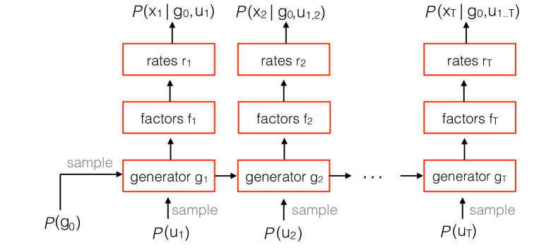
Here “Poisson" indicates that each component of the spike vector is generated by an independent Poisson process at a rate given by the corresponding component of the rate vector . The priors for both and , , are diagonal Gaussian distributions with zero mean and a fixed chosen variance (see Appendix). We chose the GRU [3] as our recurrent function for all the networks we use (defined in the Appendix). We have not included the observed data in the generator model defined above, but this can be done simply by including as an additional input to the recurrent network in equation 3. Note that doing so will make the generation process necessarily dependent on including an observed input. The generator model is illustrated in Fig. 1. This diagram and the above equations implement the conditional distribution of the VAE decoder.
2.2 LFADS Encoder
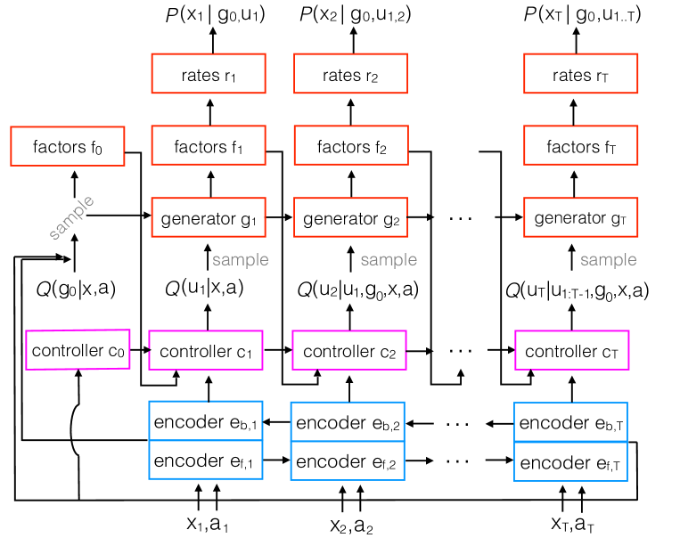
The approximate posterior distribution for LFADS is the product of two conditional distributions, one for and one for . Both of these distributions are diagonal Gaussians with means and variances determined by the outputs of the encoder or controller RNNs (see Fig. 2 and below). We begin by describing the network that defines . Its mean and variance are given in terms of a variable by
| (7) | ||||
| (8) |
is obtained by running a recurrent network both forward (from to ) and backward (from to ) in time,
| (9) | ||||
| (10) |
with and learnable parameters. Once this is done, is the concatenation
| (11) |
Running the encoding network both forward and backward in time allows to reflect the entire time history of the data and .
The approximate posterior distribution for is defined in a more complex way that involves both an encoder network and another RNN called the controller. The encoder network with state variables and is described by equations identical to 9 and 10 (although with different trainable network parameters), and these serve to define the time-dependent variable
| (12) |
Rather than feeding directly into a Gaussian distribution, this variable is passed through the controller RNN, which also receives the latent dynamic factor, as input,
| (13) |
Thus, the controller is privy to the information about and encoded in the variable , and it receives information about what the generator network is doing through the latent dynamic factor . It is necessary for the controller to receive the factors so that it can correctly decide when to intervene in the generation process. Because depends on both and , these stochastic variables are included in the conditional dependence of the approximate posterior distribution . The initial state of the controller network, , is defined deterministically, rather than drawn from a distribution, by the affine transformation
| (14) |
in this expression is the same variable that determines the mean and the variance of the distribution from which is drawn, as defined by equations 9-11.
Finally, the inferred input, , at each time, is a stochastic variable drawn from a diagonal Gaussian distribution with mean and log-variance given by an affine transformation of the controller network state, ,
| (15) |
with
| (16) | ||||
| (17) |
We control the information flow out of the controller and into the generator by applying a regularizer on (a KL divergence term, described below and also in the Appendix), and also by explicitly limiting the dimensionality of , the latter of which is controlled by a hyper parameter.
2.3 The full LFADS inference model
The full LFADS model (Fig. 2) is run in the following way. First, a data trial is chosen, the encoders are run, and an initial condition is sampled from the approximate posterior . An initial condition for the controller is also sampled (equation 14). Then, for each time step from 1 to , the generator is updated, as well as the factors and rates, according to
| (18) | ||||
| (19) | ||||
| (20) | ||||
| (21) | ||||
| (22) | ||||
| (23) | ||||
| (24) | ||||
| (25) |
After training, the full model can be run, starting with any single trial or a set of trials corresponding to a particular experimental condition to determine the associated dynamic factors, firing rates and inferred inputs for that trial or condition. This is done by averaging over several runs to marginalize over the stochastic variables and .
2.4 The loss function
To optimize our model, we would like to maximize the log likelihood of the data, , marginalizing over all latent variables. For reasons of intractability, the VAE framework is based on maximizing a lower bound, , on the marginal data log-likelihood,
| (26) |
is the log-likelihood of the reconstruction of the data, given the inferred firing rates, and is a non-negative penalty that restricts the approximate posterior distribution for deviating too far from the prior distribution. These are defined as
| (27) | ||||
| (28) |
where the brackets denote marginalizations over the subscripted variables. Evaluating the KL terms can be done analytically for the Gaussian distributions we use; the formulae are found in Appendix B of [12]. We minimize the negative bound, , using the reparameterization trick to back-propagate low-variance, unbiased gradient estimates. These gradients are used to train the system in an end-to-end fashion, as is typically done in deterministic settings.
3 Relation to Previous Work
Recurrent neural networks have been used extensively to model neuroscientific data (e.g. [21] [16], [2], [23], [18]), but the networks in these studies were all trained in a deterministic setting. An important recent development in deep learning has been the advent of the variational auto-encoder [12] [19], which combines a probabilistic framework with the power and ease of optimization of deep learning methods. VAEs have since been generalized to the recurrent setting, for example with variational recurrent networks [4], deep Kalman filters [14], and the RNN DRAW network [9].
There is also a line of research applying probabilistic sequential graphical models to neural data. Recent examples include PLDS [15], switching LDS [17], GCLDS [8], and PfLDS [7]. These models employ a linear Gaussian dynamical system state model with a generalized linear model (GLM) for the emissions distribution, typically using a Poisson process. In the case of the switching LDS, the generator includes a discrete variable that allows the model to switch between linear dynamics. GCLDS employs a generalized count distribution for the emissions distribution. Finally, in the case of PfLDS, a nonlinear feed-forward function (neural network) is inserted between the LDS and the GLM.
Gaussian process models have also been explored. GPFA [24] uses Gaussian processes (GPs) to infer a time constant with which to smooth neural data and has seen widespread use in experimental laboratories. More recently, the authors of [26] have used a variational approach (vLGP) to learn a GP that then passes through a nonlinear feed-forward function to extract the single-trial dynamics underlying neural spiking data.
The authors of [14] have defined a very general nonlinear variational sequential model, which they call the Deep Kalman Filter (DKF). The authors then apply a DKF to a synthetic “healing MNIST” task. Due to the generality of the DKF equations, LFADS is likely one of many possible instantiations of a DKF applied to neural data (in the same sense that a convolutional network architecture applied to images is also a feed-forward network, for example).
Like a Kalman filter, LFADS decomposes data into a set of inferred dynamics and a set of innovation-like quantities that help explain the observed data when the state model cannot. Recasting our work in the language of Kalman filters, our nonlinear generator is analogous to the linear state estimator in a Kalman filter, and we can think of the inferred inputs in LFADS as innovations in the Kalman filter language. However, an “LFADS innovation” is not strictly defined as an error between the measurement and the readout of the state estimate. Rather, the LFADS innovation may depend on the observed data and the generation process in extremely complex ways.
4 Results
We compared the performance of LFADS to three existing methods that estimate latent state from neural data: GPFA [24], vLGP [26], and PfLDS [7]. To test LFADS and to compare its performance with other approaches, we generated synthetic stochastic spike trains from two different deterministic nonlinear systems. The first is the standard Lorenz system. The second is a recurrent nonlinear neural network that we call the data RNN (to distinguish it from the RNNs within LFADS). For these two systems, we compared LFADS without any inferred input (because none is needed) with other methods. We also added an input to the data RNN to highlight the inferred input feature of LFADS. As shown below, in the first two cases, LFADS outperforms the other methods, and in the third case, LFADS is able to infer the timing of the actual input quite reliably.
4.1 Lorenz system
The Lorenz system is a set of nonlinear equations for three dynamic variables. Its limited dimensionality allows its entire state space to be visualized. The evolution of the system’s state is governed as follows
| (29) | ||||
| (30) | ||||
| (31) |
We used standard parameter values , , and , and used Euler integration with . As in [26], we simulated a population of neurons with firing rates given by linear readouts of the Lorenz variables using random weights, followed by an exponential nonlinearity. Spikes from these firing rates were then generated by a Poisson process. We then tested the ability of each method to infer the latent dynamics of the Lorenz system (i.e., the values of the three dynamic variables) from the spiking activity alone.
Our synthetic dataset consisted of 65 conditions, with 20 trials per condition. Each condition was obtained by starting the Lorenz system with a random initial state vector and running it for 1s. Twenty different spike trains were then generated from the firing rates for each condition. Models were trained using 80% of the data (16 trials/condition) and evaluated using 20% of the data (4 trials/condition). Fig. 3 shows the Lorenz variables and spike times for an example trial. While this simulation is structurally quite similar to the Lorenz system used in [26], we purposefully chose parameters that made the dataset more challenging. Specifically, relative to [26], we limited the number of observations to 30 simulated neurons instead of 50, decreased the baseline firing rate from 15 spikes/sec to 5 spikes/sec, and sped up the dynamics by a factor of 4.


| Dim | vLGP | GPFA | PfLDS | LFADS |
|---|---|---|---|---|
| y1 | 0.477 | 0.713 | 0.784 | 0.826 |
| y2 | 0.377 | 0.725 | 0.732 | 0.900 |
| y3 | 0.015 | 0.325 | 0.368 | 0.821 |
Fig. 4 shows the Lorenz latent dynamics for an example trial and the latent dynamics inferred by each method (for LFADS, posterior means averaged over 128 samples of conditioned on the particular input sequence). For each method, the inferred latents linearly transformed to the actual latents to facilitate direct comparison. As shown, LFADS accurately recovered the latent dynamics underlying the observed spike trains, consistently outperforming the three other methods. We quantify this using , i.e., the fraction of the variance of the actual latent variables captured by the estimated latent values (Table 1).
4.2 Inferring the dynamics of a chaotic RNN
Next we tested the performance of each method at inferring the dynamics of a more complex nonlinear dynamical system, a fully recurrent neural network with strong coupling between the units. We generated a synthetic dataset from an -dimensional continuous time nonlinear, so-called, “vanilla" RNN,
| (32) |
This makes a compelling synthetic case study for our method because many recent studies of neuroscientific data have used vanilla RNNs as their modeling tool (e.g. [21] [16], [2], [23], [18]). It should be stressed that the vanilla RNN used as the data RNN here does not have the same functional form as the network generator used in the LFADS framework, which is a GRU (see Appendix). In this example, we set , but we include an input in the following section.
The elements of the matrix were drawn independently from a normal distribution with zero mean and variance . We set , which produces chaotic dynamics at a relatively slow timescale compared to (see [21] for more details). Specifically, we set , s and used Euler integration with s. Spikes were generated by a Poisson process with firing rates obtained by shifting and scaling to give rates lying between 0 and 30 spikes/s (Fig. 5).
Our dataset consisted of 400 conditions obtained by starting the data RNN at different initial states with elements drawn from a normal distribution with zero mean and unit variance. Firing rates were then generated by running the data RNN for 1 s, and 10 spiking trials were produced for each condition. Models were trained using 80% of the data (8 trials/condition) and evaluated using 20% of the data (2 trials/condition). Fig. 5 shows underlying firing rates and spiking activity for a single trial.
We used principal components analysis to determine the number of latent variables needed to describe the data. As expected, the state of the data RNN has lower dimension than its number of neurons, and 20 principal components are sufficient to capture of the variance of the system (Fig. 5). We therefore restricted the latent space to 20 dimensions for each of the models tested and, in the case of LFADS, set the number of temporal factors to 20 as well.

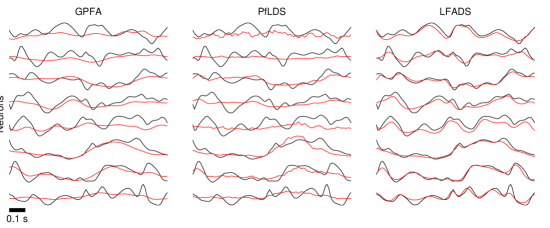
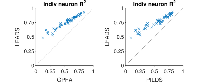
We tested the performance of the methods at extracting the underlying firing rates from the spike trains of the RNN dataset. We restricted this comparison to the three best-performing methods from the Lorenz comparison (GPFA, PfLDS and LFADS) because the vLGP results were noticeably worse in that case. An example of actual and inferred rates extracted by each model is shown in Fig. 6. As can be seen by eye, the LFADS results are closer to the actual underlying rates than for the other models. We summarize this again using values between the actual and inferred rates in Fig. 7.
4.3 Inferring inputs to a chaotic RNN
Finally, we tested the ability of LFADS to infer the input to a dynamical system, specifically the data RNN used in the previous section. In general, the problem of disambiguating dynamics from inputs is ill-posed, so we encouraged the dynamics to be as simple as possible by including an L2 regularizer in the LFADS network generator (see Appendix). We note that regularization is a standard technique that is nearly universally applied to neural network architectures. As shown below, adding a regularizer does not mean that the dynamics play no role. Rather it ensures that if a low-dimensional inferred input can aid in explaining the data, the optimization cost will be reduced by using it instead of building a more complex dynamics. By low-dimensional inferred inputs, we mean that the dimensionality of should be lower dimensional than the data we are attempting to model.
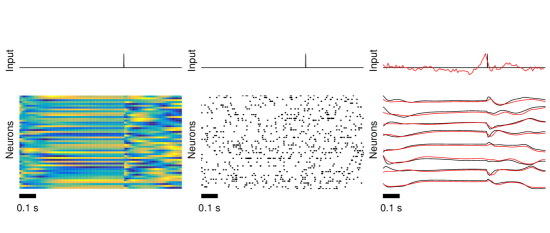
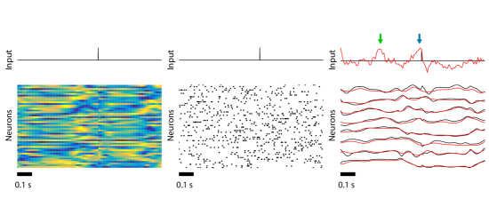
To introduce an input into the data RNN, the elements of were drawn independently from a normal distribution with zero mean and unit variance. During each trial, we perturbed the network by delivering a delta pulse of magnitude 50, , at a random time between 0.25s and 0.75s (the full trial length was 1s). This pulse affects the underlying rates produced by the data RNN, which modulates the spike generation process. To test the ability of the LFADS model to infer the timing of these input pulses, we included in the LFADS model an inferred input with dimensionality of 1. We explored two values of , 1.5 and 2.5. The lower value produces “gentler" chaotic activity in the data RNN than the higher value. Otherwise, the data for this example (Fig. 8 and Fig. 9) were generated as in the first data RNN example described above.
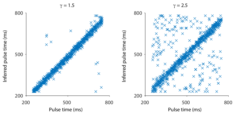
After training, which successfully inferred the firing rates (e.g. Figs. 8 and 9, right panels), we extracted inferred inputs from the LFADS model (eqn. 15) by running the system 512 times for each trial, and averaging, defining . To see how this was related to the actual input pulse, we determined the time at which reached its maximum value. The results are plotted in Fig. 10 and demonstrate that, for the vast majority of trials, LFADS inferred that there was an input near the time of the actual delta pulse.
LFADS did a better job of inferring the inputs in the case of simpler dynamics (i.e., , Fig. 8) than for more complex dynamics (, Fig. 9). This occurs for two reasons. First, in the case of , the complex dynamics reduces the magnitude of the perturbation caused by the input. Second, in the case, LFADS used the inferred input more actively to account for the non-input-driven dynamics as well as the input driven dynamics. The example of a vanilla RNN driven in the highly chaotic regime () highlights the subtlety of interpreting an inferred input (see Discussion for further elaboration on this point).
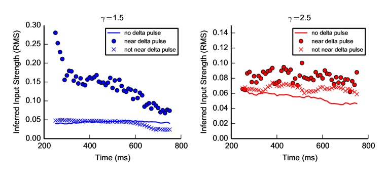
One possibility in using LFADS with inferred inputs (i.e. dimensionality of ) is that the data to be modeled is actually generated by an autonomous system, yet one, not knowing this fact, allows for an inferred input in LFADS. To study this case we utilized the four data RNNs described above, i.e. , and , with and without delta pulse inputs. We then trained an LFADS model for each of the four cases, with an inferred input of dimensionality 1, despite the fact that two of the four data RNNs generated their data autonomously. We trained all four models, and after training we examined the strength of the average inferred input, for each LFADS model ( as defined above). Our definition of strength is root-mean-square of the inferred input, averaged over an appropriate time window, . The results and details of this analysis are shown in Fig. 11. Importantly, the strength of the inferred input when pulses were not present in the data was similar to the magnitude of inferred input when pulses were present in the data but not in the specific window. Further, when inputs were present in the data and within the specific window, the magnitude of the inferred input was higher on average than cases without inputs.
5 Discussion
We have developed the LFADS algorithm for inferring latent dynamics from single-trial, high-dimensional neural spike trains. We tested the algorithm on synthetic datasets based on the nonlinear Lorenz attractor and a chaotic nonlinear RNN and showed that LFADS significantly outperforms other state-of-the-art algorithms in these examples. We note that if one wishes to study linear systems, a variety of optimal methods exist in the literature (e.g. Kalman filter).
The only explicit aspect of LFADS that ties it to neuroscience is the Poisson spiking process. By exchanging the Poisson distribution for a Gaussian emission distribution, for example, LFADS could be applied to all manner of time series data. However, there are further assumptions that implicitly tailor LFADS to neural data, which we outline in the next few paragraphs. For example, we use the temporal factors to implement a dimensionality bottleneck between the generator and the rates. This is based on the commonly observed phenomenon in neuroscience that the number of recorded units typically far exceeds the dimensionality of the data [6].
In many machine learning applications, all the inputs to the system are known. A particular aspect of neuroscience data is that the inputs typically are not known, so they must be inferred. (For example, even in primary visual cortex, the visual input from the world has already been transformed a number of times.) From a theoretical perspective, it may be extremely difficult to correctly factor observed data into features generated by a dynamical system and features generated by an feed-forward time-varying input, because the initial conditons or the feed-forward input are incompletely known. In applying LFADS to neuroscience data, regularizers on the complexity of either the dynamical system or the inferred inputs could be used to determine the relative weighting of these two factors. For example, in motor tasks network dynamics may be predominant, while inferred input may be more important in studies with extensive sensory input. In a neuroscience setting where input is so difficult to measure, it is not unreasonable to attempt to infer inputs, even if the results are only qualitatively correct, but caution should be exercised.
Often in deep sequence models, such as language models, the emission distribution (typically a softmax over discrete symbols) is viewed as a fundamental source of structural variability in the sequence. As a result, when these models are used for inference, a sample of the emission process is fed back to the network. In the case of LFADS applied to spiking neural data, we view the spikes as noisy observations of an underlying smooth process, so instantiating spikes and feeding them back into the generator would only serve to inject noise into the system (by assumption), not enhance structural variability. Thus, we do not do it. If one wanted to adapt LFADS to an application where the emission was not viewed as noise, then one would sample and feed that to the generator and controller at the next time step, instead of injected only to the controller.
While the primary motivation for the LFADS algorithm was inferring smooth latent variables, there is no reason why LFADS should be restricted to slow dynamics. The discrete-time RNN used in the algorithm can generate fast dynamics, so the fastest timescale that LFADS can produce is only limited by the binning or temporal resolution of the experimental spike counts. Relevant to this point, a clear sign that LFADS is beginning to overfit the data is the production of “spiky” rates with high-frequency changes that do not generalize to the held-out data, especially near the beginning of a trial or immediately after a strong input.
There are some obvious extensions and future directions to explore. First, an emissions model relevant to calcium imaging would be extremely useful for inferring neural firing rate dynamics underlying calcium signals. Second, in this contribution we implemented LFADS as a “smoother”, in Kalman filter language, that cannot run in real time. It would be interesting to adapt LFADS as a “filter” that could. Third, the LFADS generator could clearly be strengthed by stacking recurrent layers or adding a feed-forward deep net before the emissions distribution at each time step. Another extension would be to learn the dimensions of the inferred input and temporal factors automatically, instead of having them specified as predetermined hyper-parameters (e.g. nuclear norm minimization on the respective matrices). Finally, we can imagine an LFADS-type algorithm that leans more towards the feed-forward side of computation, but still has some recurrence. An application would be, for example, to explain short-term effects in visual processing. In this setting, the information transfer along the temporal dimension could be limited while expanding the information flow in the feed-forward direction.
6 Acknowledgments
We would like to thank John P. Cunningham, Laurent Dinh, and Jascha Sohl-Dickstein for extensive conversation. R.J. participated in this work while at Google, Inc. L.F.A.’s research was supported by US National Institutes of Health grant MH093338, the Gatsby Charitable Foundation through the Gatsby Initiative in Brain Circuitry at Columbia University, the Simons Foundation, the Swartz Foundation, the Harold and Leila Y. Mathers Foundation, and the Kavli Institute for Brain Science at Columbia University. C.P. was supported by a postdoctoral fellowship from the Craig H. Neilsen Foundation for spinal cord injury research.
7 Appendix
7.1 GRU equations
The GRU equations are as follows,
| (33) | ||||
| (34) | ||||
| (35) | ||||
| (36) |
with being the hidden state, denoting element-wise multiplication and denoting the logistic function. For clarity, we use the common variable symbols associated with the GRU, with the understanding that the variables represented here by these symbols are not the same variables as those in the general LFADS model description.
7.2 Further details of LFADS implementation.
While the general model is defined in the main manuscript, there were a number of details that aided in the optimization and generalization of the LFADS model applied to the datasets.
-
•
The matrix in the affine transformation is row-normalized to keep the factors relatively evenly scaled with respect to each other.
-
•
Following the authors in [1], we added a schedule on the KL divergence penalty so that the optimization does not quickly set the KL divergence to 0.
-
•
We experimented with the variance of the prior distribution for both the initial condition and inferred input distributions and settled on a value of 0.1, chosen to avoid saturating network nonlinearities.
- •
- •
-
•
As defined in eqn. 28, there is an information limiting regularizer placed on by virtue of minimizing the KL divergence between the approximate posterior over and the uninformative Gaussian prior.
-
•
We clipped our hidden state when any of its values went above a set threshold and used gradient clipping to avoid occasional pathological gradients.
References
- [1] Bowman, S. R., Vilnis, L., Vinyals, O., Dai, A. M., Jozefowicz, R., and Bengio, S. Generating sentences from a continuous space. Conference on Computational Natural Language Learning (CoNLL) (2016).
- [2] Carnevale, F., de Lafuente, V., Romo, R., Barak, O., and Parga, N. Dynamic control of response criterion in premotor cortex during perceptual detection under temporal uncertainty. Neuron 86, 4 (2015), 1067–1077.
- [3] Chung, J., Gulcehre, C., Cho, K., and Bengio, Y. Empirical evaluation of gated recurrent neural networks on sequence modeling. arXiv preprint arXiv:1412.3555 (2014).
- [4] Chung, J., Kastner, K., Dinh, L., Goel, K., Courville, A., and Bengio, Y. A recurrent latent variable model for sequential data. In Advances in Neural Information Processing Systems (NIPS) (2015).
- [5] Churchland, M. M., Cunningham, J. P., Kaufman, M. T., Foster, J. D., Nuyujukian, P., Ryu, S. I., and Shenoy, K. V. Neural population dynamics during reaching. Nature 487, 7405 (2012), 51–56.
- [6] Gao, P., and Ganguli, S. On simplicity and complexity in the brave new world of large-scale neuroscience. Current opinion in neurobiology 32 (2015), 148–155.
- [7] Gao, Y., Archer, E., Paninski, L., and Cunningham, J. P. Linear dynamical neural population models through nonlinear embeddings. arXiv preprint arXiv:1605.08454 (2016).
- [8] Gao, Y., Busing, L., Shenoy, K. V., and Cunningham, J. P. High-dimensional neural spike train analysis with generalized count linear dynamical systems. In Advances in Neural Information Processing Systems (2015), pp. 2044–2052.
- [9] Gregor, K., Danihelka, I., Graves, A., Rezende, D. J., and Wierstra, D. Draw: A recurrent neural network for image generation. arXiv preprint arXiv:1502.04623 (2015).
- [10] Hinton, G. E., Srivastava, N., Krizhevsky, A., Sutskever, I., and Salakhutdinov, R. R. Improving neural networks by preventing co-adaptation of feature detectors. arXiv preprint arXiv:1207.0580 (2012).
- [11] Kato, S., Kaplan, H. S., Schrödel, T., Skora, S., Lindsay, T. H., Yemini, E., Lockery, S., and Zimmer, M. Global brain dynamics embed the motor command sequence of caenorhabditis elegans. Cell 163, 3 (2015), 656–669.
- [12] Kingma, D. P., and Welling, M. Auto-encoding variational bayes. In Proceedings of the 2nd International Conference on Learning Representations (ICLR) (2013), no. 2014.
- [13] Kobak, D., Brendel, W., Constantinidis, C., Feierstein, C. E., Kepecs, A., Mainen, Z. F., Qi, X.-L., Romo, R., Uchida, N., and Machens, C. K. Demixed principal component analysis of neural population data. eLife 5 (2016), e10989.
- [14] Krishnan, R. G., Shalit, U., and Sontag, D. Deep kalman filters. arXiv preprint arXiv:1511.05121 (2015).
- [15] Macke, J. H., Buesing, L., Cunningham, J. P., Yu, B. M., Shenoy, K. V., and Sahani, M. Empirical models of spiking in neural populations. In Advances in neural information processing systems (2011), pp. 1350–1358.
- [16] Mante, V., Sussillo, D., Shenoy, K. V., and Newsome, W. T. Context-dependent computation by recurrent dynamics in prefrontal cortex. Nature 503, 7474 (2013), 78–84.
- [17] Petreska, B., Byron, M. Y., Cunningham, J. P., Santhanam, G., Ryu, S. I., Shenoy, K. V., and Sahani, M. Dynamical segmentation of single trials from population neural data. In Advances in neural information processing systems (2011), pp. 756–764.
- [18] Rajan, K., Harvey, C. D., and Tank, D. W. Recurrent network models of sequence generation and memory. Neuron 90 (2016), 1–15.
- [19] Rezende, D. J., Mohamed, S., and Wierstra, D. Stochastic backpropagation and approximate inference in deep generative models. In International Conference on Machine Learning, 2014 (2014).
- [20] Rigotti, M., Barak, O., Warden, M. R., Wang, X.-J., Daw, N. D., Miller, E. K., and Fusi, S. The importance of mixed selectivity in complex cognitive tasks. Nature 497, 7451 (2013), 585–590.
- [21] Sussillo, D., and Abbott, L. F. Generating coherent patterns of activity from chaotic neural networks. Neuron 63, 4 (2009), 544–557.
- [22] Sussillo, D., and Barak, O. Opening the black box: low-dimensional dynamics in high-dimensional recurrent neural networks. Neural computation 25, 3 (2013), 626–649.
- [23] Sussillo, D., Churchland, M. M., Kaufman, M. T., and Shenoy, K. V. A neural network that finds a naturalistic solution for the production of muscle activity. Nature neuroscience 18, 7 (2015), 1025–1033.
- [24] Yu, B. M., Cunningham, J. P., Santhanam, G., Ryu, S. I., Shenoy, K. V., and Sahani, M. Gaussian-process factor analysis for low-dimensional single-trial analysis of neural population activity. In Advances in neural information processing systems (2009), pp. 1881–1888.
- [25] Zaremba, W., Sutskever, I., and Vinyals, O. Recurrent neural network regularization. arXiv preprint arXiv:1409.2329 (2014).
- [26] Zhao, Y., and Park, I. M. Variational latent gaussian process for recovering single-trial dynamics from population spike trains. arXiv preprint arXiv:1604.03053 (2016).