Effective Distances for Epidemics Spreading on Complex Networks

Abstract

We show that the recently introduced logarithmic metrics used to predict disease arrival times on complex networks are approximations of more general network-based measures derived from random walks theory. Using the daily air-traffic transportation data we perform numerical experiments to compare the infection arrival time with this alternative metric that is obtained by accounting for multiple walks instead of only the most probable path. The comparison with direct simulations reveals a higher correlation compared to the shortest-path approach used previously. In addition our method allows to connect fundamental observables in epidemic spreading with the cumulant generating function of the hitting time for a Markov chain. Our results provide a general and computationally efficient approach using only algebraic methods.

I Introduction

Networks have received growing attention in the past decade particularly due to their applicability in describing a wide range of phenomena. Prominent examples are the mapping of the World Wide Web and structure of Internet, social and financial networks, epidemiology and language dynamics Barrat et al. (2008); Pastor-Satorras and Vespignani (2004); Pastor-Satorras et al. (2015); Castellano et al. (2009). In the context of epidemic spreading the prediction of outbreaks has become particularly important for public health issues. The rapid growth in the velocity of transportation means and frequency of movements has further increased the risk that global emergent diseases such as H1N1 Yang et al. (2009), SARS Colizza et al. (2007a) or EBOV Poletto et al. (2014), and more recently ZIKV Ioos et al. (2014), will spread worldwide. The underlying mobility networks are usually scale-free Barabási and Albert (1999). This implies the absence of an epidemic threshold Pastor-Satorras and Vespignani (2001) that allows any transmittable disease to spread through the global population.

The large amount of traffic data both at the local and global scale, which became available in recent years, provides a new opportunity to understand such processes. On the one hand numerical simulations of infection spreading offer a practical tool for estimating the infection arrival time Broeck et al. (2011). In this regard meta-population models Lentz et al. (2012); Colizza et al. (2007b); Colizza and Vespignani (2008) provide a reasonable tool for maintaining a high level of complexity in the simulation of pandemics Broeck et al. (2011). At the global scale the different subpopulations, defined by the nodes of the network, are cities that can be connected by directed or undirected fluxes of individuals, provided by the worldwide transportation network data. On the other hand algebraic methods give a solid foundation for drawing general conclusions and in many cases provide numerical instruments superior to direct simulations.

Figure 1: The global mobility network used in the simulations consisting of $V=3865$ airports and $E=51440$ flights dat .

In this work we introduce a network-based measure that generalizes the concept of distance and that provides fundamental insights into the dynamics of disease transmission as well as a efficent numerical estimation of the infection arrival time. We compare this effective distance bar with the numerical estimate of the transmission times using a meta-population model to validate the method. A series of papers have already been devoted to this problem Braunstein et al. (2003); Gautreau et al. (2007, 2008); Brockmann and Helbing (2013); Lawyer (2016). Most of them rely on the concept of most probable path, the shortest-path effective distance $D^{\text{SP}}_{ij}$ for each source $i$ and target $j$ in the network. The latter can be defined, for both directed and undirected networks, as the geodesic graph distance with edge weights given by the first moment of a Gumbel distributed variable which depends only on the network topology and the infection rate. This shortest-path approach however significantly overestimates the infection arrival times Gautreau et al. (2007); Crepey et al. (2006). A more realistic scenario takes into account all possible paths Gautreau et al. (2008) yielding the multiple-path distance $D^{\text{MP}}_{ij}$ which is better suited to estimate the arrival times of the infection. This method allows, at least in principle, to take into account all possible directed transmission paths although the computation becomes infeasible as their number grows exponentially with the the number of vertices in the network. The lack of a practical computational approach leads back to considering only the shortest path. A logarithmic ad-hoc edge weight transformation was introduced in Brockmann and Helbing (2013) by simply requiring that adding edges should translate to multiplying the associated probabilities. This follows the intuitive argument that a higher number of passengers reduces the separation distance between neighbouring nodes. This logarithmic transformation can be viewed as a log-space reduction Roosta (1982) and, how we will show later in the text, it can be derived as a special case of the shortest-path effective distance defined previously in Gautreau et al. (2007). The estimated arrival time $T^{\text{AR}}_{ij}$ from node $i$ to node $j$, obtained from numerical simulations, correlates highly with the shortest-path effective distance. Using this metrics the complexity of disease transmission can be understood in terms of circular waves propagating at constant velocity from the infected node at time zero to all other nodes in the network Brockmann and Helbing (2013). The measure we introduce here aims to generalize previous definitions by including all walks that connect source and target.

II Epidemiological model

Let us consider a meta-population susceptible-infected-removed dynamics $S\xrightarrow{\beta SI}I\xrightarrow{\mu I}R$, where $\beta$ and $\mu$ are the infection and recovery rate, respectively. The nodes of the meta-population network consists of subpopulations of constant size $N_{j}$, which divides into susceptible ($S_{j}$), infected ($I_{j}$) and removed ($R_{j}$) individuals

$$N_{j}=S^{(t)}_{j}+I^{(t)}_{j}+R^{(t)}_{j}.$$ (1)

In the meta-population in addition to the local SIR reaction dynamics, the movement of a host between populations $i$ and $j$ is governed by the master equation

$$\partial_{t}X_{j}^{(t)}=\sum_{i\neq j}\left(X^{(t)}_{i}Q_{ij}-X^{(t)}_{j}Q_{ji}\right).$$ (2)

Here, we introduced $X^{(t)}_{j}=\{S^{(t)}_{j},I^{(t)}_{j},R^{(t)}_{j}\}$ as a placeholder variable and the transition rates $Q_{ij}$ are defined as the conditional probability of a randomly chosen individual to jump from location $i$ to location $j$ within one time step

$$\mathbb{P}\left(X^{(t+\Delta t)}_{j}\middle|X^{(t)}_{i}\right)\approx Q_{ij}\Delta t,\qquad i\neq j.$$ (3)

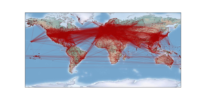
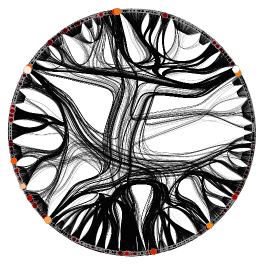
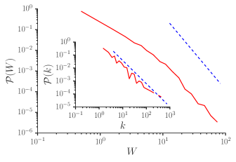
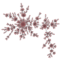
The transition rates $Q_{ij}$ can equivalently be defined in terms of the weighted adjacency matrix $A^{W}_{ij}$ as $Q_{ij}={A^{W}_{ij}}/{N_{i}}\in[0,1]$. The latter is obtained from the actual passenger fluxes between any two airports in the global mobility network used in the simulations dat . This network consists of $V=3865$ vertices (airports) and $E=51440$ directed edges (fluxes), with very broad degree and weight distributions, see Fig. 1 and  2, where the high heterogeneity in the network connectivity is graphically reproduced. For the network diameter we found $D=16$ (connecting Stuart Island to Narsaq Kujalleq Heliport) and the global clustering coefficient is $c=0.26\pm 0.01$. A peculiar feature of this network is that the antisymmetric part of the fluxes $\chi=A^{W}_{ij}-A^{W}_{ji}$ is vanishing to a high degree of accuracy so that it can be considered as undirected Barrat et al. (2004). The weighted adjacency matrix of the undirected air traffic network is then defined by $A^{W}_{ij}=A_{ij}W_{ij}$, where $A_{ij}$ is the adjacency matrix element and $W_{ij}\geq 0$ the corresponding weight. The symmetry in the adjacency matrix implies that for adjacent populations

$$A^{W}_{ij}=Q_{ij}N_{i}=Q_{ji}N_{j}=A^{W}_{ji}.$$ (4)

The Markov transition matrix associated to the network can be written in terms of both the fluxes $A^{W}_{ij}$ and the local transition rates $Q_{ij}$

$$P_{ij}=\frac{A^{W}_{ij}}{\sum_{j}A^{W}_{ij}}=\frac{Q_{ij}}{\sum_{j}Q_{ij}}.$$ (5)

and it is row stochastic by construction. From (4) we also have detailed balance

$$P_{ij}k^{W}_{i}=P_{ji}k^{W}_{j},$$ (6)

where we have introduced the weighted degree $k^{W}_{i}=\sum_{j}A^{W}_{ij}$, sometimes denoted as strength Caldarelli (2007), as the asymptotic probability distribution for the corresponding Markov chain. Thus using (6) we can rewrite (2), in terms of the compartment densities $x_{j}^{(t)}=X_{j}^{(t)}/N_{j}$ to obtain

$$\partial_{t}x_{j}^{(t)} =\frac{1}{N_{j}}\sum_{i\neq j}\left(x^{(t)}_{i}A^{W}_{ij}-x^{(t)}_{j}A^{W}_{ji}\right)$$ (7)

$$=\frac{k^{W}_{j}}{N_{j}}\sum_{i\neq j}P_{ji}\left(x^{(t)}_{i}-x^{(t)}_{j}\right).$$

Furthermore, we can remove the dependence on the population size $N_{j}$ by introducing a constant global mobility rate $\alpha$. This parameter is defined as the ratio $\alpha={\Phi}/{N}$, between the total daily passenger flux $\Phi=\sum_{ij}A_{ij}^{W}$ and the total population $N=\sum_{i}N_{i}$, i.e. the rate to leave a node for a randomly chosen individual. A local node dependent mobility rate can also be defined as

$$\alpha_{i}=\frac{\sum_{j}A^{W}_{ij}}{N_{i}}=\sum_{j}Q_{ij}.$$ (8)

In the global mobility network data the total traffic of each node, i.e. its weighted degree $k^{W}_{j}$, is with a good accuracy proportional to its population $N_{i}$ via the global mobility rate $\alpha$, thus in our case $\alpha_{i}=\alpha$ $\forall i$. The complete SIR dynamics of the Rvachev-Longini model Rvachev and Longini (1985); Brockmann and Helbing (2013) becomes

$$\begin{cases}\partial_{t}s_{j}^{(t)}=\Omega(\{s_{j}^{(t)}\})-\beta s_{j}^{(t)}i_{j}^{(t)}\\ \\ \partial_{t}i_{j}^{(t)}=\Omega(\{i_{j}^{(t)}\})+\beta s_{j}^{(t)}i_{j}^{(t)}-\mu i_{j}^{(t)}\\ \\ \partial_{t}r_{j}^{(t)}=\Omega(\{r_{j}^{(t)}\})+\mu i_{j}^{(t)}\end{cases}$$ (9)

where the mobility function for each compartment density $x_{j}=X_{j}/N_{j}$

$$\Omega(\{x_{j}\})=\alpha\sum_{i\neq j}P_{ji}\left(x_{i}^{(t)}-x_{j}^{(t)}\right),$$ (10)

accounts for diffusion along the nodes.

Integrating system (9) we obtain the contagion dynamics on the transportation network $A^{W}_{ij}$ with the global mobility rate $\alpha$ and the infection parameters $\beta$ and $\mu$. Finally, the arrival time ${T}^{\text{AR}}_{ij}$ for each source-target pair in the global mobility network is computed by considering a node $j$ infected as soon as one infected individual is present. After introducing the effective distance we use ${T}^{\text{AR}}_{ij}$ to compare the goodness of the different measures.

Figure 2: (Color online) (a) Circular representation of the global mobility network with vertex colors and size corresponding to its strenght $k_{i}^{W}$. (b) Normalized weight distribution $\mathcal{P}(W)\sim W^{-\gamma_{w}}$ with scaling exponent $\gamma_{w}=3.60\pm 0.14$. Inset: unweighted degree distribution $\mathcal{P}(k)\sim k^{-\gamma_{k}}$ with scaling exponent $\gamma_{k}=1.79\pm 0.10$. Scaling exponents are obtained using the method presented in Clauset et al. (2009).

III Effective network-based measures

The fundamental metric on a network is given by the (geodesic) shortest-path length over all paths $\Gamma_{ij}$ connecting node $i$ to node $j$. In a weighted network for each edge $(k,l)\in\Gamma_{ij}$ no node is visited more than once and contributes to the total length with its corresponding weight Barrat et al. (2008)

$$D_{ij}=\min_{\{\Gamma_{ij}\}}\sum_{\begin{subarray}{c}(k,l)\in\Gamma_{ij}\end{subarray}}\frac{1}{A^{W}_{kl}},$$ (11)

where the inverse is used because in our case a higher flux of passengers reduces the distance between two nodes. Starting from this definition it is possible to extend the notion of distance by replacing the adjacency matrix weight with an effective quantity that captures the essence of the problem of predicting when the disease will arrive at a certain place. In Gautreau et al. (2007) the authors defined the shortest-path distance $D^{\text{SP}}_{ij}$ by first considering the susceptible-infected model with only two cities, by then generalizing to arbitrary topologies. We first show how their analytical approach leads to an equivalent definition of effective distance used in Brockmann and Helbing (2013) and then we generalize it to more realistic propagation scenarios where all paths are taken into account.

Let us consider two susceptible populations $i$ and $j$ and place an infected individual in $i$ at time $t_{i}=0$. Assuming $Q_{ij}\Delta t\ll 1$ we can derive a probability density function for the infection hitting time $h_{j}$ to city $j$ of the Gumbel type Gautreau et al. (2007). The first moment of this distribution is given by

$$\mathinner{\langle{h_{j}}\rangle}_{i}=\frac{1}{\beta}\left(\ln\frac{\beta}{Q_{ij}}-\gamma_{e}\right),$$ (12)

where $\gamma_{e}\approx 0.5772$ is the Euler-Mascheroni constant and the average $\mathinner{\langle{\dots}\rangle}_{i}$ is taken over times starting at $t_{i}=0$. Using (5) we find

$$\beta\mathinner{\langle{h_{j}}\rangle}_{i} =\ln\frac{\beta}{\sum_{j}Q_{ij}}-\gamma_{e}-\ln\frac{Q_{ij}}{\sum_{j}Q_{ij}}$$ (13)

$$=\delta-\ln P_{ij},$$

where we assume the mobility rate (8) to be node independent, i.e. $\alpha_{i}=\alpha$ $\forall i$ and $\delta=\ln(\beta/\alpha)-\gamma_{e}$ is a dimensionless parameter. This result can easily be generalized to the SIR model and a network with an arbitrary number of nodes simply by minimizing the quantity $\mathinner{\langle{h_{l}}\rangle}_{k}$ for each consecutive link $(k,l)$ that belongs to the path $\Gamma_{ij}$ connecting source $i$ to target $j$. For the arbitrary heterogenous population and network topology with an arbitrary number of nodes by taking the minimum over all paths yields the shortest-path effective distance

$$D^{\text{SP}}_{ij}(\delta)\equiv\min_{\{\Gamma_{ij}\}}\sum_{\begin{subarray}{c}(k,l)\in\Gamma_{ij}\end{subarray}}\left(\delta-\ln P_{kl}\right)\approx(\beta-\mu)\mathinner{\langle{h_{j}}\rangle}_{i},$$ (14)

where for the SIR meta-population dynamics we have

$$\delta=\ln\left(\frac{\beta-\mu}{\alpha}\right)-\gamma_{e}.$$ (15)

Since each term in the sum is strictly positive, one can obtain the complete shortest-path distance matrix for each source and target pair using the Dijkstra algorithm Dijkstra (1959) in a time $\mathcal{O}(VE+V^{2}\log V)$, where $E$ and $V$ are the graph size and order, respectively. The effective distance defined in Brockmann and Helbing (2013) can then be recovered as a special case of (14) simply by setting the scale parameter $\delta$ to unity. This fact allows for a deeper and more complete understanding of this effective distance and offers a more solid explanation to the extremely high correlation with the infection arrival time found in Brockmann and Helbing (2013). The most important limitation of (14) is that only one path is considered, namely the path that in addition to minimizing the topological length also maximizes the probability associated to that. Thus in this scenario the contribution to the disease spread comes only from a single route. The effective infection arrival time $D^{\text{SP}}_{ij}(\delta)/\mathcal{V}^{\text{EF}}$, where $\mathcal{V}^{\text{EF}}\approx\beta-\mu$ is the linearized effective speed of the infection Gautreau et al. (2007); Brockmann and Helbing (2013), is in fact overestimated with respect to the simulations result $T^{\text{AR}}_{ij}$ Crepey et al. (2006).

Figure 3: (Color online) Correlation of the infection arrival times in days obtained from simulation of (9) with the shortest-path (light-blue circles) and the random-walk effective distance (violet squares). The source infected node $i$ is São Paulo Guarulhos International Airport and each point in the scatter plot corresponds to an airport $j$ in the global mobility network, with size proportional to its strength $k^{W}_{j}$. The mobility and epidemiological parameters are respectively $\alpha=0.028$ d^-1, $\beta=0.407$ d^-1 and $\mu=0.271$ d^-1 resulting in $\delta=1$. The Pearson correlation coefficients are $R^{2}_{\text{SP}}=0.96$ and $R^{2}_{\text{RW}}=0.99$.

To take into account the most realistic disease spread scenario one has to consider instead the multiplicity of transmission routes. For two distinct paths $\Gamma_{ij}$ and $\Gamma_{ij}^{\prime}$ connecting $i$ with $j$, the authors in Gautreau et al. (2008) found that a two path distance $D^{\text{2P}}_{ij}$ satisfies the equation

$$e^{-D^{\text{2P}}_{ij}}=e^{-D^{\Gamma_{ij}}}+e^{-D^{\Gamma_{ij}^{\prime}}},$$ (16)

where

$$D^{\Gamma_{ij}}(\delta)=\ln\left(\prod_{(k,l)\in\Gamma_{ij}}\frac{e^{\delta}}{P_{kl}}\right)$$ (17)

is the effective distance associated to the path $\Gamma_{ij}$ of arbitrary length, which corresponds to a Gumbel distributed hitting time. Relation (16) can then be easily generalized to an arbitrary number of multiple paths as

$$\exp\left(-D^{\text{MP}}_{ij}(\delta)\right)=\sum_{\{\Gamma_{ij}\}}\exp\left(-D^{\Gamma_{ij}}(\delta)\right),$$ (18)

so that we obtain

$$D^{\text{MP}}_{ij}(\delta) =-\ln\left(\sum_{\{\Gamma_{ij}\}}e^{-n_{ij}\delta}F_{ij}(\Gamma_{ij})\right).$$ (19)

Here we have defined the total probability associated to the path $\Gamma_{ij}$ as

$$F_{ij}(\Gamma_{ij})=\prod_{(k,l)\in\Gamma_{ij}}P_{kl}.$$ (20)

By grouping all probabilities associated to paths of the same length in the quantity $F_{ij}(n)=\sum_{|\Gamma_{ij}|=n}F_{ij}(\Gamma_{ij})$, we can replace in (19) the sum over all paths connecting $i$ to $j$ with a sum over integer path lengths to get

$$D^{\text{MP}}_{ij}(\delta)=-\ln\left(\sum_{n=1}^{n_{max}}e^{-n\delta}F_{ij}(n)\right),$$ (21)

where $n_{max}$ is the maximum path length in the network. If we select the path $\widetilde{\Gamma_{ij}}$ of length $\widetilde{n}$ that is associated to the dominant contribution, i.e. the path that maximize its associated probability and minimizes the topological path length, one recovers the shortest-path effective distance of (14)

$$\widetilde{D^{\text{MP}}_{ij}}(\delta)=\widetilde{n}\delta-\ln F_{ij}(\widetilde{n})=D^{SP}_{ij}(\delta).$$ (22)

Therefore the multiple-path distance gives a more accurate estimate of the infection arrival time, as it allows to take into account the most probable route as well as all possible alternative transmission routes. However since the total number of paths between $i$ and $j$ can scale as $\mathcal{O}(V!)$, the measure $D^{\text{MP}}_{ij}$ becomes computationally infeasible for large graphs.

Both measures ${D}^{\text{SP}}_{ij}$ and $D^{\text{MP}}_{ij}$ rely on the fact that the epidemic will spread along simple paths, i.e. routes that do not cross themselves. Here we follow instead a different approach and introduce a distance that includes all possible random walks from source to target. Relaxing the assumption of directed spread is equivalent to effectively erasing the memory from the system at each time step. This is achieved by including in (19) all walks $\Xi_{ij}$, which contrary to the paths $\Gamma_{ij}$, allow also already visited nodes. We define the random-walk effective distance by generalizing (19) as

$$D^{\text{RW}}_{ij}(\delta)=-\ln\left(\sum_{\{\Xi_{ij}\}}e^{-n_{ij}\delta}H_{ij}(\Xi_{ij})\right).$$ (23)

where $H_{ij}(\Xi_{ij})$ is the probability associated to a walk that starts in $i$ and arrives to $j$. As for the probabilities $F_{ij}$ we can group the probabilities associated to walks of the same length into $H_{ij}(n)=\sum_{|\Xi_{ij}|=n}H_{ij}(\Xi_{ij})$. The latter is precisely the hitting time probability for a Markov chain defined recursively as Norris (1998)

$$H_{ij}(n)=\sum_{k\neq j}P_{ik}H_{kj}(n).$$ (24)

Thus $H_{ij}(n)$ is simply the $n$-th power of the sub-transition probability matrix obtained by removing the $j$th row and column. Contrary to the multiple-path scenario now the walks are unbounded and so becomes $n_{max}$. Furthermore since each term in the sum (23) is positive, assuming the convergence of the sum, we can rearrange it as

$$D^{\text{RW}}_{ij}(\delta)=-\ln\left(\sum_{n=1}^{\infty}e^{-n\delta}H_{ij}(n)\right).$$ (25)

Figure 4: (Color online) Distribution of the Pearson coefficient $R^{2}$ considering all possible infection sources in the global mobility network for same parameters as in Fig. 3.

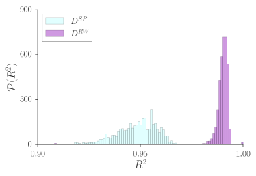
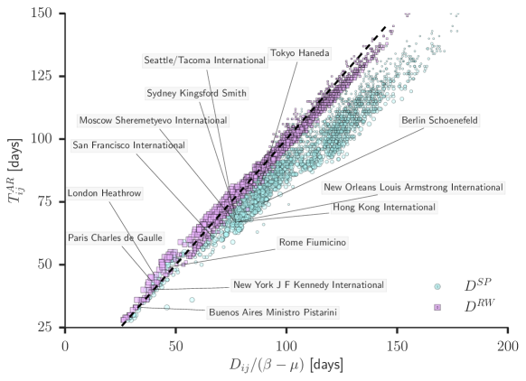
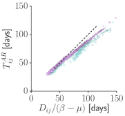
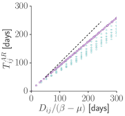
In Fig. 3 we use the Pearson correlation coefficient $R^{2}$ for quantifying the accuracy of the different measures using São Paulo airport as the source of the infection. Each dot in the scatter plot corresponds to an airport, which is labelled infected in the simulations when the the infection density is greater than zero. The high correlation with the infection arrival time found in Brockmann and Helbing (2013) using a shortest-path approach (light-blue) is improved when considering the random-walk effective distance (violet). The points on the dashed diagonal indicate a perfect agreement between the simulation and the effective distance. The correlation distribution considering all nodes in the network as initial infected seed shows that not only the measure proposed here possesses a higher averaged correlation but it is also more peaked around it, see Fig. 4.

Figure 5: (Color online) Correlation of the shortest-path (light-blue) and random-walk (violet) approach with the simulations arrival time for the the USA airport network used in Colizza et al. (2007b) (a) and its randomized (Erdős-Rényi) version (c). In (b) and (d) the corresponding networks visualisation consisting of $V=500$ nodes and $E=5960$ edges. Parameters as in Fig 3.

A remarkable interpretation of the random-walk effective distance can be found by noticing that by definition $D^{\text{RW}}_{ij}(\delta)=-\ln\mathinner{\langle{e^{-{\delta h_{j}}}}\rangle}_{i}$, where $h_{j}$ is the hitting time to node $j$ Kemeny et al. (1960). Thus, since $H_{ij}(0)=0$ for $i\neq j$, we have the correspondence

$$D^{\text{RW}}_{ij}(\delta)=-C_{ij}(-\delta),$$ (26)

with the logarithm of the moment generating function, i.e. the cumulant generating function of the hitting time in a Markov chain

$$C_{ij}(s)=\ln\left(\sum_{n=0}^{\infty}e^{ns}\ H_{ij}(n)\right)=\ln\mathinner{\langle{e^{sh_{j}}}\rangle}_{i}.$$ (27)

Hence one obtains the cumulants of the hitting time by differentiating the random-walk effective distance with respect to $\delta$ at $\delta=0$. This interesting correspondence allows one to rigorously relate epidemiological quantities such as the arrival time and the speed of infection in a reaction-diffusion model to the fluctuations of the hitting time. Then one can interpret $D^{\text{RW}}_{ij}(\delta)$ as a generalized free energy in a statistical physics perspective Kivimäki et al. (2014) and providing a more profound theoretical framework than the ad hoc measure proposed in Brockmann and Helbing (2013).

From the computational side, in order to evaluate the infinite sum in (25), we can restrict ourselves to the first non-vanishing contributions, which dominate due to the decreasing exponential in the walk length $n$. However, we can also solve the complete expression by rewriting (25) into a geometric series. This requires to vectorize $D^{\text{RW}}_{ij}$ with respect to the arrival node $j$ to obtain

$$d^{\text{RW}}_{i{(j)}}(\delta)=-\ln\left[\left(e^{\delta}\mathbf{I}(j|j)-\mathbf{P}(j|j)\right)^{-1}\mathbf{p}(j)\right]_{i},$$ (28)

where $\mathbf{P}(j|j)$ and $\mathbf{I}(j|j)$ are the transition and identity submatrices obtained by deleting row and column $j$ Zhang (2011), while $\mathbf{p}(j)$ is the $j$-th column of $\mathbf{P}$ with element $j$ removed. To obtain the previous expression we have used that for $\delta>0$, all eigenvalues of the matrix $e^{-\delta}\mathbf{P}(j|j)$ are strictly smaller than unity. For each arrival node the random-walk effective distance can then be obtained in polynomial time $\mathcal{O}(V^{3.4})$ using for instance the Coppersmith-Winograd algorithm for matrix inversion Coppersmith and Winograd (1987), making the problem of parallel transmission routes feasible even for large networks as the one used in our simulations.

Figure 6: (Color online) Correlation of the shortest-path (light-blue) and random-walk (violet) approach with the simulations arrival time for an unweighted Barabási-Albert network (a) and a two-dimensional lattice embedding (c) both consisting of $V=500$ nodes. In (b) and (d) the corresponding networks visualisation. The number of edges is respectively $E=998$ and $E=1000$. Parameters as in Fig 3.

For highly heterogeneous topologies, such as the air-traffic network Barrat et al. (2004), only a small number of paths contributes to ${D}^{\text{MP}}_{ij}$. Taking the limit of the dominant contribution in (23), which corresponds to selecting the dominant path in (19), allows one to neglect the sum over the walks (paths) and it yields as for (22)

$$\widetilde{D^{\text{RW}}_{ij}}(\delta)=-\ln\left(e^{-\widetilde{n}\delta}H_{ij}(\widetilde{n})\right)=D^{\text{SP}}_{ij}(\delta).$$ (29)

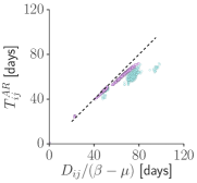
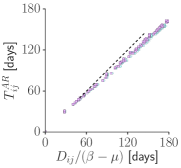
In Fig. 5 the comparison between the shortest-path and random-walk approach for the USA air-traffic network Colizza et al. (2007b) shows that the results presented here are robust also for Erdős-Rényi networks. The correlation coefficients are respectively $R^{2}_{\text{SP}}=0.99$ and $R^{2}_{\text{RW}}=1.00$ for the USA air-traffic network and $R^{2}_{\text{SP}}=0.94$ and $R^{2}_{\text{RW}}=1.00$ for the randomized Erdős-Rényi network. An higher correlation and stability of the random-walk approach is also observed in the case of artificial networks, as for unweighted Barabási-Albert Barabási and Albert (1999) and lattice models, see Fig. 6. The correlation coefficients for the latter are $R^{2}_{\text{SP}}=1.00$ and $R^{2}_{\text{RW}}=1.00$ for the Barabási-Albert network and $R^{2}_{\text{SP}}=0.99$ and $R^{2}_{\text{RW}}=1.00$ for the lattice.

IV Conclusions

In summary we have presented a generalization of the concept of effective distance by overcoming the restriction of simple path propagation of a disease. The proposed random-walk effective distance includes the previously defined shortest-path measure as a particular case. The remarkable correlation found with the infection arrival time can be explained as follows. The contribution of looped trajectories in the propagation of physical information is neglected thanks to the decreasing exponential in the walk length. The latter serves as damping such contributions for long walks, and in particular allows to neglect infinite loops contributions. In scenarios where multiple parallel paths are important, for instance in Erdős-Rényi graphs or regular lattices, the assumption of a single dominant path breaks down and the measure proposed here can be used as an efficient alternative. The predictive power of the random-walk effective distance can be used for containment strategies and estimation of arrival times for real global pandemics from the underlying networks topology. The random-walk metric can in fact be generally applied to any weighted and directed network besides the transportation ones, for instance in the context of social interactions and rumour spreading. For unweighted locally tree-like networks both the shortest-path and random-walk effective distances yield maximum correlation with the simulated arrival time, as the shortest path tends to dominate.

From a theoretical point of view our results show that the average infection arrival time in a meta-population model can be approximated by the cumulant generating function of the hitting time for a Markov chain. In fact, the generating function approach can also be used to formally derive the latter from the first moments of the Gumbel distribution Gautreau et al. (2007). The connection with the cumulant generating function allows for an interpretation within statistical physics. In particular this would explain how the different approaches are connected in terms of the entropy associated to paths of fixed length Kivimäki et al. (2014) Bavaud and Guex (2012). This observation links disease spreading on complex networks with a generic diffusion process. Further developments and extensions of our results include the generalization to temporal networks by considering a set of transition matrices, one for each time step Lentz et al. (2013); Koher et al. (2016).

References

- Barrat et al. (2008) A. Barrat, M. Barthélemy, and A. Vespignani, Dynamical Processes on Complex Networks (Cambridge University Press, 2008).
- Pastor-Satorras and Vespignani (2004) R. Pastor-Satorras and A. Vespignani, Evolution and Structure of the Internet: a Statistical Physics Approach (Cambridge University Press, 2004).
- Pastor-Satorras et al. (2015) R. Pastor-Satorras, C. Castellano, P. Van Mieghem, and A. Vespignani, Rev. Mod. Phys. 87, 925 (2015).
- Castellano et al. (2009) C. Castellano, S. Fortunato, and V. Loreto, Rev. Mod. Phys. 81, 591 (2009).
- Yang et al. (2009) Y. Yang, J. D. Sugimoto, M. E. Halloran, N. E. Basta, D. L. Chao, L. Matrajt, G. Potter, E. Kenah, and I. M. Longini, Science 326, 729 (2009).
- Colizza et al. (2007a) V. Colizza, A. Barrat, M. Barthélemy, and A. Vespignani, BMC Medicine 5, 1 (2007a).
- Poletto et al. (2014) C. Poletto, M. F. Gomes, A. P. y Piontti, L. Rossi, L. Bioglio, D. L. Chao, I. M. Longini, M. E. Halloran, V. Colizza, and A. Vespignani, Eurosurveillance 19 (2014).
- Ioos et al. (2014) S. Ioos, H.-P. Mallet, I. L. Goffart, V. Gauthier, T. Cardoso, and M. Herida, Medecine et Maladies Infectieuses 44, 302 (2014).
- Barabási and Albert (1999) A.-L. Barabási and R. Albert, Science 286, 509 (1999).
- Pastor-Satorras and Vespignani (2001) R. Pastor-Satorras and A. Vespignani, Phys. Rev. Lett. 86, 3200 (2001).
- Broeck et al. (2011) W. V. d. Broeck, C. Gioannini, B. Gonçalves, M. Quaggiotto, V. Colizza, and A. Vespignani, BMC Infectious Diseases 11, 1 (2011).
- Lentz et al. (2012) H. H. K. Lentz, T. Selhorst, and I. M. Sokolov, Phys. Rev. E 85, 066111 (2012).
- Colizza et al. (2007b) V. Colizza, R. Pastor-Satorras, and A. Vespignani, Nature Physics 3, 276 (2007b).
- Colizza and Vespignani (2008) V. Colizza and A. Vespignani, Journal of Theoretical Biology 251, 450 (2008).
- (15) Global mobility data of air traffic was provided by OAG (www.oag.com).
- (16) See http://barabasi.com/networksciencebook/.
- Braunstein et al. (2003) L. A. Braunstein, S. V. Buldyrev, R. Cohen, S. Havlin, and H. E. Stanley, Phys. Rev. Lett. 91, 168701 (2003).
- Gautreau et al. (2007) A. Gautreau, A. Barrat, and M. Barthélemy, Journal of Statistical Mechanics: Theory and Experiment 2007, L09001 (2007).
- Gautreau et al. (2008) A. Gautreau, A. Barrat, and M. Barthelemy, Journal of Theoretical Biology 251, 509 (2008).
- Brockmann and Helbing (2013) D. Brockmann and D. Helbing, Science 342, 1337 (2013).
- Lawyer (2016) G. Lawyer, BMC Infectious Diseases 16, 1 (2016).
- Crepey et al. (2006) P. Crepey, F. P. Alvarez, and M. Barthélemy, Phys. Rev. E 73, 046131 (2006).
- Roosta (1982) M. Roosta, Journal of Mathematical Analysis and Applications 88, 341 (1982).
- Barrat et al. (2004) A. Barrat, M. Barthelemy, R. Pastor-Satorras, and A. Vespignani, Proc. Nat. Acad. Sci. U.S.A. 101, 3747 (2004).
- Caldarelli (2007) G. Caldarelli, Scale-Free Neworks (Oxford University Press, 2007).
- Rvachev and Longini (1985) L. A. Rvachev and I. M. Longini, Mathematical Biosciences 75, 3 (1985).
- Clauset et al. (2009) A. Clauset, C. R. Shalizi, and M. E. J. Newman, SIAM Review 51, 661 (2009).
- Dijkstra (1959) E. W. Dijkstra, Numerische Mathematik 1, 269 (1959).
- Norris (1998) J. R. Norris, Markov Chains (Cambridge University Press, 1998).
- Kemeny et al. (1960) J. G. Kemeny, J. L. Snell, et al., Finite Markov Chains, Vol. 356 (van Nostrand Princeton, NJ, 1960).
- Kivimäki et al. (2014) I. Kivimäki, M. Shimbo, and M. Saerens, Physica A 393, 600 (2014).
- Zhang (2011) F. Zhang, Matrix theory: basic results and techniques (Springer Science & Business Media, 2011).
- Coppersmith and Winograd (1987) D. Coppersmith and S. Winograd, in Proceedings of the nineteenth annual ACM symposium on Theory of computing (ACM, 1987) pp. 1–6.
- Bavaud and Guex (2012) F. Bavaud and G. Guex, “Interpolating between random walks and shortest paths: A path functional approach,” in Social Informatics: 4th International Conference, SocInfo 2012, Lausanne, Switzerland, December 5-7, 2012. Proceedings, edited by K. Aberer, A. Flache, W. Jager, L. Liu, J. Tang, and C. Guéret (Springer Berlin Heidelberg, Berlin, Heidelberg, 2012) pp. 68–81.
- Lentz et al. (2013) H. H. Lentz, T. Selhorst, and I. M. Sokolov, Phys. Rev. Lett. 110, 118701 (2013).
- Koher et al. (2016) A. Koher, H. H. K. Lentz, P. Hövel, and I. M. Sokolov, PLoS ONE 11, 1 (2016).