A framework for the construction of generative models
for mesoscale structure in multilayer networks
Abstract
Multilayer networks allow one to represent diverse and coupled connectivity patterns — e.g., time-dependence, multiple subsystems, or both — that arise in many applications and which are difficult or awkward to incorporate into standard network representations. In the study of multilayer networks, it is important to investigate mesoscale (i.e., intermediate-scale) structures, such as dense sets of nodes known as communities, to discover network features that are not apparent at the microscale or the macroscale. The ill-defined nature of mesoscale structure and its ubiquity in empirical networks make it crucial to develop generative models that can produce the features that one encounters in empirical networks. Key purposes of such generative models include generating synthetic networks with empirical properties of interest, benchmarking mesoscale-detection methods and algorithms, and inferring structure in empirical multilayer networks. In this paper, we introduce a framework for the construction of generative models for mesoscale structures in multilayer networks. Our framework provides a standardized set of generative models, together with an associated set of principles from which they are derived, for studies of mesoscale structures in multilayer networks. It unifies and generalizes many existing models for mesoscale structures in fully-ordered (e.g., temporal) and unordered (e.g., multiplex) multilayer networks. One can also use it to construct generative models for mesoscale structures in partially-ordered multilayer networks (e.g., networks that are both temporal and multiplex). Our framework has the ability to produce many features of empirical multilayer networks, and it explicitly incorporates a user-specified dependency structure between layers. We discuss the parameters and properties of our framework, and we illustrate examples of its use with benchmark models for community-detection methods and algorithms in multilayer networks.
I Introduction
One can model many physical, technological, biological, financial, and social systems as networks. The simplest type of network is a graph Newman (2018), which consists of a set of nodes (which represent entities) and a set of edges between pairs of nodes that encode interactions between those entities. One can consider either unweighted graphs or weighted graphs, in which each edge has a weight that quantifies the strength of the associated interaction. Edges can also incorporate directions to represent asymmetric interactions or signs to differentiate between positive and negative interactions.
However, this relatively simple structure cannot capture many of the possible intricacies of connectivity patterns between entities. For example, in temporal networks Holme and Saramäki (2012); Holme (2015), nodes and/or edges change in time; and in multiplex networks Kivelä et al. (2014), multiple types of interactions can occur between the same pairs of nodes. To better account for the complexity, diversity, and dependencies in real-world interactions, one can represent such connectivity patterns using “multilayer networks” (see Section II.1) Kivelä et al. (2014); Boccaletti et al. (2014); Aleta and Moreno (2019); Bianconi (2018); Porter (2018). We use the term single-layer network (which is also called a “monolayer network” or a “graph”) for a multilayer network with a single layer (i.e., an ‘ordinary’ network), and we use the term “network” to refer to both single-layer and multilayer networks.
By using a single multilayer network instead of several independent single-layer networks, one can account for the fact that connectivity patterns in different layers often “depend” on each other. (We use the term dependent in a probabilistic sense throughout the paper: an object depends on if and only if .) For example, the connectivity patterns in somebody’s Facebook friendship network today may depend both on the connectivity patterns in that person’s Facebook friendship network last year (temporal) and on the connectivity patterns in that person’s Twitter followership network today (multiplex). Data sets that have multilayer structures are increasingly available (e.g., see Table 2 of Kivelä et al. (2014)). A natural type of multilayer network consists of a sequence of dependent single-layer networks, where layers may correspond to different temporal snapshots, different types of related interactions that occur during a given time interval, and so on. Following existing terminology Domenico et al. (2015); Porter (2018), we refer to an instance of a node in one “layer” as a “state node” (see Section II.1).
There is a diverse set of models for multilayer networks. (We overview them in Section II.3.) Many of these models take a specific type of dependency (e.g., temporal) as their starting point. In the present paper, we introduce a framework for the construction of generative models for multilayer networks that incorporate a wide variety of structures and dependencies. It is broad enough to unify many existing, more restrictive interlayer specifications, but it is also easy to customize to yield multilayer network models for many specific cases of interest. Key purposes of such generative models include (1) generating synthetic networks with empirical features of interest, (2) benchmarking methods and algorithms for detecting mesoscale structures, and (3) inferring structure in empirical multilayer networks.
A unifying framework
A key feature of multilayer networks is their flexibility, which allows one to incorporate many different types of data as part of a single structure. In this spirit, our goal is to provide a general, unifying framework that enables users to construct generative models of multilayer networks with a large variety of features of interest in empirical multilayer networks by appropriately constraining the parameter space. We accomplish this in two consecutive steps. First, we partition the set of state nodes of a multilayer network. Second, we allocate edges, given a multilayer partition. We focus on modeling dependency at the level of partitions (as was done in Ghasemian et al. (2016)), rather than with respect to edges. Additionally, we treat the process of generating a multilayer partition separately from that of generating edges for a given multilayer partition. This modular approach yields random structures that can capture a wide variety of interlayer-dependency structures, including temporal and/or multiplex networks, appearance and/or disappearance of entities, uniform or nonuniform dependencies between state nodes from different layers, and others. For a specified interlayer-dependency structure, one can then use any (single-layer or multilayer) network model with a planted partition (i.e., a planted-partition network model) to generate a wide variety of network features, including weighted edges, directed edges, and spatially-embedded layers.
The flexibility of our framework to generate multilayer networks with a specified dependency structure between different layers makes it possible to (1) gain insight into whether, when, and how to build interlayer dependencies into methods for studying many different types of multilayer networks and (2) generate tunable “benchmark models” that allow a principled comparison for community-detection (and, more generally, “meso-set-detection”) tools for multilayer networks, including for complicated situations that arise in many applications (such as networks that are both temporal and multiplex) but thus far have seldom or never been studied. In many benchmark models, one plants a partition of a network into well-separated “meso-sets” (e.g., communities), and one thereby imposes a so-called “ground truth” (should one wish to use such a notion) Peel et al. (2017) that a properly deployed meso-set-detection method ought to be able to find. Benchmark networks with known structural properties can be important for (1) analyzing and comparing the performance of different meso-set-detection tools; (2) better understanding the inner workings of meso-set-detection tools; and (3) determining which tool(s) may be most appropriate in a given situation.
One can also use our framework to generate synthetic networks with desired empirical properties, to generate null networks, and to explore “detectability limits” of mesoscale structures. (See, for example, the study of detectability thresholds in Ghasemian et al. (2016) for a model that is a special case of our framework.) With some further work, it is also possible to use our framework to develop models for statistical inference. In our concluding discussion (see Section VII), we suggest directions for how to apply our framework to the task of statistical inference. Our intention in designing such a flexible framework is to ensure that the generative models that it provides remain useful as researchers consider progressively more general multilayer networks in the coming years.
Paper outline
Our paper proceeds as follows. In Section II, we give an introduction to multilayer networks, overview mesoscale structure in networks, and review related work on generative models for mesoscale structure. In Section III, we formally introduce the notation that we use throughout the paper. In Section IV, we explain how we generate a multilayer partition with a specified dependency structure between layers. We also give examples of how to constrain the parameter space of our framework to generate several different types of multilayer networks and discuss what we expect to be common use cases (including temporal structure Sarzynska et al. (2015); Ghasemian et al. (2016); Pamfil et al. (2019a) and multiplex structure Domenico et al. (2015); Pamfil et al. (2019a)) in detail. In Section V, we describe how we generate edges that are consistent with the planted partition. In Section VI, we illustrate the use of our framework as a way to construct benchmark models for multilayer community detection. In Section VII, we summarize our main results and briefly discuss possible extensions of our work to enable statistical inference on empirical multilayer networks with our framework.
Along with this paper, we include code Jeub and Bazzi (2016–2019) that users can modify to readily incorporate different types of “null distributions” (see Section IV.1), “interlayer-dependency structures” (see Section IV.2), and planted-partition network models (see Section V). The model instantiations that one needs for generating the figures in Section VI are available at https://dx.doi.org/10.5281/zenodo.3304059.
II Background and related work
II.1 Multilayer networks
The simplest type of network is a graph , where is a set of nodes (which correspond to entities) and is a set of edges. Using a graph, one can encode the presence or absence of connections (the edges) between entities (the nodes). However, in many situations, it is desirable to include more detailed information about connections between entities. A common extension is to allow each edge to have a weight, which one can use to represent the strength of a connection. We assign a weight to each edge using a weight function .
As we mentioned in Section I, one can also generalize the notion of a graph to encode different aspects of connections between entities, such as connections at different points in time or multiple types of relationships. We adopt the framework of multilayer networks Kivelä et al. (2014); Domenico et al. (2013); Bianconi (2018); Aleta and Moreno (2019); Porter (2018) to encode such connections in a network. In a multilayer network, a node can be present in a variety of different states, where each state is also characterized by a variety of different aspects. In this setting, edges connect state nodes, each of which is the instantiation of a given node in a particular state. The set of all state nodes of a given entity corresponds to a single physical node (which represents the entity), and the set of all state nodes in a given state is in one layer of a multilayer network. In the remainder of this paper, we use the terms “physical node” and “node” interchangeably and the terms “layer” and “state” interchangeably. One can think of the aspects as features that one needs to specify to identify the state of a node. In other words, a state is a collection of exactly one element from each aspect. For convenience, we introduce a mapping that assigns an integer label to each element of an aspect. That is, we map the elements of the aspect to the elements of a set of integers. Aspects can be unordered (e.g., social-media platform) or ordered (e.g., time). Most empirical investigations of multilayer networks focus on a single aspect (e.g., temporal Bazzi et al. (2016); Betzel and Bassett (2017); Hric et al. (2018) or multiplex Cantini et al. (2015); Bacco et al. (2017); Stanley et al. (2016)). However, many real-world situations include more than one aspect (e.g., a multiplex network that changes over time). For an ordered aspect, we require that the mapping respects the order of the aspect (e.g., for time, where is a set of discrete time points). A multilayer network can include an arbitrary number of ordered aspects and an arbitrary number of unordered aspects, and one can generalize these ideas further (e.g., by introducing a time horizon) Kivelä et al. (2014).
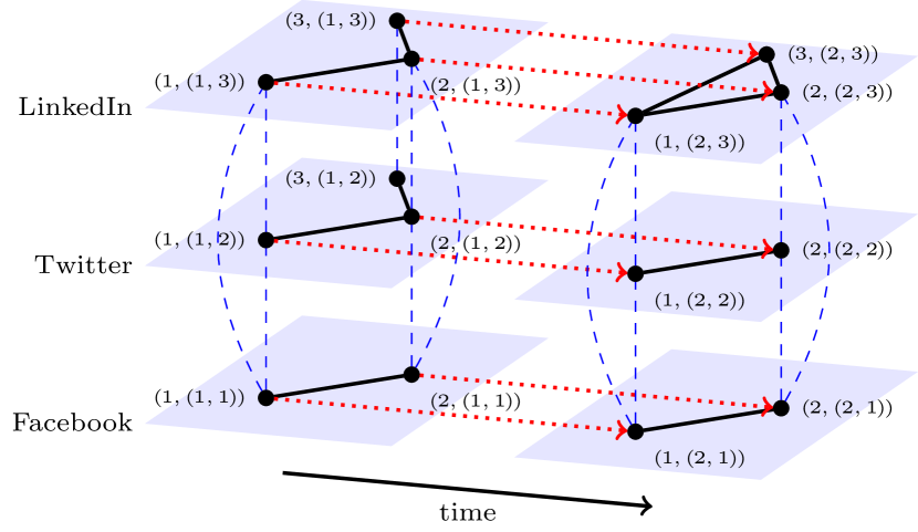
To illustrate the above ideas, consider a hypothetical social network with connections on multiple social-media platforms (‘Facebook’, ‘Twitter’, and ‘LinkedIn’) between the same set of people at different points in time. In this example network, there are two aspects: social-media platform and time. (One can consider ‘type of connection’ (e.g., ‘friendship’ and ‘following’) as a third aspect, but we restrict our example to two aspects for simplicity.) The first aspect is ordered, and the number of its elements is equal to the number of time points or time intervals. (For simplicity, we often refer simply to “time points” in our discussions.) The second aspect is unordered and consists of three elements: ‘Facebook’ (which we label with the integer “”), ‘Twitter’ (which we label with “”), and ‘LinkedIn’ (which we label with “”). If we assume that the time resolution is daily and spans the year , an example of a state is the tuple (‘01-Jan-2010’, ‘Twitter’), which is in our shorthand notation. We show a multilayer representation of this example social network in Fig. 1.
Edges in a multilayer network can occur either between nodes in the same state (i.e., intralayer edges) or between nodes in different states (i.e., interlayer edges). An example of an intralayer edge in Fig. 1 is (1, (1, 1)) (2, (1, 1)), indicating that entity is friends with entity on Facebook at time . All interlayer edges in Fig. 1 are diagonal (because they connect state nodes that correspond to the same physical node). Interlayer edges between layers at different times for a given social-media platform are ordinal (because they connect state nodes with successive time labels 111It is also possible to have ordinal layering in aspects other than time.) and directed. Interlayer edges between concurrent layers that correspond to different social-media platforms are categorical and undirected. (In this example, such edges occur between state nodes from all pairs of concurrent layers, although one can envision situations in which interlayer edges occur only between state nodes from a subset of such layers.) An example of an ordinal intralayer edge in Fig. 1 is (1, (1, 1)) (1, (2, 1)), indicating a connection from entity in Facebook at time to entity in Facebook at time . An example of a categorical intralayer edge in Fig. 1 is (1, (1, 1)) (1, (1, 2)), indicating a connection between node in Facebook at time and node in Twitter at time . One can also imagine other types of interlayer edges in an example like the one in Fig. 1, as there may be edges between state nodes at successive times and different social-media platforms (e.g., ).
II.2 Mesoscale structures in networks
Given a (single-layer or multilayer) network representation of a system, it is often useful to apply a coarse-graining technique to investigate features that lie between those at the microscale (e.g., nodes, pairwise interactions between nodes, or local properties of nodes) and those at the macroscale (e.g., total edge weight, degree distribution, or mean clustering coefficient) Newman (2018). One thereby studies mesoscale features such as community structure Porter et al. (2009); Fortunato and Hric (2016); Rossetti and Cazabet (2018); Cherifi et al. (2019), core–periphery structure Csermely et al. (2013); Rombach et al. (2017), role structure Rossi and Ahmed (2015), and others.
Our framework can produce multilayer networks with any of the above mesoscale structures. Notwithstanding this flexibility, an important situation is multilayer networks with “community structure”, which are the most commonly studied type of mesoscale structure Newman (2018). Community detection is part of the standard toolkit for studying single-layer networks Porter et al. (2009); Fortunato (2010); Fortunato and Hric (2016), and efforts at community detection in multilayer networks have led to insights in applications such as brain and behavioral networks in neuroscience Vaiana and Muldoon (2018), financial correlation networks Bazzi et al. (2016), committee and voting networks in political science Mucha and Porter (2010); Mucha et al. (2010), networks of interactions between bacterial species Stanley et al. (2016), disease-spreading networks Sarzynska et al. (2015), social networks in Indian villages Omodei and Arenas (2016), and much more.
Loosely speaking, a community in a network is a set of nodes that are “more densely” connected to each other than they are to nodes in the rest of the network Porter et al. (2009); Fortunato (2010); Fortunato and Hric (2016); Schaub et al. (2017); Jeub et al. (2015). Typically, a ‘good community’ should be a set of nodes that are ‘surprisingly well-connected’ in some sense, but what one means by ‘surprising’ and ‘well-connected’ is often application-dependent and subjective. In many cases, a precise definition of “community” depends on the method that one uses to detect communities. In particular, many popular community-detection approaches in single-layer and multilayer networks define communities as sets in a partition of a network that optimizes a quality function such as modularity Fortunato and Hric (2016); Newman (2018, 2006); stability Petri and Expert (2014); Lambiotte et al. (2015); Delvenne et al. (2010); Infomap and its variants Domenico et al. (2015); Rosvall and Bergstrom (2008); likelihood functions that are derived from stochastic block models (SBMs), which are models for partitioning a network into sets of nodes with statistically homogeneous connectivity patterns Holland et al. (1983); Karrer and Newman (2011); Stanley et al. (2016); Peixoto (2015); Kloumann et al. (2016); and others Kivelä et al. (2014); Jeub et al. (2017); Wilson et al. (2017). In this paper, we refer to a partition of the set of nodes of a single-layer network as a single-layer partition and to a partition of the set of state nodes of a multilayer network as a multilayer partition. The two primary differences between a community in a multilayer partition and a community in a single-layer partition are that (1) the former can include state nodes from different layers; and (2) “induced communities” (see Section III) in one layer of a multilayer network may depend on connectivity patterns in other layers. For many notions of (single-layer or multilayer) community structure — including the most prominent methods — one cannot exactly solve a community-assignment problem in polynomial time (unless P = NP) Fortunato (2010); Brandes et al. (2008); Jacobs and Clauset (2014); Ghasemian et al. (2019); and popular scalable heuristics currently have few or no theoretical guarantees on how closely an identified partition resembles an optimal partition. These issues apply more generally to the field of cluster analysis, such as in graph partitioning Schaeffer (2007), and many of the problems that plague community detection also apply to detecting other kinds of mesoscale structures.
Throughout our paper, to make it clear which results and observations apply to community structure in particular and which apply to mesoscale structure more generally, we use the term “community” when referring to a set in a partition of the set of nodes (or the set of state nodes) of a network that corresponds to community structure and the term “meso-set” (see Section III) when referring to a set in a partition that corresponds to any type of mesoscale structure. (In particular, a community is a type of meso-set.)
II.3 Generative models for mesoscale structure
The ubiquity and diversity of mesoscale structures in empirical networks make it crucial to develop generative models of mesoscale structure that can produce features that one encounters in empirical networks. Broadly speaking, the goal of such generative models is to construct synthetic networks that resemble real-world networks when one appropriately constrains and/or calibrates the parameters of a model using information about a scenario or application. Generative models of mesoscale structure can serve a variety of purposes, such as (1) generating benchmark network models for comparing meso-set-detection methods and algorithms Lancichinetti and Fortunato (2009); Lancichinetti et al. (2008); Granell et al. (2015); Ghasemian et al. (2016); Condon and Karp (2000); Girvan and Newman (2002); (2) undertaking statistical inference on empirical networks Ghasemian et al. (2016); Karrer and Newman (2011); Peixoto (2018); (3) generating synthetic networks with a desired set of properties Jeub et al. (2018); Bacco et al. (2017); (4) generating null models to take into account available information about an empirical network Paul and Chen (2016a); and (5) investigating “detectability limits” for mesoscale structure, as one can plant partitions that, under suitable conditions, cannot subsequently be detected algorithmically, despite the fact that they exist by construction Decelle et al. (2011); Ghasemian et al. (2016); Taylor et al. (2017).
One of the main challenges in constructing a realistic generative model (even for single-layer networks) is the breadth of possible empirical features in networks. The available generative models for mesoscale structure in single-layer networks usually focus on replicating a few empirical features at a time (rather than all of them at once): heterogeneous degree distributions and community-size distributions Lancichinetti et al. (2008); Karrer and Newman (2011); Orman et al. (2013), edge-weight distribution Lancichinetti and Fortunato (2009); Aicher et al. (2014); Peixoto (2018), spatial embeddedness Sarzynska et al. (2015); Newman and Peixoto (2015), and so on. Multilayer networks inherit all of the empirical features of single-layer networks, and they also have a key additional one: dependencies between layers. These interlayer dependencies can be ordered (as in most models of temporal networks), unordered (as in multiplex networks), combinations of these, or something more complicated. However, despite this variety, existing generative models for mesoscale structure in multilayer networks allow only a restrictive set of interlayer dependencies. They assume either a temporal structure Sarzynska et al. (2015); Granell et al. (2015); Ghasemian et al. (2016); Zhang et al. (2017); Hulovatyy and Milenković (2016); Pasta and Zaidi (2016), a simplified multiplex structure with the same planted partitions across all layers Peixoto (2015); Paul and Chen (2016b); Vallès-Català et al. (2016); Barbillon et al. (2016); Bacco et al. (2017), or independent groups of layers such that layers in the same group have identical planted partitions Domenico et al. (2015); Stanley et al. (2016). Using an alternative approach, a very recent model is able to generate multilayer partitions that satisfy the constraint that nonempty induced meso-sets in different layers that correspond to the same meso-set in the multilayer partition are identical Huang et al. (2019). Recent work Pamfil et al. (2019a) on the link between multilayer modularity maximization and maximum-likelihood estimation of multilayer SBMs allows either temporal or multiplex interlayer dependencies with induced partitions that can vary across layers, but it makes restrictive assumptions on interlayer dependencies (e.g., all layers have the same set of nodes, interdependencies are “diagonal” and “layer-coupled”, and so on). Importantly, in all aforementioned generative models of mesoscale structure in multilayer networks, interlayer dependencies are either (1) not explicitly specifiable or (2) special cases of the framework that we discuss in the present paper.
III Notation
We now present a comprehensive set of notation for multilayer networks. Different subsets of notation are useful for different situations.
We consider a multilayer network with nodes (i.e., physical nodes) and layers (i.e., states). We use to denote the number of aspects and to denote the labels of the aspect (where ). We use to denote the set of ordered aspects and to denote the set of unordered aspects. For each ordered aspect , we assume that the labels reflect the order of the aspect. That is, for all , we require that if and only if precedes . We say that a multilayer network is fully-ordered if , unordered if , and partially-ordered otherwise. The set of states is the Cartesian product of the aspects, where a state is an integer-valued vector of length and each entry specifies an element of the corresponding aspect. Note that .
We use to denote the state node (i.e., “node-layer tuple” Kivelä et al. (2014)) of physical node in state . We include a state node in if and only if the corresponding node exists in that state. The edges in a multilayer network connect state nodes to each other. We use to denote a directed edge from to . For two state nodes, and , that are connected to each other via a directed edge , we say that is an in-neighbor of and is an out-neighbor of . We categorize the edges into intralayer edges , which have the form and link entities and in the same state , and interlayer (i.e., coupling) edges , which have the form for . We thereby decompose the edge set as .
We define a weighted multilayer network by introducing a weight function (analogous to the weight function for weighted single-layer networks), which encodes the edge weights within and between layers. For an unweighted multilayer network, for all . We encode the connectivity pattern of a multilayer network using an adjacency tensor , which is analogous to the adjacency matrix for single-layer networks, with entries
| (1) |
Note that is a graph on the state nodes of the multilayer network . We refer to as the flattened network of . The adjacency matrix of the flattened network is the “supra-adjacency matrix” Kivelä et al. (2014); Domenico et al. (2014, 2013); Gómez et al. (2013) of the multilayer network. One obtains a supra-adjacency matrix by flattening 222 Flattening (i.e., ‘matricizing’) Kivelä et al. (2014) a tensor entails writing its entries in matrix form. Consequently, starting from a tensor with elements , one obtain a matrix with entries , where there are bijective mappings between the indices. an adjacency tensor (see Eq. 1) of a multilayer network. The multilayer network and the corresponding flattened network encode the same information Kolda and Bader (2009); Kivelä et al. (2014), provided one keeps track of the correspondence between the nodes in the flattened network and the physical nodes and layers of the multilayer network. In a similar vein, aspects provide a convenient way to keep track of the correspondence between state nodes and, for example, temporal and multiplex relationships.
We denote a multilayer partition with sets by , where and for . We represent a partition using a partition tensor with entries , where if and only if the state node is in the set . We refer to a partition of a temporal network (a common type of multilayer network) as a temporal partition and a partition of a multiplex network (another common type of multilayer network) as a multiplex partition. A multilayer partition induces a partition on each layer, where . We refer to a set of a partition as a meso-set, to as the induced partition of on layer , and to as the induced meso-set of on layer . A community is a set in a partition that corresponds to community structure. We call the label of meso-set . One way to examine overlapping meso-sets is by identifying multiple state nodes from a single layer with the same physical node.
IV Generating multilayer partitions
The systematic analysis of dependencies between layers is a key motivation for analyzing a single multilayer network, instead of examining several single-layer networks independently. The goal of our partition-generation process is to model interlayer dependency in a way that can incorporate diverse types of dependencies. We now motivate our partition-modeling approach, and we describe it in detail in Sections IV.1, IV.2, IV.3, and IV.4.
The complexity of dependencies between layers can make it difficult to explicitly specify a joint probability distribution for meso-set assignments, especially for unordered or partially-ordered multilayer networks. To address this issue, we require only the specification of conditional probabilities for a state node’s meso-set assignment, given the assignments of all other state nodes. The idea of conditional models is old and follows naturally from Markov-chain theory Bartlett (1978); van Buuren (2018). Specifying conditional models (which capture different dependency features separately) rather than joint models (which try to capture many dependency features at once) is convenient for numerous situations. For example, conditionally specified distributions have been applied to areas such as spatial data modeling Besag (1974), imputation of missing data van Buuren (2018), secure disclosure of information Fienberg and Slavkovic (2005), dependence networks for combining databases from different sources Heckerman et al. (2000), and Gibbs sampling Gelfand (2000); Hobert and Casella (1998).
A problem with conditional models is that the different conditional probability distributions are not necessarily compatible, in the sense that there may not exist a joint distribution that realizes all conditional distributions Hobert and Casella (1998); Arnold and Press (1989); Chen (2010); Chen and lp (2015); Heckerman et al. (2000). Although several methods have been developed in recent years for checking the compatibility of discrete conditional distributions, these either make restrictive assumptions on the conditional distributions or have scalability constraints that significantly limit practical use Kuo and Wang (2011); van Buuren (2018). Nevertheless, the employment of conditional models (even if potentially incompatible) is common Kuo and Wang (2017), and they have been useful in many applications, provided that one cautiously handles any potential incompatibility van Buuren (2018). For our use case, potential incompatibility arises for unordered or partially-ordered multilayer networks. An issue that can result from it is the non-uniqueness of a joint distribution. We carefully design our partition-generation process such that it is well-defined irrespective of whether conditional distributions are compatible. In particular, we show that convergence is guaranteed and we address non-uniqueness by appropriately sampling initial conditions (see Appendix B). We also suggest empirical checks to ensure that a generated partition reflects planted interlayer dependencies.
In our framework, we define conditional probabilities in two parts: we separately specify (1) independent layer-specific random components and (2) interlayer dependencies. For a choice of interlayer dependencies, there are several features that one may want to allow in a multilayer partition. These include variation in the numbers and sizes of meso-sets across layers (e.g., meso-sets can gain state nodes, lose state nodes, appear, and disappear) and the possibility for these meso-set variations to incorporate features of the application at hand. (For example, in a temporal network, one may not want a meso-set to reappear after it disappears.) We ensure that such features are possible for any choice of interlayer dependency via independent layer-specific null distributions that specify the set of possible meso-set assignments for each layer and determine the expected size and expected number of meso-sets in the absence of interlayer dependencies.
Interlayer dependencies should reflect the type of multilayer network that one is investigating. For example, in a temporal network, dependencies tend to be stronger between adjacent layers and weaker for pairs of layers that are farther apart. It is common to assume that interlayer dependencies are uniform across state nodes for a given pair of layers (i.e., interlayer dependencies are “layer-coupled” Kivelä et al. (2014)) and occur only between state nodes that correspond to the same physical node (i.e., interlayer dependencies are “diagonal” Kivelä et al. (2014)) Mucha et al. (2010); Stanley et al. (2016); Taylor et al. (2017); Bassett et al. (2011); Bazzi et al. (2016); Sarzynska et al. (2015); Gómez et al. (2013); Domenico et al. (2014). However, these assumptions are too restrictive in many cases (e.g., situations in which dependencies are state-node-dependent or in which dependencies exist between state nodes that do not correspond to the same physical node) Domenico et al. (2015); Jeub et al. (2017); Buldú and Porter (2017); Aslak et al. (2018); Valdano et al. (2015); Barbillon et al. (2016). To ensure that one can relax these assumptions, we allow dependencies to be specified at the level of state nodes (or at the level of layers, when a user assumes that dependencies are layer-coupled). We encode these interlayer dependencies in a user-specified interlayer-dependency tensor that determines the extent to which a state node’s meso-set assignment in one layer “depends directly” on the assignment of state nodes in other layers (see Sections IV.2 and IV.3). Our independence assumption on the null distributions allows us to encode all of the interlayer dependencies in a single object (an interlayer-dependency tensor). The entries of an interlayer-dependency tensor specify an “interlayer-dependency network” and correspond to the causal links for the flow of information (in the information-theoretic sense) between different layers of a multilayer network. Therefore, they should reflect any constraints that one wishes to impose on the direct flow of information between layers. Longer paths in an interlayer dependency network yield indirect dependencies between structures in different layers.
After specifying the interlayer-dependency structure, we define the conditional meso-set assignment probabilities such that we either sample a state node’s meso-set assignment from the corresponding null distribution or obtain it by copying the assignment of another state node (based on the interlayer-dependency tensor). Using these conditional probabilities, we define an iterative update process on the meso-set assignments of state nodes to generate multilayer partitions with dependencies between induced partitions in different layers. When updating the meso-set assignments of state nodes, we respect the order of an aspect (e.g., temporal ordering). For a fully-ordered multilayer network, our update process reduces to sequentially sampling an induced partition for each layer based on the induced partitions of previous layers. For an unordered multilayer network, our update process defines a Markov chain on the space of multilayer partitions. We sample partitions from a stationary distribution of this Markov chain. This sampling strategy is known as (pseudo-)Gibbs sampling Gelfand (2000); Hobert and Casella (1998); Kuo and Wang (2017); Heckerman et al. (2000). (We use the word “pseudo” because the conditional probabilities that we use to define the Markov chain are not necessarily compatible.) For a partially-ordered multilayer network, our update process combines these two sampling strategies.
In Section IV.1, we describe possible choices for the independent layer-specific null distributions. In Section IV.2, we explain our framework for generating a multilayer partition with general interlayer dependencies. In Section IV.3, we focus on the specific situation in which interlayer dependencies are layer-coupled and diagonal, and we also assume that a physical node is present in all layers (i.e., the network is “fully interconnected” Kivelä et al. (2014)). In Section IV.4, we illustrate the properties of example temporal and multiplex partitions that are generated by models that we construct from our framework. Additionally, we take advantage of the tractability of the special case of temporal networks to highlight some of its properties analytically.
IV.1 Null distribution
We denote the null distribution of layer by and the set of all null distributions by . A simple choice for the null distributions is a categorical distribution, where for each layer and each meso-set label , we fix the probability that an arbitrary state node in layer is assigned to a meso-set in the absence of interlayer dependencies. That is,
| (2) |
where is the total number of meso-sets in the multilayer partition and for all . The set is the set of meso-set labels, and the support of a null distribution is the set of labels that have nonzero probability. In the absence of interlayer dependencies, a categorical null distribution corresponds to specifying independent multinomial distributions for the sizes of induced meso-sets on each layer and fixing the expected size of each induced meso-set. Therefore, by choosing the probabilities , one has some control over the expected number and sizes of meso-sets in a sampled multilayer partition. A natural choice for is to sample it from a Dirichlet distribution, which is the conjugate prior for the categorical distribution Raiffa and Schlaifer (2000); Agarwal and Daumé III (2010). One can think of the Dirichlet distribution, which is the multivariate form of the beta distribution, as a probability distribution over the space of all possible categorical distributions with a given number of categories. Any other (probabilistic or deterministic) choice for is also possible. We give further detail about the Dirichlet distribution in Appendix A, where we discuss how one can vary its parameters to control the expected number and sizes of meso-sets in the absence of interlayer dependencies. This can allow a user to generate, for example, a null distribution with equally-sized meso-sets or a null distribution with a few large meso-sets and many small meso-sets. Furthermore, irrespective of the particular choice of categorical distribution, it may be desirable to have meso-sets that have a nonzero probability of obtaining state nodes from the null distribution in some, but not all, layers. In Appendix A, we give examples of how one can sample the support of the null distributions before the probability vectors to incorporate this property when modeling the birth and/or death of meso-sets in temporal networks and the presence and/or absence of meso-sets in multiplex networks.
In general, the choice of the null distributions can have a large effect on the set of sampled multilayer partitions and ought to be guided by one’s use case. For our numerical examples in Section VI, we fix a value of , where is the number of physical nodes in each layer and the number of layers (see Section III); and we use a symmetric Dirichlet distribution with parameters and (see Appendix A) to sample probability vectors of length . This produces multilayer partitions in which the expected meso-set labels are the same across layers (and given by ) in the absence of interlayer dependencies and for which the expected induced meso-set sizes (which are in the absence of interlayer dependencies) differ across layers.
IV.2 General interlayer dependencies
We denote the user-specified interlayer-dependency tensor by , where is the probability that state node copies its meso-set assignment from state node , for any two state nodes , and where is fixed throughout the copying process. The probability that state node copies its meso-set assignment from an arbitrary state node when state node ’s meso-set assignment is updated is
| (3) |
where we require that for all state nodes . We also require that all intralayer probabilities are ; that is, for all and . We say that a state node depends directly on a state node if and only if is nonzero. By extension, we say that a layer depends directly on a layer if there exists at least one state node in layer that depends directly on a state node in layer . The interlayer-dependency tensor induces the interlayer-dependency network, whose edges are all interlayer, directed, and pointing in the direction of information flow between layers. The in-neighbors (see Section III) of a state node in this network consists of the state nodes from which can copy a meso-set assignment with nonzero probability. The support of the null distribution corresponds to the only possible meso-set assignments for a state node whenever the state node does not copy its assignment from one of its in-neighbors in the interlayer-dependency network.
For a given null distribution and interlayer-dependency tensor , a multilayer partition that results from our sampling process depends on four choices: (1) the way in which we update a state node assignment at a given step; (2) the order in which we update state node assignments; (3) the initial multilayer partition; and (4) the criterion for convergence of the iterative update process. We discuss points (1), (2), and (3) in the remainder of this subsection. We describe the sampling process in more detail and discuss convergence in Appendix B.
Update equation
A single meso-set-assignment update depends only on the choice of state node to update and on the current multilayer partition. Let be an arbitrary update step of the copying process. Suppose that we are updating the meso-set assignment of state node at step and that the current multilayer partition is (with partition tensor ). We update the meso-set assignment of state node either by copying the meso-set assignment in from one of its in-neighbors in the interlayer-dependency network or by obtaining a new, random meso-set assignment from the null distribution for layer . In particular, with probability , a state node copies its meso-set assignment from one of its in-neighbors in the interlayer-dependency network; and with probability , it obtains its meso-set assignment from the null distribution . This yields the following update equation at step of our copying process:
| (4) | ||||
The update equation (4) is at the heart of our framework. It is clear from Eq. 4 that the set of null distributions is responsible for the specification of meso-set assignments in the absence of interlayer dependencies (i.e., if for all , ). In general, determines the relative importance of interlayer dependencies and the null distribution on the meso-set assignment of state node . Specifically, when , the meso-set assignment of depends only on the null distribution; and when , the meso-set assignment of depends only on the meso-set assignments of its in-neighbors in the interlayer-dependency network.
Update order
The order in which we update meso-set assignments of state nodes via Eq. 4 can influence a generated multilayer partition. As we mentioned in Section II.1, an aspect of a multilayer network can be either ordered or unordered, and the update order is of particular importance when generating a multilayer partition with at least one ordered aspect. In particular, the structure of the interlayer-dependency tensor should reflect the causality that arises from the order of the aspect’s elements. For an ordered aspect, structure in a given layer should depend directly only on structure in previous layers. Formally, for each ordered aspect of a multilayer network, we require that
| (5) |
where denotes the element of state corresponding to aspect and where (as we stated in Section III) we require that the labels of an aspect’s elements reflect the ordering of those elements 333For a fully-ordered multilayer network (i.e., where ), condition (5) is equivalent to the existence of a matrix representation of the flattened interlayer-dependency tensor that is upper triangular. (See Fig. 2a for an example.) In the case of a partially-ordered multilayer network, the same equivalence holds if we “aggregate” Domenico et al. (2013) the interlayer-dependency tensor over unordered aspects.. For example, if we think of the interlayer edges in Fig. 1 as interlayer edges in the interlayer-dependency network, then Eq. 5 states that all edges with nonzero edge weights must respect the arrow of time. That is, it is impossible to have edges of the form , with nodes and aspect .
The update order for the state nodes also needs to reflect the causality from the ordered aspects. In particular, if is an ordered aspect and we update a state node in a layer , then the final meso-set assignment for state nodes in layers with should already be fixed. For example, in Fig. 1, an edge direction should respect the arrow of time; and it is also necessary that the assignment of all state nodes in the first time point are fixed before one updates the assignments of state nodes in the second time point. To achieve the latter, we divide the layers into sets of “order-equivalent” layers, such that two layers and are order-equivalent if and only if for all . We also say that layer precedes layer if and only if for all . (For example, the three layers in Fig. 1 that correspond to the first time point are order-equivalent and precede the three layers that correspond to the second time point.) Based on this equivalence relation, we obtain an ordered set of equivalence classes by inheriting the order from the ordered aspects. If we sort the classes of order-equivalent layers based on “lexicographic” order not (a) of the ordered aspects, then (as a consequence of Eq. 5) the meso-set assignment of state nodes in a given layer depends only on the assignment of state nodes in order-equivalent or preceding layers. This ensures that our partition-generation process reflects notions of causality that arise in multilayer networks with at least one ordered aspect.
Sampling process
The general idea of our sampling process is to simultaneously sample the meso-set assignment of state nodes within each class of order-equivalent layers and to sequentially sample the meso-set assignment of state nodes in non-order-equivalent layers, conditional on the fixed assignment of state nodes in preceding layers.
More specifically, our sampling algorithm proceeds as follows. First, we sample an initial multilayer partition from the null distribution (i.e., ). Second, we sample a partition for the first class of order-equivalent layers using (pseudo-)Gibbs sampling. In particular, we iteratively sample a layer uniformly at random from the first class of order-equivalent layers and update the meso-set assignment of all state nodes in that layer 444The order in which we update state nodes in the same layer has no effect on the sampling process, because their conditional distributions are independent. One can even update them in parallel. based on Eq. 4. This defines a Markov chain on a subspace of multilayer partitions. We repeat the update process for sufficiently many iterations such that we approximately sample the meso-set assignments of the first class of order-equivalent layers from a stationary distribution of this Markov chain. Third, we sample state node assignments for subsequent classes of order-equivalent layers in the same way, based on a fixed state-node assignment from preceding layers. In particular, at each update step in Eq. 4, a state node can either copy a fixed meso-set assignment from an in-neighbor in a preceding layer, copy a current meso-set assignment from an in-neighbor in an order-equivalent layer, or obtain a meso-set assignment from the null distribution.
For a fully-ordered multilayer network (i.e., a multilayer network with ), each class of order-equivalent layers consists only of a single layer. Consequently, one needs only a single update for each state node for the sampling process to converge. (Subsequent updates would constitute independent samples from the same distribution.) For an unordered multilayer network, our sampling algorithm reduces to (pseudo-)Gibbs sampling, because all layers are order-equivalent and there is thus only one class of order-equivalent layers. For a partially-ordered multilayer network, there are multiple non-singleton classes of order-equivalent layers. We use (pseudo-)Gibbs sampling on each class, conditional on the meso-set assignment of state nodes in preceding layers.
In Appendix B, we explain our sampling process in more detail. We describe our (pseudo-)Gibbs sampling procedure for each class of order-equivalent layers, and we show pseudo-code that one can use to sample partitions in unordered, partially-ordered, and fully-ordered multilayer networks in Algorithm 1. We also discuss the convergence properties of our sampling procedure for unordered and partially-ordered multilayer networks, including the effect of the potential incompatibility of the distributions that are defined by Eq. 4.
IV.3 Layer-coupled and diagonal interlayer dependencies
As we mentioned at the beginning of Section IV, a particularly useful restriction of the interlayer-dependency tensor that still allows us to represent many situations of interest is to assume that it is layer-coupled and diagonal. For simplicity, we also assume that the multilayer network is fully interconnected. Under these assumptions, we can express the interlayer-dependency tensor using a layer-coupled interlayer-dependency tensor with elements . The probability that state node copies its meso-set assignment from an arbitrary state node when ’s meso-set assignment is updated is given by
| (6) |
As before, we require that and for all . The update equation (Eq. 4) then simplifies to
| (7) | ||||
which depends on the interlayer-dependency tensor (which is now independent of state nodes) and the null distributions . Each term quantifies the extent to which an induced partition in layer depends directly on an induced partition in layer . By considering different , one can generate multilayer networks that correspond to several important scenarios, including temporal networks, multiplex networks, and multilayer networks with more than one aspect (e.g., with combinations of temporal and multiplex features). That is, the above restriction reduces the dimension of the interlayer-dependency tensor significantly, while still allowing one to analyze several very important situations.


In Fig. 2, we show layer-coupled interlayer-dependency tensors for two types of single-aspect multilayer networks: a temporal network and a multiplex network. As we mentioned in Section IV, it is useful to think of interlayer dependencies as causal links for the flow of information between layers. In a temporal network, it is typical to assume that an induced partition in a layer depends directly only on induced partitions in the previous layer. There are thus copying probabilities (one for each pair of consecutive layers), which we are free to choose. Common examples include choosing the same probability for each pair of consecutive layers Ghasemian et al. (2016); Sarzynska et al. (2015) or making some of the probabilities significantly smaller than the others to introduce change points Peel and Clauset (2015); Peixoto (2015). In a multiplex network, an induced partition in any layer can in principle depend directly on induced partitions in all other layers. This yields copying probabilities to choose. In Fig. 2b, we illustrate the simplest case, in which each layer depends equally on every other layer. The layer-coupled interlayer-dependency tensors in Fig. 2 are matrices, so we sometimes refer to them and other examples of layer-coupled interlayer-dependency tensors with a single aspect as layer-coupled interlayer-dependency matrices.
We can also generate multilayer networks with more than one aspect and can thereby combine temporal and multiplex features. In Fig. 3, we illustrate how to construct a layer-coupled interlayer-dependency tensor to generate such a multilayer network on a simple example with two aspects, one of which is multiplex and the other of which is temporal.
IV.4 Temporal and multiplex partitions
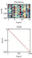
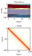
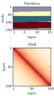
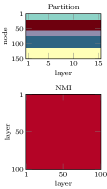
 , top) for a single example output partition and NMI values not (b) (0
  1, bottom) between induced partitions in different layers averaged over a sample of 10 output partitions. The parameter values match those in the numerical examples in Section VI (with the exception of , which we include for completeness). We choose a node ordering for each visualization that (whenever possible) emphasizes “persistent” mesoscale structure Bazzi et al. (2016). We show only the first layers of each multilayer partition, because (as one can see in the NMI heat maps) similarities between induced partitions for decay steeply with the number of layers when dependencies exist only between contiguous layers.
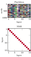
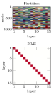
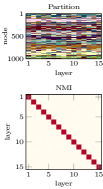
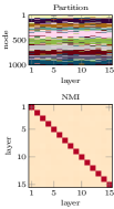
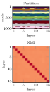
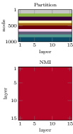
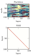
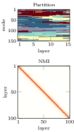
 , top) for a single example output partition and NMI
values not (b) (0
  1, bottom) between induced partitions in different layers averaged over a sample of 10 output partitions. (For the temporal case in Fig. 4, note that .) The parameter values match those in the numerical examples in Section VI (with the exception of , which we include for completeness). We choose a node ordering that (whenever possible) emphasizes “persistent” mesoscale structure Bazzi et al. (2016).
In Fig. 4 and Fig. 5, we show example multilayer partitions that we obtain with the interlayer-dependency tensors of Fig. 2. The examples in Fig. 4 are temporal, and the examples in Fig. 5 are multiplex. For simplicity, we assume in Fig. 2a that dependencies between contiguous layers are uniform (i.e., for all ). To illustrate the effect of the interlayer dependencies, we also show a heat map of the normalized mutual information (NMI) not (b) between induced partitions in different layers. NMI is a measure of similarity between partitions, so we expect the values of NMI to reflect the planted dependencies. As expected, for the temporal examples, partitions are most similar for adjacent layers. Similarities decay with the distance between layers and increase with the value of . For the multiplex examples, we obtain approximately uniform similarities between pairs of layers (for all pairs of layers), where the similarities increase with the value of . We use the examples of interlayer dependency of Figs. 4 and 5, as well as non-uniform and multi-aspect examples, in our numerical experiments of Section VI.
To provide a detailed illustration of the steps that result in a multilayer partition, we focus on the temporal examples in Fig. 4. For the important special case of temporal interlayer dependencies, the generative model for multilayer partitions simplifies significantly. In particular, there is a single ordered aspect, so the layer index is a scalar and the order of the layers corresponds to temporal ordering. Furthermore, as we mentioned in Section IV.2, for a fully-ordered multilayer network, we require that the order of the meso-set-assignment update process in Eq. 4 respects the order of the layers. The update order of state nodes in any given layer can be arbitrary (so we can update them simultaneously), but each update is conditional on the meso-set assignment of state nodes in layer .
The update process that we described in Section IV.2 reduces to three steps: (1) initialize (in an arbitrary order) the meso-set assignments in layer ; (2) take the meso-set assignment of to be that of with probability , and sample the meso-set assignment of from with complementary probability ; and (3) repeat steps (1) and (2) until . As we mentioned in Section IV.2, convergence is not an issue for this case (or, more generally, for any fully-ordered multilayer network), as we need only one iteration through the layers. This three-step generative model for temporal partitions was also suggested by Ghasemian et al Ghasemian et al. (2019). They used it to derive a detectability threshold for the case in which the null distributions are uniform across meso-sets (i.e., in Section IV.1) and intralayer edges are generated independently using the standard SBM. In other words, one replaces the degree-corrected SBM in Section V with the non-degree-corrected SBM of Holland et al. (1983). In Appendix C, we highlight properties of a sampled temporal partition that illustrate how the interplay between and the null distributions affects the evolution of meso-sets across layers (e.g., growth, birth, and death of induced meso-sets). The properties that we highlight hold for any choice of null distribution. In the same appendix, we subsequently illustrate that the particular choice of null distributions can greatly influence resulting partitions. For example, a non-empty overlap between the supports of null distributions that correspond to contiguous layers is a necessary condition for meso-sets to gain new state nodes over time. The properties and observations in Appendix C are independent of one’s choice of planted-partition network model.
V Generating network edges
There are diverse different types of multilayer networks Kivelä et al. (2014); Porter (2018). One common type of empirical multilayer network to study is one with only intralayer edges. There are also many empirical multilayer networks with both intralayer and interlayer edges (e.g., multimodal transportation networks Gallotti and Barthélemy (2014)), as well as ones with only interlayer edges (e.g., temporal networks with edge delays, such as departures and arrivals of flights between airports Boccaletti et al. (2014); Zanin and Lillo (2013)). One can use our framework to generate all three types of examples, provided the underlying edge generation model is a planted-partition network model.
Having generated a multilayer partition with dependencies between induced partitions in different layers, the simplest way to generate edges is to use any single-layer planted-partition network model (e.g., SBMs Karrer and Newman (2011); Holland et al. (1983); Jacobs and Clauset (2014); Peixoto (2018); Aicher et al. (2014); Galhotra et al. (2018), models for spatially-embedded networks Sarzynska et al. (2015); Newman and Peixoto (2015), and so on) and to generate edges for each layer independently. This yields a multilayer network with only intralayer edges, such that any dependencies between different layers result only from dependencies between the partitions that are induced on the different layers. For our numerical experiments in Section VI, we use a single-layer network model that is a slight variant (avoiding the creation of self-edges and multi-edges) of the degree-corrected SBM (DCSBM) benchmark from Karrer and Newman (2011), where “DCSBM benchmark” designates the specific type of DCSBM that was used in the numerical experiments of Karrer and Newman (2011). We include pseudocode for our implementation of the DCSBM benchmark in Algorithm 3 of Appendix D.
One can also include dependencies between layers other than those that are induced by planted mesoscale structures. For example, one can introduce dependencies between the parameters of a single-layer planted-partition network model by (1) sampling them from a common probability distribution (e.g., interlayer degree correlations Kivelä et al. (2014); Lee et al. (2012) in a DCSBM) or by (2) introducing interlayer edge correlations, given a single-layer partition on each layer Pamfil et al. (2019b). For temporal networks, one can also incorporate “burstiness” Holme and Saramäki (2012); Holme (2015); Lambiotte et al. (2013) in the inter-event-time distribution of edges. In such a scenario, the probability for an edge to exist in a given layer depends not only on the induced partition on that layer but also on the existence of the edge in previous layers. For example, one can use a Hawkes process to specify the time points at which edges are active Daley and Vere-Jones (2003); Hawkes (1971).
In Appendix D, we describe a generalization of the DCSBM in Karrer and Newman (2011) to multilayer networks that one can use to generate intralayer edges and/or interlayer edges. Our generalization constitutes a framework within which we formulate the parameters of a single-layer DCSBM in a multilayer setting. One can use our multilayer DCSBM (M-DCSBM) framework to incorporate some of the features that we described in the previous paragraph (e.g., degree correlations) in a multilayer network with intralayer and/or interlayer edges.
VI Numerical examples
In this section, we use our framework to construct benchmark models for multilayer community-detection methods and algorithms. We use the examples of interlayer-dependency tensors from Figs. 2 and 3 to generate benchmark models. We also consider a variant of Fig. 2b in which we split the layers into groups, use uniform dependencies between layers in the same groups, and treat layers in different groups as independent of each other. These examples cover commonly studied temporal and multiplex dependencies, and they illustrate how one can generate benchmark multilayer networks with more than one aspect. We focus on a couple of popular quality functions for multilayer community detection in our numerical examples, rather than investigating any given method or algorithm in detail.
We compare the behavior of several variants of Jeub et al. (2011–2019), which are similar to the the locally greedy Louvain computational heuristic Blondel et al. (2008), to optimize a multilayer modularity objective function Mucha et al. (2010); Bazzi et al. (2016) using the standard Newman–Girvan null model (which is a variant of a “configuration model” Fosdick et al. (2018)). Modularity is an objective function that is often used to partition sets of nodes into communities that have a larger total internal edge weight than the expected total internal edge weight in the same sets in a “null network” Bazzi et al. (2016), which is generated from some null model. Modularity maximization consists of finding a partition that maximizes this difference. For our numerical experiments, we use the generalization of modularity to multilayer networks of Mucha et al. (2010). For multilayer modularity, the strength of the interactions between different layers are governed by an interlayer-coupling tensor that controls the incentive for state nodes in different layers to be assigned to the same community. We use multilayer modularity with uniform interlayer coupling, so the strength of the interactions between different layers of the network depends on a layer-independent and node-independent interlayer coupling weight . We use diagonal and categorical (i.e., between all pairs of layers) interlayer coupling with weight for the multiplex examples in Section VI.1. We use diagonal and ordinal (i.e., between contiguous layers) interlayer coupling with weight for the temporal examples in Section VI.2. In Appendix E, we describe the Louvain algorithm and the variants of it that we use in this section.
We compare the results of multilayer modularity maximization with those of multilayer InfoMap 555We use version 0.18.2 of the InfoMap code with the “--two-level” option. The code is available at http://mapequation.org/code. Domenico et al. (2015), which uses an objective function called the “map equation” (which is not an equation), based on a discrete-time random walk and ideas from coding theory, to coarse-grain sets of nodes into communities Rosvall and Bergstrom (2007). In multilayer InfoMap, one uses a probability called the “relaxation rate” to control the relative frequency with which a random walker remains in the same layer or moves to other layers. (A random walker cannot change layers when .) The relaxation rate thus controls the interactions between different layers of a multilayer network. We allow the random walker to move to all other layers when for the multiplex examples in Section VI.1, and we allow the random walker to move only to adjacent layers for the temporal examples in Section VI.2. In contrast to multilayer modularity (where yields single-layer modularity), single-layer InfoMap is not equivalent to choosing in multilayer InfoMap because placing state nodes that correspond to the same physical node in the same community can contribute positively to the quality function even when Domenico et al. (2015). Consequently, we compute single-layer InfoMap separately and reference it by the data point “s” on the horizontal axis.
In all experiments in this section, we generate a multilayer partition using our copying process in Section IV (see Algorithm 1 in Appendix B) and a multilayer network for a fixed planted partition using a slight variant of the DCSBM benchmark network model in Karrer and Newman (2011) that avoids generating self-edges and multi-edges (see Algorithm 3 in Appendix D). This produces multilayer networks that have only intralayer edges and in which the connectivity patterns in different layers depend on each other. Following Karrer and Newman (2011), we parametrize the DCSBM benchmark in terms of its distribution of expected degrees and a community-mixing parameter that controls the strength of the community structure in the sampled network edges. For , all edges lie within communities; for , edges are distributed independently of the communities, where the probability of observing an edge between two state nodes in the same layer depends only on the expected degrees of those two state nodes. We use a truncated power law for the distribution of expected degrees.
The DCSBM benchmark imposes community structure as an expected feature of an ensemble of networks that it generates. The definition of the mixing parameter of the DCSBM benchmark ensures that the planted partition remains community-like — as intra-community edges are more likely to be observed and inter-community edges are less likely to be observed than in a network that is generated from a single-block DCSBM with the same expected degrees — for any value of . Consequently, given sufficiently many samples from the same DCSBM benchmark (i.e., all samples have the same planted partition and same expected degrees), one should be able to identify the planted community structure for any value of (where the necessary number of samples goes to infinity as ). This feature makes the DCSBM benchmark an interesting test for the ability of multilayer community-detection methods to aggregate information from multiple layers.
We use NMI not (b) to compare the performance of different community-detection algorithms. For each of our partitions, we compute the mean of the NMI between the partition induced on each layer by the output partition and that induced by the planted partition. That is,
The quantity is invariant under permutations of the meso-set labels within a layer. Consequently, is well-suited to comparing multilayer community-detection methods with single-layer community-detection methods. In particular, it allows us to test whether multilayer community-detection methods can exploit dependencies between layers of a multilayer network when (see Eq. 6). In Appendix F, we show numerical experiments in which we compute NMI between multilayer partitions. We denote the NMI between two multilayer partitions by mNMI.
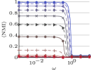
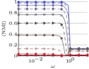
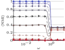
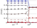
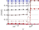
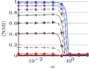
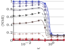
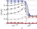
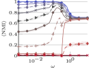
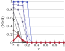
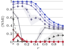
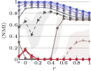
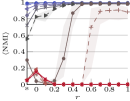
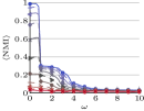
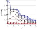
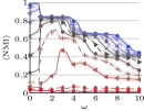
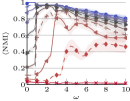
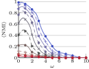
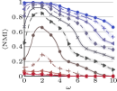
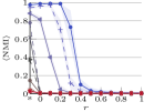
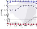
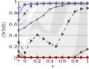
In all of our numerical experiments in Sections VI.1 and VI.2, we sample the benchmark networks in the following way. For each value of , we generate sample partitions. For each sample partition and value of , we generate sample multilayer networks. This yields benchmark instantiations for each pair . We run each community-detection algorithm times on each instantiation. In Figs. 6, 8, 7, and 9, we show between planted and recovered multilayer partitions averaged over sample partitions, sample networks, and algorithmic runs for each value of . The results for different planted partitions are generally similar. The only exception is InfoMap on temporal networks with and , where we observe large differences between results for different partitions for certain values of .
Figures 6, 8, 7, and 9 correspond to different choices for the interlayer-dependency tensor. In each figure, rows correspond to different choices for the community-detection algorithm, and columns correspond to different values of the copying probabilities (with the strength of interlayer dependencies increasing from left to right). All benchmark instantiations that we use for Figs. 6, 8, 7, 9, and 10 are available at https://dx.doi.org/10.5281/zenodo.3304059.
| GenLouvain |
|---|
 (a)
(a)
 (b)
(b)
 (c)
(c)
 (d)
(d)
 (e)
(e)
|
| GenLouvainRand |
 (f)
(f)
 (g)
(g)
 (h)
(h)
 (i)
(i)
 (j)
(j)
|
| InfoMap |
 (k)
(k)
 (l)
(l)
 (m)
(m)
 (n)
(n)
 (o)
(o)
|
VI.1 Multiplex examples
| GenLouvain |
|---|
|
|
| GenLouvainRand |
|
|
| InfoMap |
|
|
In this section, we consider two stylized examples of multiplex networks. Multiplex networks arise in a variety of different applications, including international relations and trade Cranmer et al. (2015); Barigozzi et al. (2010); Mastrandrea et al. (2014), social networks Fan and Yeung (2015), and ecological networks Kéfi et al. (2016). In our multiplex examples, we consider simple dependency structures in which we expect multilayer community-detection methods to outperform single-layer methods by exploiting interlayer dependencies.
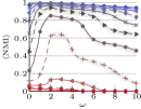
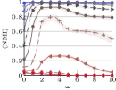
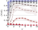
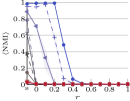
In Fig. 6, we consider multiplex networks with uniform dependencies between community structure in different layers. In Fig. 7, we consider multiplex networks with nonuniform dependencies between community structure in different layers. In both figures, we parametrize the amount of interlayer dependency in a network by the probability (see Eq. 6) that a state node copies its community assignment from a neighbor in the interlayer-dependency network. All multilayer networks have physical nodes and layers. Each node is present in every layer, so there are a total of state nodes. In Fig. 2b, we show the layer-coupled interlayer-dependency matrix that we use to generate the uniform multiplex networks. For the nonuniform multiplex networks, we split the layers into groups of layers each. We use uniform dependencies between layers in the same group, and layers in different groups are independent of each other. The resulting layer-coupled interlayer-dependency matrix is block diagonal with diagonal blocks as in Fig. 2b and entries on the off-diagonal blocks. We use a Dirichlet null distribution with , , and (see Appendix A) to specify expected community sizes and the M-DCSBM benchmark (see Appendix D) with , , and to generate intralayer edges. We perform iterations of our update process (see Appendix B).
Comparing our results for GenLouvain (Figs. 6a, 6b, 6c, 6d, 6e, 7a, 7b, and 7c) and GenLouvainRand with reiteration and post-processing (Figs. 6f, 6g, 6h, 6i, 6j, 7d, 7e, and 7f), we see that the choice of optimization heuristic for a given quality function can significantly affect the quality of resulting identified partitions. In particular, for GenLouvain, we observe two distinct regimes and what appears to be a sharp transition between them 666We observe some erratic behavior at the transition as the interlayer coupling approaches from below. For values of near but smaller than , the GenLouvain algorithm has a tendency to place all state nodes in a single community. This observation is related to the transition behavior that was described in Bazzi et al. (2016). For values of above a certain threshold Bazzi et al. (2016) only interlayer merges occur in the first phase of Louvain.. For , we obtain a partition that is of similar quality to what we obtain by maximizing single-layer modularity; however, for , we obtain a partition with identical induced partitions for each layer. We call the latter an aggregate partition. Although the aggregate partition can be more similar to the planted partition than the single-layer partition when is sufficiently large (e.g., this occurs in Figs. 6d and 6e), we do not observe an interval of values between the two regimes in which GenLouvain recovers the planted partition better than both the single-layer and aggregate partitions. By contrast, GenLouvainRand with reiteration and post-processing identifies partitions that match the planted partition more closely than either the single-layer or aggregate partitions in most cases. The exceptions are uniform multiplex networks with (see Fig. 6f), where it is unable to exploit the weak dependencies to outperform the single-layer case; and (Fig. 6j), where the aggregate partition is always best. Most of the improvement in the results for GenLouvainRand over those for GenLouvain comes from reiteration. The additional randomization helps smooth out the transition at . Post-processing only yields a minor improvement in the value of . However, its effect is more pronounced if we compute the mNMI between multilayer partitions (see Appendix F).
Multilayer InfoMap exhibits some problematic behavior in these benchmark experiments. Our results for multilayer InfoMap are noticeably worse than those that we obtain with single-layer InfoMap (corresponding to the data point “s” on the horizontal axis) for networks with comparatively weak community structure (specifically, ), unless the planted partition for different layers is very similar (i.e., unless ). Furthermore, the methods that are based on multilayer modularity outperform multilayer InfoMap in our experiments for networks with weak community structure and similar layers (i.e., when both and are close to ). InfoMap does not identify meaningful community structure in networks with in any of our numerical examples, whereas GenLouvain and GenLouvainRand identify meaningful structure even for networks with very weak community structure (e.g., with ) for sufficiently large values of .
| GenLouvain |
|---|
 (a)
(a)
 (b)
(b)
 (c)
(c)
 (d)
(d)
 (e)
(e)
|
| GenLouvainRand |
 (f)
(f)
 (g)
(g)
 (h)
(h)
 (i)
(i)
 (j)
(j)
|
| InfoMap |
 (k)
(k)
 (l)
(l)
 (m)
(m)
 (n)
(n)
 (o)
(o)
|
Our results for nonuniform multiplex networks in Fig. 7 are similar to those that we showed for the uniform multiplex networks in Fig. 6. In particular, we see that GenLouvainRand can exploit dependencies between community structure in different layers (although the improvement over single-layer modularity is less pronounced than in the uniform examples), whereas GenLouvain cannot. The main difference is that for , the aggregate partitions from GenLouvain and GenLouvainRand do not recover the planted partition for sufficiently large values of , because the induced partitions are not identical across layers in the planted partition. In principle, multilayer InfoMap should have an advantage over methods based on maximizing multilayer modularity in this case study, as the former’s quality function is designed to detect breaks in community structure, whereas multilayer modularity forces some persistence of community labels between any pair of layers. In practice, however, multilayer InfoMap correctly identifies the planted community structure only when it is particularly strong (as we show in Appendix F, it correctly identifies the different groups of layers for networks with ); and it is outperformed by single-layer InfoMap for networks with .
We suspect that at least some of the shortcomings of multilayer InfoMap in these experiments are due to the use of a Louvain-like optimization heuristic, rather than from flaws in InfoMap’s quality function. As we have seen from the results with the heuristics GenLouvain and GenLouvainRand, seemingly minor adjustments of an optimization heuristic can have large effects on the quality of the results. We are thus hopeful that similar adjustments can also improve the results for multilayer InfoMap.
VI.2 Temporal examples
| GenLouvain |
|---|
|
|
| GenLouvainRand |
|
|
| InfoMap |
|
|
Temporal networks arise in many different applications Holme and Saramäki (2012); Holme (2015), such as the study of brain dynamics Betzel and Bassett (2017), financial-asset correlations Bazzi et al. (2016), and scientific citations Hric et al. (2018). When representing a temporal network as a multilayer network, one orders the layers in a causal way, such that structure in a particular layer depends directly only on structure in previous layers (and not in future layers). To generate multilayer networks that have such structure, we use our sampling process for fully-ordered multilayer networks and the interlayer-dependency tensor of Fig. 2a.
We consider two stylized examples of temporal networks. In Fig. 8, we show results for temporal networks that have uniform dependencies between consecutive layers (and hence tend to evolve gradually). To generate these networks, we set for all layers in Fig. 2a. In Fig. 9, we show results for temporal networks with change points. To generate these networks, we set for all layers except layers 25, 50, and 75, for which , resulting in abrupt changes in community structure. Each multilayer network in these two examples has physical nodes and layers. Each node is present in every layer, so there are a total of state nodes. We use a Dirichlet null distribution to specify expected community sizes and set , , and (see Appendix A). For the temporal networks with change points in Fig. 9, we choose the support of the null distribution so that communities after a change point have new labels. We use the M-DCSBM benchmark (see Appendix D) with , , and to generate intralayer edges.
Both multilayer-modularity-based algorithms (i.e., GenLouvain and GenLouvainRand) can exploit interlayer dependencies for these temporal benchmark networks and identify partitions with significantly larger than those that we obtain with single-layer modularity (i.e., with ). Typically, the peak of seems to occur when . When , one expects to decrease for sufficiently large values of , as increasing further favors “persistence” Bazzi et al. (2016) in the output partition that is not present in the multilayer planted partition.
For multilayer InfoMap, the results are less promising. For most parameter choices, the best result for multilayer InfoMap is at best similar and often worse than the result for single-layer InfoMap. (The value for single-layer InfoMap is the data point that we label with “s” on the horizontal axis.) An exception are the results for and uniform temporal dependencies (see Fig. 8o). In this example (where induced partitions are the same across layers), increasing the value of the relaxation rate enhances the recovery for all sampled planted partitions when and for a subset of sampled planted partitions when and . The results for multilayer InfoMap on temporal benchmarks with uniform interlayer dependencies with (see Fig. 8n for and ) and (see Fig. 8o for and ) are the only instances where we observe large differences in results for different partitions that are generated by our model with the same parameter values.
Comparing results for GenLouvain (see Figs. 8a, 8b, 8c, 8d, 8e, 9a, 9b, and 9c) and GenLouvainRand with reiteration and post-processing (see Figs. 8f, 8g, 8h, 8i, 8j, 9d, 9e, and 9f), we see that the difference in results between the two optimization heuristics for multilayer modularity is even more pronounced in these temporal examples than in the multiplex examples in Section VI.1. In particular, GenLouvain exhibits an abrupt change in behavior near ; this is related to the transition behavior that was described in Bazzi et al. (2016). As we explained in Section VI.1 (where we also observed this phenomenon), this transition occurs for the following reason: for values of that are above a certain threshold Bazzi et al. (2016), only interlayer merges occur in the first phase of the Louvain heuristic. This abrupt transition no longer occurs with the additional randomization in GenLouvainRand, which exhibits smooth behavior as a function of . However, unlike in our multiplex experiments, we observe benefits from the behavior of GenLouvain in some situations, especially for networks with weak community structure (specifically, for ). This phenomenon first becomes noticeable for networks with , and it becomes more pronounced for progressively larger values of . Compare Figs. 8c, 8d, and 8e with Figs. 8h, 8i, and 8j; and compare Figs. 9b and 9c with Figs. 9e and 9f.
Our results for temporal benchmark networks with change points (see Fig. 9) are mostly similar to those for temporal benchmark networks with uniform dependencies when considering to compare planted and recovered partitions. Only the results for are noticeably different. (Compare Figs. 9c, 9f, and 9i with Figs. 8e, 8j, and 8o.) Because of the change points, the induced planted partitions for each layer are not identical, even when . Consequently, unlike in Fig. 8, the results for in Fig. 9 are qualitatively similar to those for smaller values of . In principle, one might expect multilayer InfoMap to have an advantage over multilayer-modularity-based methods in this experiment, as the former’s quality function is designed to detect abrupt changes in community structure, whereas maximizing multilayer modularity always favors some persistence of community labels from one layer to the next. However, this theoretical advantage is not borne out in our experiment. When comparing the planted and recovered partitions using the NMI between multilayer partitions, we see that multilayer InfoMap can correctly recover the change points only for and (see Appendix F).
VI.3 Multi-aspect examples
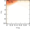
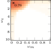
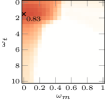
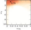
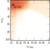
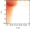
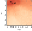
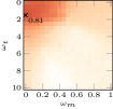
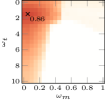
In this section, we illustrate the ability of our framework to generate multilayer networks with more than one aspect. A common situation that gives rise to multilayer networks with two aspects is a multiplex network that changes over time (e.g., citations patterns that change over time Starnini et al. (2017)). In our framework, such a situation corresponds to the interlayer-dependency tensor in Fig. 3. For the illustrative examples in this section, we use uniform multiplex and temporal dependencies; and we parametrize the interlayer dependency tensor as follows:
where controls the balance between multiplex and temporal dependencies and controls the overall strength of the interlayer dependencies.
To recover communities, we optimize a multi-aspect generalization,
| (8) | ||||
of the multilayer modularity function that was introduced in Mucha et al. (2010).
We specify the interlayer-coupling tensor (a multi-aspect generalization of the “interslice coupling” of Mucha et al. (2010)), such that it reflects the planted interlayer dependencies, by writing
where denotes the coupling parameter for the temporal dependencies and denotes the coupling parameter for the multiplex dependencies.
In Fig. 10, we illustrate the effects of the two interlayer coupling parameters, and , on the extent to which multilayer modularity maximization can recover a planted partition. We use GenLouvainRand with reiteration but without post-processing to find a local optimum of Eq. 8. For all of the values of and that we consider in Fig. 10, we see some improvement in the performance of multilayer modularity maximization with nonzero interlayer coupling compared with the case where both and . As the latter case corresponds to independently maximizing modularity on each layer of a network, this demonstrates that multilayer modularity is able to exploit the interlayer dependencies to better recover the planted partition. As expected, increasing (which gives more weight to temporal dependencies) leads to a shift of the region of the parameter space with good planted-partition recovery to larger values of and smaller values of . For progressively larger , we observe a small overall increase in the value of , but its dependence on and remains similar.
VII Conclusions
We introduced a unifying and flexible framework for the construction of generative models for mesoscale structures in multilayer networks. The three most important features of our framework are the following: (1) it includes an explicitly parametrizable tensor that controls interlayer-dependency structure; (2) it can generate an extremely general, diverse set of multilayer networks (including, e.g., temporal, multiplex, “multilevel” Lomi et al. (2016), and multi-aspect multilayer networks with uniform or nonuniform dependencies between state nodes); and (3) it is modular, as the process of generating a partition is separate from the process of generating edges, enabling a user to first generate a partition and then use any planted-partition network model. Along with our paper, we provide publicly available code Jeub and Bazzi (2016–2019) that users can modify to readily incorporate different types of null distributions (see Section IV.1), interlayer-dependency structures (see Section IV.2), and planted-partition network models (see Section V).
The ability to explicitly specify interlayer-dependency structure makes it possible for a user to control which layers depend directly on each other (by deciding which entries in the interlayer-dependency tensor are nonzero) and the strengths of such dependencies (by varying the magnitude of entries in the interlayer-dependency tensor). One can thereby generate multilayer networks with either a single aspect or multiple aspects (e.g., temporal and/or multiplex networks) and vary dependencies between layers from the extreme case in which induced partitions in a planted multilayer partition are the same across layers to the opposite extreme, in which induced partitions in a planted multilayer partition are generated independently for each layer from a null distribution for that layer. To the best of our knowledge, this level of generality is absent from existing generative models for mesoscale structures in multilayer networks, as those models tend to only consider networks with a single aspect (e.g., temporal or multiplex) or limited interlayer-dependency structures (e.g., with the same induced partitions in a planted multilayer partition across all layers).
We illustrated several examples of generative models that one can construct from our framework, with a focus on a few special cases of interest, rather than on trying to discuss as many situations as possible. We focused on community structure in our numerical experiments, because it is a commonly studied mesoscale structure, but one can also use our framework to construct generative models of intra-layer mesoscale structures other than community structure (e.g., core–periphery structure, bipartite structure, and so on) by taking advantage of the flexibility of our framework’s ability to use any single-layer planted-partition network model. For our single-aspect examples, we assumed that interlayer dependencies exist either between all contiguous layers (a special case of temporal networks), between all layers (a special case of multiplex networks), or between all contiguous groups of layers (another special case of multiplex networks). For both our temporal and multiplex examples, we considered both uniform and nonuniform interlayer dependencies. We also combined some of these scenarios in an example with two aspects, a temporal aspect and a multiplex aspect. However, our framework’s flexibility allows us to construct generative models of multilayer networks with more realistic features. For example, for temporal networks, one can introduce dependencies between a layer and all layers that follow it (such that Fig. 2a is an upper triangular matrix with nonzero entries above the diagonal) to incorporate memory effects Rosvall et al. (2014). One can also consider interlayer dependencies that are not layer-coupled. For example, dependencies can be diagonal but nonuniform, or they can be nonuniform and exist only between sets of related nodes.
In Section VI, we consider the commonly studied case of a multilayer network with only intralayer edges and connectivity patterns in the different layers that depend on each other. We use a slight variant of the DCSBM benchmark from Karrer and Newman (2011) to generate edges for each layer (see Algorithm 3). However, other types of multilayer networks are also important Kivelä et al. (2014), and one can readily combine our approach for generating multilayer partitions with different network generative models that capture various important features. For example, one can use an SBM to generate interlayer edges (e.g., using our M-DCSBM framework, which we discuss in Appendix D), or one can replace the degree-corrected SBM in Section V with any other planted-partition network model or other interesting models (e.g., other variants of SBMs Holland et al. (1983); Jacobs and Clauset (2014) and models for networks whose structure is affected by space (and perhaps spatially embedded) Sarzynska et al. (2015) or arbitrary latent features Newman and Peixoto (2015)). In all of these examples, dependencies between connectivity patterns in different layers arise only from a planted multilayer partition. It is also possible to modify our network generation process (see Section V) to incorporate additional dependencies between layers beyond those that are induced by a planted mesoscale structure, such as by introducing dependencies between a node’s degree in different layers Nicosia and Latora (2015); Lee et al. (2012) or burstiness Lambiotte et al. (2013) in inter-event-time distributions of edges.
Our work has the potential for many useful and interesting extensions, and we highlight three of these. First, although we have given some illustrative numerical examples in Section VI, the area of benchmarking community-detection methods in multilayer networks is far from fully developed. Generative models are useful tools for understanding the behavior of community-detection methods in detail and thus for suggesting ways of improving heuristic algorithms without losing scalability. One can use our framework to construct benchmark models that provide a test bed for gaining insight into the advantages and shortcomings of community-detection methods and algorithms (and, more generally, of meso-set-detection methods and algorithms). Importantly, we expect these benchmark models to be very informative for detecting potential artifacts of algorithms that can sometimes be masked in real-world applications. Second, a well-understood generative model can be a powerful tool for statistical inference (i.e., inferring the structure of a multilayer network rather than generating a multilayer network with a planted structure) Fortunato and Hric (2016). For temporal networks, closed forms for the joint distribution of meso-set assignments have been derived for models that are special cases of our framework Ghasemian et al. (2016); Pamfil et al. (2019a). These results may be useful for statistical inference. Additionally, it seems likely that it is possible to adapt Bayesian inference techniques (including Gibbs sampling Snijders and Nowicki (1997); Nowicki and Snijders (2001); Peixoto (2017) or variational methods Latouche et al. (2012)) that have been developed for SBMs both for inferring a multilayer partition and for inferring an interlayer-dependency tensor. A key advantage of the generality of the framework that we have developed in the present paper is that it may be possible to frame many model-selection questions in terms of posterior estimation of the interlayer-dependency tensor. Finally, it is important to model interdependent data streams and not just fixed data sets. For example, for any fully-ordered multilayer network, our generative model respects the causality of layers (e.g., temporal causality), and one can thus update a multilayer network with a new layer without the need to update any previous layers. It is critical to develop generative models that are readily adaptable to such situations, and our work in this paper is a step in this direction.
Appendix A Example null distributions
In this appendix, we discuss parameter choices for a categorical null distribution and give concrete examples that can be useful for modeling mesoscale structure in temporal or multiplex networks.
In Section IV.1, we described the general form of a categorical null distribution:
| (9) |
where is the probability for a state node in layer to be assigned to a meso-set in the absence of interlayer dependencies, is the number of meso-sets in the multilayer partition, and for each . The support of the null distribution is . We say that a label is active in a layer if it is in the support of the null distribution (i.e., if ); and we say that a label is inactive in layer if it is in the complement of the support of (i.e., if ).
A natural choice is to sample from a Dirichlet distribution, which is the conjugate prior for the categorical distribution Raiffa and Schlaifer (2000); Agarwal and Daumé III (2010). The Dirichlet distribution over variables has parameters . Its probability density function is
where and for each . The case in which all are equal is called a “symmetric Dirichlet distribution”, which we parametrize by the common value (the so-called “concentration parameter”) of the parameters and the number of variables.
The concentration parameter determines the types of discrete probability distributions that one is likely to obtain from the symmetric Dirichlet distribution. For , the symmetric Dirichlet distribution is the continuous uniform distribution over the space of all discrete probability distributions with states. As , the Dirichlet distribution becomes increasingly concentrated near the discrete uniform distribution, such that all entries in are approximately equal. As , it becomes increasingly concentrated away from the uniform distribution, such that tends to have (or a few) large entries and all other entries are close to . Consequently, to have very heterogeneous meso-set sizes, one would choose . To have all meso-sets be of similar sizes, one would choose a large value of . To have a few large meso-sets and many small meso-sets, one would choose to be sufficiently smaller than . The value of also affects the amount of meso-set label overlap across layers in the absence of interlayer dependencies. For example, if is the same for all layers, then larger values of incentivize less label overlap across layers (because there are more possible labels for each layer) and smaller values of incentivize more label overlap across layers (because there are fewer possible labels for each layer).
In some situations — e.g., when modeling the birth and death of communities in temporal networks or the appearance and disappearance of communities in multiplex networks — it is desirable to have meso-set labels that have a nonzero probability in (9) only in some layers. For these situations, we suggest sampling the support of the distributions before sampling the probabilities . Given the supports for each layer, one then samples the corresponding probabilities from a symmetric Dirichlet distribution (or any other distribution over categorical distributions). That is,
| (10) |
where is the complement of the support, with .
A simple example for a birth/death process for meso-sets is the following. First, fix a number of meso-sets and a support (i.e., active community labels) for the first layer. One then sequentially initializes the supports for the other layers by removing each meso-set in the support of the previous layer with probability and adding a number, sampled from a Poisson distribution with rate , of new meso-sets (with new labels that are not active in any previous layer). In temporal networks, for example, this ensures that if a meso-set label is not in the support of a given layer, then the label is also not in the support of any subsequent layers. For this process, the expected number of meso-sets in a layer approaches as one iterates through the layers. Therefore, one should initialize the size of the support for the first layer close to this value to avoid transients in the number of meso-sets. For this process, the lifetime of meso-sets follows a geometric distribution. The nature of the copying process that we use to introduce dependencies between induced partitions in different layers typically implies that meso-sets that have been removed from the support of the null distribution do not lose all of their members instantly, but instead shrink at a speed that depends on the values of the copying probabilities in the interlayer-dependency tensor.
One can also allow labels to appear and disappear when examining multiplex partitions. For example, given a value for , one can generate the support for each layer by allowing each label to be present with some probability and absent with complementary probability . This yields a sets of active and inactive meso-set labels for each layer. One can then sample the nonzero probabilities in that correspond to active labels from a Dirichlet distribution and set to for each inactive label . Because multiplex partitions are unordered, there is no notion of one layer occurring after another one, so we do not need to ensure that an inactive label in a given layer is also inactive in “subsequent” layers.
Appendix B Partition sampling process
In this appendix, we provide a detailed description of the way in which we sample multilayer partitions, including a discussion of the convergence properties of our sampling process. As we mentioned in Section IV.2, we assume that the multilayer partitions are generated by a copying process on the meso-set assignment of state nodes. Recall that the conditional probability distribution for the updated meso-set assignment of a state node, given the current state of the copying process (Eq. 4 in Section IV.2), is
| (11) | ||||
where is a given set of independent layer-specific null distributions and is a given interlayer-dependency tensor. Further recall that a multilayer network can have both ordered aspects and unordered aspects, where we denote the set of ordered aspects by and the set of unordered aspects by . Our goal is to sample multilayer partitions that are consistent with generation by Eq. 11 while respecting the update order from its ordered aspects (if present). Recall that two layers, and , are order-equivalent (which we denote by ) if for all . Based on this equivalence relation, we obtain an ordered set of equivalence classes by inheriting the order from the ordered aspects (where, for definiteness, we consider the lexicographic order not (a) over ordered aspects). We want to simultaneously sample the meso-set assignment of state nodes within each class of order-equivalent layers and we want to sequentially sample the meso-set assignment of state nodes in non-order-equivalent layers, conditional on the fixed assignment of state nodes in preceding layers (see Algorithm 1).
Scan order and compatibility
To sample the induced partitions for each class of order-equivalent layers, we use a technique that resembles Gibbs sampling Gelfand (2000). As in Gibbs sampling, we define a Markov chain on the space of multilayer partitions by updating the meso-set assignment of state nodes by sampling from Eq. 11. In Gibbs sampling, one assumes that the conditional distributions that are used to define this Markov chain are compatible, in the sense that there exists a joint distribution that realizes these conditional distributions Hobert and Casella (1998); Arnold and Press (1989); Chen (2010); Chen and lp (2015). However, for a general interlayer-dependency tensor, there is no guarantee that the distributions that are defined by Eq. 11 are compatible. Following Heckerman et al. (2000), we use the term “pseudo-Gibbs sampling” to refer to Gibbs sampling from a set of potentially incompatible conditional distributions. We can define different Markov chains by changing the way in which we select which conditional distribution to apply at each step (i.e., which state node to update at each step). The order in which one cycles through the conditional distributions is known as the scan order Kuo and Wang (2017). We use the term sampling Markov chain for the Markov chain that is defined by pseudo-Gibbs sampling with a specified scan order. Common scan orders are cycling through conditional distributions in a fixed order and sampling the update distribution uniformly at random from the set of conditional distributions. In pseudo-Gibbs sampling, the choice of scan order deserves careful attention. In pseudo-Gibbs sampling, different scan orders correspond to sampling from different distributions Kuo and Wang (2017). (By contrast, in Gibbs sampling, the choice of scan order influences only the speed of convergence.) In particular, when cycling through conditional distributions in a fixed order, conditional distributions that are applied later have an outsized influence on the stationary distributions of the sampling Markov chain Kuo and Wang (2017). Sampling the update distribution uniformly at random mitigates this problem, at the expense of introducing computational overhead.
We can improve on a purely random sampling strategy by exploiting the structure of the interlayer-dependency tensor. In particular, note that the conditional distributions for state nodes in the same layer are independent (as we assume that the interlayer-dependency tensor has no intralayer contributions) and hence compatible. When updating a set of state nodes from a given layer, we can update them in any order or even update them concurrently. To take advantage of this fact, we first sample a layer uniformly at random from the current class of order-equivalent layers and then update all state nodes in that layer. The sequence of layer updates defines a Markov chain on the space of multilayer partitions, and its convergence properties determine the level of effectiveness of our sampling algorithm.
Convergence guarantees
We now discuss two key properties — aperiodicity and ergodicity — that determine the convergence behavior of finite Markov chains.
First, note that sampling layers uniformly at random guarantees that the Markov chain is aperiodic. To see this, note that a sufficient condition for aperiodicity is that, for all states, there is a nonzero probability to transition from the state to itself. This clearly holds for our sampling chain, as it is possible for two consecutive updates to update the same layer, and (because the probability distributions in Eq. 11 remain unchanged at the second update) there is a positive probability that the second update does not change the partition.
Second, note that if for all state nodes such that , where is a class of order-equivalent layers, then the sampling Markov chain for that class is ergodic over a subspace of multilayer partitions that includes the support of the null distributions. We have already shown that the sampling Markov chain is aperiodic, so all that remains is to verify that there exists a sample path from any arbitrary initial partition to any arbitrary multilayer partition in the support of the null distributions. Such a sample path clearly exists, as
Therefore, one can achieve the desired transition using one update for each state node.
Sample paths of a finite, aperiodic Markov chain converge in distribution to a stationary distribution of the Markov chain. However, different sample paths can converge to different distributions, and the eventual stationary distribution can depend both on the initial condition and on the transient behavior of the sample path. If the Markov chain is ergodic, the stationary distribution is unique, so it is independent of the initial condition and transient behavior.
After sufficiently many updates (i.e., by specifying a sufficiently large value for the expected number of updates for each state node in Algorithm 1), we approximately sample the state of the Markov chains for each class of order-equivalent layers from their stationary distributions. For fully-ordered multilayer networks (i.e., for multilayer networks with ), setting is sufficient for convergence, because the equivalence classes include only a single layer in this case and subsequent updates are thus independent samples from the same distribution.
Sampling initial conditions in an ‘unbiased’ way can be important for ensuring that one successfully explores the space of possible partitions, as the updating process is not necessarily ergodic over the support of the null distributions when for some state nodes. For example, if for all , then any partition in which all state nodes in each weakly connected component of the interlayer-dependency network have the same meso-set assignment is an absorbing state of the Markov chain.
However, provided the updating process has converged, any partition that one generates should still reflect the desired dependencies between induced partitions for different layers. Therefore, to circumvent the problem of non-unique stationary distributions when the updating process is not ergodic, we reinitialize the updating process by sampling from the null distribution for each partition that we want to generate. Reinitializing the initial partition from a fixed distribution for each sample always defines a unique joint distribution, which is a mixture of all possible stationary distributions when the updating process is not ergodic. When the updating process is ergodic, it is equivalent to sample partitions by reinitializing or to sample multiple partitions from a single long chain. Using a single long chain is usually more efficient when one needs many samples and it is not problematic if there is some dependence between samples Tierney (1994). In our case, however, we usually need only a few samples with the same parameters, and ensuring independence tends to be more important than ensuring perfect convergence (provided the generated partitions exhibit the desired interlayer-dependency structure). Using multiple chains thus has clear advantages even when the updating process is ergodic, and it is necessary to use multiple chains when it is not ergodic.
Convergence tests

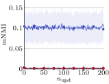
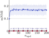
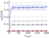
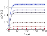


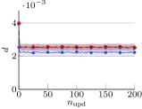
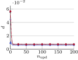
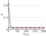
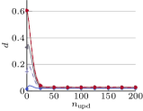
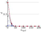
It is difficult to determine whether a Markov chain has converged to a stationary distribution, mostly because it is difficult to distinguish the case of a slow-mixing chain becoming stuck in a particular part of state space from the case in which the chain has converged to a stationary distribution. There has been much work on trying to define convergence criteria for Markov chains Cowles and Carlin (1996), but none of the available approaches are entirely successful. In practice, one usually runs a Markov chain (or chains) for a predetermined number of steps. One checks manually for a few examples that the resulting chains exhibit behavior that is consistent with convergence by examining autocorrelations between samples of the same chain and cross-correlations between samples of independent chains with the same initial state. When feasible, one can also check whether parts of different, independent chains or different parts of the same chain are consistent with sampling from the same distribution.
To estimate the number of updates that we need in the numerical experiments of Section VI.1, we examine the autocorrelation of the Markov chain in two different ways. In Fig. 11, we consider the multilayer NMI (mNMI) between sampled partitions at different steps of the Markov chain. We are interested in the behavior of the mNMI both as a function of (the expected number of updates per state node that we use to generate the first partition in the comparison) and the lag (the number of additional updates per state node that we use to generate the second partition in the comparison). As the Markov chain converges to a stationary distribution, the value of the mNMI for a given lag should become independent of (so the curves in Fig. 11 should become flat). The results in Fig. 11 suggest that the number of updates that we need for convergence increases moderately with , where is sufficient for convergence even when . In Fig. 12, we examine whether the dependency pattern between induced partitions in different layers — we characterize such a pattern by the NMI between induced partitions in different layers — has converged using the mean absolute distance
| (12) |
between the NMI matrices between induced partitions in a multilayer partition. (We showed examples of such NMI matrices in Figs. 4 and 5.) As with mNMI, the mean absolute distance should become independent of once the Markov chain has converged to a stationary distribution. This yields estimates for the minimum number of updates for convergence that are consistent with those from the results in Fig. 11. It is always safe to use a larger number of updates to sample partitions, and the results from Figs. 12 and 11 suggest that our choice of is conservative.
Figures 11 and 12 reveal additional important information about the behavior of our sampling process. We can estimate the mixing time of the sampling Markov chain at stationarity from Fig. 11, because the mixing time corresponds to the lag that is necessary for the mNMI to converge to . The mixing time at stationarity increases with and becomes infinite as , because the Markov chain converges to an absorbing state. From Fig. 12, we observe that, for all values of , the mean absolute distance between NMI matrices converges to a value near and becomes essentially independent of the lag. This corroborates our assumption that different partitions that we generate from our sampling process have similar interlayer-dependency structure.
Appendix C A generative model for temporal networks
In this appendix, we examine the generative model for temporal networks that we considered in Section IV.4. In this model, we assume uniform dependencies between contiguous layers (i.e., for all in Fig. 2a). For this choice of interlayer-dependency tensor, our generative model reduces to Algorithm 2. In this case (and, more generally, for any fully-ordered multilayer network), convergence is automatic, because we need only one iteration through the layers.
A first important feature of the generative model in Algorithm 2 is that it respects the arrow of time. In particular, meso-set assignments in a given layer depend only on meso-set assignments in the previous layer (e.g., the previous temporal snapshot) and on the null distributions . That is, for all and all , we have
| (13) | ||||
where is the -node partition that is induced on layer by the multilayer partition . The value of determines the relative importance of the previous layer and the null distribution. When , meso-set assignments in a given layer depend only on the null distribution of that layer (i.e., on the second term of the right-hand side of Eq. 13). When , meso-set assignments in a given layer are identical to those of the previous layer (and, by recursion, to meso-set assignments in all previous layers).
Using Eq. 13, we see that the marginal probability that a given state node has a specific meso-set assignment is
Computing marginal probabilities can be useful for computing expected meso-set sizes for a given choice of null distributions.
We now highlight how the copying update (i.e., Step C) and the reallocation update (i.e., Step R) in Algorithm 2 govern the evolution of meso-set assignments between consecutive layers. Steps C and R deal with the movement of nodes by first removing some nodes (“subtraction”) and then reallocating them (“addition”). In Step C, a meso-set assignment in layer can lose a number of nodes that ranges from to all of them. It can keep all of its nodes in layer (i.e., ), lose some of its nodes (i.e., ), or disappear entirely (i.e., and ). The null distribution in Step R is responsible for a meso-set assignment gaining new nodes (i.e., ) or for the appearance of a new meso-set label (i.e., and ). When defining the null distributions , it is necessary to consider the interplay between Step C and Step R.
To illustrate how the meso-set-assignment copying process and the null distribution in Algorithm 2 can interact with each other, we give the conditional probability that a label disappears in layer and the conditional probability that a label appears in layer . For all and all , the conditional probability that a label disappears in layer is
| (14) | ||||
The expression (14) depends only on our copying process and simplifies to when (i.e., when the probability of being assigned to label is using the null distribution of layer ). Furthermore, for progressively larger , the probability that a label disappears is progressively smaller.
For all and all , the conditional probability that a label appears in layer is
| (15) | ||||
The expression (15) gives the probability that at least one node in layer has the label , given that no node in layer has the label . When , the probability that a label appears depends only on our meso-set-assignment copying process and is given by . Furthermore, larger values of reduce the probability that a label appears in layer .
All discussions thus far in this appendix hold for any choice of . In the next two paragraphs, we give two examples to illustrate some features of the categorical null distribution from Section IV.1. In particular, we focus on the effect of the support of a categorical null distribution on a sampled multilayer partition. (See Section IV.1 for definitions of some of the notation that we use below.) The support of a categorical null distribution is , where . An important property of the support for Fig. 2a is that overlap between and (i.e., ) is a necessary condition for a meso-set in layer to gain new members in layer .
Let denote the vector of expected induced meso-set sizes in layer (i.e., ), and suppose that the probabilities are the same in each layer (i.e., for all ). The expected number of meso-set labels is then the same for each layer, and the expected number of nodes with meso-set label is also the same in each layer and is given by . This choice produces a temporal network in which nodes change meso-set labels across layers in a way that preserves both the expected number of induced meso-sets in a layer and the expected sizes of induced meso-sets in a layer.
Now suppose that we choose the values such that their supports do not overlap (i.e., for all ). At each Step C in Algorithm 2, an existing meso-set label can then only lose members; and with probability , at least one new label will appear in each subsequent layer. For this case, one expects members of meso-set in layer to remain in meso-set in layer and members of meso-set in layer to be assigned to new meso-sets (because labels are nonoverlapping) in layer . This choice thus produces multilayer partitions in which the expected number of new meso-set labels per layer is nonzero (unless ) and the expected size of a given induced meso-set decreases in time.
Appendix D M-DCSBM sampling procedure
In this appendix, we discuss a generalization to multilayer networks of the degree-corrected SBM (DCSBM) from Ref. Karrer and Newman (2011). In other words, it is a multilayer DCSBM (M-DCSBM). The parameters of a general, directed M-DCSBM are a multilayer partition (which determines the assignment of state nodes to meso-sets), a block tensor (which determines the expected number of edges between meso-sets in different layers), and a set of state-node parameters (which determine the allocation of edges to state nodes in meso-sets). The probability of observing an edge (or the expected number of edges, if we allow multi-edges) from state node to state node with meso-set assignments and in a M-DCSBM is
| (16) |
where is the expected number of edges from state nodes in layer and meso-set to state nodes in layer and meso-set , the quantity is the probability for an edge starting in meso-set in layer and ending in layer to be attached to state node (note that the dependence on is implicit in ), and is the probability for an edge starting in layer and ending in meso-set in layer to be attached to state node . (Note that the dependence on is implicit in .) For an undirected M-DCSBM, both the block tensor and the state-node parameters are symmetric. That is, and .
The above M-DCSBM can generate multilayer networks with arbitrary expected layer-specific in-degrees and out-degrees for each state node. (The DCSBM of Karrer and Newman (2011) can generate single-layer networks with arbitrary expected degrees.) Given a multilayer network with adjacency tensor , the layer--specific in-degree of state node is
and the layer--specific out-degree of state node is
The layer--specific in-degree and out-degree of state node are the “intralayer in-degree” and “intralayer out-degree” of . For an undirected multilayer network, layer--specific in-degrees and out-degrees are equal (i.e., ). We refer to their common value as the “layer--specific degree” of a state node. For an ensemble of networks generated from an M-DCSBM, the associated means are
| (17) |
and
| (18) |
As we mentioned in Section V, we consider undirected multilayer networks with only intralayer edges for our experiments in Section VI. The block tensor thus does not have any interlayer contributions (i.e., if ). Furthermore, we can reduce the number of node parameters that we need to specify the M-DCSBM to a single parameter for each state node .
We sample the expected intralayer degrees , where , for the state nodes from a truncated power law 777A power law with cutoffs and and exponent is a continuous probability distribution with probability density function where is the normalization constant. with exponent , minimum cutoff , and maximum cutoff . We then construct the block tensor and state-node parameters for the M-DCSBM from the sampled expected degrees and the meso-set assignments . Let
be the expected degree of meso-set in layer ; and let
be the expected number of edges in layer . Consequently,
is the probability for an intralayer edge in layer to be attached to state node , given that the edge is attached to a state node that is in layer and is part of the community .
The elements
| (19) |
of the block tensor give, for , the expected number of edges between state nodes in meso-set in layer and state nodes in meso-set in layer . For and , the block-tensor element gives twice the expected number of edges. One way to think of the DCSBM benchmark is that we categorize each edge that we want to sample as an intra-meso-set edge with probability or as a “random edge” (i.e., an edge that can be either an intra-meso-set edge or an inter-meso-set edge) with probability . To sample an edge, we sample two state nodes (which we then join by an edge). We call these two state nodes the “end points” of the edge. We sample the two end points of an intra-meso-set edge with a frequency that is proportional to the expected degree of their associated state nodes, conditional on the end points being in the same meso-set. By contrast, we sample the two end points of a random edge with a frequency proportional to the expected degree of their associated state nodes (without conditioning on meso-set assignment). We assume that the total number of edges in layer is sampled from a Poisson distribution 888The choice of a Poisson distribution for the number of edges ensures that this approach for sampling edges is approximately consistent with sampling edges independently from Bernoulli distributions with success probabilities Eq. 16. The exact distribution for the number of edges is a Poisson–binomial distribution, from which it is difficult to sample; a Poisson–binomial distribution is well-approximated by a Poisson distribution if none of the individual edge probabilities are too large. with mean . Although our procedure for sampling edges describes a potential algorithm for sampling networks from the DCSBM benchmark, it usually is more efficient to sample edges separately for each pair of meso-sets.
In Algorithm 3, we show pseudocode for the specific instance of the model in Eq. 16 that we use to sample intralayer network edges (independently for each induced partition) for a given multilayer partition in our numerical experiments of Section VI. The only difference between Algorithm 3 and the sampling algorithm of Karrer and Newman (2011) is that we use rejection sampling to avoid creating self-edges and multi-edges. (In other words, if we sample an edge that has already been sampled or that is a self-edge, we do not include it in the multilayer network; instead, we resample.) Rejection sampling is efficient provided all blocks of the network are sufficiently sparse, such that the probability of generating multi-edges is small. For dense blocks of a network, we instead sample edges from independent Bernoulli distributions with success probability Eq. 16. This algorithm for sampling networks from a DCSBM is very efficient; it scales linearly with the number of edges in a network.
In the above discussion, we defined the parameters in Eq. 16 to generate intralayer edges in a multilayer network by specifying layer-specific in-degrees and out-degrees. That is, the layer--specific in-degree and out-degree of state node are if . We can also extend the model in Eq. 16 to generate interlayer edges. For a directed multilayer network with interlayer edges, we sample expected layer--specific in-degrees and out-degrees for each state node and layer from appropriate distributions. Given expected layer-specific degrees and a multilayer partition , we then construct the block tensor and state-node parameters for the M-DCSBM analogously to the special case that we described above. Let
be the expected layer--specific in-degree and out-degree of meso-set in layer ; and let
be the expected number of edges from layer to layer . (Note the consistency constraint on expected in-degrees and expected out-degrees.) It then follows that
and
For directed networks, the expected layer-specific in-degrees and out-degrees generated by the above model do not correspond exactly to the values from the input parameters , except when .
Appendix E The Louvain algorithm and its variants
In this appendix, we describe the Louvain algorithm and variants of the Louvain algorithm that we use in the numerical experiments in Section VI.
The Louvain algorithm Blondel et al. (2008) for maximizing (single-layer or multilayer) modularity proceeds in two phases, which are repeated iteratively. Starting from an initial partition, one considers the state nodes one by one (in some order) and places each state node in a set that results in the largest increase of modularity. (If there is no move that improves modularity, a state node keeps the same assignment.) One repeats this first phase of the algorithm until reaching a local maximum. In the second phase of the Louvain algorithm, one obtains a new modularity matrix by aggregating the sets of state nodes that one obtains after the convergence of the first phase. One then applies the algorithm’s first phase to the new modularity matrix and iterates both phases until one converges to a local maximum. The two Louvain-like algorithms that we use in Section VI differ in how they select which moves to make. The first is GenLouvain, which always chooses the move that maximally increases modularity; the second is GenLouvainRand, which chooses modularity-increasing moves at random, such that the probability of a particular move is proportional to the resulting increase in the quality function. (The latter is a variant of the algorithm “LouvainRand” in Bazzi et al. (2016); in that algorithm, one chooses modularity-increasing moves uniformly at random.) We use “reiteration” and “post-processing” to improve the output of GenLouvainRand. Reiteration entails taking an output partition of GenLouvainRand as an initial partition and reiterating the algorithm until the output partition no longer changes. Post-processing entails using the Hungarian algorithm Kuhn (1955) to optimize the “persistence” Bazzi et al. (2016) (i.e., the number of interlayer edges for which both end points have the same community assignment) of each output partition without changing the induced partitions on each layer. All Louvain variants and related functionality are available at Jeub et al. (2011–2019).
Appendix F Multilayer NMI experiments
| GenLouvain |
|---|
|
|
| GenLouvainRand, no PP |
|
|
| GenLouvainRand |
|
|
| InfoMap |
|
|
| GenLouvain |
|---|
|
|
| GenLouvainRand, no PP |
|
|
| GenLouvainRand |
|
|
| InfoMap |
|
|
| GenLouvain |
|---|
|
|
| GenLouvainRand, no PP |
|
|
| GenLouvainRand |
|
|
| InfoMap |
|
|
| GenLouvain |
|---|
|
|
| GenLouvainRand, no PP |
|
|
| GenLouvainRand |
|
|
| InfoMap |
|
|
In this appendix, we calculate the multilayer NMI (mNMI) between the multilayer output partition and the planted multilayer partition for the numerical experiments in Figs. 6, 7, 8, and 9. One needs to be cautious when interpreting values of mNMI; they depend on how one determines the correspondences between communities in different layers, and these correspondences can be ambiguous. For example, in a temporal network, if a community in one layer splits into multiple communities in the next layer, there are multiple plausible ways to define labels across layers (e.g., all new communities get new labels or the largest new community keeps the original label). Moreover, different quality functions reward interlayer-assignment labeling in different ways, and mNMI conflates this issues with how well a quality function recovers structure within layers. In particular, a small value of mNMI can hide an optimal value of (as is necessary, but not sufficient, to have ).
We include only a subset of the values of and that we considered in Figs. 6 and 8, as these suffice for the purpose of this appendix. In the numerical experiments of Section VI, we observed that post-processing does not have a major effect on . This suggests that any misassignment across layers that underemphasizes the “persistence” of a multilayer partition (which post-processing tries to mitigate Bazzi et al. (2016)) does not affect an algorithm’s ability to identify structure within layers. (Recall that post-processing relabels an assignment without changing the induced partitions.) We include figures without post-processing in the experiments of this appendix, as we expect the effect to be more noticeable when examining NMI values between multilayer partitions (which accounts for assignments both within and across layers).
In Figs. 13 and 14, we use the same benchmark networks as in the multiplex examples in Figs. 6 and 7, respectively. In Figs. 15 and 16, we use the same benchmark networks as in the temporal examples of Figs. 8 and 9, respectively. All mNMI values are means over runs of the algorithms and instantiations of the benchmark. (See the introduction of Section VI for more details on how we generate these instantiations.) Each curve in each figure corresponds to the mean mNMI values that we obtain for a given value of the community-mixing parameter , and the shaded area around a curve corresponds to the minimum and maximum mNMI values that we obtain with the sample partitions for a given value of or .
For experiments with nonuniform interlayer dependencies in Figs. 16 and 14, it seems that InfoMap is better at detecting abrupt differences (“breaks”, such as in the form of change points for temporal examples) in community structure than both GenLouvain and GenLouvainRand, especially for the multiplex case (where this manifests for all examined values of ). However, multilayer InfoMap correctly identifies the planted community structure only when it is particularly strong (specifically, for ). Recall from our experiments in Figs. 7 and 9 that both GenLouvain and GenLouvainRand are better than InfoMap at detecting an induced partition within a layer (especially in cases where the planted community structure is quite weak). The reason that multilayer modularity maximization does not perfectly recover breaks in community structure of the planted multilayer partition is because multilayer modularity maximization with uniform ordinal or categorical coupling (see the introduction of Section VI) incentivizes “persistence” of community labels between layers (and nonzero persistence is achievable even when one independently samples induced partitions on different layers) Bazzi et al. (2016). However, by design, our benchmark networks have no persistence whenever there is a break in community structure because of how we defined the support of the null distributions. Therefore, we do not expect multilayer modularity maximization to recover the planted labels between layers when ; this manifests as a de facto maximum in the mNMI between the output partition and the planted partition.
Acknowledgements
MB acknowledges a CASE studentship award from the EPSRC (BK/10/41). MB was also supported by The Alan Turing Institute under the EPSRC grant EP/N510129/1. LGSJ acknowledges a CASE studentship award from the EPSRC (BK/10/39). MB, LGSJ, AA, and MAP were supported by FET-Proactive project PLEXMATH (FP7-ICT-2011-8; grant #317614) funded by the European Commission; and MB, LGSJ, and MAP were also supported by the James S. McDonnell Foundation (#220020177). MAP was also supported by the National Science Foundation (grant #1922952) through the Algorithms for Threat Detection (ATD) program. Computational resources that we used for this research were supported in part by the National Science Foundation under Grant No. CNS-0521433, in part by Lilly Endowment, Inc. through its support for the Indiana University Pervasive Technology Institute, and in part by the Indiana METACyt Initiative. The Indiana METACyt Initiative at Indiana University Bloomington was also supported in part by Lilly Endowment, Inc. We thank Sang Hoon Lee, Peter Mucha (and his research group), Brooks Paige, and Roxana Pamfil for helpful comments.
References
- Newman (2018) M. E. J. Newman, Networks, 2nd ed. (Oxford University Press, 2018).
- Holme and Saramäki (2012) P. Holme and J. Saramäki, “Temporal networks,” Phys. Rep. 519, 97–125 (2012).
- Holme (2015) P. Holme, “Modern temporal network theory: A colloquium,” Eur. Phys. J. B 88, 234 (2015).
- Kivelä et al. (2014) M. Kivelä, A. Arenas, M. Barthélemy, J. P. Gleeson, Y. Moreno, and M. A. Porter, “Multilayer networks,” J. Complex Netw. 2, 203–271 (2014).
- Boccaletti et al. (2014) S. Boccaletti, G. Bianconi, R. Criado, C. I. Del Genio, J. Gómez-Gardeñes, M. Romance, I. Sendiña-Nadal, Z. Wang, and M. Zanin, “The structure and dynamics of multilayer networks,” Phys. Rep. 544, 1–122 (2014).
- Aleta and Moreno (2019) A. Aleta and Y. Moreno, “Multilayer networks in a nutshell,” Annu. Rev. Condens. Matter Phys. 10 (2019).
- Bianconi (2018) G. Bianconi, Multilayer networks: structure and function (Oxford University Press, 2018).
- Porter (2018) M. A. Porter, “WHAT IS … A multilayer network,” Notices Amer. Math. Soc. 65 (2018).
- Domenico et al. (2015) M. De Domenico, A. Lancichinetti, A. Arenas, and M. Rosvall, “Identifying modular flows on multilayer networks reveals highly overlapping organization in interconnected systems,” Phys. Rev. X 5, 011027 (2015).
- Ghasemian et al. (2016) A. Ghasemian, P. Zhang, A. Clauset, C. Moore, and L. Peel, “Detectability thresholds and optimal algorithms for community structure in dynamic networks,” Phys. Rev. X 6, 031005 (2016).
- Peel et al. (2017) L. Peel, D. B. Larremore, and A. Clauset, “The ground truth about metadata and community detection in networks,” Science Advances 3, e1602548 (2017).
- Sarzynska et al. (2015) M. Sarzynska, E. A. Leicht, G. Chowell, and M. A. Porter, “Null models for community detection in spatially embedded, temporal networks,” J. Complex Netw. 4, 363–406 (2015).
- Pamfil et al. (2019a) A. R. Pamfil, S. D. Howison, R. Lambiotte, and M. A. Porter, “Relating modularity maximization and stochastic block models in multilayer networks,” SIAM Journal on Mathematics of Data Science 1, 667–698 (2019a).
- Jeub and Bazzi (2016–2019) L. G. S. Jeub and M. Bazzi, “A generative model for mesoscale structure in multilayer networks,” https://github.com/MultilayerGM (2016–2019).
- Domenico et al. (2013) M. De Domenico, A. Solè-Ribalta, E. Cozzo, M. Kivelä, Y. Moreno, M. A. Porter, S. Gòmez, and A. Arenas, “Mathematical formulation of multilayer networks,” Phys. Rev. X 3, 041022 (2013).
- Bazzi et al. (2016) M. Bazzi, M. A. Porter, S. Williams, M. McDonald, D. J. Fenn, and S. D. Howison, “Community detection in temporal multilayer networks, with an application to correlation networks,” Multiscale Model. Simul. 14, 1–41 (2016).
- Betzel and Bassett (2017) R. F. Betzel and D. S. Bassett, “Multi-scale brain networks,” Neuroimage 160, 73–83 (2017).
- Hric et al. (2018) D. Hric, K. Kaski, and M. Kivelä, “Stochastic block model reveals maps of citation patterns and their evolution in time,” J. Informetr. 12, 757–783 (2018).
- Cantini et al. (2015) L. Cantini, E. Medico, S. Fortunato, and M. Caselle, “Detection of gene communities in multi-networks reveals cancer drivers,” Sci. Rep. 5, 17386 (2015).
- Bacco et al. (2017) C. De Bacco, E. A. Power, D. B. Larremore, and C. Moore, “Community detection, link prediction, and layer interdependence in multilayer networks,” Phys. Rev. E 95, 042317 (2017).
- Stanley et al. (2016) N. Stanley, S. Shai, D. Taylor, and P. J. Mucha, “Clustering network layers with the strata multilayer stochastic block model,” IEEE Trans. Network Sci. Eng. 3, 95–105 (2016).
- Note (1) It is also possible to have ordinal layering in aspects other than time.
- Porter et al. (2009) M. A. Porter, J.-P. Onnela, and P. J. Mucha, “Communities in networks,” Notices Amer. Math. Soc. 56, 1082–1097, 1164–1166 (2009).
- Fortunato and Hric (2016) S. Fortunato and D. Hric, “Community detection in networks: A user guide,” Phys. Rep. 659 (2016).
- Rossetti and Cazabet (2018) G. Rossetti and R. Cazabet, “Community discovery in dynamic networks: A survey,” ACM Comput. Surv. 51, 35 (2018).
- Cherifi et al. (2019) H. Cherifi, G. Palla, B. K. Szymanski, and X. Lu, “On community structure in complex networks: Challenges and opportunities,” arXiv:1908.04901 (2019).
- Csermely et al. (2013) P. Csermely, A. London, L.-Y. Wu, and B. Uzzi, “Structure and dynamics of core–periphery networks,” J. Complex Netw. 1, 93–123 (2013).
- Rombach et al. (2017) P. Rombach, M. A. Porter, J. H. Fowler, and P. J. Mucha, “Core–periphery structure in networks (revisited),” SIAM Rev. 59, 619–646 (2017).
- Rossi and Ahmed (2015) R. A. Rossi and N. K. Ahmed, “Role discovery in networks,” IEEE Trans. Knowl. Data Eng. 27, 1112–1131 (2015).
- Fortunato (2010) S. Fortunato, “Community detection in graphs,” Phys. Rep. 486, 75–174 (2010).
- Vaiana and Muldoon (2018) M. Vaiana and S. F. Muldoon, “Multilayer brain networks,” Journal of Nonlinear Science , 1–23 (2018), available at https://doi.org/10.1007/s00332-017-9436-8.
- Mucha and Porter (2010) P.J. Mucha and M. A. Porter, “Communities in multislice voting networks,” Chaos 20 (2010).
- Mucha et al. (2010) P. J. Mucha, T. Richardson, K. Macon, M. A. Porter, and J.-P. Onnela, “Community structure in time-dependent, multiscale, and multiplex networks,” Science 328, 876–878 (2010).
- Omodei and Arenas (2016) E. Omodei and A. Arenas, “Untangling the role of diverse social dimensions in the diffusion of microfinance,” Applied Network Science 95, 14 (2016).
- Schaub et al. (2017) M. T. Schaub, J.-C. Delvenne, M. Rosvall, and R. Lambiotte, “The many facets of community detection in complex networks,” Applied Network Science 2, 4 (2017).
- Jeub et al. (2015) L. G. S. Jeub, P. Balachandran, M. A. Porter, P. J. Mucha, and M. W. Mahoney, “Think locally, act locally: The detection of small, medium-sized, and large communities in large networks,” Phys. Rev. E 91, 012821 (2015).
- Newman (2006) M. E. J. Newman, “Finding community structure in networks using the eigenvectors of matrices,” Phys. Rev. E 74, 036104 (2006).
- Petri and Expert (2014) G. Petri and P. Expert, “Temporal stability of network partitions,” Phys. Rev. E 90, 022813 (2014).
- Lambiotte et al. (2015) R. Lambiotte, J.-C. Delvenne, and M. Barahona, “Random walks, Markov processes and the multiscale modular organization of complex networks,” IEEE Trans. Network Sci. Eng. 1, 76–90 (2015), (see also the precursor paper at arXiv:0812.1770, 2008).
- Delvenne et al. (2010) J.-C. Delvenne, S. N. Yaliraki, and M. Barahona, “Stability of graph communities across time scales,” Proc. Nat. Acad. Sci. U.S.A. 107, 12755–12760 (2010).
- Rosvall and Bergstrom (2008) M. Rosvall and C. T. Bergstrom, “Maps of random walks on complex networks reveal community structure,” Proc. Nat. Acad. Sci. U.S.A. 105, 1118–1123 (2008).
- Holland et al. (1983) P. W. Holland, K. B. Laskey, and S. Leinhardt, “Stochastic blockmodels: First steps,” Soc. Networks 5, 109–137 (1983).
- Karrer and Newman (2011) B. Karrer and M. E. J. Newman, “Stochastic blockmodels and community structure in networks,” Phys. Rev. E 83, 016107 (2011).
- Peixoto (2015) T. P. Peixoto, “Inferring the mesoscale structure of layered, edge-valued, and time-varying networks,” Phys. Rev. E 92, 042807 (2015).
- Kloumann et al. (2016) I. Kloumann, J. Ugander, and J. Kleinberg, “Block models and personalized PageRank,” Proc. Nat. Acad. Sci. U.S.A. 114, 33–38 (2016).
- Jeub et al. (2017) L. G. S. Jeub, M. W. Mahoney, P. J. Mucha, and M. A. Porter, “A local perspective on community structure in multilayer networks,” Network Science 5, 144–163 (2017).
- Wilson et al. (2017) J. D. Wilson, J. Palowitch, S. Bhamidi, and A. B. Nobel, “Community extraction in multilayer networks with heterogeneous community structure,” J. Mach. Learn. Res. 18, 1–49 (2017).
- Brandes et al. (2008) U. Brandes, D. Delling, M. Gaertler, R. Göke, M. Hoefer, Z. Nikoloski, and D. Wagner, “On modularity clustering,” IEEE Trans. Knowl. Data Eng. 20, 172–188 (2008).
- Jacobs and Clauset (2014) A. Z. Jacobs and A. Clauset, “A unified view of generative models for networks: Models, methods, opportunities, and challenges,” in NIPS Workshop on Networks: From Graphs to Rich Data (2014) arXiv:1411.4070.
- Ghasemian et al. (2019) A. Ghasemian, H. Hosseinmardi, and A. Clauset, “Evaluating overfit and underfit in models of network community structure,” IEEE Trans. Knowl. Data Eng. (2019), available at 10.1109/TKDE.2019.2911585.
- Schaeffer (2007) S. E. Schaeffer, “Graph clustering,” Comput. Sci. Rev. 1, 27–64 (2007).
- Lancichinetti and Fortunato (2009) A. Lancichinetti and S. Fortunato, “Benchmark graphs for testing community detection algorithms on directed and weighted graphs with overlapping communities,” Phys. Rev. E 80, 1 (2009).
- Lancichinetti et al. (2008) A. Lancichinetti, S. Fortunato, and F. Radicchi, “Benchmark graphs for testing community detection algorithms,” Phys. Rev. E 78, 046110 (2008).
- Granell et al. (2015) C. Granell, R. K. Darst, A. Arenas, S. Fortunato, and S. Gómez, “A benchmark model to assess community structure in evolving networks,” Phys. Rev. E 92, 012805 (2015).
- Condon and Karp (2000) A. Condon and R. M. Karp, “Algorithms for graph partitioning on the planted partition model,” Random Struct. Algor. 18, 116–140 (2000).
- Girvan and Newman (2002) M. Girvan and M. E. J. Newman, “Community structure in social and biological networks,” Proc. Nat. Acad. Sci. U.S.A. 99, 7821–7826 (2002).
- Peixoto (2018) T. P. Peixoto, “Nonparametric weighted stochastic block models,” Phys. Rev. E 97, 012306 (2018).
- Jeub et al. (2018) L. G. S. Jeub, O. Sporns, and S. Fortunato, “Multiresolution consensus clustering in networks,” Sci. Rep. 8, 3259 (2018).
- Paul and Chen (2016a) S. Paul and Y. Chen, “Null models and modularity based community detection in multi-layer networks,” arXiv:1608.00623 (2016a).
- Decelle et al. (2011) A. Decelle, F. Krzakala, C. Moore, and L. Zdeborova, “Inference and phase transitions in the detection of modules in sparse networks,” Phys. Rev. Lett. 107, 065701 (2011).
- Taylor et al. (2017) D. Taylor, R. S. Caceres, and P. J. Mucha, “Super-resolution community detection for layer-aggregated multilayer networks,” Phys. Rev. X 7, 031056 (2017).
- Orman et al. (2013) G. K. Orman, V. Labatut, and H. Cherifi, “Towards realistic artificial benchmark for community detection algorithms evaluation,” Int. J. Web Based Communities 9, 349–370 (2013).
- Aicher et al. (2014) C. Aicher, A. Z. Jacobs, and A. Clauset, “Learning latent block structure in weighted networks,” J. Complex Netw. 3, 221–248 (2014).
- Newman and Peixoto (2015) M. E. J. Newman and T. P. Peixoto, “Generalized communities in networks,” Phys. Rev. Lett. 115, 088701 (2015).
- Zhang et al. (2017) X. Zhang, C. Moore, and M. E. J. Newman, “Random graph models for dynamic networks,” Eur. Phys. J. B 90, 200 (2017).
- Hulovatyy and Milenković (2016) Y. Hulovatyy and T. Milenković, “SCOUT: Simultaneous time segmentation and community detection in dynamic networks,” Sci. Rep. 6, 37557 (2016).
- Pasta and Zaidi (2016) M. Q. Pasta and F. Zaidi, “Network generation model based on evolution dynamics to generate benchmark graphs,” arXiv:1606.01169 (2016).
- Paul and Chen (2016b) S. Paul and Y. Chen, “Consistent community detection in multi-relational data through restricted multi-layer stochastic blockmodel,” Electron. J. Stat. 10, 3807–3870 (2016b).
- Vallès-Català et al. (2016) T. Vallès-Català, F. A. Massucci, R. Guimerà, and M. Sales-Pardo, “Multilayer stochastic block models reveal multilayer structure of complex networks,” Phys. Rev. X 6, 011036 (2016).
- Barbillon et al. (2016) P. Barbillon, S. Donnet, E. Lazega, and A. Bar-Hen, “Stochastic block models for multiplex networks: an application to networks of researchers,” J. Roy. Stat. Soc. A 180, 295–314 (2016).
- Huang et al. (2019) Y. Huang, A. Panahi, H. Krim, and L. Dai, “Community detection and improved detectability in multiplex networks,” arXiv:1909.10477 (2019).
- Domenico et al. (2014) M. De Domenico, A. Solè-Ribalta, S. Gòmez, and A. Arenas, “Navigability of interconnected networks under random failures,” Proc. Nat. Acad. Sci. U.S.A. 111, 8351–8356 (2014).
- Gómez et al. (2013) S. Gómez, A. Díaz-Guilera, J. Gómez-Gardeñes, C. J. Pérez Vicente, Y. Moreno, and A. Arenas, “Diffusion dynamics on multiplex networks,” Phys. Rev. Lett. 110, 028701 (2013).
- Note (2) Flattening (i.e., ‘matricizing’) Kivelä et al. (2014) a tensor entails writing its entries in matrix form. Consequently, starting from a tensor with elements , one obtain a matrix with entries , where there are bijective mappings between the indices.
- Kolda and Bader (2009) T. G. Kolda and B. W. Bader, “Tensor decompositions and applications,” SIAM Rev. 51, 455–500 (2009).
- Bartlett (1978) M. S. Bartlett, An Introduction to Stochastic Processes, 3rd ed. (Press Syndicate of the University of Cambridge, Cambridge, UK, 1978).
- van Buuren (2018) S. van Buuren, Flexible Imputation of Missing Data, 2nd ed. (Chapman & Hall/CRC Interdisciplinary Statistics, Boca Raton, FL, USA, 2018).
- Besag (1974) J. E. Besag, “Spatial interaction and the statistical analysis of lattice systems,” J. Roy. Stat. Soc. B 36, 192–236 (1974).
- Fienberg and Slavkovic (2005) S. E. Fienberg and A. B. Slavkovic, “Preserving the confidentiality of categorical statistical data bases when releasing information for association rules,” Data Min. Knowl. Discov. 11, 155–180 (2005).
- Heckerman et al. (2000) D. Heckerman, D. M. Chickering, C. Meek, R. Roundthwaite, and C. Kadie, “Dependency networks for inference, collaborative filtering, and data visualization,” J. Mach. Learn. Res. 1, 49–75 (2000).
- Gelfand (2000) Alan E. Gelfand, “Gibbs sampling,” J. Am. Stat. Assoc. 95, 1300–1304 (2000).
- Hobert and Casella (1998) J. P. Hobert and G. Casella, “Functional compatibility, Markov chains, and Gibbs sampling with improper posteriors,” J. Comput. Graph. Stat. 7, 42–60 (1998).
- Arnold and Press (1989) B. C. Arnold and S. J. Press, “Compatible conditional distributions,” J. Am. Stat. Assoc. 84, 152–156 (1989).
- Chen (2010) H.-Y. Chen, “Compatibility of conditionally specified models,” Stat. Probab. Lett. 80, 670–677 (2010).
- Chen and lp (2015) S.-H. Chen and E. H. lp, “Behavior of the Gibbs sampler when conditional distributions are potentially incompatible,” J. Stat. Comput. Simul. 85, 3266–3275 (2015).
- Kuo and Wang (2011) K.-L. Kuo and Y. J. Wang, “A simple algorithm for checking compatibility among discrete conditional distributions,” Comput. Stat. Data Anal. 55, 2457–2462 (2011).
- Kuo and Wang (2017) K.-L. Kuo and Y. J. Wang, “Pseudo-Gibbs sampler for discrete conditional distributions,” Ann. Inst. Stat. Math. 71, 93–105 (2017).
- Bassett et al. (2011) D. S. Bassett, N. F. Wymbs, M. A. Porter, P. J. Mucha, J. M. Carlson, and S. T. Grafton, “Dynamic reconfiguration of human brain networks during learning,” Proc. Nat. Acad. Sci. U.S.A. 118, 7641–7646 (2011).
- Buldú and Porter (2017) J. M. Buldú and M. A. Porter, “Frequency-based brain networks: From a multiplex framework to a full multilayer description,” Network Neuro. 2, 418–441 (2017).
- Aslak et al. (2018) U. Aslak, M. Rosvall, and S. Lehmann, “Constrained information flows in temporal networks reveal intermittent communities,” Phys. Rev. E 97, 062312 (2018).
- Valdano et al. (2015) E. Valdano, C. Poletto, and V. Colizza, “Infection propagator approach to compute epidemic thresholds on temporal networks: impact of immunity and of limited temporal resolution,” Eur. Phys. J. B 88, 1–11 (2015).
- Raiffa and Schlaifer (2000) H. Raiffa and R. Schlaifer, Applied Statistical Decision Theory, Wiley Classics Library (Wiley-Interscience, New York City, NY, USA, 2000).
- Agarwal and Daumé III (2010) A. Agarwal and H. Daumé III, “A geometric view of conjugate priors,” Mach. Learn. 81, 99–113 (2010).
- Note (3) For a fully-ordered multilayer network (i.e., where ), condition (5\@@italiccorr) is equivalent to the existence of a matrix representation of the flattened interlayer-dependency tensor that is upper triangular. (See Fig. 2a for an example.) In the case of a partially-ordered multilayer network, the same equivalence holds if we “aggregate” Domenico et al. (2013) the interlayer-dependency tensor over unordered aspects.
- not (a) One defines lexicographic order for the Cartesian product of ordered sets similarly to the way that words are ordered in a dictionary. For two elements , we define if or there exists such that and for all .
- Note (4) The order in which we update state nodes in the same layer has no effect on the sampling process, because their conditional distributions are independent. One can even update them in parallel.
- Peel and Clauset (2015) L. Peel and A. Clauset, “Detecting change points in the large-scale structure of evolving networks,” in Proceedings of the 29th Conference on Artificial Intelligence (AAAI Press, Palo Alto, California, USA, 2015) pp. 2914–2920.
-
not (b)
Different choices for normalizing mutual information yield
different versions of NMI Yao (2003). We use joint-entropy
normalization, which entails that
where and denote two multilayer partitions, denotes mutual information, and denotes joint entropy. This variant of the NMI has the desirable property that
where NVI is a normalized version of variation of information (VI) Meilă (2003, 2007). Variation of information is a metric for comparing partitions, and NVI preserves its metric properties Li et al. (2001). - Gallotti and Barthélemy (2014) R. Gallotti and M. Barthélemy, “Anatomy and efficiency of urban multimodal mobility,” Sci. Rep. 4, 6911 (2014).
- Zanin and Lillo (2013) M. Zanin and F. Lillo, “Modelling the air transport with complex networks: A short review,” Eur. Phys. J. Spec. Top. 215, 5–21 (2013).
- Galhotra et al. (2018) S. Galhotra, A. Mazumdar, S. Pal, and B. Saha, “The geometric block model,” AAAI-18 Thirty-Second AAAI Conference on Artificial Intelligence (2018).
- Lee et al. (2012) K.-M. Lee, J. Y. Kim, W.-K. Cho, K.-I. Goh, , and I.-M. Kim, “Correlated multiplexity and connectivity of multiplex random networks,” New J. Phys. 14, 033027 (2012).
- Pamfil et al. (2019b) A. R. Pamfil, S. D. Howison, and M. A. Porter, “Edge correlations in multilayer networks,” arXiv:1908.03875 (2019b).
- Lambiotte et al. (2013) R. Lambiotte, L. Tabourier, and J.-C Delvenne, “Burstiness and spreading on temporal networks,” Eur. Phys. J. B 86, 320 (2013).
- Daley and Vere-Jones (2003) D. J. Daley and D. Vere-Jones, An Introduction to the Theory of Point Processes, 2nd ed., Vol. 1 (Springer-Verlag, Heidelberg, Germany, 2003).
- Hawkes (1971) A. G. Hawkes, “Spectra of some self-exciting and mutually exciting point processes,” Biometrika 58, 83–90 (1971).
- Jeub et al. (2011–2019) L. G. S. Jeub, M. Bazzi, I. S. Jutla, and P. J. Mucha, “A generalized Louvain method for community detection implemented in MATLAB,” https://github.com/GenLouvain/GenLouvain (2011–2019), version 2.2.
- Blondel et al. (2008) V. D. Blondel, J.-L. Guillaume, R. Lambiotte, and E. Lefebvre, “Fast unfolding of communities in large networks,” J. Stat. Mech: Theory Exp. 2008, P10008 (2008).
- Fosdick et al. (2018) B. K. Fosdick, D. B. Larremore, J. Nishimura, and J. Ugander, “Configuring random graph models with fixed degree sequences,” SIAM Rev. 60, 315–355 (2018).
- Note (5) We use version 0.18.2 of the InfoMap code with the “--two-level” option. The code is available at http://mapequation.org/code.
- Rosvall and Bergstrom (2007) M. Rosvall and C. T. Bergstrom, “An information-theoretic framework for resolving community structure in complex networks,” Proc. Nat. Acad. Sci. U.S.A. 18, 7327–7331 (2007).
- Cranmer et al. (2015) S. J. Cranmer, E. J. Menninga, and P. J. Mucha, “Kantian fractionalization predicts the conflict propensity of the international system,” Proc. Nat. Acad. Sci. U.S.A. 112, 11812–11816 (2015).
- Barigozzi et al. (2010) M. Barigozzi, G. Fagiolo, and D. Garlaschelli, “Multinetwork of international trade: A commodity-specific analysis,” Phys. Rev. E 81, 046104 (2010).
- Mastrandrea et al. (2014) R. Mastrandrea, T. Squartini, G. Fagiolo, and D. Garlaschelli, “Reconstructing the world trade multiplex: The role of intensive and extensive biases,” Phys. Rev. E 90, 062804 (2014).
- Fan and Yeung (2015) W. Fan and A. Yeung, “Similarity between community structures of different online social networks and its impact on underlying community detection,” Commun. Nonlinear Sci. Numer. Simul. 20, 1015–1025 (2015).
- Kéfi et al. (2016) S. Kéfi, V. Miele, E. A. Wieters, S. A. Navarrete, and E. L. Berlow, “How structured is the entangled bank? The surprisingly simple organization of multiplex ecological networks leads to increased persistence and resilience,” PLoS Biol. 14, 1–21 (2016).
- Note (6) We observe some erratic behavior at the transition as the interlayer coupling approaches from below. For values of near but smaller than , the GenLouvain algorithm has a tendency to place all state nodes in a single community. This observation is related to the transition behavior that was described in Bazzi et al. (2016). For values of above a certain threshold Bazzi et al. (2016) only interlayer merges occur in the first phase of Louvain.
- Starnini et al. (2017) M. Starnini, A. Baronchelli, and R. Pastor-Satorras, “Effects of temporal correlations in social multiplex networks,” Sci. Rep. 7 (2017).
- Lomi et al. (2016) A. Lomi, G. Robins, and M. Tranmer, “Introduction to multilevel social networks,” Soc. Networks 44, 266–268 (2016).
- Rosvall et al. (2014) M. Rosvall, A. V. Esquivel, A. Lancichinetti, J. D. Westand, and R. Lambiotte, “Memory in network flows and its effects on spreading dynamics and community detection,” Nat. Commun. 5, 4630 (2014).
- Nicosia and Latora (2015) V. Nicosia and V. Latora, “Measuring and modeling correlations in multiplex networks,” Phys. Rev. E 92, 032805 (2015).
- Snijders and Nowicki (1997) T. A. B. Snijders and K. Nowicki, “Estimation and prediction for stochastic blockmodels for graphs with latent block structure,” J. Classif. 14, 75–100 (1997).
- Nowicki and Snijders (2001) K. Nowicki and T. A. B. Snijders, “Estimation and prediction for stochastic blockstructures,” J. Am. Stat. Assoc. 96, 1077–1087 (2001).
- Peixoto (2017) T. P. Peixoto, “Bayesian stochastic blockmodeling,” arXiv:1705.10225 (2017).
- Latouche et al. (2012) P. Latouche, E. Birmele, and C. Ambroise, “Variational Bayesian inference and complexity control for stochastic block models,” Stat. Modelling 12, 93–115 (2012).
- Tierney (1994) L. Tierney, “Markov chains for exploring posterior distributions,” Ann. Statist. 22, 1701–1728 (1994).
- Cowles and Carlin (1996) M. K. Cowles and B. P. Carlin, “Markov chain Monte Carlo convergence diagnostics: A comparative review,” J. Am. Stat. Assoc. 91, 883–904 (1996).
-
Note (7)
A power law with cutoffs and and exponent is a
continuous probability distribution with probability density function
where
is the normalization constant. - Note (8) The choice of a Poisson distribution for the number of edges ensures that this approach for sampling edges is approximately consistent with sampling edges independently from Bernoulli distributions with success probabilities Eq. 16. The exact distribution for the number of edges is a Poisson–binomial distribution, from which it is difficult to sample; a Poisson–binomial distribution is well-approximated by a Poisson distribution if none of the individual edge probabilities are too large.
- Kuhn (1955) H. W. Kuhn, “The Hungarian method for the assignment problem,” Naval Res. Logist. Quart. 2, 83–97 (1955).
- Yao (2003) Y. Y. Yao, “Information-theoretic measures for knowledge discovery and data mining,” in Entropy Measures, Maximum Entropy Principle and Emerging Applications, Studies in Fuzziness and Soft Computing, Vol. 119, edited by Karmeshu (Springer-Verlag, Heidelberg, Germany, 2003) pp. 115–136.
- Meilă (2003) M. Meilă, “Comparing clusterings by the variation of information,” in Learning Theory and Kernel Machines, Lecture Notes in Computer Science, Vol. 2777, edited by B. Schölkopf and M. K. Warmuth (Springer-Verglag, Heidelberg, Germany, 2003).
- Meilă (2007) M. Meilă, “Comparing clusterings—An information based distance,” J. Multivar. Anal. 98, 873–895 (2007).
- Li et al. (2001) M. Li, J. H. Badger, X. Chen, S. Kwong, P. Kearney, and H. Zhang, “An information-based sequence distance and its application to whole mitochondrial genome phylogeny,” Bioinformatics 7, 194–154 (2001).