Finite size effects for spacing distributions in random matrix theory: circular ensembles and Riemann zeros

Folkmar Bornemann Zentrum Mathematik – M3, Technische Universität München, Germany bornemann@tum.de Peter J. Forrester Department of Mathematics and Statistics, ARC Centre of Excellence for Mathematical & Statistical Frontiers, The University of Melbourne, Victoria 3010, Australia pjforr@unimelb.edu.au  and  Anthony Mays Department of Mathematics and Statistics, ARC Centre of Excellence for Mathematical & Statistical Frontiers, The University of Melbourne, Victoria 3010, Australia anthony.mays@unimelb.edu.au
Abstract.

According to Dyson’s three fold way, from the viewpoint of global time reversal symmetry there are three circular ensembles of unitary random matrices relevant to the study of chaotic spectra in quantum mechanics. These are the circular orthogonal, unitary and symplectic ensembles, denoted COE, CUE and CSE respectively. For each of these three ensembles and their thinned versions, whereby each eigenvalue is deleted independently with probability 1ξ1𝜉1-\xi, we take up the problem of calculating the first two terms in the scaled large N𝑁N expansion of the spacing distributions. It is well known that the leading term admits a characterisation in terms of both Fredholm determinants and Painlevé transcendents. We show that modifications of these characterisations also remain valid for the next to leading term, and that they provide schemes for high precision numerical computations. In the case of the CUE there is an application to the analysis of Odlyzko’s data set for the Riemann zeros, and in that case some further statistics are similarly analysed.

1. Introduction

Random matrix theory is of importance for both its conceptual and its predictive powers. At a conceptual level, there is the three fold way classification of global time reversal symmetries of Hamiltonians for chaotic quantum systems [15], later extended to ten by the inclusion of chiral and topological symmetries [1]. For each of the ten Hamiltonians there is an ensemble of random Hermitian matrices, which in turn are the Hermitian part of the ten matrix Lie algebras associated with the infinite families of symmetric spaces. The symmetric spaces themselves give rise to ten ensembles of random unitary matrices [28].

To see how the formulation of ensembles leads to a predictive statement, consider for definiteness the three fold way classification of Hamiltonians for chaotic quantum systems. The basic hypothesis, initiated by Wigner [40] and Dyson [15], and refined by Bohigas et al. [8], is that a quantum mechanical system for which the underlying classical mechanics is chaotic, will, for large energies have the same statistical distribution as the bulk scaled eigenvalues of the relevant ensemble of Hermitian matrices. The particular ensemble is determined by the presence or absence of a time reversal symmetry, with the former consisting of two subcases depending on the time reversal operator T𝑇T being such that T2=1superscript𝑇21T^{2}=1, or T2=1superscript𝑇21T^{2}=-1; see e.g. [18, Ch. 1]. This becomes predictive upon the specification of the statistical distributions for the bulk scaled eigenvalues of the random matrix ensemble. Thus, according to the hypothesis, these same distributions will be exhibited by the point process formed from the highly excited energy levels of a chaotic quantum system. The point process can be realised in laboratory experiments of nuclear excitations (see e.g. [16]), and microwave billiards [39], amongst other examples.

Arguably the most spectacular example of both the conceptual and predictive powers of random matrix theory shows itself in relation to the Riemann zeta function ζ(s)𝜁𝑠\zeta(s). The celebrated Riemann hypothesis asserts that all the complex zeros of ζ(s)𝜁𝑠\zeta(s) are of the form s=12±iE𝑠plus-or-minus12𝑖𝐸s={1\over 2}\pm iE, with E>0𝐸0E>0. The Montgomery-Odlyzko law asserts that for large E𝐸E these zeros — referred to as the Riemann zeros — have the same statistical properties as the bulk eigenvalues of large Hermitian random matrices with complex elements. But from the three fold way, the latter is the ensemble of random Hermitian matrices giving the statistical properties of the large energy levels of a chaotic quantum mechanical system without a time reversal symmetry. The implied relationship between the Riemann zeros and quantum chaos is consistent with and extends the Hilbert-Pólya conjecture [41] asserting that the Riemann zeros correspond to the eigenvalues of some (unknown) unbounded self-adjoint operator; see [3, 37] for contemporary research on this topic.

To realise the predictive consequences of this link between two seemingly unrelated quantities — the Riemann zeros and chaotic quantum Hamiltonians without time reversal symmetry — requires a list of the Riemann zeros for large E𝐸E. Such a list has been provided by Odlyzko [35], who in a celebrated numerical computation has provided the high precision evaluation of the 1020superscript102010^{20}-th Riemann zero and over 70 million of its neighbours. From this data set the veracity of the Montgomery-Odlyzko law can be tested. Primary statistical quantities for this purpose include the two-point correlation function ρ(2)(x,x+s)delimited-⟨⟩subscript𝜌2𝑥𝑥𝑠\langle\rho_{(2)}(x,x+s)\rangle — which measures the density of zeros a distance s𝑠s from x𝑥x, with x𝑥x itself averaged over a window of zeros which itself is large, but still small relative to x𝑥x — and the spacing distribution p(k;s)𝑝𝑘𝑠p(k;s) for the event that the k𝑘k-th next (in consecutive order) neighbours111In an increasingly ordered list the k𝑘k-th next neighbour of the item xjsubscript𝑥𝑗x_{j} is item xj+k+1subscript𝑥𝑗𝑘1x_{j+k+1}. are a distance s𝑠s apart. As displayed in [35], at a graphical level the agreement between the Riemann zero data and the predictions of random matrix theory is seemingly exact.

Although zeros of order 1020superscript102010^{20} are huge on an absolute scale, it turns out that convergence to random matrix predictions occurs on a scale where logE𝐸\log E plays the role of N𝑁N, giving rise to potentially significant finite size effects. Such effects were first considered in the work of Keating and Snaith [29] in their study of the statistical properties of the value distribution of the logarithm of the Riemann zeta function on Res=1/2Re𝑠12\operatorname{\rm Re}s=1/2 with |s|𝑠|s| large. Quite unexpectedly they showed that the finite size corrections could be understood by introducing as a model for the Riemann zeros the eigenvalues of Haar distributed unitary random matrices from U(N)𝑁(N), instead of complex Hermitian random matrices. It had been known since the work of Dyson [13] that the eigenvalues for Haar distributed unitary random matrices from U(N)𝑁(N) and complex Hermitian random matrices with Gaussian entries have the same limiting statistical distribution. But for finite N𝑁N they are fundamentally different, with the former being rotationally invariant while the spectral density of the latter is given by the Wigner semi-circle law and thus has edge effects.

Odlyzko’s work on the computation of large Riemann zeros is ongoing. In [36] he announced a data set beginning with the 1023superscript102310^{23}-rd zero and its next 109superscript10910^{9} neighbours. Taking advantage of the great statistical accuracy offered by this data set, the finite size correction for the deviation of the empirical nearest neighbour spacing distribution and the limiting random matrix prediction was displayed, and shown to have structure. To explain the functional form of this correction, in keeping with the work of Keating and Snaith, Bogomolny and collaborators [5] were able to present analytic evidence that the correction term could again be understood in terms of a model of eigenvalues from Haar distributed U(N)𝑁(N) matrices.

More explicitly, let pU(N)(0;s)superscript𝑝U𝑁0𝑠p^{{\rm U}(N)}(0;s) refer to the spacing distribution between consecutive eigenvalues for Haar distributed unitary random matrices, with the angles of the eigenvalues rescaled to have mean spacing unity. The study [5] calls for the functional form of r2(0;s)subscript𝑟20𝑠r_{2}(0;s) in the large N𝑁N expansion

pU(N)(0;s)=p2(0;s)+1N2r2(0;s)+superscript𝑝U𝑁0𝑠subscript𝑝20𝑠1superscript𝑁2subscript𝑟20𝑠p^{{\rm U}(N)}(0;s)=p_{2}(0;s)+{1\over N^{2}}r_{2}(0;s)+\cdots (1.1)

Here the subscript “2" on the RHS is the label from Dyson’s three fold way in the case of no time reversal symmetry. As a straightforward application of the pioneering work of Mehta [32] and Gaudin [23], Dyson [13] showed that

p2(0;s)=d2ds2det(𝕀𝕂s),subscript𝑝20𝑠superscript𝑑2𝑑superscript𝑠2𝕀subscript𝕂𝑠p_{2}(0;s)={d^{2}\over ds^{2}}\det(\operatorname{\mathbb{I}}-\operatorname{\mathbb{K}}_{s}), (1.2)

where 𝕂ssubscript𝕂𝑠\operatorname{\mathbb{K}}_{s} is the integral operator on (0,s)0𝑠(0,s) with kernel

K(x,y)=sinπ(xy)π(xy).𝐾𝑥𝑦𝜋𝑥𝑦𝜋𝑥𝑦K(x,y)={\sin\pi(x-y)\over\pi(x-y)}. (1.3)

Twenty years later this Fredholm determinant evaluation was put in the context of Painlevé theory by the Kyoto school of Jimbo et al. [27], who showed

det(𝕀ξ𝕂s)=exp0πsσ(0)(t;ξ)t𝑑t,𝕀𝜉subscript𝕂𝑠superscriptsubscript0𝜋𝑠superscript𝜎0𝑡𝜉𝑡differential-d𝑡\det(\operatorname{\mathbb{I}}-\xi\operatorname{\mathbb{K}}_{s})=\exp\int_{0}^{\pi s}{\sigma^{(0)}(t;\xi)\over t}\,dt, (1.4)

where σ𝜎\sigma satisfies the differential equation (an example of the Painlevé V equation in sigma form)

(tσ′′)2+4(tσσ)(tσσ+(σ)2)=0superscript𝑡superscript𝜎′′24𝑡superscript𝜎𝜎𝑡superscript𝜎𝜎superscriptsuperscript𝜎20(t\sigma^{\prime\prime})^{2}+4(t\sigma^{\prime}-\sigma)(t\sigma^{\prime}-\sigma+(\sigma^{\prime})^{2})=0 (1.5)

with small t𝑡t boundary conditions

σ(0)(t;ξ)=ξπtξ2π2t2+O(t3).superscript𝜎0𝑡𝜉𝜉𝜋𝑡superscript𝜉2superscript𝜋2superscript𝑡2Osuperscript𝑡3\sigma^{(0)}(t;\xi)=-{\xi\over\pi}t-{\xi^{2}\over\pi^{2}}t^{2}+\operatorname{O}(t^{3}). (1.6)

Note that the parameter ξ𝜉\xi introduced in (1.4) only enters in the characterisation through the boundary condition; we refer to [18, Ch. 8] for background theory relating to the Painlevé equations as they occur in random matrix theory.

In [5] the leading correction term r2(0;s)subscript𝑟20𝑠r_{2}(0;s) was estimated using a numerical extrapolation from the tabulation of pU(N)(0;s)p2(0;s)superscript𝑝U𝑁0𝑠subscript𝑝20𝑠p^{{\rm U}(N)}(0;s)-p_{2}(0;s). In [19] the task of finding analytic forms for r2(0;s)subscript𝑟20𝑠r_{2}(0;s) was addressed. One first notes that analogous to the formula (1.2), for finite N𝑁N,

pU(N)(0;s)=d2ds2det(𝕀𝕂sN),superscript𝑝U𝑁0𝑠superscript𝑑2𝑑superscript𝑠2𝕀superscriptsubscript𝕂𝑠𝑁p^{{\rm U}(N)}(0;s)={d^{2}\over ds^{2}}\det(\operatorname{\mathbb{I}}-\operatorname{\mathbb{K}}_{s}^{N}), (1.7)

where 𝕂sNsuperscriptsubscript𝕂𝑠𝑁\operatorname{\mathbb{K}}_{s}^{N} is the integral operator on (0,s)0𝑠(0,s) with kernel

KN(x,y)=sinπ(xy)Nsin(π(xy)/N).superscript𝐾𝑁𝑥𝑦𝜋𝑥𝑦𝑁𝜋𝑥𝑦𝑁K^{N}(x,y)={\sin\pi(x-y)\over N\sin(\pi(x-y)/N)}. (1.8)

Expanding now for large N𝑁N gives

KN(x,y)=K(x,y)+1N2L(x,y)+O(1N4),superscript𝐾𝑁𝑥𝑦𝐾𝑥𝑦1superscript𝑁2𝐿𝑥𝑦O1superscript𝑁4K^{N}(x,y)=K(x,y)+\frac{1}{N^{2}}L(x,y)+\operatorname{O}\Big{(}{1\over N^{4}}\Big{)}, (1.9)

where the leading correction term in this expansion is given explicitly by

L(x,y)=(π(xy)/6)sinπ(xy).𝐿𝑥𝑦𝜋𝑥𝑦6𝜋𝑥𝑦L(x,y)=(\pi(x-y)/6)\sin\pi(x-y). (1.10)

It was observed in [19] (cf. also Lemma 2.1 below) that this expansion lifts to

det(𝕀𝕂sN)=det(𝕀𝕂s)+1N2Ω(𝕂s):𝕃s+O(1N4),:𝕀superscriptsubscript𝕂𝑠𝑁𝕀subscript𝕂𝑠1superscript𝑁2Ωsubscript𝕂𝑠subscript𝕃𝑠O1superscript𝑁4\det(\operatorname{\mathbb{I}}-\operatorname{\mathbb{K}}_{s}^{N})=\det(\operatorname{\mathbb{I}}-\operatorname{\mathbb{K}}_{s})+\frac{1}{N^{2}}\operatorname{\Omega}(\operatorname{\mathbb{K}}_{s}):\operatorname{\mathbb{L}}_{s}+\operatorname{O}\Big{(}{1\over N^{4}}\Big{)}, (1.11)

where 𝕂ssubscript𝕂𝑠\operatorname{\mathbb{K}}_{s} is as in (1.3) and 𝕃ssubscript𝕃𝑠\operatorname{\mathbb{L}}_{s} is the integral operator on (0,s)0𝑠(0,s) with kernel L𝐿L; the leading correction is now given by the operator expression

Ω(𝕂s):𝕃s=det(𝕀𝕂s)tr((𝕀𝕂s)1𝕃s),:Ωsubscript𝕂𝑠subscript𝕃𝑠𝕀subscript𝕂𝑠trsuperscript𝕀subscript𝕂𝑠1subscript𝕃𝑠\operatorname{\Omega}(\operatorname{\mathbb{K}}_{s}):\operatorname{\mathbb{L}}_{s}=-\det(\operatorname{\mathbb{I}}-\operatorname{\mathbb{K}}_{s})\operatorname{tr}\left((\operatorname{\mathbb{I}}-\operatorname{\mathbb{K}}_{s})^{-1}\operatorname{\mathbb{L}}_{s}\right), (1.12)

which is linear in 𝕃𝕃\operatorname{\mathbb{L}}. Substituting in (1.7) and comparing to (1.1) we read off that

r2(0;s)=d2ds2Ω(𝕂s):𝕃s.:subscript𝑟20𝑠superscript𝑑2𝑑superscript𝑠2Ωsubscript𝕂𝑠subscript𝕃𝑠r_{2}(0;s)={d^{2}\over ds^{2}}\operatorname{\Omega}(\operatorname{\mathbb{K}}_{s}):\operatorname{\mathbb{L}}_{s}. (1.13)

In Section 2.2 of the present paper the problem addressed is how to use such formulae to provide a high precision numerical tabulation of r2(k;s)subscript𝑟2𝑘𝑠r_{2}(k;s). In the case k=1𝑘1k=1 we exhibit the resulting functional form in Odlyzko’s data set for the Riemann zeros; see Section 4.

An expression for the large N𝑁N expansion of the Fredholm determinant in (1.7) involving Painlevé transcendents was also given in [19]. Thus it was shown that

det(𝕀ξ𝕂sN)=exp(0πsσ(0)(t;ξ)t𝑑t)(1+1N20πsσ(1)(t;ξ)t𝑑t+O(1N4)).𝕀𝜉superscriptsubscript𝕂𝑠𝑁superscriptsubscript0𝜋𝑠superscript𝜎0𝑡𝜉𝑡differential-d𝑡11superscript𝑁2superscriptsubscript0𝜋𝑠superscript𝜎1𝑡𝜉𝑡differential-d𝑡O1superscript𝑁4\det(\operatorname{\mathbb{I}}-\xi\operatorname{\mathbb{K}}_{s}^{N})\\ =\exp\left(\int_{0}^{\pi s}{\sigma^{(0)}(t;\xi)\over t}\,dt\right)\left(1+{1\over N^{2}}\int_{0}^{\pi s}{\sigma^{(1)}(t;\xi)\over t}\,dt+\operatorname{O}\Big{(}{1\over N^{4}}\Big{)}\right). (1.14)

As noted above, σ(0)(t;ξ)superscript𝜎0𝑡𝜉\sigma^{(0)}(t;\xi) satisfies the particular Painlevé V equation in sigma form (1.5) with boundary condition (1.6), with only the latter depending on ξ𝜉\xi. The function σ(1)(t;ξ)superscript𝜎1𝑡𝜉\sigma^{(1)}(t;\xi) was characterised as the solution of the second order, linear differential equation

A(t;ξ)y′′+B(t;ξ)y+C(t;ξ)y=D(t;ξ),𝐴𝑡𝜉superscript𝑦′′𝐵𝑡𝜉superscript𝑦𝐶𝑡𝜉𝑦𝐷𝑡𝜉A(t;\xi)y^{\prime\prime}+B(t;\xi)y^{\prime}+C(t;\xi)y=D(t;\xi), (1.15)

where, with σ=σ(0)(t;ξ)𝜎superscript𝜎0𝑡𝜉\sigma=\sigma^{(0)}(t;\xi),

A(t;ξ)𝐴𝑡𝜉\displaystyle A(t;\xi) =2t2σ′′,absent2superscript𝑡2superscript𝜎′′\displaystyle=2t^{2}\sigma^{\prime\prime},
B(t;ξ)𝐵𝑡𝜉\displaystyle B(t;\xi) =8σσ+12t(σ)2+8t(tσσ),absent8superscript𝜎𝜎12𝑡superscriptsuperscript𝜎28𝑡𝑡superscript𝜎𝜎\displaystyle=-8\sigma^{\prime}\sigma+12t(\sigma^{\prime})^{2}+8t\left(t\sigma^{\prime}-\sigma\right),
C(t;ξ)𝐶𝑡𝜉\displaystyle C(t;\xi) =4(σ)28(tσσ),absent4superscriptsuperscript𝜎28𝑡superscript𝜎𝜎\displaystyle=-4(\sigma^{\prime})^{2}-8\left(t\sigma^{\prime}-\sigma\right),
D(t;ξ)𝐷𝑡𝜉\displaystyle D(t;\xi) =43t2σ′′(σtσt22σ′′)absent43superscript𝑡2superscript𝜎′′𝜎𝑡superscript𝜎superscript𝑡22superscript𝜎′′\displaystyle=-\frac{4}{3}t^{2}\sigma^{\prime\prime}\left(\sigma-t\sigma^{\prime}-{t^{2}\over 2}\sigma^{\prime\prime}\right)
43(tσσ)(3σ2+2tσ(tσ)2t2σ(t+σ)),43𝑡superscript𝜎𝜎3superscript𝜎22𝑡𝜎𝑡superscript𝜎2superscript𝑡2superscript𝜎𝑡superscript𝜎\displaystyle\quad-\frac{4}{3}(t\sigma^{\prime}-\sigma)\left(3\sigma^{2}+2t\sigma\left(t-\sigma^{\prime}\right)-2t^{2}\sigma^{\prime}\left(t+\sigma^{\prime}\right)\right),

and fulfilling the t0+𝑡superscript0t\to 0^{+} boundary condition

σ(1)(t;ξ)superscript𝜎1𝑡𝜉\displaystyle\sigma^{(1)}(t;\xi) =(t4ξ29π2+t55ξ336π3+O(t6)).absentsuperscript𝑡4superscript𝜉29superscript𝜋2superscript𝑡55superscript𝜉336superscript𝜋3Osuperscript𝑡6\displaystyle=-\Big{(}t^{4}{\xi^{2}\over 9\pi^{2}}+t^{5}{5\xi^{3}\over 36\pi^{3}}+\operatorname{O}(t^{6})\Big{)}. (1.16)

Substituting (1.14) in (1.7) and comparing to (1.1) we read off that

r2(0;s)=d2ds2exp(0πsσ(0)(t;1)t𝑑t)0πsσ(1)(t;1)t𝑑t.subscript𝑟20𝑠superscript𝑑2𝑑superscript𝑠2superscriptsubscript0𝜋𝑠superscript𝜎0𝑡1𝑡differential-d𝑡superscriptsubscript0𝜋𝑠superscript𝜎1𝑡1𝑡differential-d𝑡r_{2}(0;s)={d^{2}\over ds^{2}}\exp\left(\int_{0}^{\pi s}{\sigma^{(0)}(t;1)\over t}\,dt\right)\int_{0}^{\pi s}{\sigma^{(1)}(t;1)\over t}\,dt. (1.17)

By using a nested power series method to solve the differential equation (1.15) numerically, this expression was used in [19] to determine the graphical form of r2(0;s)subscript𝑟20𝑠r_{2}(0;s), and also to determine its small and large s𝑠s expansions. However, the operator approach advocated in the present paper is simpler and more straightforward to use numerically.

Random unitary matrices from U(N)𝑁(N) chosen with Haar measure form one of Dyson’s three circular ensembles of unitary random matrices coming from the considerations of the three fold way, and in this context is referred to as the circular unitary ensemble (CUE). The other two circular ensembles are the circular orthogonal ensemble (COE) of symmetric unitary matrices, and the circular symplectic ensemble (CSE) of self dual unitary matrices. We will show that our methods can be adapted to provide a systematic investigation of the leading correction in the large N𝑁N expansion of spacing distributions for each of these examples.

1.1. Outline of the paper

After some preparatory material on the expansion of operator determinants and numerical methods for evaluating the corresponding terms in Section 2, we begin in Section 3 by extending the study initiated in [19] on this problem as it applies to CUE matrices. The first question addressed is the computation of the leading order correction term in the large N𝑁N expansion of pU(N)(k;s)p2(k;s)superscript𝑝U𝑁𝑘𝑠subscript𝑝2𝑘𝑠p^{{\rm U}(N)}(k;s)-p_{2}(k;s), or equivalently pCUEN(k;s)p2(k;s)superscript𝑝subscriptCUE𝑁𝑘𝑠subscript𝑝2𝑘𝑠p^{{\rm CUE}_{N}}(k;s)-p_{2}(k;s), in terms of an integral operator formula extending (1.13). We then do the same in the circumstance that each eigenvalue has been deleted independently at random with probability (1ξ)1𝜉(1-\xi). Such a thinning procedure, well known in the theory of point processes (see e.g. [26]), was introduced into random matrix theory by Bohigas and Pato [9], and has been applied to Odlyzko’s data set for the Riemann zeros in [19]. Continuing with the point process perspective, next we consider the setting of a translationally invariant one-dimensional point process, normalised to have average spacing unity, superimposed with a Poisson point process. Our interest is in the distribution of the minimum distance from each Poisson point to a point in the original process. In an ensemble setting, this is equivalent to computing the minimum distance from the origin of a point in the original process. For CUE matrices the distribution can be expressed in a form analogous to (1.7), which allows the statistic to be expanded for large N𝑁N. In the final subsection of Section 3, the statistic for the nearest neighbor spacing, that is, the minimum of the spacing distance between left and right neighbours in the CUE is similarly studied. In Section 4 our results are compared against empirical findings from Odlyzko’s data set for the Riemann zeros. There we will use a unique O(N3)Osuperscript𝑁3\operatorname{O}(N^{-3}) correction of the CUE correlation kernel that was observed in the study [5] to match the corresponding O(N3)Osuperscript𝑁3\operatorname{O}(N^{-3}) terms of the two- and three-point correlation functions. Including this term in the numerical calculations systematically improves the fit to the empirical data.

The study of spacing distributions for matrices from the COE and CSE is more involved than for CUE matrices. The reason is that the latter is based on the single integral operator 𝕂sNsuperscriptsubscript𝕂𝑠𝑁\mathbb{K}_{s}^{N} with kernel (1.8), whereas the pathway to tractable expressions in the case of the COE and CSE makes use of inter-relations between gap probabilities. The necessary theory is covered in the first part of Section 5. In the second part of Section 5 we give the leading correction term for the large N𝑁N expansion of

pξCβE(k;s)pβ,ξ(k;s),subscriptsuperscript𝑝C𝛽E𝜉𝑘𝑠subscript𝑝𝛽𝜉𝑘𝑠p^{{\rm C}\beta{\rm E}}_{\xi}(k;s)-p_{\beta,\xi}(k;s),

where β=1𝛽1\beta=1 for the COE and β=4𝛽4\beta=4 for the CSE, in terms of a characterisation analogous to (1.14) and (1.15). The parameter ξ𝜉\xi specifies the thinning probability.

1.2. A note on sampling sizes of empirical data

In this paper we discuss finite size effects up to an error O(N4)Osuperscript𝑁4\operatorname{O}(N^{-4}), with N𝑁N in the Odlyzko data set of Riemann zeros being effectively N10𝑁10N\approx 10. We choose the same order of magnitude of N𝑁N for the simulations of the circular ensembles. Now, by the law of large numbers, sampling is known to introduce a statistical error of about O(M1/2)Osuperscript𝑀12\operatorname{O}(M^{-1/2}) where M𝑀M denotes the sample size. Hence, pushing the sampling error to the same order of magnitude as the remaining finite size error thus requires a sampling size of M=N8108𝑀superscript𝑁8superscript108M=N^{8}\approx 10^{8}. This was actually the choice for our simulations and is well matched by the Odlyzko data set of a little more than 109108Nsuperscript109superscript108𝑁10^{9}\approx 10^{8}\cdot N zeros. However, observing structure also in the O(N4)Osuperscript𝑁4\operatorname{O}(N^{-4}) remainder term would hence require to increase the sampling size by at least two to four orders of magnitude. This is only possible with parallel processing and a subtle memory management of the resulting gigantic data sets (the raw material provided by Odlyzko is already about 22GB in size).

2. Expansions of determinants and their numerical evaluation

2.1. Expansions of operator determinants

The integral operator formulae of this paper are based on the following folklore lemma, which we prove here for ease of reference.

Lemma 2.1.

Let J𝐽J be a bounded interval and let Kh(x,y)subscript𝐾𝑥𝑦K_{h}(x,y), K(x,y)𝐾𝑥𝑦K(x,y), L(x,y)𝐿𝑥𝑦L(x,y) be continuously differentiable kernels on J×J𝐽𝐽J\times J. If the expansion

Kh(x,y)=K(x,y)+hL(x,y)+O(h2)subscript𝐾𝑥𝑦𝐾𝑥𝑦𝐿𝑥𝑦𝑂superscript2K_{h}(x,y)=K(x,y)+hL(x,y)+O(h^{2})

holds uniformly up to the first derivatives as h00h\to 0, then it lifts as an expansion

𝕂h=𝕂+h𝕃+O(h2)subscript𝕂𝕂𝕃𝑂superscript2\operatorname{\mathbb{K}}_{h}=\operatorname{\mathbb{K}}+h\operatorname{\mathbb{L}}+O(h^{2})

of the induced integral operators on L2(J)superscript𝐿2𝐽L^{2}(J) in trace-class norm. If 1Spec(𝕂)1Spec𝕂1\not\in\mathrm{Spec}(\operatorname{\mathbb{K}}), the operator determinant expands as

det(𝕀𝕂h)=det(𝕀𝕂)+hΩ(𝕂):𝕃+O(h2):𝕀subscript𝕂𝕀𝕂Ω𝕂𝕃𝑂superscript2\det(\operatorname{\mathbb{I}}-\operatorname{\mathbb{K}}_{h})=\det(\operatorname{\mathbb{I}}-\operatorname{\mathbb{K}})+h\operatorname{\Omega}(\operatorname{\mathbb{K}}):\operatorname{\mathbb{L}}+O(h^{2}) (2.1a)
with the leading correction term given by222Note that Ω(𝕂)=det(𝕀𝕂)(𝕀𝕂)1Ω𝕂𝕀𝕂superscript𝕀𝕂1\Omega(\operatorname{\mathbb{K}})=-\det(\operatorname{\mathbb{I}}-\operatorname{\mathbb{K}})(\operatorname{\mathbb{I}}-\operatorname{\mathbb{K}})^{-1} is the Fréchet derivative of the map 𝕂det(𝕀𝕂)maps-to𝕂𝕀𝕂\operatorname{\mathbb{K}}\mapsto\det(\operatorname{\mathbb{I}}-\operatorname{\mathbb{K}}) under the identification of the dual of the space of trace-class operators with the space of bounded operators, see [38, Cor. 5.2]. The derivative of that map in the direction of the bounded operator 𝕃𝕃\operatorname{\mathbb{L}} is thus given by Ω(𝕂):𝕃=tr(Ω(𝕂)𝕃):Ω𝕂𝕃trΩ𝕂𝕃\operatorname{\Omega}(\operatorname{\mathbb{K}}):\operatorname{\mathbb{L}}=\operatorname{tr}(\Omega(\operatorname{\mathbb{K}})\operatorname{\mathbb{L}}). By analytic continuation this interpretation of the expression Ω(𝕂):𝕃:Ω𝕂𝕃\operatorname{\Omega}(\operatorname{\mathbb{K}}):\operatorname{\mathbb{L}} extends well to the case that 1Spec(𝕂)1Spec𝕂1\in\mathrm{Spec}(\operatorname{\mathbb{K}}).
Ω(𝕂):𝕃=det(𝕀𝕂)tr((𝕀𝕂)1𝕃),:Ω𝕂𝕃𝕀𝕂trsuperscript𝕀𝕂1𝕃\operatorname{\Omega}(\operatorname{\mathbb{K}}):\operatorname{\mathbb{L}}=-\det(\operatorname{\mathbb{I}}-\operatorname{\mathbb{K}})\operatorname{tr}\left((\operatorname{\mathbb{I}}-\operatorname{\mathbb{K}})^{-1}\operatorname{\mathbb{L}}\right), (2.1b)

an expression that is linear in 𝕃𝕃\operatorname{\mathbb{L}}.

Proof.

On bounded intervals J𝐽J, continuously differentiable kernels K(x,y)𝐾𝑥𝑦K(x,y) induce integral operators 𝕂𝕂\operatorname{\mathbb{K}} on L2(J)superscript𝐿2𝐽L^{2}(J) that are trace-class: using the fundamental theorem of calculus one can represent them straightforwardly as the sum of a rank-one operator and a product of two Hilbert–Schmidt operators, see, e.g., [11, p. 879]. By the same construction the expansion lifts from kernels in C1superscript𝐶1C^{1}-norm to operators in trace-class norm. Now, using the multiplicativity of the operator determinant we get first that

det(𝕀𝕂h)=det(𝕀𝕂)det(𝕀h(𝕀𝕂)1𝕃+O(h2)).𝕀subscript𝕂𝕀𝕂𝕀superscript𝕀𝕂1𝕃Osuperscript2\det(\operatorname{\mathbb{I}}-\operatorname{\mathbb{K}}_{h})=\det(\operatorname{\mathbb{I}}-\operatorname{\mathbb{K}})\det\left(\operatorname{\mathbb{I}}-h(\operatorname{\mathbb{I}}-\operatorname{\mathbb{K}})^{-1}\operatorname{\mathbb{L}}+\operatorname{O}(h^{2})\right).

Truncating the series definition of the operator determinant in terms of exterior products, see, e.g., [38, Eq. (3.5)],

det(𝕀+z𝕋)=1+n=1zntrn𝕋,𝕀𝑧𝕋1superscriptsubscript𝑛1superscript𝑧𝑛trsuperscript𝑛𝕋\det(\operatorname{\mathbb{I}}+z\operatorname{\mathbb{T}})=1+\sum_{n=1}^{\infty}z^{n}\operatorname{tr}\textstyle\bigwedge^{n}\operatorname{\mathbb{T}},

at the second term we get next that

det(𝕀h(𝕀𝕂)1𝕃+O(h2))=1htr((𝕀𝕂)1𝕃))+O(h2),\det\left(\operatorname{\mathbb{I}}-h(\operatorname{\mathbb{I}}-\operatorname{\mathbb{K}})^{-1}\operatorname{\mathbb{L}}+\operatorname{O}(h^{2})\right)=1-h\operatorname{tr}\left((\operatorname{\mathbb{I}}-\operatorname{\mathbb{K}})^{-1}\operatorname{\mathbb{L}})\right)+\operatorname{O}(h^{2}),

which completes the proof. ∎

2.2. Numerical evaluation of operator terms

The computations for all figures of this paper are based on the numerical evaluation of operator terms such as det(𝕀𝕂)𝕀𝕂\det(\operatorname{\mathbb{I}}-\operatorname{\mathbb{K}}) or Ω(𝕂):𝕃:Ω𝕂𝕃\operatorname{\Omega}(\operatorname{\mathbb{K}}):\operatorname{\mathbb{L}}. In fact, there is an extension of the numerical method introduced in [11] for the operator determinant that facilitates the efficient highly-accurate evaluation of such terms with exponential convergence333There is a constant c>0𝑐0c>0 such that the approximation error is O(ecn)Osuperscript𝑒𝑐𝑛\operatorname{O}(e^{-cn}) where n𝑛n denotes the dimension parameter of the method (e.g., the number of quadrature points). if the kernels extend analytically into the complex domain. Given a quadrature method

Jf(x)𝑑xj=1nf(xj)wjsubscript𝐽𝑓𝑥differential-d𝑥superscriptsubscript𝑗1𝑛𝑓subscript𝑥𝑗subscript𝑤𝑗\int_{J}f(x)\,dx\approx\sum_{j=1}^{n}f(x_{j})w_{j}

with positive weights wjsubscript𝑤𝑗w_{j}, we associate to an integral operator 𝕂𝕂\operatorname{\mathbb{K}} on L2(J)superscript𝐿2𝐽L^{2}(J) with the kernel K(x,y)𝐾𝑥𝑦K(x,y) the Nyström matrix

𝕂w=(K(xj,xk)wk)j,k=1n.subscript𝕂𝑤superscriptsubscript𝐾subscript𝑥𝑗subscript𝑥𝑘subscript𝑤𝑘𝑗𝑘1𝑛\operatorname{\mathbb{K}}_{w}=\Big{(}K(x_{j},x_{k})w_{k}\Big{)}_{j,k=1}^{n}.

For compact intervals J𝐽J the best choice for smooth f𝑓f is Gauss–Legendre quadrature, for which recently a super-fast algorithm of O(n)O𝑛\operatorname{O}(n) complexity has been found [4]; it converges exponentially fast if f𝑓f extends analytically into the complex domain.

As was shown in [11, Thm. 6.2], these convergence properties are inherited by the determinant of the Nyström matrix as an approximation of the operator determinant, namely

det(𝕀𝕂)det(𝕀𝕂w),𝕀𝕂𝕀subscript𝕂𝑤\det(\operatorname{\mathbb{I}}-\operatorname{\mathbb{K}})\approx\det(\operatorname{\mathbb{I}}-\operatorname{\mathbb{K}}_{w}),

where 𝕀𝕀\operatorname{\mathbb{I}} denotes the identity operator in L2(J)superscript𝐿2𝐽L^{2}(J) on the left and the n×n𝑛𝑛n\times n identity matrix on the right. In particular, the convergence is exponential if the kernel K𝐾K extends analytically into the complex domain. Now, the same method of replacing the integral operator by the associated Nyström matrix applies to the approximation of quite general operator terms. We give four examples:

  • The trace is approximated straightforwardly by the quadrature formula as

    tr(𝕂)=JK(x,x)𝑑xj=1nK(xj,xj)wj=tr(𝕂w).tr𝕂subscript𝐽𝐾𝑥𝑥differential-d𝑥superscriptsubscript𝑗1𝑛𝐾subscript𝑥𝑗subscript𝑥𝑗subscript𝑤𝑗trsubscript𝕂𝑤\operatorname{tr}(\operatorname{\mathbb{K}})=\int_{J}K(x,x)\,dx\approx\sum_{j=1}^{n}K(x_{j},x_{j})w_{j}=\operatorname{tr}(\operatorname{\mathbb{K}}_{w}).
  • Operator products are approximated by matrix products, that is,

    (𝕂𝕃)w𝕂w𝕃w.subscript𝕂𝕃𝑤subscript𝕂𝑤subscript𝕃𝑤(\operatorname{\mathbb{K}}\operatorname{\mathbb{L}})_{w}\approx\operatorname{\mathbb{K}}_{w}\operatorname{\mathbb{L}}_{w}.

    This follows from

    ((𝕂𝕃)w)jksubscriptsubscript𝕂𝕃𝑤𝑗𝑘\displaystyle((\operatorname{\mathbb{K}}\operatorname{\mathbb{L}})_{w})_{jk} =wkJK(xj,x)L(x,xk)𝑑xabsentsubscript𝑤𝑘subscript𝐽𝐾subscript𝑥𝑗superscript𝑥𝐿superscript𝑥subscript𝑥𝑘differential-dsuperscript𝑥\displaystyle=w_{k}\int_{J}K(x_{j},x^{\prime})L(x^{\prime},x_{k})\,dx^{\prime}
    l=1nK(xj,xl)wlL(xl,xk)wk=l=1n(𝕂w)jl(𝕃w)lk.absentsuperscriptsubscript𝑙1𝑛𝐾subscript𝑥𝑗subscript𝑥𝑙subscript𝑤𝑙𝐿subscript𝑥𝑙subscript𝑥𝑘subscript𝑤𝑘superscriptsubscript𝑙1𝑛subscriptsubscript𝕂𝑤𝑗𝑙subscriptsubscript𝕃𝑤𝑙𝑘\displaystyle\approx\sum_{l=1}^{n}K(x_{j},x_{l})w_{l}L(x_{l},x_{k})w_{k}=\sum_{l=1}^{n}(\operatorname{\mathbb{K}}_{w})_{jl}(\operatorname{\mathbb{L}}_{w})_{lk}.
  • The resolvent kernel R(x,x)𝑅𝑥superscript𝑥R(x,x^{\prime}) of the operator (𝕀𝕂)1superscript𝕀𝕂1(\operatorname{\mathbb{I}}-\operatorname{\mathbb{K}})^{-1} satisfies the integral equation

    u(x)=JR(x,x)u(x)𝑑xJJK(x,z)R(z,x)u(x)𝑑x𝑑z𝑢𝑥subscript𝐽𝑅𝑥superscript𝑥𝑢superscript𝑥differential-dsuperscript𝑥subscript𝐽subscript𝐽𝐾𝑥𝑧𝑅𝑧superscript𝑥𝑢superscript𝑥differential-dsuperscript𝑥differential-d𝑧u(x)=\int_{J}R(x,x^{\prime})u(x^{\prime})\,dx^{\prime}-\int_{J}\int_{J}K(x,z)R(z,x^{\prime})u(x^{\prime})\,dx^{\prime}dz

    for all u𝑢u. Application of the quadrature rule gives with uj=u(xj)subscript𝑢𝑗𝑢subscript𝑥𝑗u_{j}=u(x_{j})

    ujk=1nR(xj,xk)wkukl,k=1nK(xj,xl)wlR(xl,xk)wkuk,subscript𝑢𝑗superscriptsubscript𝑘1𝑛𝑅subscript𝑥𝑗subscript𝑥𝑘subscript𝑤𝑘subscript𝑢𝑘superscriptsubscript𝑙𝑘1𝑛𝐾subscript𝑥𝑗subscript𝑥𝑙subscript𝑤𝑙𝑅subscript𝑥𝑙subscript𝑥𝑘subscript𝑤𝑘subscript𝑢𝑘u_{j}\approx\sum_{k=1}^{n}R(x_{j},x_{k})w_{k}\cdot u_{k}-\sum_{l,k=1}^{n}K(x_{j},x_{l})w_{l}\cdot R(x_{l},x_{k})w_{k}\cdot u_{k},

    that is 𝕀(𝕀𝕂w)((𝕀𝕂)1)w𝕀𝕀subscript𝕂𝑤subscriptsuperscript𝕀𝕂1𝑤\operatorname{\mathbb{I}}\approx(\operatorname{\mathbb{I}}-\operatorname{\mathbb{K}}_{w})\left((\operatorname{\mathbb{I}}-\operatorname{\mathbb{K}})^{-1}\right)_{w} and therefore ((𝕀𝕂)1)w(𝕀𝕂w)1subscriptsuperscript𝕀𝕂1𝑤superscript𝕀subscript𝕂𝑤1\left((\operatorname{\mathbb{I}}-\operatorname{\mathbb{K}})^{-1}\right)_{w}\approx(\operatorname{\mathbb{I}}-\operatorname{\mathbb{K}}_{w})^{-1}.

  • By combining all the examples so far, we get

    Ω(𝕂):𝕃:Ω𝕂𝕃\displaystyle\operatorname{\Omega}(\operatorname{\mathbb{K}}):\operatorname{\mathbb{L}} =det(𝕀𝕂)tr((𝕀𝕂)1𝕃)absent𝕀𝕂trsuperscript𝕀𝕂1𝕃\displaystyle=-\det(\operatorname{\mathbb{I}}-\operatorname{\mathbb{K}})\operatorname{tr}\left((\operatorname{\mathbb{I}}-\operatorname{\mathbb{K}})^{-1}\operatorname{\mathbb{L}}\right)
    det(𝕀𝕂w)tr((𝕀𝕂w)1𝕃w)=Ω(𝕂w):𝕃w.:absent𝕀subscript𝕂𝑤trsuperscript𝕀subscript𝕂𝑤1subscript𝕃𝑤Ωsubscript𝕂𝑤subscript𝕃𝑤\displaystyle\approx-\det(\operatorname{\mathbb{I}}-\operatorname{\mathbb{K}}_{w})\operatorname{tr}\left((\operatorname{\mathbb{I}}-\operatorname{\mathbb{K}}_{w})^{-1}\operatorname{\mathbb{L}}_{w}\right)=\operatorname{\Omega}(\operatorname{\mathbb{K}}_{w}):\operatorname{\mathbb{L}}_{w}.

In all the above the convergence properties are inherited from the underlying quadrature formula; in particular, the convergence is exponential if the kernels extend analytically to the complex domain. The proof is straightforward in the first two examples and follows from the theory of the Nyström method for integral equations in the third one; the fourth is a combination of all the previous results.

The numerical derivatives with respect to the s𝑠s and z𝑧z variables of the generating functions for the spacing distributions are computed in exactly the same fashion as discussed in [10], that is, based on Chebyshev expansions with respect to s𝑠s and contour integration with respect to z𝑧z.

The actual implementation and use of this methodology within the Matlab toolbox of [10] is described in the appendix of the present paper.

3. Spacing distributions for the CUE

3.1. Preliminaries

The sequence of angles, to be referred to as eigen-angles, specifying the eigenvalues of a unitary random matrix from any of the three circular ensembles forms a point process on (π,π]𝜋𝜋(-\pi,\pi] with uniform density N/2π𝑁2𝜋N/2\pi. Due to the rotational symmetry, the spacing distributions of the angles, pCβE(k;s)superscript𝑝C𝛽E𝑘𝑠p^{{\rm C}\beta{\rm E}}(k;s) with β=1,2,4𝛽124\beta=1,2,4 for the COE, CUE, CSE respectively, and k=0,1,𝑘01k=0,1,\ldots, are thus independent of the absolute location of the eigenvalues. If there is an eigen-angle at x𝑥x and at x+s𝑥𝑠x+s, we may rotate all the angles so that x𝑥x becomes the origin, and speak of a spacing of size s𝑠s. Let us do this, and also normalise the angles so that the mean spacing is unity.

Fundamental to the study of spacing distributions pCβE(k;s)superscript𝑝C𝛽E𝑘𝑠p^{{\rm C}\beta{\rm E}}(k;s) are the so-called gap probabilities ECβE(l;s)superscript𝐸C𝛽E𝑙𝑠E^{{\rm C}\beta{\rm E}}(l;s). The latter specify the probability that an interval of size s𝑠s contains exactly l𝑙l eigen-angles for CβEC𝛽E{\rm C}\beta{\rm E} matrices. Specifically, let us introduce the generating functions

pCβE(s;z)superscript𝑝C𝛽E𝑠𝑧\displaystyle p^{{\rm C}\beta{\rm E}}(s;z) :=n=0N(1z)npCβE(n;s),assignabsentsuperscriptsubscript𝑛0𝑁superscript1𝑧𝑛superscript𝑝C𝛽E𝑛𝑠\displaystyle:=\sum_{n=0}^{N}(1-z)^{n}p^{{\rm C}\beta{\rm E}}(n;s), (3.1)
ECβE(s;z)superscript𝐸C𝛽E𝑠𝑧\displaystyle E^{{\rm C}\beta{\rm E}}(s;z) :=n=0N(1z)nECβE(n;s).assignabsentsuperscriptsubscript𝑛0𝑁superscript1𝑧𝑛superscript𝐸C𝛽E𝑛𝑠\displaystyle:=\sum_{n=0}^{N}(1-z)^{n}E^{{\rm C}\beta{\rm E}}(n;s). (3.2)

Of course the naming on the LHS’s represent an abuse of notation, due to the same functional forms also appearing on the RHS; however the appearance of the generating function symbol z𝑧z is enough to distinguish the different quantities. We have the relationship between generating functions (see e.g. [18, Prop. 8.1])

pCβE(s;z)=1z2d2ds2ECβE(s;z),superscript𝑝C𝛽E𝑠𝑧1superscript𝑧2superscript𝑑2𝑑superscript𝑠2superscript𝐸C𝛽E𝑠𝑧p^{{\rm C}\beta{\rm E}}(s;z)={1\over z^{2}}{d^{2}\over ds^{2}}E^{{\rm C}\beta{\rm E}}(s;z), (3.3)

or equivalently the formula

pCβE(n;s)=d2ds2j=0n(nj+1)ECβE(j;s).superscript𝑝C𝛽E𝑛𝑠superscript𝑑2𝑑superscript𝑠2superscriptsubscript𝑗0𝑛𝑛𝑗1superscript𝐸C𝛽E𝑗𝑠p^{{\rm C}\beta{\rm E}}(n;s)={d^{2}\over ds^{2}}\sum_{j=0}^{n}(n-j+1)E^{{\rm C}\beta{\rm E}}(j;s). (3.4)

Also fundamental is the relationship between the generating function (3.2) and the k𝑘k-point correlation functions ρ(n)CβE(x1,,xn)superscriptsubscript𝜌𝑛C𝛽Esubscript𝑥1subscript𝑥𝑛\rho_{(n)}^{{\rm C}\beta{\rm E}}(x_{1},\dots,x_{n}). Thus we have (see e.g. [18, Prop. 9.1.1])

ECβE(s;z)=1+n=1N(z)nn!0s𝑑x10s𝑑xnρ(n)CβE(x1,,xn).superscript𝐸C𝛽E𝑠𝑧1superscriptsubscript𝑛1𝑁superscript𝑧𝑛𝑛superscriptsubscript0𝑠differential-dsubscript𝑥1superscriptsubscript0𝑠differential-dsubscript𝑥𝑛superscriptsubscript𝜌𝑛C𝛽Esubscript𝑥1subscript𝑥𝑛E^{{\rm C}\beta{\rm E}}(s;z)=1+\sum_{n=1}^{N}{(-z)^{n}\over n!}\int_{0}^{s}dx_{1}\cdots\int_{0}^{s}dx_{n}\,\rho_{(n)}^{{\rm C}\beta{\rm E}}(x_{1},\dots,x_{n}). (3.5)

The eigenvalues for the CUE form a determinantal point process, while the eigenvalues for the COE and CSE form Pfaffian point processes; see e.g. [18, Chapters 5 and 6]. Specifically, in the case of the CUE we have

ρ(n)CUE(x1,,xn)=det[KN(xj,xl)]j,l=1,,k,superscriptsubscript𝜌𝑛CUEsubscript𝑥1subscript𝑥𝑛subscriptdelimited-[]superscript𝐾𝑁subscript𝑥𝑗subscript𝑥𝑙formulae-sequence𝑗𝑙1𝑘\rho_{(n)}^{{\rm CUE}}(x_{1},\dots,x_{n})=\det[K^{N}(x_{j},x_{l})]_{j,l=1,\dots,k}, (3.6)

where KNsuperscript𝐾𝑁K^{N} is given by (1.8), while the analogous formula for the COE and CSE involves a Pfaffian of a 2×2222\times 2 anti-symmetric kernel function. This structural difference distinguishes the case of the CUE and thus makes it simpler.

3.2. Integral operator formulae

Substituting (3.6) in (3.5), and making use of a standard expansion formula in the theory of Fredholm integral operators (see e.g. [38, Eq. (3.14)]) gives

ECUE(s;z)=det(𝕀z𝕂sN).superscript𝐸CUE𝑠𝑧𝕀𝑧superscriptsubscript𝕂𝑠𝑁E^{{\rm CUE}}(s;z)=\det(\operatorname{\mathbb{I}}-z\operatorname{\mathbb{K}}_{s}^{N}). (3.7)

Now substituting the expansion (1.11) in (3.7) and substituting the result in (3.3) we read off the large N𝑁N expansion to second order.

Proposition 3.1.

We have

pCUE(s;z)=p2(s;z)+1N2r2(s;z)+O(1N4),superscript𝑝CUE𝑠𝑧subscript𝑝2𝑠𝑧1superscript𝑁2subscript𝑟2𝑠𝑧O1superscript𝑁4p^{{\rm CUE}}(s;z)=p_{2}(s;z)+{1\over N^{2}}r_{2}(s;z)+\operatorname{O}\Big{(}{1\over N^{4}}\Big{)}, (3.8)

where

p2(s;z)=1z2d2ds2det(𝕀z𝕂s)subscript𝑝2𝑠𝑧1superscript𝑧2superscript𝑑2𝑑superscript𝑠2𝕀𝑧subscript𝕂𝑠p_{2}(s;z)={1\over z^{2}}{d^{2}\over ds^{2}}\det(\operatorname{\mathbb{I}}-z\operatorname{\mathbb{K}}_{s}) (3.9)

and

r2(s;z)=1zd2ds2Ω(z𝕂s):𝕃s.:subscript𝑟2𝑠𝑧1𝑧superscript𝑑2𝑑superscript𝑠2Ω𝑧subscript𝕂𝑠subscript𝕃𝑠r_{2}(s;z)={1\over z}{d^{2}\over ds^{2}}\operatorname{\Omega}(z\operatorname{\mathbb{K}}_{s}):\operatorname{\mathbb{L}}_{s}. (3.10)

In particular

pCUE(0;s)=p2(s;z)|z=1+1N2r2(s;z)|z=1+O(1N4),superscript𝑝CUE0𝑠evaluated-atsubscript𝑝2𝑠𝑧𝑧1evaluated-at1superscript𝑁2subscript𝑟2𝑠𝑧𝑧1O1superscript𝑁4p^{{\rm CUE}}(0;s)=p_{2}(s;z)\Big{|}_{z=1}+{1\over N^{2}}r_{2}(s;z)\Big{|}_{z=1}+\operatorname{O}\Big{(}{1\over N^{4}}\Big{)}, (3.11)

and

pCUE(1;s)=ddzp2(s;z)|z=11N2ddzr2(s;z)|z=1+O(1N4).superscript𝑝CUE1𝑠evaluated-at𝑑𝑑𝑧subscript𝑝2𝑠𝑧𝑧1evaluated-at1superscript𝑁2𝑑𝑑𝑧subscript𝑟2𝑠𝑧𝑧1O1superscript𝑁4p^{{\rm CUE}}(1;s)=-{d\over dz}p_{2}(s;z)\Big{|}_{z=1}-{1\over N^{2}}{d\over dz}r_{2}(s;z)\Big{|}_{z=1}+\operatorname{O}\Big{(}{1\over N^{4}}\Big{)}. (3.12)

3.3. Thinning

The operation of thinning applied to a point process refers to the procedure of independently deleting each point in a sample with probability (1ξ)1𝜉(1-\xi), 0<ξ10𝜉10<\xi\leq 1. With the k𝑘k-point correlation function before thinning being given by ρ(k)(x1,,xk)subscript𝜌𝑘subscript𝑥1subscript𝑥𝑘\rho_{(k)}(x_{1},\dots,x_{k}), the k𝑘k-point correlation function after thinning is simply ξkρ(k)(x1,,xk)superscript𝜉𝑘subscript𝜌𝑘subscript𝑥1subscript𝑥𝑘\xi^{k}\rho_{(k)}(x_{1},\dots,x_{k}), due to the independence. It thus follows from (3.5), that the generating function for the gap probability in the presence of thinning, EξCβE(s;z)superscriptsubscript𝐸𝜉C𝛽E𝑠𝑧E_{\xi}^{{\rm C}\beta{\rm E}}(s;z) say, is related to the generating function for the gap probability without thinning by

EξCβE(s;z)=ECβE(s;ξz).superscriptsubscript𝐸𝜉C𝛽E𝑠𝑧superscript𝐸C𝛽E𝑠𝜉𝑧E_{\xi}^{{\rm C}\beta{\rm E}}(s;z)=E^{{\rm C}\beta{\rm E}}(s;\xi z). (3.13)

Specialising further to the CUE we can substitute (3.7) in the RHS of this expression to conclude

EξCUE(s;z)=det(𝕀zξ𝕂sN).superscriptsubscript𝐸𝜉CUE𝑠𝑧𝕀𝑧𝜉superscriptsubscript𝕂𝑠𝑁E_{\xi}^{{\rm CUE}}(s;z)=\det(\operatorname{\mathbb{I}}-z\xi\operatorname{\mathbb{K}}_{s}^{N}). (3.14)

The analogues of (3.3) and (3.4) for the spacing probabilities are

pξCβE(s;z)=1ξz2d2ds2ECβE(s;ξz),pξCβE(n;s)=1ξd2ds2j=0n(nj+1)EξCβE(j;s).formulae-sequencesubscriptsuperscript𝑝C𝛽E𝜉𝑠𝑧1𝜉superscript𝑧2superscript𝑑2𝑑superscript𝑠2superscript𝐸C𝛽E𝑠𝜉𝑧subscriptsuperscript𝑝C𝛽E𝜉𝑛𝑠1𝜉superscript𝑑2𝑑superscript𝑠2superscriptsubscript𝑗0𝑛𝑛𝑗1superscriptsubscript𝐸𝜉C𝛽E𝑗𝑠p^{{\rm C}\beta{\rm E}}_{\xi}(s;z)\!=\!{1\over\xi z^{2}}{d^{2}\over ds^{2}}E^{{\rm C}\beta{\rm E}}(s;\xi z),\>\>\>p^{{\rm C}\beta{\rm E}}_{\xi}(n;s)\!=\!{1\over\xi}{d^{2}\over ds^{2}}\sum_{j=0}^{n}(n-j+1)E_{\xi}^{{\rm C}\beta{\rm E}}(j;s). (3.15)

Using the first of these, together with (3.7) and the expansion (1.11) we can write down the analogue of Proposition 3.1.

Proposition 3.2.

We have

pξCUE(s;z)=p2,ξ(s;z)+1N2r2,ξ(s;z)+O(1N4),subscriptsuperscript𝑝CUE𝜉𝑠𝑧subscript𝑝2𝜉𝑠𝑧1superscript𝑁2subscript𝑟2𝜉𝑠𝑧O1superscript𝑁4p^{{\rm CUE}}_{\xi}(s;z)=p_{2,\xi}(s;z)+{1\over N^{2}}r_{2,\xi}(s;z)+\operatorname{O}\Big{(}{1\over N^{4}}\Big{)}, (3.16)

where

p2,ξ(s;z)=1ξz2d2ds2det(𝕀ξz𝕂s)subscript𝑝2𝜉𝑠𝑧1𝜉superscript𝑧2superscript𝑑2𝑑superscript𝑠2𝕀𝜉𝑧subscript𝕂𝑠p_{2,\xi}(s;z)={1\over\xi z^{2}}{d^{2}\over ds^{2}}\det(\operatorname{\mathbb{I}}-\xi z\operatorname{\mathbb{K}}_{s}) (3.17)

and

r2,ξ(s;z)=1zd2ds2Ω(ξz𝕂s):𝕃s.:subscript𝑟2𝜉𝑠𝑧1𝑧superscript𝑑2𝑑superscript𝑠2Ω𝜉𝑧subscript𝕂𝑠subscript𝕃𝑠r_{2,\xi}(s;z)={1\over z}{d^{2}\over ds^{2}}\operatorname{\Omega}(\xi z\operatorname{\mathbb{K}}_{s}):\operatorname{\mathbb{L}}_{s}. (3.18)

In particular

pξCUE(0;s)=p2,ξ(s;1)+1N2r2,ξ(s;1)+O(1N4),subscriptsuperscript𝑝CUE𝜉0𝑠subscript𝑝2𝜉𝑠11superscript𝑁2subscript𝑟2𝜉𝑠1O1superscript𝑁4p^{{\rm CUE}}_{\xi}(0;s)=p_{2,\xi}(s;1)+{1\over N^{2}}r_{2,\xi}(s;1)+\operatorname{O}\Big{(}{1\over N^{4}}\Big{)}, (3.19)

and

pξCUE(1;s)=ddzp2,ξ(s;z)|z=11N2ddzr2,ξ(s;z)|z=1+O(1N4).subscriptsuperscript𝑝CUE𝜉1𝑠evaluated-at𝑑𝑑𝑧subscript𝑝2𝜉𝑠𝑧𝑧1evaluated-at1superscript𝑁2𝑑𝑑𝑧subscript𝑟2𝜉𝑠𝑧𝑧1O1superscript𝑁4p^{{\rm CUE}}_{\xi}(1;s)=-{d\over dz}p_{2,\xi}(s;z)\Big{|}_{z=1}-{1\over N^{2}}{d\over dz}r_{2,\xi}(s;z)\Big{|}_{z=1}+\operatorname{O}\Big{(}{1\over N^{4}}\Big{)}. (3.20)

Implementation of these formulae according to the method of Section 2.2 will be carried out in Section 4, in the context of a comparison with the corresponding statistics for Odlyzko’s data set of the Riemann zeros.
Refer to caption
Refer to caption
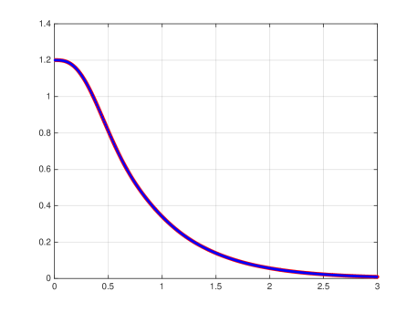
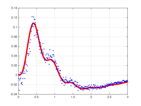
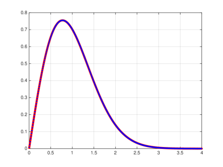
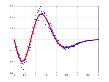
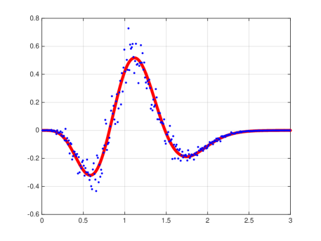
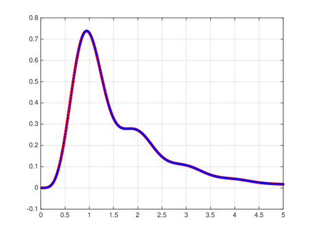
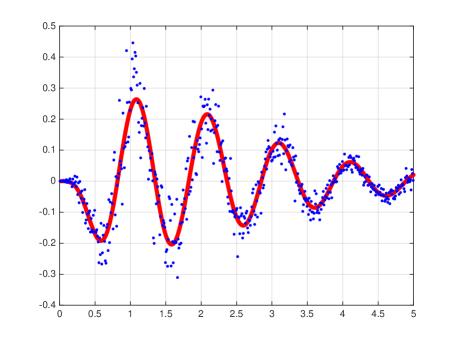
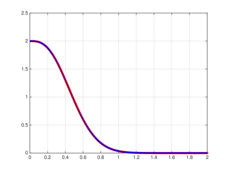
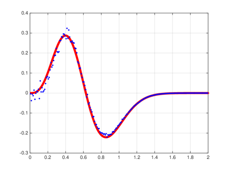
Figure 1. Minimum spacing from a randomly chosen origin: simulation vs. theory for finite size CUE, no thinning (ξ=1𝜉1\xi=1). Left panel: a histogram of empirical data from CUENsubscriptCUE𝑁{\rm CUE}_{N} with N=20𝑁20N=20 scaled to unit mean spacing, computed using a bin size of 0.01 and 108superscript10810^{8} samples from CUENsubscriptCUE𝑁{\rm CUE}_{N}, for each of which 100010001000 samples of a uniformly distributed random origin were drawn (blue dots); the large N𝑁N limit pOrigin,ξ(s)subscript𝑝Origin𝜉𝑠p_{{\rm Origin},\xi}(s) (red solid line). Right panel: the simulation data minus pOrigin,ξ(s)subscript𝑝Origin𝜉𝑠p_{{\rm Origin},\xi}(s) scaled by N2superscript𝑁2N^{2} (blue dots); the leading correction term rOrigin,ξ(s)subscript𝑟Origin𝜉𝑠r_{{\rm Origin},\xi}(s) (red solid line).
Refer to caption
Refer to caption
Figure 2. As in Figure 1 but with thinning ξ=0.6𝜉0.6\xi=0.6.

3.4. Minimum spacing distribution from a randomly chosen origin

The quantity ECβE(0;(s,s))superscript𝐸C𝛽E0𝑠𝑠E^{{\rm C}\beta{\rm E}}(0;(-s,s)) is the probability that there are no eigenvalues in the interval (s,s)𝑠𝑠(-s,s) of the scaled Cβ𝛽\betaE. Differentiating this quantity with respect to s𝑠s gives the probability density function pOriginCβE(s)superscriptsubscript𝑝OriginC𝛽E𝑠p_{\rm Origin}^{{\rm C}\beta{\rm E}}(s) for the scaled eigen-angle closest to the origin,

pOriginCβE(s)=ddsECβE(0;(s,s)).superscriptsubscript𝑝OriginC𝛽E𝑠𝑑𝑑𝑠superscript𝐸C𝛽E0𝑠𝑠p_{\rm Origin}^{{\rm C}\beta{\rm E}}(s)=-{d\over ds}E^{{\rm C}\beta{\rm E}}(0;(-s,s)).

In the case β=2𝛽2\beta=2 with thinning, it follows from (3.14), as well as the translation invariance of the sine kernel, that

pOrigin,ξCUE(s)=ddsdet(𝕀ξ𝕂2sN).superscriptsubscript𝑝Origin𝜉CUE𝑠𝑑𝑑𝑠𝕀𝜉superscriptsubscript𝕂2𝑠𝑁p_{\rm Origin,\xi}^{{\rm CUE}}(s)=-{d\over ds}\det(\operatorname{\mathbb{I}}-\xi\operatorname{\mathbb{K}}_{2s}^{N}). (3.21)

Use of (1.14) gives a characterisation of the leading two terms of the large N𝑁N expansion of this quantity.

Proposition 3.3.

We have

pOrigin,ξCUE(s)=pOrigin,ξ(s)+1N2rOrigin,ξ(s)+O(1N4)superscriptsubscript𝑝Origin𝜉CUE𝑠subscript𝑝Origin𝜉𝑠1superscript𝑁2subscript𝑟Origin𝜉𝑠O1superscript𝑁4p_{\rm Origin,\xi}^{{\rm CUE}}(s)=p_{\rm Origin,\xi}(s)+{1\over N^{2}}r_{\rm Origin,\xi}(s)+\operatorname{O}\Big{(}{1\over N^{4}}\Big{)} (3.22)

where in terms of integral operators

pOrigin,ξ(s)subscript𝑝Origin𝜉𝑠\displaystyle p_{\rm Origin,\xi}(s) =ddsdet(𝕀ξ𝕂2s)absent𝑑𝑑𝑠𝕀𝜉subscript𝕂2𝑠\displaystyle=-{d\over ds}\det(\operatorname{\mathbb{I}}-\xi\operatorname{\mathbb{K}}_{2s})
rOrigin,ξ(s)subscript𝑟Origin𝜉𝑠\displaystyle r_{\rm Origin,\xi}(s) =ξddsΩ(ξ𝕂2s):𝕃2s.:absent𝜉𝑑𝑑𝑠Ω𝜉subscript𝕂2𝑠subscript𝕃2𝑠\displaystyle=-\xi{d\over ds}\operatorname{\Omega}(\xi\operatorname{\mathbb{K}}_{2s}):\operatorname{\mathbb{L}}_{2s}. (3.23)

Alternatively, in terms of σ(0)superscript𝜎0\sigma^{(0)} and σ(1)superscript𝜎1\sigma^{(1)} defined in (1.14)

pOrigin,ξ(s)=ddsexp(02πsσ(0)(t;ξ)t𝑑t)subscript𝑝Origin𝜉𝑠𝑑𝑑𝑠superscriptsubscript02𝜋𝑠superscript𝜎0𝑡𝜉𝑡differential-d𝑡p_{\rm Origin,\xi}(s)=-{d\over ds}\exp\left(\int_{0}^{2\pi s}{\sigma^{(0)}(t;\xi)\over t}\,dt\right) (3.24)

and

rOrigin,ξ(s)=dds(02πsσ(1)(t;ξ)t𝑑t)exp(02πsσ(0)(t;ξ)t𝑑t).subscript𝑟Origin𝜉𝑠𝑑𝑑𝑠superscriptsubscript02𝜋𝑠superscript𝜎1𝑡𝜉𝑡differential-d𝑡superscriptsubscript02𝜋𝑠superscript𝜎0𝑡𝜉𝑡differential-d𝑡r_{\rm Origin,\xi}(s)=-{d\over ds}\Big{(}\int_{0}^{2\pi s}{\sigma^{(1)}(t;\xi)\over t}\,dt\Big{)}\exp\left(\int_{0}^{2\pi s}{\sigma^{(0)}(t;\xi)\over t}\,dt\right). (3.25)

To simulate this quantity in translationally invariant empirical data such as the CUECUE{\rm CUE} itself, one can actually draw the origin uniformly and independently within the interval for which the data are defined (that is, one superimposes a Poisson point process defining the origin). To prepare for corresponding computations within a large set of Riemann zeros this was done, as a proof of concept, for CUE matrices in Figs. 1 and Figs. 2.

3.5. Nearest neighbour spacing distribution

A variant of the spacing distribution between consecutive eigenvalues is the spacing distribution between nearest neighbour eigenvalues [20]. For this, at each eigenvalue one measures the smallest of the spacings to the eigenvalue immediately to the left, and the spacing immediately to the right. In a theoretical ensemble formulation, the system is to be conditioned so that there is an eigenvalue at the origin. Consider in particular the CUE with eigen-angles scaled to have unit spacing. With ρ(n),ξCUE,θ=0superscriptsubscript𝜌𝑛𝜉CUE𝜃0\rho_{(n),\xi}^{{\rm CUE},\theta=0} denoting the n𝑛n-point correlation function for the conditioned system in the presence of thinning, we have

ρ(n),ξCUE,θ=0(θ1,,θn)=ξnρ(n+1)CUE(θ1,,θn,0)=ξndet(sinπ(θjθk)Nsin(π(θjθk)/N)sinπθjNsinπθj/NsinπθkNsinπθk/N)j,k=1,,n,superscriptsubscript𝜌𝑛𝜉CUE𝜃0subscript𝜃1subscript𝜃𝑛superscript𝜉𝑛superscriptsubscript𝜌𝑛1CUEsubscript𝜃1subscript𝜃𝑛0superscript𝜉𝑛subscript𝜋subscript𝜃𝑗subscript𝜃𝑘𝑁𝜋subscript𝜃𝑗subscript𝜃𝑘𝑁𝜋subscript𝜃𝑗𝑁𝜋subscript𝜃𝑗𝑁𝜋subscript𝜃𝑘𝑁𝜋subscript𝜃𝑘𝑁formulae-sequence𝑗𝑘1𝑛\rho_{(n),\xi}^{{\rm CUE},\theta=0}(\theta_{1},\dots,\theta_{n})=\xi^{n}\rho_{(n+1)}^{{\rm CUE}}(\theta_{1},\dots,\theta_{n},0)\\ =\xi^{n}\det\left({\sin\pi(\theta_{j}-\theta_{k})\over N\sin(\pi(\theta_{j}-\theta_{k})/N)}-{\sin\pi\theta_{j}\over N\sin\pi\theta_{j}/N}{\sin\pi\theta_{k}\over N\sin\pi\theta_{k}/N}\right)_{j,k=1,\dots,n}, (3.26)

where the second line follows from (3.6) and (1.8), together with elementary row operations applied to the determinant.

Let the entry of the determinant in (3.26) be denoted by K~N(θj,θk)superscript~𝐾𝑁subscript𝜃𝑗subscript𝜃𝑘\tilde{K}^{N}(\theta_{j},\theta_{k}), and denote the corresponding integral operator supported on (s,s)𝑠𝑠(-s,s) by 𝕂~(s,s)Nsubscriptsuperscript~𝕂𝑁𝑠𝑠\tilde{\operatorname{\mathbb{K}}}^{N}_{(-s,s)}. Analogous to (3.21), the scaled nearest neighbour spacing in the presence of thinning is then

pnn,ξCUE(s)=ddsdet(𝕀ξ𝕂~(s,s)N).superscriptsubscript𝑝nn𝜉CUE𝑠𝑑𝑑𝑠𝕀𝜉superscriptsubscript~𝕂𝑠𝑠𝑁p_{\rm nn,\xi}^{{\rm CUE}}(s)=-{d\over ds}\det\Big{(}\operatorname{\mathbb{I}}-\xi\tilde{\operatorname{\mathbb{K}}}_{(-s,s)}^{N}\Big{)}. (3.27)

By observing

K~N(x,y)=KN(x,y)KN(x,0)KN(0,y)superscript~𝐾𝑁𝑥𝑦superscript𝐾𝑁𝑥𝑦superscript𝐾𝑁𝑥0superscript𝐾𝑁0𝑦\tilde{K}^{N}(x,y)=K^{N}(x,y)-K^{N}(x,0)K^{N}(0,y)

we can read off from (3.27), upon expanding the kernel to order 1/N21superscript𝑁21/N^{2}, integral operator formulae for the leading two terms analogous to (3.3).

Proposition 3.4.
In terms of the notation (1.3) and (1.10), let

Knn(x,y)superscript𝐾nn𝑥𝑦\displaystyle{K}^{\rm nn}(x,y) =K(x,y)K(x,0)K(0,y)absent𝐾𝑥𝑦𝐾𝑥0𝐾0𝑦\displaystyle=K(x,y)-K(x,0)K(0,y)
Lnn(x,y)superscript𝐿nn𝑥𝑦\displaystyle{L}^{\rm nn}(x,y) =L(x,y)L(x,0)K(0,y)K(x,0)L(0,y).absent𝐿𝑥𝑦𝐿𝑥0𝐾0𝑦𝐾𝑥0𝐿0𝑦\displaystyle=L(x,y)-L(x,0)K(0,y)-K(x,0)L(0,y). (3.28)

Denote by 𝕂(s,s)nnsuperscriptsubscript𝕂𝑠𝑠nn{\operatorname{\mathbb{K}}}_{(-s,s)}^{\rm nn} and 𝕃(s,s)nnsuperscriptsubscript𝕃𝑠𝑠nn{\operatorname{\mathbb{L}}}_{(-s,s)}^{\rm nn} the integral operators on (s,s)𝑠𝑠(-s,s) with kernels Knn(x,y)superscript𝐾nn𝑥𝑦{K}^{\rm nn}(x,y) and Lnn(x,y)superscript𝐿nn𝑥𝑦{L}^{\rm nn}(x,y) respectively. We have

pnn,ξCUE(s)=pnn,ξ(s)+1N2rnn,ξ(s)+O(1N4),superscriptsubscript𝑝nn𝜉CUE𝑠subscript𝑝nn𝜉𝑠1superscript𝑁2subscript𝑟nn𝜉𝑠O1superscript𝑁4p_{\rm nn,\xi}^{{\rm CUE}}(s)=p_{\rm nn,\xi}(s)+{1\over N^{2}}r_{\rm nn,\xi}(s)+\operatorname{O}\Big{(}{1\over N^{4}}\Big{)}, (3.29)

where

pnn,ξ(s)subscript𝑝nn𝜉𝑠\displaystyle p_{\rm nn,\xi}(s) =ddsdet(𝕀ξ𝕂(s,s)nn)absent𝑑𝑑𝑠𝕀𝜉superscriptsubscript𝕂𝑠𝑠nn\displaystyle=-{d\over ds}\det\left(\operatorname{\mathbb{I}}-\xi{\operatorname{\mathbb{K}}}_{(-s,s)}^{\rm nn}\right)
rnn,ξ(s)subscript𝑟nn𝜉𝑠\displaystyle r_{\rm nn,\xi}(s) =ξddsΩ(ξ𝕂(s,s)nn):𝕃(s,s)nn.:absent𝜉𝑑𝑑𝑠Ω𝜉superscriptsubscript𝕂𝑠𝑠nnsuperscriptsubscript𝕃𝑠𝑠nn\displaystyle=-\xi{d\over ds}\operatorname{\Omega}(\xi{\operatorname{\mathbb{K}}}_{(-s,s)}^{\rm nn}):{\operatorname{\mathbb{L}}}_{(-s,s)}^{\rm nn}. (3.30)
Remark 3.5.

In [20] a Painlevé transcendent evaluation of pnn,ξ(s)subscript𝑝nn𝜉𝑠p_{\rm nn,\xi}(s) has been given; see also [18, §9.5.2].

Refer to caption
Refer to caption
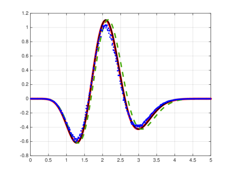
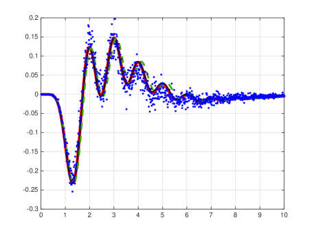
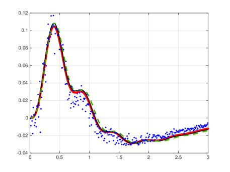
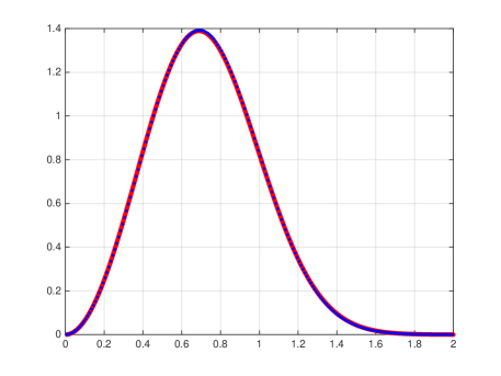
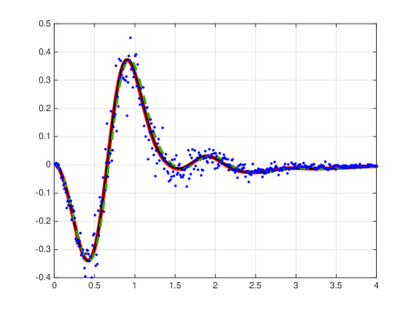
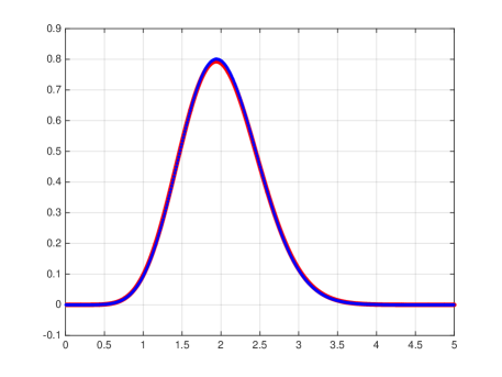
Figure 3. 111-st next neighbour spacing: Riemann zeros data vs. random-matrix based prediction with effective dimension N=log(E/2π)/12Λ11.3𝑁𝐸2𝜋12Λ11.3N=\log(E/2\pi)/\sqrt{12\Lambda}\approx 11.3, no thinning (ξ=1𝜉1\xi=1). Left panel: a histogram of the Odlyzko data set with bin size 0.010.010.01 (blue dots); the large N𝑁N limit p2,ξ(1;s)subscript𝑝2𝜉1𝑠p_{2,\xi}(1;s) (red solid line). Right panel: the Riemann zero data minus p2,ξ(1;s)subscript𝑝2𝜉1𝑠p_{2,\xi}(1;s) scaled by N2superscript𝑁2N^{2} (blue dots); the leading correction term r2,ξ(1;s)subscript𝑟2𝜉1𝑠r_{2,\xi}(1;s) with interior rescaling (red solid line), exterior rescaling (thin black line) and no rescaling (dashed green line).

4. Application to the statistics of Riemann zeros

4.1. The two point correlation function

Starting with the 1973 seminal work of Montgomery there have been significant developments on a deep (conjectural) connection between the statistics of the fluctuation properties of the zeros of the Riemann zeta function on the critical axis Res=1/2Re𝑠12\operatorname{\rm Re}s=1/2 and those of the eigen-angles of CUENsubscriptCUE𝑁{\rm CUE}_{N}, supported by large-scale numerical calculations based on the extensive tables of Riemann zeros provides by Odlyzko, see, e.g., [35, 20, 3, 29, 36, 5, 19] and the literature cited therein. Answering a question of Odlyzko [36], who had posed the challenge of understanding the structure in the numerical difference graph between the Riemann zeta spacing distribution for a set of zeros of large height and the (conjectured) asymptotics, finite size effects of this statistic were studied in [5]. This study gave a precise quantitative association of Riemann zeros 1/2+iE12𝑖𝐸1/2+iE at height E𝐸E to a (formal) size N𝑁N of the corresponding CUENsubscriptCUE𝑁{\rm CUE}_{N}. Using the Hardy–Littlewood conjecture of the distribution of prime pairs, Bogomonly and Keating [6] had earlier given an analytic expression for the pair correlation of the Riemann zeros. The authors of [5] expanded this for large height E𝐸E, with the local density normalized to unity, to obtain

R2RZ(s)=1sin2(πs)π2s2Λsin2(πs)π2ρ¯2Qssin(2πs)2π2ρ¯3+O(ρ¯4),subscriptsuperscript𝑅RZ2𝑠1superscript2𝜋𝑠superscript𝜋2superscript𝑠2Λsuperscript2𝜋𝑠superscript𝜋2superscript¯𝜌2𝑄𝑠2𝜋𝑠2superscript𝜋2superscript¯𝜌3Osuperscript¯𝜌4R^{\text{RZ}}_{2}(s)=1-\frac{\sin^{2}(\pi s)}{\pi^{2}s^{2}}-\frac{\Lambda\sin^{2}(\pi s)}{\pi^{2}}\bar{\rho}^{-2}-\frac{Qs\sin(2\pi s)}{2\pi^{2}}\bar{\rho}^{-3}+\operatorname{O}(\bar{\rho}^{-4}), (4.1)

where

ρ¯=log(E/2π)2π¯𝜌𝐸2𝜋2𝜋\bar{\rho}=\frac{\log(E/2\pi)}{2\pi}

denotes the smooth asymptotic density of zeros at E𝐸E and ΛΛ\Lambda, Q𝑄Q are the following constants (with γnsubscript𝛾𝑛\gamma_{n} the Stieltjes constants and psubscript𝑝\sum_{p} summation over the primes):444The highly accurate numerical values were obtained by applying the Euler–Maclaurin formula to the Stieltjes constants, γn=limm(k=1mlognkklogn+1mm+1),subscript𝛾𝑛subscript𝑚superscriptsubscript𝑘1𝑚superscript𝑛𝑘𝑘superscript𝑛1𝑚𝑚1\gamma_{n}=\lim_{m\to\infty}\left(\sum_{k=1}^{m}\frac{\log^{n}k}{k}-\frac{\log^{n+1}m}{m+1}\right), and the method of [31, p. 2] to the sums over the primes.

ΛΛ\displaystyle\Lambda =γ02+2γ1+plog2p(p1)2=1.57315 10713 24955,absentsuperscriptsubscript𝛾022subscript𝛾1subscript𝑝superscript2𝑝superscript𝑝121.573151071324955\displaystyle=\gamma_{0}^{2}+2\gamma_{1}+\sum_{p}\frac{\log^{2}p}{(p-1)^{2}}=1.57315\,10713\,24955\,\ldots,
Q𝑄\displaystyle Q =plog3p(p1)2=2.31584 63849 58803.absentsubscript𝑝superscript3𝑝superscript𝑝122.315846384958803\displaystyle=\sum_{p}\frac{\log^{3}p}{(p-1)^{2}}=2.31584\,63849\,58803\,\ldots.

On the other hand, the pair correlation function

R2CUEN(s)=ρ(2)(0,s)=|KN(0,0)KN(0,s)KN(s,0)KN(s,s)|subscriptsuperscript𝑅subscriptCUE𝑁2𝑠subscript𝜌20𝑠matrixsuperscript𝐾𝑁00superscript𝐾𝑁0𝑠superscript𝐾𝑁𝑠0superscript𝐾𝑁𝑠𝑠R^{\text{CUE}_{N}}_{2}(s)=\rho_{(2)}(0,s)=\begin{vmatrix}K^{N}(0,0)&K^{N}(0,s)\\ K^{N}(s,0)&K^{N}(s,s)\end{vmatrix}

of CUENsubscriptCUE𝑁{\rm CUE}_{N}, normalized to mean spacing unity, expands by (1.9) as

R2CUE(s)=ρ(2)(x,x+s)=1sin2(πs)π2s2sin2(πs)3N2+O(N4).subscriptsuperscript𝑅CUE2𝑠subscript𝜌2𝑥𝑥𝑠1superscript2𝜋𝑠superscript𝜋2superscript𝑠2superscript2𝜋𝑠3superscript𝑁2Osuperscript𝑁4R^{\text{CUE}}_{2}(s)=\rho_{(2)}(x,x+s)=1-\frac{\sin^{2}(\pi s)}{\pi^{2}s^{2}}-\frac{\sin^{2}(\pi s)}{3}N^{-2}+\operatorname{O}(N^{-4}). (4.2)

By matching the first correction terms of (4.1) and (4.2) the authors of [5] got as effective dimension N𝑁N of a CUENsubscriptCUE𝑁{\rm CUE}_{N} at height E𝐸E

N=π3Λρ¯=112Λlog(E2π).𝑁𝜋3Λ¯𝜌112Λ𝐸2𝜋N=\frac{\pi}{\sqrt{3\Lambda}}\bar{\rho}=\frac{1}{\sqrt{12\Lambda}}\log\left(\frac{E}{2\pi}\right).

This way one has the (conjectural) approximation
R2RZ(s)=R2CUE(s)+O(N3).superscriptsubscript𝑅2RZ𝑠superscriptsubscript𝑅2CUE𝑠Osuperscript𝑁3R_{2}^{\text{RZ}}(s)=R_{2}^{\text{CUE}}(s)+\operatorname{O}(N^{-3}).
Refer to caption
Refer to caption
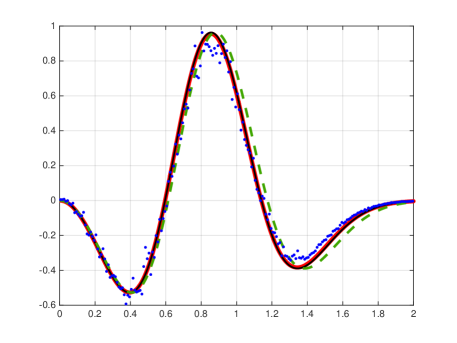
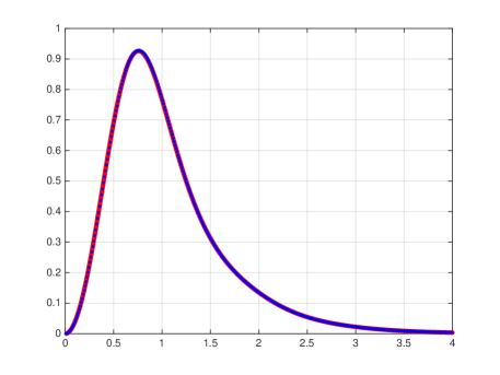
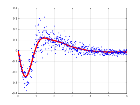
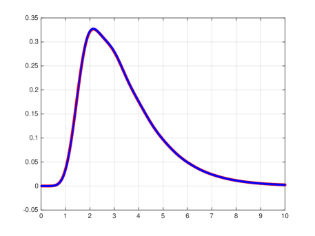
Figure 4. As in Figure 3 but with thinning ξ=0.6𝜉0.6\xi=0.6.

4.2. Exterior rescaling of the leading correction terms

As noted in [5] a rescaling of the s𝑠s-variable in the leading correction term of the ρ¯¯𝜌\bar{\rho}-expansion of the two-point functions absorbs the O(ρ¯3)Osuperscript¯𝜌3\operatorname{O}(\bar{\rho}^{-3}) term, respectively the O(N3)Osuperscript𝑁3\operatorname{O}(N^{-3}) term:

R2RZ(s)subscriptsuperscript𝑅RZ2𝑠\displaystyle R^{\text{RZ}}_{2}(s) =1sin2(πs)π2s2Λsin2(παs)π2ρ¯2+O(ρ¯4)absent1superscript2𝜋𝑠superscript𝜋2superscript𝑠2Λsuperscript2𝜋𝛼𝑠superscript𝜋2superscript¯𝜌2Osuperscript¯𝜌4\displaystyle=1-\frac{\sin^{2}(\pi s)}{\pi^{2}s^{2}}-\frac{\Lambda\sin^{2}(\pi\alpha s)}{\pi^{2}}\bar{\rho}^{-2}+\operatorname{O}(\bar{\rho}^{-4})
=1sin2(πs)π2s2sin2(παs)3N2+O(N4),absent1superscript2𝜋𝑠superscript𝜋2superscript𝑠2superscript2𝜋𝛼𝑠3superscript𝑁2Osuperscript𝑁4\displaystyle=1-\frac{\sin^{2}(\pi s)}{\pi^{2}s^{2}}-\frac{\sin^{2}(\pi\alpha s)}{3}N^{-2}+\operatorname{O}(N^{-4}),

where

α=1+Q2πΛρ¯=1+QΛlog(E/2π)=1+QΛ12ΛN1.𝛼1𝑄2𝜋Λ¯𝜌1𝑄Λ𝐸2𝜋1𝑄Λ12Λsuperscript𝑁1\alpha=1+\frac{Q}{2\pi\Lambda\bar{\rho}}=1+\frac{Q}{\Lambda\log(E/2\pi)}=1+\frac{Q}{\Lambda\sqrt{12\Lambda}}N^{-1}.

That is, one gets an O(N4)𝑂superscript𝑁4O(N^{-4}) approximation of R2RZ(s)subscriptsuperscript𝑅RZ2𝑠R^{\text{RZ}}_{2}(s) by expanding R2CUE(s)subscriptsuperscript𝑅CUE2𝑠R^{\text{CUE}}_{2}(s) into powers of N2superscript𝑁2N^{-2} and rescaling the s𝑠s-variable of the leading correction term by α𝛼\alpha.

It was suggested in [5] to apply the same procedure, that is, α𝛼\alpha-rescaling the s𝑠s-variable of the leading correction term of a CUENsubscriptCUE𝑁{\rm CUE}_{N} based expansion, to improve the fit even for more general statistics, such as the spacing distribution originally considered by Odlyzko. In [19] it was successfully applied to improve the fit of the CUE leading correction term to the spacing distribution in the presence of thinning.

Refer to caption
Refer to caption
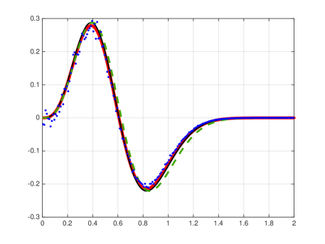
Figure 5. Minimum spacing from a randomly chosen origin: Riemann zeros data vs. random-matrix based prediction with effective dimension N=log(E/2π)/12Λ11.3𝑁𝐸2𝜋12Λ11.3N=\log(E/2\pi)/\sqrt{12\Lambda}\approx 11.3, no thinning (ξ=1𝜉1\xi=1). Left panel: a histogram of the Odlyzko data set with bin size 0.010.010.01 (blue dots), where the approximately 109superscript10910^{9} zeros were broken into 1024 sets of nearly equal size, for each of which 107superscript10710^{7} samples of a uniformly distributed random origin were drawn; the large N𝑁N limit pOrigin,ξ(s)subscript𝑝Origin𝜉𝑠p_{{\rm Origin},\xi}(s) (red solid line). Right panel: the Riemann zero data minus pOrigin,ξ(s)subscript𝑝Origin𝜉𝑠p_{{\rm Origin},\xi}(s) scaled by N2superscript𝑁2N^{2} (blue dots); the leading correction term rOrigin,ξ(s)subscript𝑟Origin𝜉𝑠r_{{\rm Origin},\xi}(s) with interior rescaling (red solid line), exterior rescaling (thin black line) and no rescaling (dashed green line).
Refer to caption
Refer to caption
Figure 6. As in Figure 5 but with thinning ξ=0.6𝜉0.6\xi=0.6.

4.3. Interior rescaling of the leading correction terms

The numerical data, physical arguments and mathematical conjectures surrounding the fluctuations of the Riemann zeros indicate that their statistics are asymptotically well approximated, to more than just leading order, by some correlation kernel KRZNsuperscriptsubscript𝐾RZ𝑁K_{\rm RZ}^{N}. Consequently, to justify the mechanism of the exterior rescaling introduced in the last paragraph, [5, p. 10748] suggested to pull-back the absorption of the O(ρ¯3)Osuperscript¯𝜌3\operatorname{O}(\bar{\rho}^{-3}) term from the two-point function into the expansion of such an assumed kernel. In the present paper we will use such an expansion to improve systematically the CUENsubscriptCUE𝑁{\rm CUE}_{N} fit of the fluctuation properties of the Riemann zeros statistics from O(N3)Osuperscript𝑁3\operatorname{O}(N^{-3}) to O(N4)Osuperscript𝑁4\operatorname{O}(N^{-4}).

By modifying the expansion (1.9) of the CUE correlation kernel KNsuperscript𝐾𝑁K^{N} to include an O(N3)Osuperscript𝑁3\operatorname{O}(N^{-3}) term,

KRZN(x,y)=K(x,y)+L(x,y)N2+M(x,y)N3+O(N4),superscriptsubscript𝐾RZ𝑁𝑥𝑦𝐾𝑥𝑦𝐿𝑥𝑦superscript𝑁2𝑀𝑥𝑦superscript𝑁3Osuperscript𝑁4K_{\rm RZ}^{N}(x,y)=K(x,y)+L(x,y)N^{-2}+M(x,y)N^{-3}+\operatorname{O}(N^{-4}), (4.3)

the task is thus to identify the unknown kernel M(x,y)𝑀𝑥𝑦M(x,y) from the O(N3)Osuperscript𝑁3\operatorname{O}(N^{-3}) term in (4.1). By translation invariance and symmetry of the kernel KRZNsuperscriptsubscript𝐾RZ𝑁K_{\rm RZ}^{N} and by the normalization KRZN(x,x)=1superscriptsubscript𝐾RZ𝑁𝑥𝑥1K_{\rm RZ}^{N}(x,x)=1 to mean spacing unity, we get the form

M(x,y)=μ(xy)𝑀𝑥𝑦𝜇𝑥𝑦M(x,y)=\mu(x-y)

of a convolution kernel with a symmetric function μ𝜇\mu satisfying μ(0)=0𝜇00\mu(0)=0. A brief calculation results in the corresponding two-point function

R2RZ(s)=1sin2(πs)π2s2sin2(πs)3N22μ(s)sin(πs)πsN3+O(N4).superscriptsubscript𝑅2RZ𝑠1superscript2𝜋𝑠superscript𝜋2superscript𝑠2superscript2𝜋𝑠3superscript𝑁22𝜇𝑠𝜋𝑠𝜋𝑠superscript𝑁3Osuperscript𝑁4R_{2}^{\rm RZ}(s)=1-\frac{\sin^{2}(\pi s)}{\pi^{2}s^{2}}-\frac{\sin^{2}(\pi s)}{3}N^{-2}-\frac{2\mu(s)\sin(\pi s)}{\pi s}N^{-3}+\operatorname{O}(N^{-4}).

Matching with (4.1) gives, cf. the first equality in [5, Eq. (28)],

μ(s)=ηπ2s2cos(πs)6,η=QΛ3Λ.formulae-sequence𝜇𝑠𝜂superscript𝜋2superscript𝑠2𝜋𝑠6𝜂𝑄Λ3Λ\mu(s)=\eta\frac{\pi^{2}s^{2}\cos(\pi s)}{6},\qquad\eta=\frac{Q}{\Lambda\sqrt{3\Lambda}}.

In the appendix of [5] it is shown that this expansion of the kernel allows one to consistently reproduce a conjectural expansion of the three-point function (which was obtained from a calculation published much later in [7]). This is further evidence that the kernel expansion (4.3) induces, quite generally, the O(N3)𝑂superscript𝑁3O(N^{-3}) correction terms in the determinantal point process fluctuation statistics.

Now, the correction kernel M𝑀M can be absorbed easily by an interior rescaling of the leading correction kernel L𝐿L, namely by introducing

LRZ(x,y)=π(xy)sin(πα¯(xy))6,subscript𝐿RZ𝑥𝑦𝜋𝑥𝑦𝜋¯𝛼𝑥𝑦6L_{\rm RZ}(x,y)=\frac{\pi(x-y)\sin(\pi\bar{\alpha}(x-y))}{6}, (4.4)

which expands as LRZ(x,y)=L(x,y)+M(x,y)N1+O(N2)subscript𝐿RZ𝑥𝑦𝐿𝑥𝑦𝑀𝑥𝑦superscript𝑁1Osuperscript𝑁2L_{\rm RZ}(x,y)=L(x,y)+M(x,y)N^{-1}+\operatorname{O}(N^{-2}), where555Note that [5, Eq. (28)] contains a miscalculation by claiming that α¯¯𝛼\bar{\alpha} would be the same as α𝛼\alpha.

α¯=1+ηN1=1+QπΛρ¯=1+2QΛlog(E/2π)=2α1.¯𝛼1𝜂superscript𝑁11𝑄𝜋Λ¯𝜌12𝑄Λ𝐸2𝜋2𝛼1\bar{\alpha}=1+\eta N^{-1}=1+\frac{Q}{\pi\Lambda\bar{\rho}}=1+\frac{2Q}{\Lambda\log(E/2\pi)}=2\alpha-1. (4.5)

To summarize, we have

KRZN(x,y)=K(x,y)+LRZ(x,y)N2+O(N4)superscriptsubscript𝐾RZ𝑁𝑥𝑦𝐾𝑥𝑦subscript𝐿RZ𝑥𝑦superscript𝑁2Osuperscript𝑁4K_{\rm RZ}^{N}(x,y)=K(x,y)+L_{\rm RZ}(x,y)N^{-2}+\operatorname{O}(N^{-4}) (4.6)

and thus get the following recipe to go from the leading correction term of a CUENsubscriptCUE𝑁{\rm CUE}_{N} fluctuation statistics to the corresponding one of the Riemann zeros: simply replace the leading correction kernel L𝐿L by its interior rescaling LRZsubscript𝐿RZL_{\rm RZ}.

In our experiments, the most pronounced difference between interior and exterior rescaling can be observed in the statistics shown in the right panel of Fig. 6.

4.4. The Odlyzko data set

The largest data set of Riemann zeros currently provided by Odlyzko, which was announced already in [36], consists of the 1 041 719 07510417190751\,041\,719\,075 consecutive zeros starting with zero number

1023+985 531 550.superscript102398553155010^{23}+985\,531\,550.

The first of them has height

13 066 434 408 793 621 120 027.39614 65854,13066434408793621120027.396146585413\,066\,434\,408\,793\,621\,120\,027.39614\,65854\ldots,

while the last one has height

13 066 434 408 793 754 462 591.63384 74590.13066434408793754462591.633847459013\,066\,434\,408\,793\,754\,462\,591.63384\,74590\ldots.

Because of the logarithmic dependence on the height, even within that large data set the smooth density ρ¯¯𝜌\bar{\rho}, the effective dimension N𝑁N and the scaling parameters α𝛼\alpha, α¯¯𝛼\bar{\alpha} remain essentially constant to 15 digits precision,

ρ¯¯𝜌\displaystyle\bar{\rho} =7.81235 22019 1727,absent7.81235220191727\displaystyle=7.81235\,22019\,1727\ldots,
N𝑁\displaystyle N =11.29759 09009 547,absent11.2975909009547\displaystyle=11.29759\,09009\,547\ldots,
α𝛼\displaystyle\alpha =1.02999 00807 6719,absent1.02999008076719\displaystyle=1.02999\,00807\,6719\ldots,
α¯¯𝛼\displaystyle\bar{\alpha} =1.05998 01615 3438.absent1.05998016153438\displaystyle=1.05998\,01615\,3438\ldots.

From this data set we extracted various spacing statistics,666The 00-th next neighbour spacing can be found in [36, Figs. 1–2] (no thinning and no theoretical prediction of the leading correction term), in [5, Figs. 1–3] (no thinning, exterior rescaling only) and in [19, Figs. 9–10] (exterior rescaling only). Since in this case there is no difference visible between interior and exterior rescaling we refrained from showing the results once more. with (ξ=0.6𝜉0.6\xi=0.6) and without (ξ=1𝜉1\xi=1) thinning, and compared them up to the leading correction with the theoretical prediction in terms of operator determinants det(𝕀𝕂)𝕀𝕂\det(\operatorname{\mathbb{I}}-\operatorname{\mathbb{K}}) and their corrections Ω(𝕂):𝕃:Ω𝕂𝕃\operatorname{\Omega}(\operatorname{\mathbb{K}}):\operatorname{\mathbb{L}} as obtained in Section 3 for the CUE. In Figs. 38 the Riemann zero data are shown as blue dots, the leading order term as a red solid line, and the correction terms

  • with interior rescaling LLRZ𝐿subscript𝐿RZL\to L_{\rm RZ} as a red solid line,

  • with exterior rescaling sαs𝑠𝛼𝑠s\to\alpha s as a thin black line,

  • without rescaling as a green dashed line.

In particular, the following statistics of the Riemann zeros are shown to be in excellent agreement up to the leading correction term with (interior) rescaling:

spacing density CUE case no thinning thinning ξ=0.6𝜉0.6\xi=0.6
111-st next neighbour pξRZ(1;s)subscriptsuperscript𝑝RZ𝜉1𝑠p^{\rm RZ}_{\xi}(1;s) Section 3.3 Fig. 3 Fig. 4
random origin pOrigin,ξRZ(s)subscriptsuperscript𝑝RZOrigin𝜉𝑠p^{\rm RZ}_{{\rm Origin},\xi}(s) Section 3.4 Fig. 5 Fig. 6
nearest neighbour pnn,ξRZ(s)subscriptsuperscript𝑝RZnn𝜉𝑠p^{\rm RZ}_{{\rm nn},\xi}(s) Section 3.5 Fig. 7 Fig. 8

Here we denote by pRZsubscriptsuperscript𝑝RZp^{\rm RZ}_{\;\ldots} those probability densities for the Riemann zeros that are defined analogously to the CUE case pCUEsubscriptsuperscript𝑝CUEp^{\rm CUE}_{\;\;\ldots}.

Refer to caption
Refer to caption
Figure 7. Nearest neighbour spacing: Riemann zeros data vs. random-matrix based prediction with effective dimension N=log(E/2π)/12Λ11.3𝑁𝐸2𝜋12Λ11.3N=\log(E/2\pi)/\sqrt{12\Lambda}\approx 11.3, no thinning (ξ=1𝜉1\xi=1). Left panel: a histogram of the Odlyzko data set with bin size 0.010.010.01 (blue dots); the large N𝑁N limit pnn,ξ(s)subscript𝑝nn𝜉𝑠p_{{\rm nn},\xi}(s) (red solid line). Right panel: the Riemann zero data minus pnn,ξ(s)subscript𝑝nn𝜉𝑠p_{{\rm nn},\xi}(s) scaled by N2superscript𝑁2N^{2} (blue dots); the leading correction term rnn,ξ(s)subscript𝑟nn𝜉𝑠r_{{\rm nn},\xi}(s) with interior rescaling (red solid line), exterior rescaling (thin black line) and no rescaling (dashed green line).
Refer to caption
Refer to caption
Figure 8. As in Figure 7 but with thinning ξ=0.6𝜉0.6\xi=0.6.

5. Spacing distributions for the COE and CSE

5.1. Generating functions

As already mentioned, the fact that the eigenvalues of COE matrices form a Pfaffian point process tells us that the counterpart to the formula (3.6) involves a Pfaffian of a 2×2222\times 2 anti-symmetric kernel function. Substituting this in (3.5), the Pfaffian analogue of the identity implying (3.7) (see e.g. [18, Eq. (6.32)]) allows for a Pfaffian analogue in the case of the COE to be given. However, the resulting formula is not of the same practical utility as (3.7) since the 2×2222\times 2 kernel function is not analytic, which in turn means that the numerical quadrature methods of Section 2.2 have poor convergence properties.

Fortunately, there is a second option. This presents itself due to fundamental inter-relations between gap probabilities for the COE and CUE. These also involve the gap probabilities for Haar distributed orthogonal matrices from the classical groups O(N)+{}^{+}(N) and O(N){}^{-}(N). In reference to the latter, eigenvalues on the real axis and thus corresponding to θ=0𝜃0\theta=0 or π𝜋\pi are to be disregarded, and only the eigenvalues with angles in (0,π)0𝜋(0,\pi) are to be considered (the remaining eigenvalues occur at the negative of these angles, i.e. the complex conjugates). The first inter-relation of interest is between the generating functions for the gap probabilities in the CUE, and in Haar distributed real orthogonal matrices [2, 17], [18, Eq. (8.127)]

CUE((θ,θ);z)=O(2(N+1)/2+1)((0,θ);z)O+(2N/2+1)((0,θ);z).superscriptCUE𝜃𝜃𝑧superscriptsuperscriptO2𝑁1210𝜃𝑧superscriptsuperscriptO2𝑁210𝜃𝑧{\mathcal{E}}^{\rm CUE}((-\theta,\theta);z)={\mathcal{E}}^{\operatorname{O}^{-}(2\lfloor(N+1)/2\rfloor+1)}((0,\theta);z){\mathcal{E}}^{\operatorname{O}^{+}(2\lfloor N/2\rfloor+1)}((0,\theta);z). (5.1)

With ME denoting a particular matrix ensemble, we have used the symbol MEsuperscriptME{\mathcal{E}}^{\rm ME} instead of EMEsuperscript𝐸MEE^{\rm ME} to indicate that in this expression no scaling of the eigen-angles has been imposed; this convention will be followed below. In fact we only use the scaled quantity for ensembles ME=CβENMEC𝛽subscriptE𝑁{\rm ME}={\rm C}\beta{\rm E}_{N} which are translationally invariant with uniform density N/2π𝑁2𝜋N/2\pi. The unscaled and scaled quantities are then related by

CβEN((2πs/N,2πs/N);z)=ECβEN(2s;z).superscriptC𝛽subscriptE𝑁2𝜋𝑠𝑁2𝜋𝑠𝑁𝑧superscript𝐸C𝛽subscriptE𝑁2𝑠𝑧{\mathcal{E}}^{{\rm C}\beta{\rm E}_{N}}((-2\pi s/N,2\pi s/N);z)=E^{{\rm C}\beta{\rm E}_{N}}(2s;z).

To present the next inter-relation, introduce the generating functions

ECOE,±((θ,θ);z):=n=0N(1z)n(ECOE(2n,(0,θ))+ECOE(2n±1,(0,θ))).assignsuperscript𝐸COEplus-or-minus𝜃𝜃𝑧superscriptsubscript𝑛0𝑁superscript1𝑧𝑛superscript𝐸COE2𝑛0𝜃superscript𝐸COEplus-or-minus2𝑛10𝜃E^{{\rm COE},\pm}((-\theta,\theta);z):=\sum_{n=0}^{N}(1-z)^{n}\Big{(}E^{{\rm COE}}(2n,(0,\theta))+E^{{\rm COE}}(2n\pm 1,(0,\theta))\Big{)}. (5.2)

With COE\,\cup\,COE denoting the point process of 2N2𝑁2N eigenvalues on the circle that results by superimposing the eigenvalue sequences of two independent COE matrices, a result conjectured by Dyson [14] and proved by Gunson [24] gives that

alt(COECOE)=CUE,altCOECOECUE{\rm alt}\left({\rm COE}\,\cup\,{\rm COE}\right)={\rm CUE}, (5.3)

where the operation “alt" refers to the operation of observing every second eigenvalue only. As a consequence of this, one has that [14], [33]

ECUE((θ,θ);z)=ECOE,((θ,θ);z)ECOE,+((θ,θ);z).superscript𝐸CUE𝜃𝜃𝑧superscript𝐸COE𝜃𝜃𝑧superscript𝐸COE𝜃𝜃𝑧E^{\rm CUE}((-\theta,\theta);z)=E^{{\rm COE},-}((-\theta,\theta);z)E^{{\rm COE},+}((-\theta,\theta);z). (5.4)

According to (5.1), it follows from (5.4) that the gap probabilities for the COE are related to those for O(n)+{}^{+}(n) and O(n){}^{-}(n) with n𝑛n suitably chosen, but this alone does not determine the former. To be able to do this, additional inter-relationships between generating functions are required. In the case N2Nmaps-to𝑁2𝑁N\mapsto 2N and thus N𝑁N even, the additional inter-relationships have been given in [17] according to the generating function identity

COE,±((θ,θ);z)|N2N=O±(2N+1)((0,θ);z).evaluated-atsuperscriptCOEplus-or-minus𝜃𝜃𝑧maps-to𝑁2𝑁superscriptsuperscriptOplus-or-minus2𝑁10𝜃𝑧{\mathcal{E}}^{{\rm COE},\pm}((-\theta,\theta);z)\Big{|}_{N\mapsto 2N}={\mathcal{E}}^{\operatorname{O}^{\pm}(2N+1)}((0,\theta);z). (5.5)

Note that (5.5) substituted in (5.4) is consistent with (5.1) in the case N𝑁N even. The identity (5.5) has very recently [12] been shown to be a corollary of the identities between eigenvalue distributions

even|COE2N|=O+(2N+1),odd|COE2N|=O(2N+1).formulae-sequenceevensubscriptCOE2𝑁superscriptO2𝑁1oddsubscriptCOE2𝑁superscriptO2𝑁1{\rm even}\,|{\rm COE}_{2N}|=\operatorname{O}^{+}(2N+1),\qquad{\rm odd}\,|{\rm COE}_{2N}|=\operatorname{O}^{-}(2N+1). (5.6)

Here the notation COE2NsubscriptCOE2𝑁{\rm COE}_{2N} refers to the eigenvalue distribution of 2N×2N2𝑁2𝑁2N\times 2N COE matrices, while |COE2N|subscriptCOE2𝑁|{\rm COE}_{2N}| refers to the distribution in the circumstance that the eigenvalues with angles π<θ<0𝜋𝜃0-\pi<\theta<0 are reflected in the real axis by θθmaps-to𝜃𝜃\theta\mapsto-\theta, and thus all eigenvalues have angles between 0 and π𝜋\pi. The operation even (odd) refers to observing only those eigenvalues that occur an even (odd) number of places from θ=0𝜃0\theta=0, reading anti-clockwise.

Substituting (5.5) in (5.2), and setting z¯=2zz2¯𝑧2𝑧superscript𝑧2\bar{z}=2z-z^{2} so that 1z¯=(1z)21¯𝑧superscript1𝑧21-\bar{z}=(1-z)^{2} we obtain, after some minor manipulation, a known closed formula for the gap probabilities of COE2NsubscriptCOE2𝑁{\rm COE}_{2N} in terms of the gap probabilities for O±(2N+1)superscriptOplus-or-minus2𝑁1\operatorname{O}^{\pm}(2N+1) [18, Eq. (8.150)]

COE2N((θ,θ);z)=(1z)O+(2N+1)((0,θ);z¯)+O(2N+1)((0,θ);z¯)2z.superscriptsubscriptCOE2𝑁𝜃𝜃𝑧1𝑧superscriptsuperscriptO2𝑁10𝜃¯𝑧superscriptsuperscriptO2𝑁10𝜃¯𝑧2𝑧{\mathcal{E}}^{{\rm COE}_{2N}}((-\theta,\theta);z)={(1-z)\mathcal{E}^{\operatorname{O}^{+}(2N+1)}((0,\theta);\bar{z})+\mathcal{E}^{\operatorname{O}^{-}(2N+1)}((0,\theta);\bar{z})\over 2-z}. (5.7)

The analogue of (5.6) for COE2N1subscriptCOE2𝑁1{\rm COE}_{2N-1} allows us to deduce the analogue of (5.7). The required formulas were not known until [12] and consequently this is a new result.

Proposition 5.1.

We have

COE2N1((θ,θ);z)=(1z)O(2N)((0,θ);z¯)+O+(2N)((0,θ);z¯)2z.superscriptsubscriptCOE2𝑁1𝜃𝜃𝑧1𝑧superscriptsuperscriptO2𝑁0𝜃¯𝑧superscriptsuperscriptO2𝑁0𝜃¯𝑧2𝑧\mathcal{E}^{{\rm COE}_{2N-1}}((-\theta,\theta);z)={(1-z)\mathcal{E}^{\operatorname{O}^{-}(2N)}((0,\theta);\bar{z})+\mathcal{E}^{\operatorname{O}^{+}(2N)}((0,\theta);\bar{z})\over 2-z}. (5.8)
Proof.

We read off from [12, Th. 7.1] that

even|COE2N1|=O(2N),odd|COE2N1|=O+(2N).formulae-sequenceevensubscriptCOE2𝑁1superscriptO2𝑁oddsubscriptCOE2𝑁1superscriptO2𝑁{\rm even}\,|{\rm COE}_{2N-1}|=\operatorname{O}^{-}(2N),\qquad{\rm odd}\,|{\rm COE}_{2N-1}|=\operatorname{O}^{+}(2N). (5.9)

Substituting in (5.2) and manipulating as in the derivation of (5.7) gives (5.8). ∎

With ν=()N𝜈superscript𝑁\nu=(-)^{N} the cases (5.7) and (5.8) can be combined into a single formula that holds for both parities of N𝑁N:

COEN((θ,θ);z)=(1z)Oν(N+1)((0,θ);z¯)+Oν(N+1)((0,θ);z¯)2z.superscriptsubscriptCOE𝑁𝜃𝜃𝑧1𝑧superscriptsuperscriptO𝜈𝑁10𝜃¯𝑧superscriptsuperscriptO𝜈𝑁10𝜃¯𝑧2𝑧\mathcal{E}^{{\rm COE}_{N}}((-\theta,\theta);z)={(1-z)\mathcal{E}^{\operatorname{O}^{\nu}(N+1)}((0,\theta);\bar{z})+\mathcal{E}^{\operatorname{O}^{-\nu}(N+1)}((0,\theta);\bar{z})\over 2-z}. (5.10)

The eigenvalues for O±(N+1)superscriptOplus-or-minus𝑁1\operatorname{O}^{\pm}(N+1) in (0,π)0𝜋(0,\pi) form a determinantal point process with kernel (see e.g. [18, Prop. 5.5.3])

12π(sinN(xy)/2sin(xy)/2νsinN(x+y)/2sin(x+y)/2)=N2πKN,ν(xN/2π,yN/2π),12𝜋minus-or-plus𝑁𝑥𝑦2𝑥𝑦2𝜈𝑁𝑥𝑦2𝑥𝑦2𝑁2𝜋superscript𝐾𝑁minus-or-plus𝜈𝑥𝑁2𝜋𝑦𝑁2𝜋{1\over 2\pi}\bigg{(}{\sin N(x-y)/2\over\sin(x-y)/2}\mp\nu{\sin N(x+y)/2\over\sin(x+y)/2}\bigg{)}=\frac{N}{2\pi}K^{N,\mp\nu}(xN/2\pi,yN/2\pi), (5.11)

where

KN,±(x,y)=KN(x,y)±KN(x,y).superscript𝐾𝑁plus-or-minus𝑥𝑦plus-or-minussuperscript𝐾𝑁𝑥𝑦superscript𝐾𝑁𝑥𝑦K^{N,\pm}(x,y)=K^{N}(x,y)\pm K^{N}(x,-y). (5.12)

Scaling the eigen-angles of COENsubscriptCOE𝑁{\rm COE}_{N} to have unit mean spacing by θ=2πs/N𝜃2𝜋𝑠𝑁\theta=2\pi s/N thus yields the following result:

Corollary 5.2.

Let 𝕂sN,±subscriptsuperscript𝕂𝑁plus-or-minus𝑠\operatorname{\mathbb{K}}^{N,\pm}_{s} denote the integral operator on (0,s)0𝑠(0,s) with kernel (5.12) and denote z¯=2zz2¯𝑧2𝑧superscript𝑧2\bar{z}=2z-z^{2}. We have

ECOEN((s,s);z)=(1z)det(Iz¯𝕂sN,)+det(Iz¯𝕂sN,+)2z.superscript𝐸subscriptCOE𝑁𝑠𝑠𝑧1𝑧𝐼¯𝑧subscriptsuperscript𝕂𝑁𝑠𝐼¯𝑧subscriptsuperscript𝕂𝑁𝑠2𝑧E^{{\rm COE}_{N}}((-s,s);z)=\frac{(1-z)\det(I-\bar{z}\operatorname{\mathbb{K}}^{N,-}_{s})+\det(I-\bar{z}\operatorname{\mathbb{K}}^{N,+}_{s})}{2-z}. (5.13)

As in (3.13) thinning is expressed by EξCOEN((s,s);z)=ECOEN((s,s);ξz).superscriptsubscript𝐸𝜉subscriptCOE𝑁𝑠𝑠𝑧superscript𝐸subscriptCOE𝑁𝑠𝑠𝜉𝑧E_{\xi}^{{\rm COE}_{N}}((-s,s);z)=E^{{\rm COE}_{N}}((-s,s);\xi z).

We will now turn our attention to spacing probabilities for the CSE. These follow from knowledge of the spacing distributions for the COE. Thus one has the inter-relation [34]

altCOE2N=CSEN,altsubscriptCOE2𝑁subscriptCSE𝑁{\rm alt}\,{\rm COE}_{2N}={\rm CSE}_{N}, (5.14)

and it follows from this that

CSEN(n;(θ,θ))=COE2N(2n;(θ,θ))+12(COE2N(2n1;(θ,θ))+COE2N(2n+1;(θ,θ))).superscriptsubscriptCSE𝑁𝑛𝜃𝜃superscriptsubscriptCOE2𝑁2𝑛𝜃𝜃12superscriptsubscriptCOE2𝑁2𝑛1𝜃𝜃superscriptsubscriptCOE2𝑁2𝑛1𝜃𝜃\mathcal{E}^{{\rm CSE}_{N}}(n;(-\theta,\theta))\\ =\mathcal{E}^{{\rm COE}_{2N}}(2n;(-\theta,\theta))+{1\over 2}\Big{(}\mathcal{E}^{{\rm COE}_{2N}}(2n-1;(-\theta,\theta))+\mathcal{E}^{{\rm COE}_{2N}}(2n+1;(-\theta,\theta))\Big{)}. (5.15)

As noted in [18, Eq. (8.158)], recalling the definition (5.2), and making use too of (5.5), this gives

CSEN((θ,θ);z)=12(O+(2N+1)((0,θ);z)+O(2N+1)((0,θ);z)).superscriptsubscriptCSE𝑁𝜃𝜃𝑧12superscriptsuperscriptO2𝑁10𝜃𝑧superscriptsuperscriptO2𝑁10𝜃𝑧\mathcal{E}^{{\rm CSE}_{N}}((-\theta,\theta);z)={1\over 2}\Big{(}\mathcal{E}^{\operatorname{O}^{+}(2N+1)}((0,\theta);z)+\mathcal{E}^{\operatorname{O}^{-}(2N+1)}((0,\theta);z)\Big{)}. (5.16)

As discussed before (5.11), the kernel of the determinantal point process formed by the eigenvalues of O±(2N+1)superscriptOplus-or-minus2𝑁1\operatorname{O}^{\pm}(2N+1) is given by

NπK2N,(xN/π,yN/π).𝑁𝜋superscript𝐾2𝑁minus-or-plus𝑥𝑁𝜋𝑦𝑁𝜋\frac{N}{\pi}K^{2N,\mp}(xN/\pi,yN/\pi).

Scaling the eigen-angles of CSENsubscriptCSE𝑁{\rm CSE}_{N} to have unit mean spacing by θ=2πs/N𝜃2𝜋𝑠𝑁\theta=2\pi s/N thus yields the following result, where we use (3.13) to express the presence of thinning:

Proposition 5.3.

Let 𝕂sN,±subscriptsuperscript𝕂𝑁plus-or-minus𝑠\operatorname{\mathbb{K}}^{N,\pm}_{s} denote the integral operator on (0,s)0𝑠(0,s) with kernel (5.12). We have

EξCSEN((s,s);z)=12(det(Iξz𝕂2s2N,)+det(Iξz𝕂2s2N,+)).superscriptsubscript𝐸𝜉subscriptCSE𝑁𝑠𝑠𝑧12𝐼𝜉𝑧subscriptsuperscript𝕂2𝑁2𝑠𝐼𝜉𝑧subscriptsuperscript𝕂2𝑁2𝑠E_{\xi}^{{\rm CSE}_{N}}((-s,s);z)=\frac{1}{2}\left(\det(I-\xi z\operatorname{\mathbb{K}}^{2N,-}_{2s})+\det(I-\xi z\operatorname{\mathbb{K}}^{2N,+}_{2s})\right). (5.17)
Refer to caption
Refer to caption
Figure 9. 00-th next neighbour spacing: simulation vs. formulae from theory for finite size COE, no thinning (ξ=1𝜉1\xi=1). Left panel: a histogram of empirical data from COENsubscriptCOE𝑁{\rm COE}_{N} with N=20𝑁20N=20 scaled to unit mean spacing, computed using a bin size of 0.01 and 108superscript10810^{8} samples (blue dots); the large N𝑁N limit p1,ξ(0;s)subscript𝑝1𝜉0𝑠p_{1,\xi}(0;s) (red solid line). Right panel: the simulation data minus p1,ξ(0;s)subscript𝑝1𝜉0𝑠p_{1,\xi}(0;s) scaled by N2superscript𝑁2N^{2} (blue dots); the leading correction term r1,ξ(0,s)subscript𝑟1𝜉0𝑠r_{1,\xi}(0,s) (red solid line).
Refer to caption
Refer to caption
Figure 10. As in Figure 9 but with thinning ξ=0.6𝜉0.6\xi=0.6.

5.2. Expansion of spacing distributions

Making use of the second equation in (3.15) we get the spacing distribution

pξCOE(0;s)=1ξd2ds2EξCOEN(0;(s/2,s/2)),superscriptsubscript𝑝𝜉COE0𝑠1𝜉superscript𝑑2𝑑superscript𝑠2superscriptsubscript𝐸𝜉subscriptCOE𝑁0𝑠2𝑠2p_{\xi}^{{\rm COE}}(0;s)={1\over\xi}{d^{2}\over ds^{2}}E_{\xi}^{{\rm COE}_{N}}(0;(-s/2,s/2)), (5.18)

from which knowledge of the large N𝑁N expansion of the determinants in Corollary 5.2 will allow us to determine the terms in the corresponding expansion of the spacing.

Proposition 5.4.

Let 𝕂s±superscriptsubscript𝕂𝑠plus-or-minus\operatorname{\mathbb{K}}_{s}^{\pm} and 𝕃s±superscriptsubscript𝕃𝑠plus-or-minus\operatorname{\mathbb{L}}_{s}^{\pm} denote the integral operators on (0,s)0𝑠(0,s) with kernels K(x,y)±K(x,y)plus-or-minus𝐾𝑥𝑦𝐾𝑥𝑦K(x,y)\pm K(x,-y) and L(x,y)±L(x,y)plus-or-minus𝐿𝑥𝑦𝐿𝑥𝑦L(x,y)\pm L(x,-y) respectively. We have

pξCOE(0;s)=p1,ξ(0;s)+1N2r1,ξ(0;s)+O(1N4),subscriptsuperscript𝑝COE𝜉0𝑠subscript𝑝1𝜉0𝑠1superscript𝑁2subscript𝑟1𝜉0𝑠O1superscript𝑁4p^{{\rm COE}}_{\xi}(0;s)=p_{1,\xi}(0;s)+{1\over N^{2}}r_{1,\xi}(0;s)+\operatorname{O}\Big{(}{1\over N^{4}}\Big{)}, (5.19)

where, denoting ξ¯=2ξξ2¯𝜉2𝜉superscript𝜉2\bar{\xi}=2\xi-\xi^{2},

p1,ξ(0;s)=1ξ¯d2ds2((1ξ)det(𝕀ξ¯𝕂s/2)+det(𝕀ξ¯𝕂s/2+))subscript𝑝1𝜉0𝑠1¯𝜉superscript𝑑2𝑑superscript𝑠21𝜉𝕀¯𝜉superscriptsubscript𝕂𝑠2𝕀¯𝜉superscriptsubscript𝕂𝑠2p_{1,\xi}(0;s)={1\over\bar{\xi}}{d^{2}\over ds^{2}}\left((1-\xi)\det(\operatorname{\mathbb{I}}-\bar{\xi}\operatorname{\mathbb{K}}_{s/2}^{-})+\det(\operatorname{\mathbb{I}}-\bar{\xi}\operatorname{\mathbb{K}}_{s/2}^{+})\right) (5.20)

and

r1,ξ(0;s)=d2ds2((1ξ)Ω(ξ¯𝕂s/2):𝕃s/2+Ω(ξ¯𝕂s/2+):𝕃s/2+)r_{1,\xi}(0;s)={d^{2}\over ds^{2}}\left((1-\xi)\operatorname{\Omega}(\bar{\xi}\operatorname{\mathbb{K}}_{s/2}^{-}):\operatorname{\mathbb{L}}_{s/2}^{-}+\operatorname{\Omega}(\bar{\xi}\operatorname{\mathbb{K}}_{s/2}^{+}):\operatorname{\mathbb{L}}_{s/2}^{+}\right) (5.21)
Remark 5.5.

The case ξ=1𝜉1\xi=1 of (5.20) is due to Gaudin [23].

As an illustration and test of the above results, we took 108superscript10810^{8} samples of COENsubscriptCOE𝑁{\rm COE}_{N} (N=20𝑁20N=20, using the β=1𝛽1\beta=1 CMV sparse matrix model [30]), and from this made an empirical determination of the spacing distribution scaled to unit mean spacing. This was then subtracted from the large N𝑁N limit p1,ξ(0;s)subscript𝑝1𝜉0𝑠p_{1,\xi}(0;s) and the difference compared against r1,ξ(0;s)subscript𝑟1𝜉0𝑠r_{1,\xi}(0;s). Both ξ=1𝜉1\xi=1 (no thinning) and ξ=0.6𝜉0.6\xi=0.6 were considered; see Figures 9 and 10.

The analogue of (5.18),

pξCSE(0;s)=1ξd2ds2EξCSEN(0;(s/2,s/2)),superscriptsubscript𝑝𝜉CSE0𝑠1𝜉superscript𝑑2𝑑superscript𝑠2superscriptsubscript𝐸𝜉subscriptCSE𝑁0𝑠2𝑠2p_{\xi}^{{\rm CSE}}(0;s)={1\over\xi}{d^{2}\over ds^{2}}E_{\xi}^{{\rm CSE}_{N}}(0;(-s/2,s/2)), (5.22)

allows us to determine the first terms of the large N𝑁N expansion by expanding correspondingly the determinants in Proposition 5.3.

Proposition 5.6.
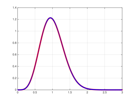
With 𝕂s±superscriptsubscript𝕂𝑠plus-or-minus\operatorname{\mathbb{K}}_{s}^{\pm} and 𝕃s±superscriptsubscript𝕃𝑠plus-or-minus\operatorname{\mathbb{L}}_{s}^{\pm} as in Proposition 5.4 we have

pξCSE(0;s)=p4,ξ(0;s)+1N2r4,ξ(0;s)+O(1N4),superscriptsubscript𝑝𝜉CSE0𝑠subscript𝑝4𝜉0𝑠1superscript𝑁2subscript𝑟4𝜉0𝑠O1superscript𝑁4p_{\xi}^{{\rm CSE}}(0;s)=p_{4,\xi}(0;s)+{1\over N^{2}}r_{4,\xi}(0;s)+\operatorname{O}\Big{(}{1\over N^{4}}\Big{)}, (5.23)

where

p4,ξ(0;s)=12ξd2ds2(det(𝕀ξ𝕂s)+det(𝕀ξ𝕂s+))subscript𝑝4𝜉0𝑠12𝜉superscript𝑑2𝑑superscript𝑠2𝕀𝜉superscriptsubscript𝕂𝑠𝕀𝜉superscriptsubscript𝕂𝑠p_{4,\xi}(0;s)={1\over 2\xi}{d^{2}\over ds^{2}}\left(\det(\operatorname{\mathbb{I}}-\xi\operatorname{\mathbb{K}}_{s}^{-})+\det(\operatorname{\mathbb{I}}-\xi\operatorname{\mathbb{K}}_{s}^{+})\right) (5.24)

and

r4,ξ(0;s)=18d2ds2(Ω(ξ𝕂s):𝕃s+Ω(ξ𝕂s+):𝕃s+).r_{4,\xi}(0;s)={1\over 8}{d^{2}\over ds^{2}}\left(\operatorname{\Omega}(\xi\operatorname{\mathbb{K}}_{s}^{-}):\operatorname{\mathbb{L}}_{s}^{-}+\operatorname{\Omega}(\xi\operatorname{\mathbb{K}}_{s}^{+}):\operatorname{\mathbb{L}}_{s}^{+}\right). (5.25)
Remark 5.7.

The case ξ=1𝜉1\xi=1 of (5.24) is due to Mehta and Dyson [34].

Refer to caption
Refer to caption
Figure 11. 00-th next neighbour spacing: simulation vs. formulae from theory for finite size CSE, no thinning (ξ=1𝜉1\xi=1). Left panel: a histogram of empirical data from CSENsubscriptCSE𝑁{\rm CSE}_{N} with N=20𝑁20N=20 scaled to unit mean spacing, computed using a bin size of 0.010.010.01 and 108superscript10810^{8} samples (blue dots); the large N𝑁N limit p4,ξ(0;s)subscript𝑝4𝜉0𝑠p_{4,\xi}(0;s) (red solid line). Right panel: the simulation data minus p4,ξ(0;s)subscript𝑝4𝜉0𝑠p_{4,\xi}(0;s) scaled by N2superscript𝑁2N^{2} (blue dots); the leading correction term r4,ξ(0,s)subscript𝑟4𝜉0𝑠r_{4,\xi}(0,s) (red solid line).
Refer to caption
Refer to caption
Figure 12. As in Figure 11 but with thinning ξ=0.6𝜉0.6\xi=0.6.

As was done for the COE, to illustrate and test the above results, we took 108superscript10810^{8} samples of CSENsubscriptCSE𝑁{\rm CSE}_{N} (N=20𝑁20N=20, again using the β=4𝛽4\beta=4 CMV sparse matrix model [30]), and from this made an empirical determination of the spacing distribution scaled to unit mean spacing. This was then subtracted from the large N𝑁N limit p4,ξ(0;s)subscript𝑝4𝜉0𝑠p_{4,\xi}(0;s) and the difference compared against r4,ξ(0;s)subscript𝑟4𝜉0𝑠r_{4,\xi}(0;s). Both ξ=1𝜉1\xi=1 (no thinning) and ξ=0.6𝜉0.6\xi=0.6 were considered; see Figures 11 and 12.

5.3. Painlevé transcendent characterisation

In addition to the integral operator characterisation of the expansion terms in Propositions 5.4 and 5.6 there is one in terms of Painlevé transcendents. Such an expression in the case of the CUE has been given in [19] and restated in (1.14)–(1.17) above. To simplify we restrict ourselves to N𝑁N being even, writing N2N𝑁2𝑁N\to 2N for definiteness. We begin by noting that the joint eigenvalue PDF for the eigen-angles {θj}subscript𝜃𝑗\{\theta_{j}\} of O±(2N+1)superscriptOplus-or-minus2𝑁1\operatorname{O}^{\pm}(2N+1) matrices in the interval (0,π)0𝜋(0,\pi), after changing variables xj=sin2(θj/2)subscript𝑥𝑗superscript2subscript𝜃𝑗2x_{j}=\sin^{2}(\theta_{j}/2), is proportional to

l=1Nxla(1xl)b1j<kN(xkxj)2,0<xl<1,superscriptsubscriptproduct𝑙1𝑁superscriptsubscript𝑥𝑙𝑎superscript1subscript𝑥𝑙𝑏subscriptproduct1𝑗𝑘𝑁superscriptsubscript𝑥𝑘subscript𝑥𝑗20subscript𝑥𝑙1\prod_{l=1}^{N}x_{l}^{a}(1-x_{l})^{b}\prod_{1\leq j<k\leq N}(x_{k}-x_{j})^{2},\qquad 0<x_{l}<1,

with a=±1/2𝑎plus-or-minus12a=\pm 1/2, b=a𝑏𝑎b=-a, which is an example of the Jacobi unitary ensemble (JUE); see e.g. [18, §3.7.1]. Hence the corresponding generating functions for the gap probabilities are related by

O±(2N+1)((0,θ);z)=JUEN((0,sin2θ2);z)|a=±1/2,b=a.superscriptsuperscriptOplus-or-minus2𝑁10𝜃𝑧evaluated-atsuperscriptsubscriptJUE𝑁0superscript2𝜃2𝑧formulae-sequence𝑎plus-or-minus12𝑏𝑎\mathcal{E}^{\operatorname{O}^{\pm}(2N+1)}((0,\theta);z)=\left.\mathcal{E}^{{\rm JUE}_{N}}\left(\left(0,\sin^{2}{\theta\over 2}\right);z\right)\right|_{a=\pm 1/2,b=-a}. (5.26)

The significance of this result for present purposes is that the RHS can be expressed as a σ𝜎\sigmaPVI transcendent [25, 22]. Specifically, reading off from [18, Eqns. (8.71), (8.75), (8.76)] we have

JUEN((0,sin2θ/2);z)=exp0sin2θ/2f±(t;z)t(t1)𝑑t,superscriptsubscriptJUE𝑁0superscript2𝜃2𝑧superscriptsubscript0superscript2𝜃2superscript𝑓plus-or-minus𝑡𝑧𝑡𝑡1differential-d𝑡\mathcal{E}^{{\rm JUE}_{N}}((0,\sin^{2}\theta/2);z)=\exp\int_{0}^{\sin^{2}\theta/2}{f^{\pm}(t;z)\over t(t-1)}\,dt, (5.27)

where f=f±𝑓superscript𝑓plus-or-minusf=f^{\pm} satisfies the particular σ𝜎\sigmaPVI equation

(t(1t)f′′)2+(fN2)(2f+(12t)f)2(f)2(fN2+14)=0,superscript𝑡1𝑡superscript𝑓′′2superscript𝑓superscript𝑁2superscript2𝑓12𝑡superscript𝑓2superscriptsuperscript𝑓2superscript𝑓superscript𝑁2140(t(1-t)f^{\prime\prime})^{2}+(f^{\prime}-N^{2})(2f+(1-2t)f^{\prime})^{2}-(f^{\prime})^{2}\Big{(}f^{\prime}-N^{2}+{1\over 4}\Big{)}=0, (5.28)

subject to the boundary condition

f±(t;z)t0+{8N(N21/4)3πzt3/2,a=1/2,2Nπzt1/2,a=1/2.superscript𝑓plus-or-minus𝑡𝑧subscriptsimilar-to𝑡superscript0cases8𝑁superscript𝑁2143𝜋𝑧superscript𝑡32𝑎122𝑁𝜋𝑧superscript𝑡12𝑎12f^{\pm}(t;z)\mathop{\sim}\limits_{t\to 0^{+}}\left\{\begin{array}[]{ll}\displaystyle{8N(N^{2}-1/4)\over 3\pi}zt^{3/2},&a=1/2,\\[5.69046pt] \displaystyle{2N\over\pi}zt^{1/2},&a=-1/2.\end{array}\right. (5.29)

We therefore have

O±(2N+1)((0,πs/N);z)=exp(0(πs)2f±(sin2u/2N;z)duNusinu/N).superscriptsuperscriptOplus-or-minus2𝑁10𝜋𝑠𝑁𝑧superscriptsubscript0superscript𝜋𝑠2superscript𝑓plus-or-minussuperscript2𝑢2𝑁𝑧𝑑𝑢𝑁𝑢𝑢𝑁\mathcal{E}^{\operatorname{O}^{\pm}(2N+1)}((0,\pi s/N);z)=\exp\Big{(}-\int_{0}^{(\pi s)^{2}}f^{\pm}(\sin^{2}\sqrt{u}/2N;z)\,{du\over N\sqrt{u}\sin\sqrt{u}/N}\Big{)}. (5.30)

To obtain an expansion consistent with (5.19) we make the ansatz

f±(sin2(w/2N);z)=f0±+f1±N2+O(N4).superscript𝑓plus-or-minussuperscript2𝑤2𝑁𝑧superscriptsubscript𝑓0plus-or-minussubscriptsuperscript𝑓plus-or-minus1superscript𝑁2Osuperscript𝑁4f^{\pm}(\sin^{2}(\sqrt{w}/2N);z)=f_{0}^{\pm}+{f^{\pm}_{1}\over N^{2}}+\operatorname{O}(N^{-4}). (5.31)

Changing variables in (5.28) t=sin2(w/2N)𝑡superscript2𝑤2𝑁t=\sin^{2}(\sqrt{w}/2N), substituting (5.31), and equating terms to leading order (N4)superscript𝑁4(N^{4}) and to next leading order (N2)superscript𝑁2(N^{2}), we obtain characterisations in terms of differential equations of f0±superscriptsubscript𝑓0plus-or-minusf_{0}^{\pm} and f1±superscriptsubscript𝑓1plus-or-minusf_{1}^{\pm}.

Proposition 5.8.

The leading function f0±superscriptsubscript𝑓0plus-or-minusf_{0}^{\pm} in (5.31) satisfies the particular σPIII𝜎superscriptPIII\sigma{\rm PIII}^{\prime} equation (with v1=v2=1/2subscript𝑣1subscript𝑣212v_{1}=v_{2}=1/2 in the notation of [18, Eq. (8.15)])

w2(f0′′)2(f0)24+4f0(f0)2+w(f0)24w(f0)3f0f0=0,superscript𝑤2superscriptsuperscriptsubscript𝑓0′′2superscriptsuperscriptsubscript𝑓0244subscript𝑓0superscriptsuperscriptsubscript𝑓02𝑤superscriptsuperscriptsubscript𝑓024𝑤superscriptsuperscriptsubscript𝑓03subscript𝑓0superscriptsubscript𝑓00w^{2}(f_{0}^{\prime\prime})^{2}-{(f_{0}^{\prime})^{2}\over 4}+4f_{0}(f_{0}^{\prime})^{2}+w(f_{0}^{\prime})^{2}-4w(f_{0}^{\prime})^{3}-f_{0}f_{0}^{\prime}=0, (5.32)

subject to the boundary condition

f0ν(w;z){z3πw3/2,ν=+,zπw1/2,ν=.similar-tosuperscriptsubscript𝑓0𝜈𝑤𝑧cases𝑧3𝜋superscript𝑤32𝜈𝑧𝜋superscript𝑤12𝜈f_{0}^{\nu}(w;z)\sim\left\{\begin{array}[]{ll}\displaystyle{z\over 3\pi}w^{3/2},&\nu=+,\\[11.38092pt] \displaystyle{z\over\pi}w^{1/2},&\nu=-.\end{array}\right. (5.33)

The function f1±subscriptsuperscript𝑓plus-or-minus1f^{\pm}_{1} in (5.31) satisfies the second order linear differential equation

A1(w;z)f1′′+B1(w;z)f1+C1(w;z)f1+D1(w;z)=0,subscript𝐴1𝑤𝑧superscriptsubscript𝑓1′′subscript𝐵1𝑤𝑧superscriptsubscript𝑓1subscript𝐶1𝑤𝑧subscript𝑓1subscript𝐷1𝑤𝑧0A_{1}(w;z)f_{1}^{\prime\prime}+B_{1}(w;z)f_{1}^{\prime}+C_{1}(w;z)f_{1}+D_{1}(w;z)=0, (5.34)

where the coefficients are given in terms of f0=f0±subscript𝑓0superscriptsubscript𝑓0plus-or-minusf_{0}=f_{0}^{\pm} according to

A1(w;z)subscript𝐴1𝑤𝑧\displaystyle A_{1}(w;z) =2w2f0′′,absent2superscript𝑤2superscriptsubscript𝑓0′′\displaystyle=2w^{2}f_{0}^{\prime\prime},
B1(w;z)subscript𝐵1𝑤𝑧\displaystyle B_{1}(w;z) =8f0f0+2wf012wf02f0f02,absent8subscript𝑓0superscriptsubscript𝑓02𝑤superscriptsubscript𝑓012𝑤superscriptsubscript𝑓02subscript𝑓0superscriptsubscript𝑓02\displaystyle=8f_{0}f_{0}^{\prime}+2wf_{0}^{\prime}-12wf_{0}^{2}-f_{0}-{f_{0}^{\prime}\over 2},
C1(w;z)subscript𝐶1𝑤𝑧\displaystyle C_{1}(w;z) =f0(4f01),absentsuperscriptsubscript𝑓04superscriptsubscript𝑓01\displaystyle=f_{0}^{\prime}(4f_{0}^{\prime}-1),
D1(w;z)subscript𝐷1𝑤𝑧\displaystyle D_{1}(w;z) =f03(3f02+w2f0′′2w2(f0)2+wf0wf042wf0f0)f024,absentsuperscriptsubscript𝑓033superscriptsubscript𝑓02superscript𝑤2superscriptsubscript𝑓0′′2superscript𝑤2superscriptsuperscriptsubscript𝑓02𝑤subscript𝑓0𝑤superscriptsubscript𝑓042𝑤subscript𝑓0superscriptsubscript𝑓0superscriptsubscript𝑓024\displaystyle={f_{0}^{\prime}\over 3}\Big{(}3f_{0}^{2}+w^{2}f_{0}^{\prime\prime}-2w^{2}(f_{0}^{\prime})^{2}+wf_{0}-{wf_{0}^{\prime}\over 4}-2wf_{0}f_{0}^{\prime}\Big{)}-{f_{0}^{2}\over 4},

subject to the boundary condition

f1±(w;z)zw3/212π,similar-tosuperscriptsubscript𝑓1plus-or-minus𝑤𝑧𝑧superscript𝑤3212𝜋f_{1}^{\pm}(w;z)\sim-{zw^{3/2}\over 12\pi}, (5.35)

which is thus the same in both cases. In terms of f0±superscriptsubscript𝑓0plus-or-minusf_{0}^{\pm} and f1±superscriptsubscript𝑓1plus-or-minusf_{1}^{\pm} we have

O±(2N+1)((0,πs/N);z)=exp(0(πs)2f0±(w;z)w𝑑w)×(11N20(πs)2wf0±(w;z)+6f1±(w;z)6w𝑑w+O(1N4)).superscriptsuperscriptOplus-or-minus2𝑁10𝜋𝑠𝑁𝑧superscriptsubscript0superscript𝜋𝑠2superscriptsubscript𝑓0plus-or-minus𝑤𝑧𝑤differential-d𝑤11superscript𝑁2superscriptsubscript0superscript𝜋𝑠2𝑤superscriptsubscript𝑓0plus-or-minus𝑤𝑧6superscriptsubscript𝑓1plus-or-minus𝑤𝑧6𝑤differential-d𝑤O1superscript𝑁4\mathcal{E}^{\operatorname{O}^{\pm}(2N+1)}((0,\pi s/N);z)=\exp\left(-\int_{0}^{(\pi s)^{2}}{f_{0}^{\pm}(w;z)\over w}\,dw\right)\\ \times\left(1-{1\over N^{2}}\int_{0}^{(\pi s)^{2}}{wf_{0}^{\pm}(w;z)+6f_{1}^{\pm}(w;z)\over 6w}\,dw+\operatorname{O}\Big{(}{1\over N^{4}}\Big{)}\right). (5.36)
Remark 5.9.

A problem for future study is to describe how the solutions of (1.15) and (5.34) relate to the broader Painlevé theory.777This was raised by one of the referees.

Scaling the eigen-angles of COE2NsubscriptCOE2𝑁{\rm COE}_{2N} to have unit mean spacing by setting θ=πs/N𝜃𝜋𝑠𝑁\theta=\pi s/N, we can now substitute (5.36) into (5.7); then—after using (3.13) to add the presence of thinning—substitute the result in (5.18) and compare with (5.19) to obtain characterisations of the expansion terms p1,ξ(0;s)subscript𝑝1𝜉0𝑠p_{1,\xi}(0;s) and r1,ξ(0;s)subscript𝑟1𝜉0𝑠r_{1,\xi}(0;s) in terms of Painlevé transcendents.

Proposition 5.10.

We have

p1,ξ(0;s)=1ξ(2ξ)d2ds2((1ξ)exp(0(πs/2)2f0+(w;2ξξ2)wdw)+exp(0(πs/2)2f0(w;2ξξ2)wdw))subscript𝑝1𝜉0𝑠1𝜉2𝜉superscript𝑑2𝑑superscript𝑠21𝜉superscriptsubscript0superscript𝜋𝑠22superscriptsubscript𝑓0𝑤2𝜉superscript𝜉2𝑤𝑑𝑤superscriptsubscript0superscript𝜋𝑠22superscriptsubscript𝑓0𝑤2𝜉superscript𝜉2𝑤𝑑𝑤p_{1,\xi}(0;s)={1\over\xi(2-\xi)}{d^{2}\over ds^{2}}\left((1-\xi)\exp\left(-\int_{0}^{(\pi s/2)^{2}}{f_{0}^{+}(w;2\xi-\xi^{2})\over w}\,dw\right)\right.\\ \left.+\exp\left(-\int_{0}^{(\pi s/2)^{2}}{f_{0}^{-}(w;2\xi-\xi^{2})\over w}\,dw\right)\right) (5.37)

and

r1,ξ(0;s)=4ξ(2ξ)d2ds2((1ξ)0(πs/2)2wf0+(w;2ξξ2)+6f1+(w;2ξξ2)6wdw×exp(0(πs/2)2f0+(w;2ξξ2)w𝑑w)+0(πs/2)2wf0(w;2ξξ2)+6f1(w;2ξξ2)6w𝑑w×exp(0(πs/2)2f0(w;2ξξ2)wdw)).subscript𝑟1𝜉0𝑠4𝜉2𝜉superscript𝑑2𝑑superscript𝑠21𝜉superscriptsubscript0superscript𝜋𝑠22𝑤superscriptsubscript𝑓0𝑤2𝜉superscript𝜉26superscriptsubscript𝑓1𝑤2𝜉superscript𝜉26𝑤𝑑𝑤superscriptsubscript0superscript𝜋𝑠22superscriptsubscript𝑓0𝑤2𝜉superscript𝜉2𝑤differential-d𝑤superscriptsubscript0superscript𝜋𝑠22𝑤superscriptsubscript𝑓0𝑤2𝜉superscript𝜉26superscriptsubscript𝑓1𝑤2𝜉superscript𝜉26𝑤differential-d𝑤superscriptsubscript0superscript𝜋𝑠22superscriptsubscript𝑓0𝑤2𝜉superscript𝜉2𝑤𝑑𝑤r_{1,\xi}(0;s)=\\ -{4\over\xi(2-\xi)}{d^{2}\over ds^{2}}\left((1-\xi)\int_{0}^{(\pi s/2)^{2}}{wf_{0}^{+}(w;2\xi-\xi^{2})+6f_{1}^{+}(w;2\xi-\xi^{2})\over 6w}\,dw\right.\\ \times\exp\left(-\int_{0}^{(\pi s/2)^{2}}{f_{0}^{+}(w;2\xi-\xi^{2})\over w}\,dw\right)\\ \quad+\int_{0}^{(\pi s/2)^{2}}{wf_{0}^{-}(w;2\xi-\xi^{2})+6f_{1}^{-}(w;2\xi-\xi^{2})\over 6w}\,dw\\ \left.\times\exp\left(-\int_{0}^{(\pi s/2)^{2}}{f_{0}^{-}(w;2\xi-\xi^{2})\over w}\,dw\right)\right). (5.38)
Remark 5.11.

The case ξ=1𝜉1\xi=1 of (5.37) agrees with the σPIII𝜎superscriptPIII\sigma{\rm PIII}^{\prime} formula for p1(0;s)subscript𝑝10𝑠p_{1}(0;s) (no thinning) reported in [21] and [17].

The differential equations (5.32) and (5.34) can be used to successively generate terms in the series expansions of f0±superscriptsubscript𝑓0plus-or-minusf_{0}^{\pm} and f1±superscriptsubscript𝑓1plus-or-minusf_{1}^{\pm} about the origin, extending the boundary conditions (5.33) and (5.35). Substituting these into (5.37) and (5.38) then provides us with the small s𝑠s expansion of p1,ξ(0;s)subscript𝑝1𝜉0𝑠p_{1,\xi}(0;s) and r1,ξ(0;s)subscript𝑟1𝜉0𝑠r_{1,\xi}(0;s).

Corollary 5.12.

We have

p1,ξ(0;s)=16π2ξs160π4ξs31270π4(ξ2)ξs4+π6ξs51680+π6(ξ2)ξs64725π8ξs790720+π8(ξ2)(3ξ32)ξs85292000+π10ξs97983360+O(s10)subscript𝑝1𝜉0𝑠16superscript𝜋2𝜉𝑠160superscript𝜋4𝜉superscript𝑠31270superscript𝜋4𝜉2𝜉superscript𝑠4superscript𝜋6𝜉superscript𝑠51680superscript𝜋6𝜉2𝜉superscript𝑠64725superscript𝜋8𝜉superscript𝑠790720superscript𝜋8𝜉23𝜉32𝜉superscript𝑠85292000superscript𝜋10𝜉superscript𝑠97983360Osuperscript𝑠10p_{1,\xi}(0;s)=\frac{1}{6}\pi^{2}\xi s-\frac{1}{60}\pi^{4}\xi s^{3}-\frac{1}{270}\pi^{4}(\xi-2)\xi s^{4}+\frac{\pi^{6}\xi s^{5}}{1680}+\frac{\pi^{6}(\xi-2)\xi s^{6}}{4725}\\[5.69054pt] -\frac{\pi^{8}\xi s^{7}}{90720}+\frac{\pi^{8}(\xi-2)(3\xi-32)\xi s^{8}}{5292000}+\frac{\pi^{10}\xi s^{9}}{7983360}+\operatorname{O}(s^{10}) (5.39)

and

r1,ξ(0;s)=16π2ξs+118π4ξs3+154π4(ξ2)ξs41240π6ξs54π6(ξ2)ξs62025+π8ξs77560π8(ξ2)(3ξ32)ξs8352800π10ξs9435456+O(s10).subscript𝑟1𝜉0𝑠16superscript𝜋2𝜉𝑠118superscript𝜋4𝜉superscript𝑠3154superscript𝜋4𝜉2𝜉superscript𝑠41240superscript𝜋6𝜉superscript𝑠54superscript𝜋6𝜉2𝜉superscript𝑠62025superscript𝜋8𝜉superscript𝑠77560superscript𝜋8𝜉23𝜉32𝜉superscript𝑠8352800superscript𝜋10𝜉superscript𝑠9435456Osuperscript𝑠10r_{1,\xi}(0;s)=-\frac{1}{6}\pi^{2}\xi s+\frac{1}{18}\pi^{4}\xi s^{3}+\frac{1}{54}\pi^{4}(\xi-2)\xi s^{4}-\frac{1}{240}\pi^{6}\xi s^{5}-\frac{4\pi^{6}(\xi-2)\xi s^{6}}{2025}\\[5.69054pt] +\frac{\pi^{8}\xi s^{7}}{7560}-\frac{\pi^{8}(\xi-2)\left(3\xi-32\right)\xi s^{8}}{352800}-\frac{\pi^{10}\xi s^{9}}{435456}+\operatorname{O}\left(s^{10}\right). (5.40)

We remark that setting ξ=1𝜉1\xi=1 in (5.39) extends the expansion of p1,ξ(0;s)|ξ=1evaluated-atsubscript𝑝1𝜉0𝑠𝜉1p_{1,\xi}(0;s)|_{\xi=1} given in [18, Eq. (8.141)].

For the analogous results in the case of the CSENsubscriptCSE𝑁{\rm CSE}_{N}, scaling the eigen-angles to have unit mean spacing by setting θ=2πs/N𝜃2𝜋𝑠𝑁\theta=2\pi s/N, we substitute (5.36) into (5.16); then—after using (3.13) to add the presence of thinning—substitute the result in (5.22) and compare with (5.23).

Proposition 5.13.

We have

p4,ξ(0;s)=12ξd2ds2(exp(0(πs)2f0+(w;ξ)w𝑑w)+exp(0(πs)2f0(w;ξ)w𝑑w))subscript𝑝4𝜉0𝑠12𝜉superscript𝑑2𝑑superscript𝑠2superscriptsubscript0superscript𝜋𝑠2superscriptsubscript𝑓0𝑤𝜉𝑤differential-d𝑤superscriptsubscript0superscript𝜋𝑠2superscriptsubscript𝑓0𝑤𝜉𝑤differential-d𝑤p_{4,\xi}(0;s)\\ ={1\over 2\xi}{d^{2}\over ds^{2}}\left(\exp\left(-\int_{0}^{(\pi s)^{2}}{f_{0}^{+}(w;\xi)\over w}\,dw\right)+\exp\left(-\int_{0}^{(\pi s)^{2}}{f_{0}^{-}(w;\xi)\over w}\,dw\right)\right) (5.41)

and

r4,ξ(0;s)=12ξd2ds2((0(πs)2wf0+(w;ξ)+6f1+(w;ξ)6wdw)×exp(0(πs)2f0+(w;ξ)w𝑑w)+(0(πs)2wf0(w;ξ)+6f1(w;ξ)6wdw)exp(0(πs)2f0(w;ξ)wdw)).subscript𝑟4𝜉0𝑠12𝜉superscript𝑑2𝑑superscript𝑠2superscriptsubscript0superscript𝜋𝑠2𝑤superscriptsubscript𝑓0𝑤𝜉6superscriptsubscript𝑓1𝑤𝜉6𝑤𝑑𝑤superscriptsubscript0superscript𝜋𝑠2superscriptsubscript𝑓0𝑤𝜉𝑤differential-d𝑤superscriptsubscript0superscript𝜋𝑠2𝑤superscriptsubscript𝑓0𝑤𝜉6superscriptsubscript𝑓1𝑤𝜉6𝑤𝑑𝑤superscriptsubscript0superscript𝜋𝑠2superscriptsubscript𝑓0𝑤𝜉𝑤𝑑𝑤r_{4,\xi}(0;s)=-{1\over 2\xi}{d^{2}\over ds^{2}}\left(\left(\int_{0}^{(\pi s)^{2}}{wf_{0}^{+}(w;\xi)+6f_{1}^{+}(w;\xi)\over 6w}\,dw\right)\right.\\ \times\exp\left(-\int_{0}^{(\pi s)^{2}}{f_{0}^{+}(w;\xi)\over w}\,dw\right)\\ \quad\left.+\left(\int_{0}^{(\pi s)^{2}}{wf_{0}^{-}(w;\xi)+6f_{1}^{-}(w;\xi)\over 6w}\,dw\right)\exp\left(-\int_{0}^{(\pi s)^{2}}{f_{0}^{-}(w;\xi)\over w}\,dw\right)\right). (5.42)
Remark 5.14.

As in Remark 5.11 the case ξ=1𝜉1\xi=1 of (5.41) agrees with the σPIII𝜎superscriptPIII\sigma\text{PIII}^{\prime} formula for p4(0;s)subscript𝑝40𝑠p_{4}(0;s) (no thinning) reported in [21] and [17].

As with Corollary 5.12 we can use these characterisations to generate power series expansions about the origin.

Corollary 5.15.

We have

p4,ξ(0;s)subscript𝑝4𝜉0𝑠\displaystyle p_{4,\xi}(0;s) =16135π4ξs4128π6ξs64725+512π8ξs816537534816π10ξs10147349125+O(s12),absent16135superscript𝜋4𝜉superscript𝑠4128superscript𝜋6𝜉superscript𝑠64725512superscript𝜋8𝜉superscript𝑠816537534816superscript𝜋10𝜉superscript𝑠10147349125Osuperscript𝑠12\displaystyle=\frac{16}{135}\pi^{4}\xi s^{4}-\frac{128\pi^{6}\xi s^{6}}{4725}+\frac{512\pi^{8}\xi s^{8}}{165375}-\frac{34816\pi^{10}\xi s^{10}}{147349125}+\operatorname{O}(s^{12}),
r4,ξ(0;s)subscript𝑟4𝜉0𝑠\displaystyle r_{4,\xi}(0;s) =427π4ξs4+128π6ξs62025128π8ξs811025+17408π10ξs1013395375+O(s12).absent427superscript𝜋4𝜉superscript𝑠4128superscript𝜋6𝜉superscript𝑠62025128superscript𝜋8𝜉superscript𝑠81102517408superscript𝜋10𝜉superscript𝑠1013395375Osuperscript𝑠12\displaystyle=-\frac{4}{27}\pi^{4}\xi s^{4}+\frac{128\pi^{6}\xi s^{6}}{2025}-\frac{128\pi^{8}\xi s^{8}}{11025}+\frac{17408\pi^{10}\xi s^{10}}{13395375}+\operatorname{O}(s^{12}).

Appendix: Implementation

The method of Section 2.2 for numerically evaluating general terms of integral operators is most easily added to the Matlab toolbox described in [10]; the basic code needed to run it is as follows:

1function [val,err,n] = OperatorTerm(term,varargin)
2
3%OPERATORTERM evaluates terms of integral operators that have a scalar value.
4%
5%OPERATORTERM(term,K1,...,Km) returns the value of the
6%expression ’term(K1,...,Km)’ for m discrete integral
7%operators K1,...,Km (that is, for Nyström matrices of
8%a variable dimension n, which is chosen adaptively).
9%The value to be returned must be scalar.
10
11tol = 5e-15;
12n = 7; n_max = 1000;
13
14operators = cell(size(varargin));
15
16val0 = inf;
17while n < n_max
18 n = floor(1.41*n);
19 for k = 1:length(varargin)
20 operators{k} = varargin{k}(n);
21 end
22 val = term(operators{:});
23 err = abs(val-val0);
24 if err < tol; break; end
25 val0 = val;
26end

From the user perspective this command is called with a considerable symbolic look and feel. For example, the leading order term in (1.11), that is,

det(𝕀𝕂s)𝕀subscript𝕂𝑠\det(\operatorname{\mathbb{I}}-\operatorname{\mathbb{K}}_{s})

evaluates for s=1𝑠1s=1 to the following value:

1s = 1;
2K = op(@(x,y) sinc(pi*(x-y)),[0,s]);
3I = @(K) eye(size(K));
4lead = @(K) det(I(K) - K);
5[val,err,n] = OperatorTerm(lead,K);
6PrintCorrectDigits(val,err);
7
8 0.170217421379185

and the leading correction term in (1.11), that is,

Ω(𝕂s):𝕃s=det(𝕀𝕂s)tr((𝕀𝕂s)1𝕃s),:Ωsubscript𝕂𝑠subscript𝕃𝑠𝕀subscript𝕂𝑠trsuperscript𝕀subscript𝕂𝑠1subscript𝕃𝑠\operatorname{\Omega}(\operatorname{\mathbb{K}}_{s}):\operatorname{\mathbb{L}}_{s}=-\det(\operatorname{\mathbb{I}}-\operatorname{\mathbb{K}}_{s})\operatorname{tr}\left((\operatorname{\mathbb{I}}-\operatorname{\mathbb{K}}_{s})^{-1}\operatorname{\mathbb{L}}_{s}\right),

evaluates for s=1𝑠1s=1 to the following value:

9L = op(@(x,y) pi*(x-y).*sin(pi*(x-y))/6,[0,s]);
10corr = @(K,L) -det(I(K)-K)*trace((I(K)-K)\L);
11[val,err,n] = OperatorTerm(corr,K,L);
12PrintCorrectDigits(val,err);
13
14 -0.075241982465122

Since the estimated error has been taken into account when printing these values, they are good to about 15 digits; in both cases the adaptively chosen number of Gauss–Legendre quadrature points (that is, the dimension of the Nyström matrices representing the integral operators) was as small as n=15𝑛15n=15, which is a clear sign of the exponential convergence of the method. CPU time is about a millisecond.

Acknowledgements

We are grateful to A. Odlyzko for providing us with the Riemann zero data set. We would also like to thank the referees for their thoughtful comments. The research of F.B. was supported by the DFG-Collaborative Research Center, TRR 109, “Discretization in Geometry and Dynamics.” The research of P.J.F. and A.M. is part of the program of study supported by the ARC Centre of Excellence for Mathematical & Statistical Frontiers.

References

  • [1] A. Altland and M.R. Zirnbauer, Nonstandard symmetry classes in mesoscopic normal-superconducting hybrid compounds, Phys. Rev. B 55 (1997), 1142–1161.
  • [2] J. Baik and E.M. Rains, Algebraic aspects of increasing subsequences, Duke Math. J. 109 (2001), 1–65.
  • [3] M.V. Berry and J.P. Keating, The Riemann zeros and eigenvalue asymptotics, SIAM Rev. 41 (1999), 236–266.
  • [4] I. Bogaert, Iteration-free computation of Gauss-Legendre quadrature nodes and weights, SIAM J. Sci. Comput. 36 (2014), A1008-A1026.
  • [5] E. Bogomolny, O. Bohigas, P. Leboeuf, and A.C. Monastra, On the spacing distribution of the Riemann zeros: corrections to the asymptotic result, J. Phys. A 39 (2006), 10743–10754.
  • [6] E. Bogomolny and J.P. Keating, Gutzwiller’s trace formula and spectral statistics: beyond the diagonal approximation, Phys. Rev. Lett. 77 (1996), 1472–1475.
  • [7] by same author, A method for calculating spectral statistics based on random-matrix universality with an application to the three-point correlations of the Riemann zeros, J. Phys. A 46 (2013), 305203, 17pp.
  • [8] O. Bohigas, M.J. Giannoni, and C. Schmit, Characterization of chaotic quantum spectra and universality of level fluctuation laws, Phys. Rev. Lett. 52 (1984), 1–4.
  • [9] O. Bohigas and M.P. Pato, Missing levels in correlated spectra, Phys. Lett. B 595 (2004), 171–176.
  • [10] F. Bornemann, On the numerical evaluation of distributions in random matrix theory: a review, Markov Processes Relat. Fields 16 (2010), 803–866.
  • [11] by same author, On the numerical evaluation of Fredholm determinants, Math. Comp. 79 (2010), 871–915.
  • [12] F. Bornemann and P.J. Forrester, Singular values and evenness symmetry in random matrix theory, Forum Math. DOI: 10.1515/forum-2015-0055 (2015), 19pp.
  • [13] F.J. Dyson, Statistical theory of energy levels of complex systems II, J. Math. Phys. 3 (1962), 157–165.
  • [14] by same author, Statistical theory of energy levels of complex systems III, J. Math. Phys. 3 (1962), 166–175.
  • [15] by same author, The three fold way. Algebraic structure of symmetry groups and ensembles in quantum mechanics, J. Math. Phys. 3 (1962), 1199–1215.
  • [16] F.W.K. Firk and S.J. Miller, Nuclei, primes and the random matrix connection, Symmetry 1 (2009), 64–105.
  • [17] P.J. Forrester, Evenness symmetry and inter-relationships between gap probabilities in random matrix theory, Forum Math. 18 (2006), 711–743.
  • [18] by same author, Log-gases and random matrices, Princeton University Press, Princeton, NJ, 2010.
  • [19] P.J. Forrester and A. Mays, Finite-size corrections in random matrix theory and Odlyzko’s dataset for the Riemann zeros, Proc. Roy. Soc. A 471 (2015), 20150436, 21pp.
  • [20] P.J. Forrester and A.M. Odlyzko, Gaussian unitary ensemble eigenvalues and Riemann ζ𝜁\zeta function zeros: a non-linear equation for a new statistic, Phys. Rev. E 54 (1996), R4493–R4495.
  • [21] P.J. Forrester and N.S. Witte, Exact Wigner surmise type evaluation of the spacing distribution in the bulk of the scaled random matrix ensembles, Lett. Math. Phys. 53 (2000), 195–200.
  • [22] by same author, Application of the τ𝜏\tau-function theory of Painlevé equations to random matrices: PVI, the JUE,CyUE, cJUE and scaled limits, Nagoya Math. J. 174 (2004), 29–114.
  • [23] M. Gaudin, Sur la loi limite de l’espacement des valeurs propres d’une matrice aléatoire, Nucl. Phys. 25 (1961), 447–458.
  • [24] J. Gunson, Proof of a conjecture of Dyson in the statistical theory of energy levels, J. Math. Phys. 4 (1962), 752–753.
  • [25] L. Haine and J.-P. Semengue, The Jacobi polynomial ensemble and the Painlevé VI equation, J. Math. Phys. 40 (1999), 2117–2134.
  • [26] J. Illian, A. Penttinen, H. Stoyan, and D. Stoyan, Statistical analysis and modelling of spatial point patterns, Wiley, 2008.
  • [27] M. Jimbo, T. Miwa, Y. Môri, and M. Sato, Density matrix of an impenetrable Bose gas and the fifth Painlevé transcendent, Physica 1D (1980), 80–158.
  • [28] N.M. Katz and P. Sarnak, Zeroes of zeta functions and symmetry, Bull. Amer. Math. Soc. 36 (1999), 1–26.
  • [29] J.P. Keating and N.C. Snaith, Random matrix theory and ζ(1/2+it)𝜁12𝑖𝑡\zeta(1/2+it), Commun. Math. Phys. 214 (2001), 57–89.
  • [30] R. Killip and I. Nenciu, Matrix models for circular ensembles, Int. Math. Res. Not. 50 (2004), 2665–2701.
  • [31] R.J. Mathar, Series of reciprocal powers of k𝑘k-almost primes (2009), arXiv:0803.0900v3.
  • [32] M.L. Mehta, On the statistical properties of the level-spacings in nuclear spectra, Nucl. Phys. B 18 (1960), 395–419.
  • [33] by same author, Power series for level spacing functions of random matrix ensembles, Z. Phys. B 86 (1992), 285–290.
  • [34] M.L. Mehta and F.J. Dyson, Statistical theory of the energy levels of complex systems. V, J. Math. Phys. 4 (1963), 713–719.
  • [35] A.M. Odlyzko, On the distribution of spacings between zeros of the zeta function, Math. Comput. 48 (1987), 273–308.
  • [36] by same author, The 1022superscript102210^{22}-nd zero of the Riemann zeta function, Dynamical, Spectral, and Arithmeitc Zeta Functions (M. van Frankenhuysen and M.L. Lapidus, eds.), Contemporary Math., vol. 290BB, Amer. Math. Soc, Providence, RI, 2001, pp. 139–144.
  • [37] G. Sierra and J. Rodriguez-Laguna, H=xp𝐻𝑥𝑝H=xp model revisited and the Riemann zeros, Phys. Rev. Lett. 106 (2011), 200201.
  • [38] B. Simon, Trace ideals and their applications, 2nd ed., American Mathematical Society, Providence, 2005.
  • [39] H.-J. Stöckmann, Microwave billiards and quantum chaos, Scholarpedia, 5(10) (2010), 10243.
  • [40] E.P. Wigner, Gatlinburg conference on neutron physics, Oak Ridge National Laboratory Report ORNL 2309 (1957), 59.
  • [41] Wikipedia, Hilbert–Pólya conjecture, en.wikipedia.org/wiki/Hilbert-Pólya_conjecture.