e-asaleksander.stachowski@uj.edu.pl \thankstexte-msmarek.szydlowski@uj.edu.pl \thankstexte-abandrzej.borowiec@ift.uni.wroc.pl
Starobinsky cosmological model in Palatini formalism
Abstract
We classify singularities in FRW cosmologies, which dynamics can be reduced to the dynamical system of the Newtonian type. This classification is performed in terms of geometry of a potential function if it has poles. At the sewn singularity, which is of a finite scale factor type, the singularity in the past meets the singularity in the future. We show, that such singularities appear in the Starobinsky model in in the Palatini formalism, when dynamics is determined by the corresponding piece-wise smooth dynamical system. As an effect we obtain a degenerated singularity. Analytical calculations are given for the cosmological model with matter and the cosmological constant. The dynamics of model is also studied using dynamical system methods. From the phase portraits we find generic evolutionary scenarios of the evolution of the Universe. For this model, the best fit value of is equal . We consider model in both Jordan and Einstein frames. We show that after transition to the Einstein frame we obtain both form of the potential of the scalar field and the decaying Lambda term.
1 Introduction
The main aim of the paper is the construction of the Starobinsky model with a squared term in the Palatini formalism and the investigation of cosmological implications of this model. In this model the inflation phase of evolution of the universe can be obtained by the modification of general relativity in the framework of modified gravity theories DeFelice:2010aj . In this context, historically the first theory of inflation was proposed by Starobinsky Starobinsky:1980te . In the original Starobinsky model the term was motivated by the conformal anomaly in the quantum gravity. Problem of inflation in cosmological model are strictly related with the choice of frames. Authors DeFelice:2010aj show that CMB spectra in the both Einstein and Jordan frames are different functions of the number of e-foldings until the end of inflation.
Inflation is a hypothesis about the existence of a short but very fast (of exponential type) accelerated growth of the scale factor during the early evolution of the universe, after the Big-Bang but before the radiation-dominated epoch Guth:1980zm ; Linde:1986fd . It implies . Irregularities in the early epoch may lead to the formation of structures in the Universe due to the appearance of inflation.
Starobinsky Starobinsky:1980te was the first who proposed a very simple theoretical model with one parameter (energy scale ) of such inflation and which is in a good agreement with astronomical data and CMB observation. The Starobinsky model is representing the simplest version of gravity theories which have been developed considerably in the last decade Nojiri:2006ri ; DeFelice:2010aj ; Sotiriou:2008rp , whose extra term in the Lagrangian is quadratic in the scalar curvature. This model predicts the value of spectral index , at the 68% CL, with deviation from scale-invariance of the primordial power spectrum Mukhanov:1981xt ; Starobinsky:1983zz
The Starobinsky model is also compatible with Planck 2015 data Ade:2015rim and nicely predicts the number e-folds between the start and end of inflation Cheng:2013iya .
It has been recently investigated some generalization of the Starobinsky inflationary model with a polynomial form of . It was demonstrated that the slow-roll inflation can be achieved as long as the dimensionless coupling is sufficiently small Huang:2013hsb .
The Starobinsky model becomes generic because the smallness of the dimensionless coupling constant does not imply that fine-tuning is necessary Huang:2013hsb . The Starobinsky model was developed in many papers Starobinsky:1983zz ; Kofman:1985aw ; Ketov:2010qz ; Appleby:2009uf ; Capozziello:2009hc ; Alho:2016gzi ; Capozziello:2015wsa .
In this paper we develop the idea of endogenous inflation as an effect of modification of the FRW equation after the formulation of cosmological model in the Palatini formalism.
We are looking for an inflation mechanism as a pure dynamical mechanism driven by presence of the additional term (square of the Ricci scalar) in the Lagrangian, without necessity of the choice of a frame (Einstein vs Jordan frame) Alho:2016gzi ; Capozziello:2015wsa ; Capozziello:2010sc .
In the modern cosmology, the most popular trend is to explain the dark energy and the dark matter in terms of some substances, which nature is unknown up to now. Albert Einstein was representing the opposite relational point of view on description of gravity, in which all substantial forms should be eliminated. Such a point of view is called anti-substantialism. Extended gravity models Sotiriou:2008rp ; Carroll:2004de offer intrinsic or geometric models of both dark matter and dark energy—the key elements of Standard Cosmological Model. Therefore, the Einstein idea of relational gravity, in which dark matter and dark energy can be interpreted as geometric objects, is naturally realized in extended gravity. The methods of dynamical system in the context of investigation dynamics of models are used since Carroll Carroll:2004de ; Borowiec:2011wd .
Unfortunately, the metric formulation of extended gravity gives rise to fourth order field equations. To avoid this difficulty, the Palatini formalism can be apply where both the metric and symmetric connection are assumed to be independent dynamical variables. In consequence, one gets a system of second order partial differential equations. The Palatini approach reveals that the early universe inherits properties of the global CDM evolution.
In the Palatini gravity action for gravity is introduced to be
| (1) |
where is the generalized Ricci scalar and is the Ricci tensor of a torsionless connection . In this paper, we assume that . The equation of motion obtained from the first order Palatini formalism reduces to
| (2) |
| (3) |
where is matter energy momentum tensor, i.e. one assumes that the matter minimally couples to the metric. As a consequence the energy momentum tensor is conserved, i.e.: Koivisto:2005yk . In eq. (3) means the covariant derivative calculated with respect to . In order to solve equation (3) it is convenient to introduce a new metric
| (4) |
for which the connection is a Levi-Civita connection. As a consequence in dim one gets
| (5) |
i.e. that both metrics are related by the conformal factor. For this reason one should assume that the conformal factor , so it has strictly positive or negative values.
Taking the trace of (2), we obtain additional so called structural equation
| (6) |
where . Because of cosmological applications we assume that the metric is FRW metric
| (7) |
where is the scale factor, is a constant of spatial curvature (), is the cosmological time. For simplicity of presentation we consider the flat model ().
As a source of gravity we assume perfect fluid with the energy-momentum tensor
| (8) |
where , is a form of the equation of state ( for dust and for radiation). Formally, effects of the spatial curvature can be also included to the model by introducing a curvature fluid , with the barotropic factor (). From the conservation condition we obtain that . Therefore trace reads as
| (9) |
In what follows we consider visible and dark matter in the form of dust , dark energy with and radiation with .
Because a form of the function is unknown, one needs to probe it via ensuing cosmological models. Here we choose the simplest modification of the general relativity Lagrangian
| (10) |
induced by first three terms in the power series decomposition of an arbitrary function . In fact, since the terms have different physical dimensions, i.e. for , one should take instead the function for constructing our Lagrangian, where is a constant and . In this case the power series expansion reads: , where the coefficients are dimensionless, while are dimension full.
From the other hand the Lagrangian (10) can be viewed as a simplest deviation, by the quadratic Starobinsky term, from the Lagrangian which provides the standard cosmological model a.k.a. CDM model. A corresponding solution of the structural equation (6)
| (11) |
is, in fact, exactly the same as for the CDM model, i.e. with . However, the Friedmann equation of the CDM model (with dust matter, dark energy and radiation)
| (12) |
is now hardly affected by the presence of quadratic term. More exactly a counterpart of the above formula in the model under consideration looks as follows
| (13) |
where
| (14) | ||||
| (15) | ||||
| (16) | ||||
| (17) | ||||
| (18) | ||||
| (19) | ||||
| (20) | ||||
| (21) |
From the above one can check that the standard model (12) can be reconstructed in the limit . The study of this generalized Friedmann equation is a main subject of our research.
The paper is organized as follows. In section 2, we consider the Palatini approach in the Jordan and Einstein frame. In section 3, we present some generalities concerning dynamical systems of Newtonian type, and their relations with the Palatini-Starobinsky model. Section 4, is devoted to classification of cosmological singularities with special attention on Newtonian type systems represented by potential function . We adopt the Fernandes-Jambrina and Lazkoz classification of singularities FernandezJambrina:2006hj to these systems using the notion of elasticity of the potential function with respect the scale factor. In section 5, we will analyze the singularities in the Starobinsky model in the Palatini formalism. This system requires the form of piece-wise smooth dynamical system. Statistical analysis of the model is presented in section 6. In section 7, we shall summarize obtained results and draw some conclusions.
2 The Palatini approach in different frames (Jordan vs Einstein frame)
Because the effect of acceleration can depend on a choice of a frame Bahamonde:2017kbs this section is devoted to showing the existence of the inflation effect if the model is considered in the Einstein frame.
The action (1) is dynamically equivalent to the first order Palatini gravitational action, provided that DeFelice:2010aj ; Sotiriou:2008rp ; Capozziello:2015wsa
| (22) |
Introducing a scalar field and taking into account the constraint , one gets the action (22) in the following form
| (23) |
where the potential is defined by
| (24) |
with and .
The Palatini variation of the action (23) gives rise to the following equations of motion
| (25a) | ||||
| (25b) | ||||
| (25c) | ||||
Equation (25b) implies that the connection is a metric connection for a new metric ; thus and . The -trace of (25a) produces a new structural equation
| (26) |
Now equations (25a) and (25c) take the following form
| (27) | ||||
| (28) |
where we introduce , and the structural equation can be replaced by
| (29) |
In this case, the action for the metric and scalar field is given by
| (30) |
where we have to take into account a non-minimal coupling between and
| (31) |
, , (see e.g. Capozziello:2015wsa ; Dabrowski:2008kx ).
In FRW case, one gets the metric in the following form
| (32) |
where and new scale factor . Ensuing cosmological equations (in the case of the barotropic matter) are given by
| (33) |
where
| (34) |
and . In this case, the conservation equations has the following form
| (35) |
Let us consider the Starobinsky–Palatini model in the above framework. The potential is described by the following formula
| (36) |
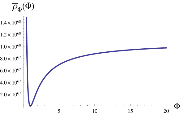
Figure 1 presents the relation . Note that the function has the same shape like the Starobinsky potential. The function has the minimum for
| (37) |
In general, the scalar field is given by (cf. (11))
| (38) |
Because , and taking into account (34) one gets
| (39) |
the algebraic equation determining the function for a given barotropic factor . This provides an implicit dependence . In order to get it more explicit one needs to solve (39) for some interesting values . For example in the case of dust we obtain the third order polynomial equation
where .
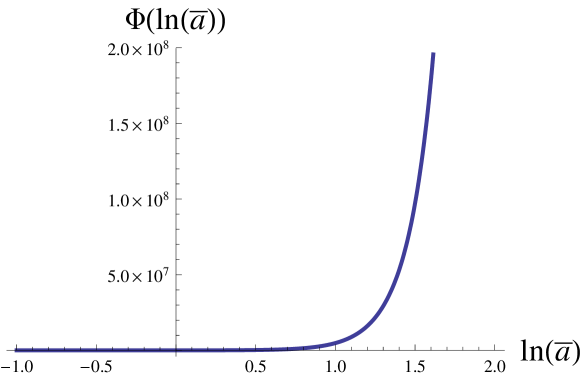
The evolution of , at the beginning of the inflation epoch, is presented in figure 2.
For , the potential can be approximated as . In this case the Friedmann equation can be written as
| (40) |
In the case of , is constant and the Friedmann equation has the following form
| (41) |
In this model the inflation phenomenon appears when the the value of the parameter is close to zero and the matter is negligible with comparison to . In this case the approximate number of e-foldings is given by the following formula
| (42) |
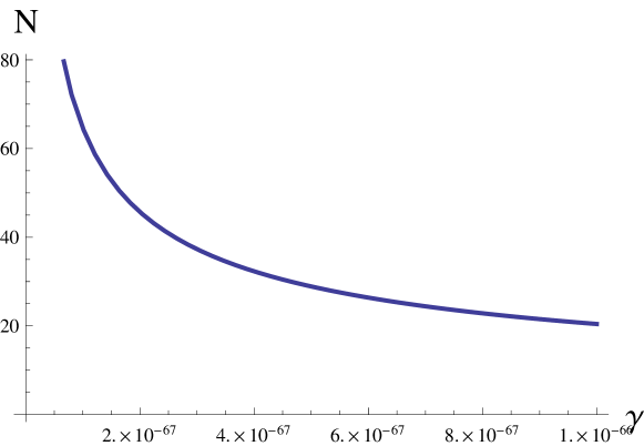
The number of e-folds should be equal in the inflation epoch Cheng:2013iya . In this model we obtain , when and the timescale of the inflation is equal Ade:2014xna . The relation between and the approximate number of e-foldings is presented in figure 3.
The condition for appearing of the inflation requires the value of the parameter to be close to zero, hence the influence of the parameter for the evolution of the universe is negligible.
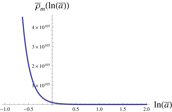
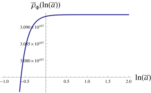
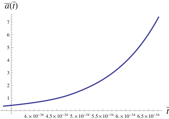
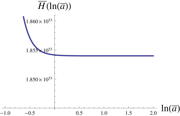
In figure 4 it is demonstrated the typical evolution of at the beginning of the inflation epoch. The typical evolution of , at the beginning of the inflation epoch, is presented in figure 5. Note that, for the late time universe can be approximated as a constant. Figure 6 presents the evolution of the scale factor during the inflation. Figure 7 shows the Hubble function during the inflation epoch.
The conservation equation for can be written as
| (43) |
where is an effective pressure. In this case the equation of state for the dark energy is expressed by the following formula
| (44) |
where the function is given by the expression
| (45) |
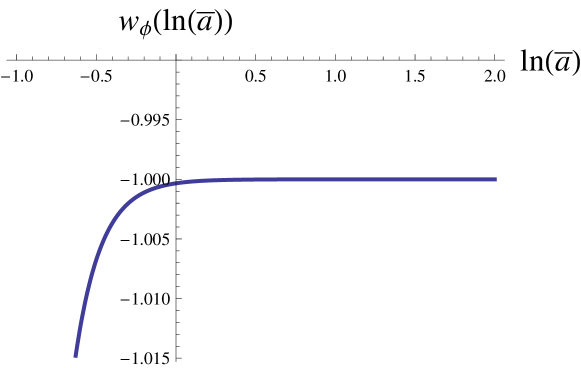
The diagram of coefficient of equation of state , at the beginning the inflation epoch, is presented in figure 8. Note that the function , for the late time, is a constant and equal .
We obtain Brans-Dicke action with the coupling parameter in the Jordan frame. Equations of motion take the form
| (47a) | |||
| (47b) |
In this case the dynamics of the metric is exactly the same as described by the original Palatini equations (2) – (6). On the cosmological ground it means that the scale factor evolves according to the Friedmann equation (13). It has been recently shown that cosmological data favor the value on the level Hrycyna:2014cka .
3 Singularities in cosmological dynamical systems of Newtonian type
There is a class of cosmological models, which dynamics can be reduced to the dynamical system of the Newtonian type. Let consider a homogeneous and isotropic universe with a spatially flat space-time metric of the form
| (48) |
where is the scale factor and is the cosmological time.
Let us consider the energy-momentum tensor for the perfect fluid with energy density and pressure as a source of gravity. In this case the Einstein equations assumes the form of Friedmann equations
| (49) | ||||
| (50) |
where dot denotes differentiation with respect to the cosmic time , is the Hubble function. In our notation we use the natural system of units in which .
We assume that as well as , i.e. that both energy density as well as pressure depends on the cosmic time through the scale factor . The conservation condition reduces to
| (51) |
It would be convenient to rewrite (49) in an equivalent form
| (52) |
where
| (53) |
In (53) plays the model role of effective energy density. For example for the standard cosmological model (12)
| (54) |
where and . Equation (50) is equivalent to
| (55) |
which is called acceleration equation. It is easily to check that
| (56) |
where is given by (53) provided that conservation equation (51) is fulfilled.
Due to equation (56) the evolution of a universe can be interpreted as a motion of a fictitious particle of unit mass in the potential . Here plays the role of a positional variable. Equation of motion (56) assumes the form analogous to the Newtonian equation of motion.
If we know the form of effective energy density then we can construct the form of potential , which determine the whole dynamics in the phase space . In this space the Friedmann equation (52) plays the role of a first integral and determines the phase space curves representing the evolutionary paths of the cosmological models. The diagram of potential contains all information needed to construction of a phase space portrait. In this case the phase space is two-dimensional
| (57) |
In a general case of arbitrary potential, a dynamical system which describes the evolution of a universe takes the form
| (58) | ||||
| (59) |
We shall study the system above using theory of piece-wise smooth dynamical systems. Therefore it is assumed that the potential function, except some isolated (singular) points, belongs to the class .
The lines represent possible evolutions of the universe for different initial conditions. The equations (58) and (59) can be rewritten in dimensionless variables if we replace effective energy density by density parameter
| (60) |
then
| (61) | ||||
| (62) |
where and
| (63) |
Any cosmological model can be identified by its form of the potential function depending on the scale factor . From the Newtonian form of the dynamical system (58)-(59) one can see that all critical points correspond to vanishing of r.h.s of the dynamical system . Therefore all critical points are localized on the -axis, i.e. they represent a static universe.
Because of the Newtonian form of the dynamical system the character of critical points is determined from the characteristic equation of the form
| (64) |
where is determinant of linearization matrix calculated at the critical points, i.e.
| (65) |
From equation (64) and (65) one can conclude that only admissible critical points are the saddle type if or centers type if .
If a shape of the potential function is known (from the knowledge of effective energy density), then it is possible to calculate cosmological functions in exact form
| (66) |
| (67) |
a deceleration parameter, an effective barotropic factor
| (68) |
| (69) |
a parameter of deviation from de Sitter universe FernandezJambrina:2006hj
| (70) |
(note that if , ), effective matter density and pressure
| (71) |
| (72) |
and, finally, a Ricci scalar curvature for the FRW metric (48)
| (73) |
From the formulas above one can observe that the most of them depend on the quantity
| (74) |
This quantity measures elasticity of the potential function, i.e. indicates how the potential changes if the scale factor changes. For example, for the de Sitter universe , the rate of growth of the potential is as the rate of growth of the scale factor is .
In the classification of the cosmological singularities by Fernandez-Jambrina and Lazkoz FernandezJambrina:2006hj the crucial role is played by the parameter . Note that a cosmological sense of this parameter is
| (75) |
In this approach the classification of singularities is based on generalized power and asymptotic expansion of the barotropic index in the equation of state (or equivalently of the deceleration parameter ) in terms of the time coordinate.
4 Degenerated singularities – new type (VI) of singularity – sewn singularities
Recently, due to discovery of an accelerated phase in the expansion of our Universe, many theoretical possibilities for future singularity are seriously considered. If we assume that the Universe expands following the Friedmann equation, then this phase of expansion is driven by dark energy – hypothetical fluid, which violates the strong energy condition. Many of new types of singularities were classified by Nojiri et al. Nojiri:2005sx . Following their classification the type of singularity depends on the singular behavior of the cosmological quantities like: the scale factor , the Hubble parameter , the pressure and the energy density :
-
•
Type 0: ‘Big crunch’. In this type, the scale factor is vanishing and blow up of the Hubble parameter , energy density and pressure .
-
•
Type I: ‘Big rip’. In this type, the scale factor , energy density and pressure are blown up.
-
•
Type II: ‘Sudden’. The scale factor , energy density and Hubble parameter are finite and and the pressure are divergent.
-
•
Type III: ‘Big freeze’. The scale factor is finite and the Hubble parameter , energy density and pressure are blown up Barrow:2004xh or divergent BouhmadiLopez:2006fu .
-
•
Type IV. The scale factor , Hubble parameter , energy density , pressure and are finite but higher derivatives of the scale factor diverge.
-
•
Type V. The scale factor is finite but the energy density and pressure vanish.
Following Królak Krolak:1986tp , big rip and big crunch singularities are strong whereas sudden, big freeze and type IV are weak singularities.
In the model under consideration the potential function or/and its derivative can diverge at isolated points (value of the scale factor). Therefore mentioned before classification has application only for a single component of piece-wise smooth potential. In our model the dynamical system describing evolution of a universe belongs to the class of a piecewise smooth dynamical systems. As a consequence new types of singularities at finite scale factor can appear for which does not exist (is not determined). This implies that the classification of singularities should be extended to the case of non-isolated singularities.
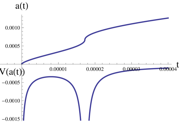
Let us illustrate this idea on the example of freeze singularity in the Starobinsky model with the Palatini formalism (previous section). Such a singularity has a complex character and in analogy to the critical point we called it degenerated. Formally it is composed of two types III singularities: one in the future and another one in the past. If we considered the evolution of the universe before this singularity we detect isolated singularity of type III in the future. Conversely if we consider the evolution after the singularity then going back in time we meet type III singularity in the past. Finally, at the finite scale factor both singularities will meet together. For description of behavior near the singularity one considers relation. This relation has a horizontal inflection point and it is natural to expand this relation in the Taylor series near this point at which is zero. For the freeze singularity, the scale factor remains constant , and blow up and is undefined. It this case, the degenerated singularity of type III is called sewn (non-isolated) singularity. We, therefore, obtain Borowiec:2015qrp
| (76) |
Above formula combine two types of behavior near the freeze singularities in the future
| (77) |
and in the past
| (78) |
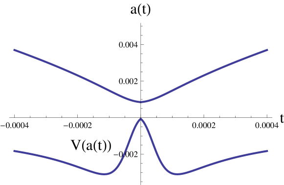
Figure 9 illustrates the behavior of the scale factor in cosmological time in neighborhood of a pole of the potential function. Diagram of is constructed from the dynamics in two disjoint region and . Figure 10 presents the behavior of the scale factor in the cosmological time in a neighborhood of the sudden singularity.
In the model under consideration another type of sewn singularity also appears. It is a composite singularity with two sudden singularities glued at the bounce when . In this singularity the potential itself is a continuous function while its first derivative has a discontinuity. Therefore, the corresponding dynamical system represents a piece-wise smooth dynamical system.
The problem of metric extension beyond the future Cauchy horizon, when the second derivative of the metric is inextendible, was discussed in work of Jan Sbierski Sbierski:2015nta . In the context of FLRW cosmological models, Sbierski’s methodology was considered in Galloway:2016bej .
5 Singularities in the Starobinsky model in the Palatini formalism
In our model, one finds two types of singularities, which are a consequence of the Palatini formalism: the freeze and sudden singularity. The freeze singularity appears when the multiplicative expression , in the Friedmann equation (13), is equal the infinity. So we get a condition for the freeze singularity: which produces a pole in the potential function. It appears that the sudden singularity appears in our model when the multiplicative expression vanishes. This condition is equivalent to the case .
The freeze singularity in our model is a solution of the algebraic equation
| (79) |
or
| (80) |
where .
The solution of the above equation is
| (81) |
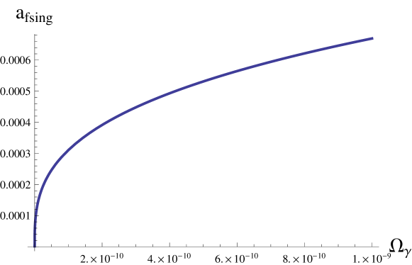
From equation (81), we can find an expression for a value of the scale factor for the freeze singularity
| (82) |
The relation between and positive is presented in Figure 11.
The sudden singularity appears when . This provides the following algebraic equation
| (83) |
The above equation can be rewritten as
| (84) |
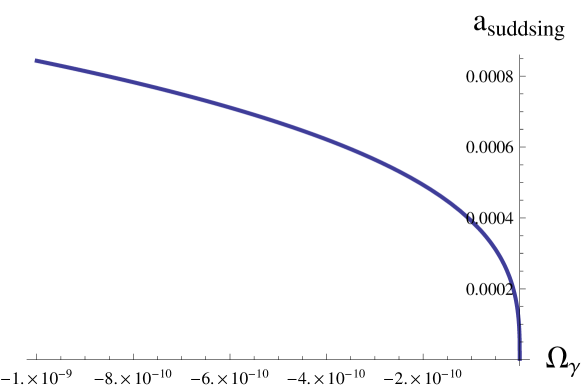
From the equation (84), we have the formula for the scale factor for sudden singularity
| (85) |
which, in fact, becomes a (degenerate) critical point and a bounce at the same time. The relation between and negative is presented in Figure 12.
Let . We can rewrite dynamical system (58)-(59) as
| (86) | ||||
| (87) |
where is a new parametrization of time.
We can treated the dynamical system (86)-(87) as a sewn dynamical system Hrycyna:2008gk ; Ellis:2015bag . In this case, we divide the phase portrait into two parts: the first part is for and the second part is for . Both parts are glued along the singularity.
For , dynamical system (86)-(87) can be rewritten to the corresponding form
| (88) | ||||
| (89) |
where and notes the Heaviside function.
For , in the analogous way, we get the following equations
| (90) | ||||
| (91) |
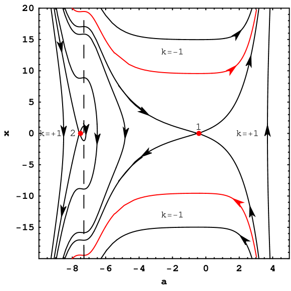
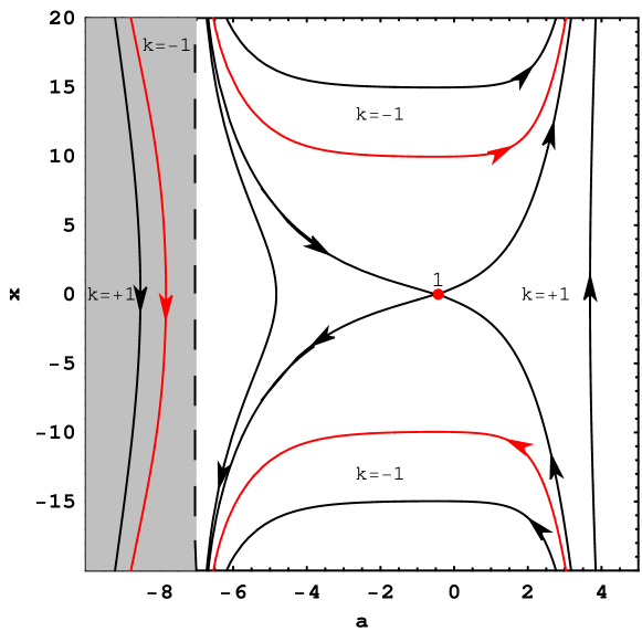
where . The phase portraits, for dynamical system (86)-(87), are presented in Figure 13 and 15. Figure 13 provides the phase portrait for positive while Figure 15 provides the phase portrait for negative .
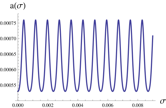
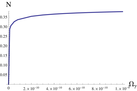
In Figure 13 there are two critical points labelled ‘1’ and ‘2’ at the finite domain. They are both the saddles. These critical points correspond to a maximum of the potential function. The saddle ‘2’ possesses the homoclinic closed orbit starting from it and returning to it. This orbit represents an emerging universe from the static Einstein universe and approaching to it again. During the evolution this universe (orbit) goes two times through the freeze singularity. The region bounded by the homoclinic orbit contains closed orbits representing the oscillating universes. Diagram of the evolution of scale factor for closed orbit is presented by Figure 14. It is also interesting that trajectories in neighborhood of straight vertical line of freeze singularities undergo short time inflation . The characteristic number of e-foldings from to of this inflation period (see formula (3.13) in DeFelice:2010aj ) with respect to is shown in Figure 16. This figure illustrates the number of e-foldings is too small for to obtain the inflation effect.
6 Observations
In this paper we perform statistical analysis using the following astronomical observations: observations of 580 supernovae of type Ia, BAO, measurements of for galaxies, Alcock-Paczyński test, measurements of CMB and lensing by Planck and low by WMAP.
The likelihood function for observations of supernovae of type Ia Suzuki:2011hu is given by the following expression
| (92) |
where , , and is a covariance matrix for observations of supernovae of type Ia. The distance modulus is defined by the formula (where is the apparent magnitude and is the absolute magnitude of observations of supernovae of type Ia) and (where the luminosity distance is ).
BAO observations such as Sloan Digital Sky Survey Release 7 (SDSS DR7) dataset at Percival:2009xn , 6dF Galaxy Redshift Survey measurements at redshift Beutler:2011hx , and WiggleZ measurements at redshift Blake:2012pj have the following likelihood function
| (93) |
where is the sound horizon at the drag epoch Hu:1995en ; Eisenstein:1997ik .
For the Alcock-Paczynski test Alcock:1979mp ; Lopez-Corredoira:2013lca we used the following expression for the likelihood function
| (94) |
where and are observational data Sutter:2012tf ; Blake:2011ep ; Ross:2006me ; Marinoni:2010yoa ; daAngela:2005gk ; Outram:2003ew ; Anderson:2012sa ; Paris:2012iw ; Schneider:2010hm .
The likelihood function for measurements of the Hubble parameter of galaxies from Simon:2004tf ; Stern:2009ep ; Moresco:2012jh is given by the expression
| (95) |
In this paper, we use the likelihood function for observations of CMB Ade:2015rim and lensing by Planck, and low- polarization from the WMAP (WP) in the following form
| (96) |
where is the covariance matrix with the errors, is a vector of the acoustic scale , the shift parameter and where
| (97) | ||||
| (98) |
where is the redshift of the epoch of the recombination Hu:1995en .
The total likelihood function is expressed in the following form
| (99) |
To estimate model parameters, we use our own code CosmoDarkBox. The Metropolis-Hastings algorithm Metropolis:1953am ; Hastings:1970aa is used in this code.
Table 1 completes the values of parameters for the best fit with errors. Figure 17 and Figure 18 show the intersection of a likelihood function with the and confidence level projections on the planes (, ) and (, ).
In this paper, we use Bayesian information criterion (BIC) Schwarz:1978ed ; Kass:1995bf , for comparison our model with the CDM model. The expression for BIC is defined as
| (100) |
where is the value of in the best fit, is the number of model parameters (our model has three parameters, CDM model has two parameters) and is number of data points (), which are used in the estimation.
For our model, the value of BIC is equal 135.668 and for the CDM model BIC. So BIC=BIC-BIC is equal 6.407. The evidence for the model is strong Kass:1995bf if BIC is more than 6. So, in comparison to our model, the evidence in favor of the CDM model is strong, but we cannot absolutely reject our model.
| parameter | best fit | CL | CL |
|---|---|---|---|
| 68.10 | |||
| 0.3011 | |||


7 Conclusions
In this paper, we demonstrated that evolution of the Starobinsky model with a quadratic term gives rise to the description of dynamics in terms of piecewise-smooth dynamical systems (PWS), i.e., systems whose the phase space is partitioned into different regions, each of them associated to a different smooth functional form of the system of a Newtonian type. Different regions of the phase space correspond to different forms of the potential separated by singularities of the type of poles.
Our idea was to obtain the inflation as an endogenous effect of the dynamics in the Palatini formalism. While the effect of inflation appears in the model under consideration the number of sufficient e-folds is not achieved and the additional effect of amplification is required. Note that this type of inflation is a realisation of the idea of singular inflation Barrow:2015ora ; Bamba:2016ngh ; Nojiri:2015wsa ; Odintsov:2015gba . In our model inflation is driven by the freeze degenerated singularity (the extension of type III isolated singularity).
We show that dynamics of the model can be analyzed in terms of two-dimensional dynamical systems of the Newtonian type. In this approach, in the diagram of the potential of a fictitious particle mimicking, the evolution of the universe contain all information which are needed for investigation of singularities in the model. Note that they are not isolated singularities which were classified into five types but rather double singularities glued in one point of the evolution at . Appearance of such types of singularities is typical for piece-wise smooth dynamics describing the model evolution. We called this type of sewn singularities in analogy to sewn dynamical systems Zhusubaliyev:2003bc ; Leine:2004db .
We investigated the model with , where assumes the positive or negative values. While the dynamics of this class of models depend crucially on the sign of the parameter in the early universe for the late time we obtain the behavior consistent with the CDM model.
Note that in the model with positive , the phase space is a sum of two disjoint domains which boundary represents the double freeze singularity (cf. Figure 13). In the first domain the evolution starts from big-bang followed by the deceleration phase then changes to acceleration (early acceleration inflation) after reaching a maximum of the potential function. In the second domain, on the right from the vertical line of the freeze singularity, the universe decelerates and after reaching another maximum starts to accelerate again. This last eternal acceleration correspond to the present day epoch called dark energy domination epoch. Two phases of deceleration and two phases of acceleration are key ingredients of our model. While the first phase models a transition from the matter domination epoch to the inflation the second phase models a transition from the second matter dominated epoch toward the present day acceleration.
As De Felice and Tsujikawa have noted (DeFelice:2010aj, , p. 24) the applications of theories should be focused on construct of viable cosmological models, for which a sequence of radiation, matter and accelerating epochs is realized. All these epochs are also presented in the model under consideration but, for negative (negative squared for the scalar field), some difficulties appear in the interpretation of the phase space domain . The size of this domain will depend on the value of the parameter and this domain vanishes as we are going toward equal zero.
On the other hand it is well know that violation of condition gives rise to the negative values of . We do not assume this condition but we require that to avoid the appearance of ghosts (see section 7.4 in DeFelice:2010aj ). In our case, statistical analysis more favors model with () than with (). In other words, statistical analysis more favors the case without ghosts.
In order to obtain deeper insight into the model we have also performed complementary investigations in the Einstein frame. In this case we obtain that the model is reduced to the FRW cosmological model with the selfinteracting scalar field and the vanishing part of the kinetic energy. Therefore from the Palatini formulation we obtain directly the form of the potential and the (implicit) functional dependence between the scalar field and the scale factor. Moreover, we obtain the parametrization of the decaying cosmological constant.
Due to time dependent cosmological constant the model evolution can be described in terms of an interaction between the matter and the decaying lambda terms. We study how the energy is transferred between sectors and how the standard scaling relation for matter is modified.
We pointed out that the consideration of the Starobinsky model in the Einstein frame gives rise to new interesting properties from the cosmological point of view similarly as the original (metric) Starobinsky model is very important for the explanation of the inflation. The model under the consideration gives rise analogously to the running cosmological term. This fact seems to be interesting in the context of an explanation of the cosmological constant problem.
Detailed conclusions coming from our analysis are the following:
-
•
We show that the interaction between two sectors: the matter and the decaying vacuum, appears naturally in the Einstein frame. For the model formulated in the Jordan frame this interaction is absent.
-
•
The inflation appears in our model formulated in the Einstein frame, when the parameter is close to zero and the density of matter is negligible in comparison to .
-
•
In our model in the Einstein frame, the potential has the same shape like the Starobinsky potential and has the minimum for .
-
•
While the freeze double singularities appear in our model in the Jordan frame there is no such singularities in the dynamics of the model in the Einstein frame.
-
•
If is small, then for negative and for positive . These values defines the natural scale at which singularities appear in the model under consideration with the negative or positive value of parameter. It seems to be natural to identify this scale with a cut off at which the model can be treated as some kind of effective theory.
-
•
In both cases of negative and positive one deals with a finite scale factor singularity. For negative it is a double sudden singularity which meets the future singularity of contracting model before the bounce with the initial singularity in the expanding model. The sewn evolutionary scenarios reveal the presence of bounce during the cosmic evolution.
-
•
In the context of the Starobinsky model in the Palatini formalism we found a new type of double singularity beyond the well-known classification of isolated singularities.
-
•
The phase portrait for the model with a positive value of is equivalent to the phase portrait of the CDM model (following the dynamical system theory Perko:2001de equivalence assumes the form of topological equivalence establish by homeomorphism). There is only a quantitative difference related with the presence of the non-isolated freeze singularity. The scale of appearance of this type singularity can be also estimated and in terms of redshift: .
-
•
We estimated the model parameters using astronomical data and conclude that positive is favored by the best fit value; still the model without term is statistically admitted.
In our model, the best fit value of is equal and positive parameter belongs to the interval at 2- level. This mean that the positive value of is more favored by astronomical data than the negative value of . The difference between values of BIC for our model and the CDM model is equal 6.407. So, in comparison to our model, the evidence in favor of the CDM model is strong. But one cannot absolutely reject the model.
Note added in proof. After completing the paper we found a paper by Faraoni and Cardini where freeze singularities have been analyzed in a different context, both from point particle and cosmological perspectives Faraoni:2016lhd .
Acknowledgements.
AB and MS would like to thank Salvatore Capozziello for encouraging us to consider this model in different frames. The work has been supported by the Polish National Science Centre (NCN), project DEC-2013/09/B/ ST2/03455.References
- (1) A. De Felice and S. Tsujikawa, f(R) theories, Living Rev. Rel. 13 (2010) 3, [arXiv:1002.4928].
- (2) A. A. Starobinsky, A New Type of Isotropic Cosmological Models Without Singularity, Phys. Lett. B91 (1980) 99–102.
- (3) A. H. Guth, The Inflationary Universe: A Possible Solution to the Horizon and Flatness Problems, Phys. Rev. D23 (1981) 347–356.
- (4) A. D. Linde, Eternally Existing Selfreproducing Chaotic Inflationary Universe, Phys. Lett. B175 (1986) 395–400.
- (5) S. Nojiri and S. D. Odintsov, Introduction to modified gravity and gravitational alternative for dark energy, Int. J. Geom. Meth. Mod. Phys. 4 (2007) 115, [hep-th/0601213].
- (6) T. P. Sotiriou and V. Faraoni, f(R) Theories of Gravity, Rev. Mod. Phys. 82 (2010) 451–497, [arXiv:0805.1726].
- (7) V. F. Mukhanov and G. V. Chibisov, Quantum Fluctuations and a Nonsingular Universe, JETP Lett. 33 (1981) 532–535. [Pisma Zh. Eksp. Teor. Fiz.33,549(1981)].
- (8) A. A. Starobinsky, The Perturbation Spectrum Evolving from a Nonsingular Initially De-Sitter Cosmology and the Microwave Background Anisotropy, Sov. Astron. Lett. 9 (1983) 302.
- (9) Planck Collaboration, P. A. R. Ade et al., Planck 2015 results. XIV. Dark energy and modified gravity, Astron. Astrophys. 594 (2016) A14, [arXiv:1502.01590].
- (10) C. Cheng, Q.-G. Huang, and Y.-Z. Ma, Constraints on single-field inflation with WMAP, SPT and ACT data — a last-minute stand before Planck, JCAP 1307 (2013) 018, [arXiv:1303.4497].
- (11) Q.-G. Huang, A polynomial f(R) inflation model, JCAP 1402 (2014) 035, [arXiv:1309.3514].
- (12) L. A. Kofman, A. D. Linde, and A. A. Starobinsky, Inflationary Universe Generated by the Combined Action of a Scalar Field and Gravitational Vacuum Polarization, Phys. Lett. B157 (1985) 361–367.
- (13) S. V. Ketov and A. A. Starobinsky, Embedding ()-Inflation into Supergravity, Phys. Rev. D83 (2011) 063512, [arXiv:1011.0240].
- (14) S. A. Appleby, R. A. Battye, and A. A. Starobinsky, Curing singularities in cosmological evolution of F(R) gravity, JCAP 1006 (2010) 005, [arXiv:0909.1737].
- (15) S. Capozziello, M. De Laurentis, S. Nojiri, and S. D. Odintsov, Classifying and avoiding singularities in the alternative gravity dark energy models, Phys. Rev. D79 (2009) 124007, [arXiv:0903.2753].
- (16) A. Alho, S. Carloni, and C. Uggla, On dynamical systems approaches and methods in cosmology, JCAP 1608 (2016), no. 08 064, [arXiv:1607.05715].
- (17) S. Capozziello, M. F. De Laurentis, L. Fatibene, M. Ferraris, and S. Garruto, Extended Cosmologies, SIGMA 12 (2016) 006, [arXiv:1509.08008].
- (18) S. Capozziello, P. Martin-Moruno, and C. Rubano, Physical non-equivalence of the Jordan and Einstein frames, Phys. Lett. B689 (2010) 117–121, [arXiv:1003.5394].
- (19) S. M. Carroll, A. De Felice, V. Duvvuri, D. A. Easson, M. Trodden, and M. S. Turner, The Cosmology of generalized modified gravity models, Phys. Rev. D71 (2005) 063513, [astro-ph/0410031].
- (20) A. Borowiec, M. Kamionka, A. Kurek, and M. Szydlowski, Cosmic acceleration from modified gravity with Palatini formalism, JCAP 1202 (2012) 027, [arXiv:1109.3420].
- (21) T. Koivisto, Covariant conservation of energy momentum in modified gravities, Class. Quant. Grav. 23 (2006) 4289–4296, [gr-qc/0505128].
- (22) L. Fernandez-Jambrina and R. Lazkoz, Classification of cosmological milestones, Phys. Rev. D74 (2006) 064030, [gr-qc/0607073].
- (23) S. Bahamonde, S. D. Odintsov, V. K. Oikonomou, and P. V. Tretyakov, Deceleration versus acceleration universe in different frames of gravity, Phys. Lett. B766 (2017) 225–230, [arXiv:1701.02381].
- (24) M. P. Dabrowski, J. Garecki, and D. B. Blaschke, Conformal transformations and conformal invariance in gravitation, Annalen Phys. 18 (2009) 13–32, [arXiv:0806.2683].
- (25) BICEP2 Collaboration, P. A. R. Ade et al., Detection of -Mode Polarization at Degree Angular Scales by BICEP2, Phys. Rev. Lett. 112 (2014), no. 24 241101, [arXiv:1403.3985].
- (26) O. Hrycyna, M. Szydlowski, and M. Kamionka, Dynamics and cosmological constraints on Brans-Dicke cosmology, Phys. Rev. D90 (2014), no. 12 124040, [arXiv:1404.7112].
- (27) S. Nojiri, S. D. Odintsov, and S. Tsujikawa, Properties of singularities in (phantom) dark energy universe, Phys. Rev. D71 (2005) 063004, [hep-th/0501025].
- (28) J. D. Barrow, Sudden future singularities, Class. Quant. Grav. 21 (2004) L79–L82, [gr-qc/0403084].
- (29) M. Bouhmadi-Lopez, P. F. Gonzalez-Diaz, and P. Martin-Moruno, Worse than a big rip?, Phys. Lett. B659 (2008) 1–5, [gr-qc/0612135].
- (30) A. Krolak, Towards the proof of the cosmic censorship hypothesis, Class. Quant. Grav. 3 (1986) 267–280.
- (31) A. Borowiec, A. Stachowski, M. Szydlowski, and A. Wojnar, Inflationary cosmology with Chaplygin gas in Palatini formalism, JCAP 1601 (2016), no. 01 040, [arXiv:1512.01199].
- (32) J. Sbierski, The -inextendibility of the Schwarzschild spacetime and the spacelike diameter in Lorentzian geometry, arXiv:1507.00601.
- (33) G. Galloway and E. Ling, Some remarks on the -(in)extendibility of spacetimes, arXiv:1610.03008.
- (34) O. Hrycyna and M. Szydlowski, Non-minimally coupled scalar field cosmology on the phase plane, JCAP 0904 (2009) 026, [arXiv:0812.5096].
- (35) G. F. R. Ellis, E. Platts, D. Sloan, and A. Weltman, Current observations with a decaying cosmological constant allow for chaotic cyclic cosmology, JCAP 1604 (2016), no. 04 026, [arXiv:1511.03076].
- (36) N. N. Bautin and I. A. Leontovich, eds., Methods and Techniques for Qualitative Analysis of Dynamical Systems on the Plane. Nauka, Moscow, 1976. [In Russian].
- (37) N. Suzuki et al., The Hubble Space Telescope Cluster Supernova Survey: V. Improving the Dark Energy Constraints Above and Building an Early-Type-Hosted Supernova Sample, Astrophys. J. 746 (2012) 85, [arXiv:1105.3470].
- (38) SDSS Collaboration, W. J. Percival et al., Baryon Acoustic Oscillations in the Sloan Digital Sky Survey Data Release 7 Galaxy Sample, Mon. Not. Roy. Astron. Soc. 401 (2010) 2148–2168, [arXiv:0907.1660].
- (39) F. Beutler, C. Blake, M. Colless, D. H. Jones, L. Staveley-Smith, L. Campbell, Q. Parker, W. Saunders, and F. Watson, The 6dF Galaxy Survey: Baryon Acoustic Oscillations and the Local Hubble Constant, Mon. Not. Roy. Astron. Soc. 416 (2011) 3017–3032, [arXiv:1106.3366].
- (40) C. Blake et al., The WiggleZ Dark Energy Survey: Joint measurements of the expansion and growth history at , Mon. Not. Roy. Astron. Soc. 425 (2012) 405–414, [arXiv:1204.3674].
- (41) W. Hu and N. Sugiyama, Small scale cosmological perturbations: An analytic approach, Astrophys. J. 471 (1996) 542–570, [astro-ph/9510117].
- (42) D. J. Eisenstein and W. Hu, Baryonic features in the matter transfer function, Astrophys. J. 496 (1998) 605, [astro-ph/9709112].
- (43) C. Alcock and B. Paczynski, An evolution free test for non-zero cosmological constant, Nature 281 (1979) 358–359.
- (44) M. Lopez-Corredoira, Alcock-Paczynski cosmological test, Astrophys. J. 781 (2014), no. 2 96, [arXiv:1312.0003].
- (45) P. M. Sutter, G. Lavaux, B. D. Wandelt, and D. H. Weinberg, A first application of the Alcock-Paczynski test to stacked cosmic voids, Astrophys. J. 761 (2012) 187, [arXiv:1208.1058].
- (46) C. Blake et al., The WiggleZ Dark Energy Survey: measuring the cosmic expansion history using the Alcock-Paczynski test and distant supernovae, Mon. Not. Roy. Astron. Soc. 418 (2011) 1725–1735, [arXiv:1108.2637].
- (47) N. P. Ross et al., The 2dF-SDSS LRG and QSO Survey: The 2-Point Correlation Function and Redshift-Space Distortions, Mon. Not. Roy. Astron. Soc. 381 (2007) 573–588, [astro-ph/0612400].
- (48) C. Marinoni and A. Buzzi, A geometric measure of dark energy with pairs of galaxies, Nature 468 (2010), no. 7323 539–541.
- (49) J. da Angela, P. J. Outram, and T. Shanks, Constraining beta(z) and Omega 0(m) from redshift-space distortions in z 3 galaxy surveys, Mon. Not. Roy. Astron. Soc. 361 (2005) 879–886, [astro-ph/0505469].
- (50) P. J. Outram, T. Shanks, B. J. Boyle, S. M. Croom, F. Hoyle, N. S. Loaring, L. Miller, and R. J. Smith, The 2df qso redshift survey. 13. A measurement of lambda from the qso power spectrum, Mon. Not. Roy. Astron. Soc. 348 (2004) 745, [astro-ph/0310873].
- (51) L. Anderson et al., The clustering of galaxies in the SDSS-III Baryon Oscillation Spectroscopic Survey: Baryon Acoustic Oscillations in the Data Release 9 Spectroscopic Galaxy Sample, Mon. Not. Roy. Astron. Soc. 427 (2013), no. 4 3435–3467, [arXiv:1203.6594].
- (52) I. Paris et al., The Sloan Digital Sky Survey quasar catalog: ninth data release, Astron. Astrophys. 548 (2012) A66, [arXiv:1210.5166].
- (53) SDSS Collaboration, D. P. Schneider et al., The Sloan Digital Sky Survey Quasar Catalog V. Seventh Data Release, Astron. J. 139 (2010) 2360–2373, [arXiv:1004.1167].
- (54) J. Simon, L. Verde, and R. Jimenez, Constraints on the redshift dependence of the dark energy potential, Phys. Rev. D71 (2005) 123001, [astro-ph/0412269].
- (55) D. Stern, R. Jimenez, L. Verde, M. Kamionkowski, and S. A. Stanford, Cosmic Chronometers: Constraining the Equation of State of Dark Energy. I: H(z) Measurements, JCAP 1002 (2010) 008, [arXiv:0907.3149].
- (56) M. Moresco et al., Improved constraints on the expansion rate of the Universe up to z 1.1 from the spectroscopic evolution of cosmic chronometers, JCAP 1208 (2012) 006, [arXiv:1201.3609].
- (57) N. Metropolis, A. W. Rosenbluth, M. N. Rosenbluth, A. H. Teller, and E. Teller, Equation of state calculations by fast computing machines, J. Chem. Phys. 21 (1953) 1087–1092.
- (58) W. K. Hastings, Monte Carlo Sampling Methods Using Markov Chains and Their Applications, Biometrika 57 (1970) 97–109.
- (59) G. Schwarz, Estimating the dimension of a model, Ann. Statist. 6 (1978), no. 2 461–464.
- (60) R. E. Kass and A. E. Raftery, Bayes factors, J. Amer. Stat. Assoc. 90 (1995) 773–795.
- (61) J. D. Barrow and A. A. H. Graham, Singular Inflation, Phys. Rev. D91 (2015), no. 8 083513, [arXiv:1501.04090].
- (62) K. Bamba, Inflationary universe in fluid description, 2016. arXiv:1601.04773.
- (63) S. Nojiri, S. D. Odintsov, and V. K. Oikonomou, Singular inflation from generalized equation of state fluids, Phys. Lett. B747 (2015) 310–320, [arXiv:1506.03307].
- (64) S. D. Odintsov and V. K. Oikonomou, Singular Inflationary Universe from Gravity, Phys. Rev. D92 (2015), no. 12 124024, [arXiv:1510.04333].
- (65) Z. T. Zhusubaliyev and E. Mosekilde, Bifurcations and Chaos in Piecewise-Smooth Dynamical Systems. World Scientific, Singapore, 2003.
- (66) R. Leine and H. Nijmeijer, Dynamics and Bifurcations of Non-Smooth Mechanical Systems. Springer, Berlin, 2004.
- (67) L. Perko, Differential Equations and Dynamical Systems, vol. 7 of Texts in Applied Mathematics. Springer, New York, third ed., 2001.
- (68) V. Faraoni and A. M. Cardini, Analogues of glacial valley profiles in particle mechanics and in cosmology, arXiv:1608.02542.