A PSF-based approach to Kepler/K2 data. II. Exoplanet candidates in Praesepe (M 44)

Abstract

In this work we keep pushing K2 data to a high photometric precision, close to that of the Kepler main mission, using a PSF-based, neighbour-subtraction technique, which also overcome the dilution effects in crowded environments. We analyse the open cluster M 44 (NGC 2632), observed during the K2 Campaign 5, and extract light curves of stars imaged on module 14, where most of the cluster lies. We present two candidate exoplanets hosted by cluster members and five by field stars. As a by-product of our investigation, we find 1680 eclipsing binaries and variable stars, 1071 of which are new discoveries. Among them, we report the presence of a heartbeat binary star. Together with this work, we release to the community a catalogue with the variable stars and the candidate exoplanets found, as well as all our raw and detrended light curves.

1 Introduction

K2 mission (Howell et al., 2014) has further boosted the “gold rush” of the exoplanet hunting. While many exoplanets have been found around field stars, only a few of them have been detected orbiting around stellar-cluster members. The discovery and characterisation of these cluster-hosted objects is very important to add a new piece to their puzzling formation and evolutionary scenarios.

K2, as well as Kepler (Borucki et al., 2010), gives us the opportunity to search for exoplanet candidates for radial-velocity follow-ups in different open (with ages spanning from about the 100 Myrs of Pleiades to the $\sim$8.3 Gyr of NGC 6791) and globular (M 4 and M 80) clusters.

In our first work, (Libralato et al., 2016, hereafter Paper I), we showed that by using a high-angular-resolution catalogue and point-spread functions (PSFs) we are able to pinpoint each star in the adopted input catalogue into each K2 exposure and to measure its flux after all detectable close-by neighbours are subtracted from the image. This PSF-based technique allows us to (i) increase the number of analysable objects in the field, (ii) estimate an unbiased flux for a given source, (iii) extract the light curve (LC) of a star in a crowded environment and (iv) improve the photometric precision reachable for faint stars ($K_{\rm P}\gtrsim 15.5)$.

In this work, we continue our effort on stellar clusters, focusing on the open cluster (OC) Praesepe (NGC 2632, hereafter simply M 44) that was observed between 2015 April 27 and 2015 July 10 during the K2 Campaign 5 (hereafter, C5). We applied our PSF-based approach described in Paper I to extract the LCs of the stars imaged on the isolated target-pixel files (TPFs) of module 14, where most of the cluster stars are observed. Although M 44 is sparser than the field studied in Paper I and not in a super-stamp, our technique is perfectly suitable to also analyse this cluster.

M 44 is one of the few stellar clusters in which exoplanets have been detected. Using the radial-velocity (RV) technique, two hot Jupiters were found by Quinn et al. (2012), each of them around a M 44 main-sequence (MS) star. Later, in a long-term RV monitoring of M 44 members, Malavolta et al. (2016) found an additional, massive Jupiter in a very-eccentric orbit hosted by one of the two aforementioned MS stars, discovering de facto the first multi-planet system in an OC. From the photometric point of view, before K2 started operations, during the Kilodegree Extremely Little Telescope (KELT) survey Pepper et al. (2008) revealed two transiting exoplanet candidates in M 44 field, but their proper motions exclude their membership to the cluster (see Sect. 5.3). Driven by these promising results, we explored the K2/C5 data to search for additional (transiting) exoplanets hosted by M 44 members, taking advantage of the high-precision photometry and the almost-uninterrupted time series released by K2.

2 Data reduction

2.1 Asiago Schmidt telescope

As in Paper I, we used a high-angular-resolution input list to perform our neighbour-subtraction technique. We observed M 44 in seven nights (between 2015 March 27 and April 22) using the Asiago 67/92 cm Schmidt telescope on Mount Ekar. A SBIG STL-11000M camera, equipped with a Kodak KAI-11000M detector (4050$\times$2672 pixel² with a pixel scale of 0.8625 arcsec pixel^-1), is placed at the focus of the telescope and covers a field of view (FoV) of about 58$\times$38 arcmin².

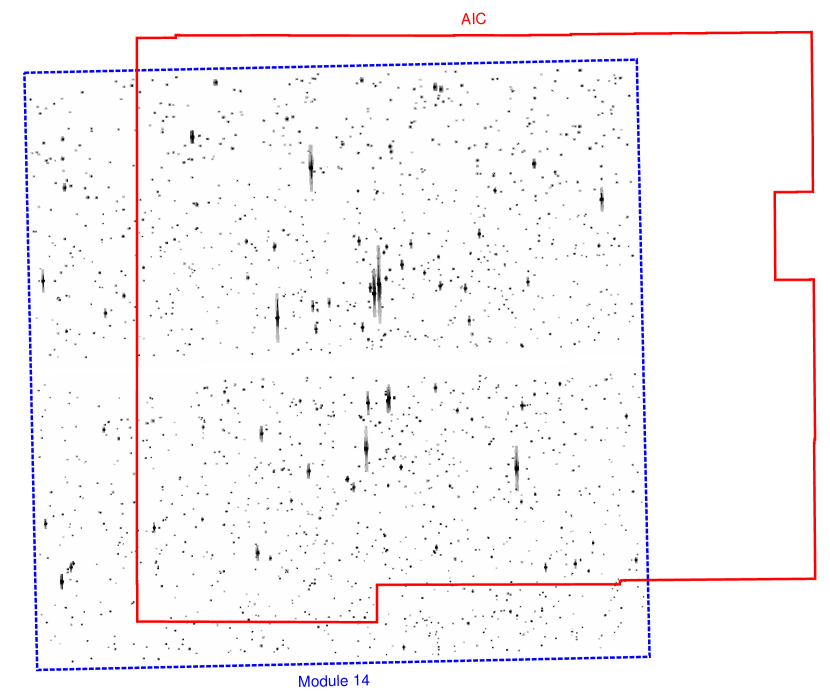
The FoV covered by our observations is of about 2.7$\times$2.3 deg² on the sky, and was obtained by adopting a specific, dithered observing strategy in order to cover the most of the cluster. However, this observing campaign was performed prior to the K2/C5 data release, therefore the field overlap between our Asiago Schmidt and the K2/C5 data is not perfect (see Fig. 1). In total, we collected 120-s exposures in white light (unfiltered solution, hereafter $N$ filter; 123 images), $B$ (48), $R$ (81) and $I$ (81) filters. For each image, we created a set of 9$\times$5 spatially-varying, empirical PSFs and used them to measure positions and fluxes for all the detectable objects in the field. The dedicated software was developed starting from the work of Anderson et al. (2006) with the wide-field imager at the 2.2 m MPI/ESO telescope. Stellar positions were also corrected for geometric distortion.

The input catalogue was built as described in detail by Nardiello et al. (2015). Briefly, we started by making the $N$-filter input list. We transformed (by mean of six-parameter linear transformations) all $N$-filter stellar catalogues into the reference frame system of the best (minimum of the product between airmass and seeing) image. We then created a stacked image which high signal-to-noise ratio (SNR) allowed us to better analyse faint sources. As for the single exposures, we generated an array of spatially-varying, empirical PSFs and measured all detectable objects over the entire FoV covered by the stacked image. Spurious detections and PSF artefacts were removed from the input list by using a parameter called quality of the PSF fit (QFIT, Anderson et al., 2008), the method described in Libralato et al. (2014) and by visually inspecting the stacked image.

The same procedure was performed to obtain the stellar list for the other filters. The $B$, $R$ and $I$ magnitudes were calibrated by using the catalogue of An et al. (2007). We selected a sample of bright, unsaturated stars in our catalogue in common with that of An et al., and performed a least-square fit to find the coefficients of the calibration equations. We found that a linear relation was enough to register our photometry.

Finally we cross-identified all stars among the different catalogues and create a multi-filter input list for M 44. The catalogue, that contains about 24 000 stars measured in $N$ filter, was also linked to the Two Micron All-Sky Survey (2MASS, Skrutskie et al., 2006) catalogue to have for each star a $J_{\rm 2MASS}$-, $H_{\rm 2MASS}$-, $K_{\rm 2MASS}$-magnitude entry (when available), and to the PPMXL catalogue (Roeser, Demleitner, & Schilbach, 2010) for the ($\mu_{\alpha}\cos\delta$,$\mu_{\delta}$) proper motions. Hereafter we refer to this catalogue as the Asiago Input Catalogue (AIC).

Figure 1: K2 module-14 FoV covered during C5. The image is a mosaic of four stacked images, one for each channel. Each stacked image was obtained by combining all 3620 usable exposures that we used in the LC extraction. The blue, dashed rectangle represents K2 module 14, while the red, solid rectangle shows the Asiago-Input-Catalog (AIC) coverage. The image is in logarithmic grey scale; North is up and East to the left.

2.2 K2

The K2/C5 data set was reduced following the prescriptions given in Paper I. We analysed the entire module 14 in which M 44 is mainly imaged, namely channels 45, 46, 47 and 48. For each channel, we reconstructed a full-frame exposure for each of the 3620 usable (no-evident trailing effects) K2/C5 cadence number of the TPFs. The average Kepler Barycentric Julian Day (KBJD) of all the TPFs with the same cadence number was then set as KBJD of the reconstructed image. As in Paper I, the column FLUX was used to assign the pixel values.

To model the undersampled PSF of each Kepler channel, we used again the effective-PSF (ePSF) formalism of Anderson & King (2000). The ePSFs were mainly modelled following the prescriptions given in Paper I. Here we describe only the differences between the two works.

First, we used the AIC, transformed into the reference frame system of each image, to pinpoint the position of the bright, unsaturated stars selected to model the ePSF. The high angular resolution and the astrometric accuracy of the AIC allowed us to better place the ePSF samplings and overcome the most of the pixel-phase errors. Three (out of four) module-14 channels are not completely covered by the AIC (Fig. 1). However, since our aim was to obtain a reliable, average ePSF model for each channel, this partial coverage was a good compromise to deal with.

Second, we introduced a neighbour-subtraction stage during the (iterative) ePSF-modelling process. Before collecting the ePSF samplings from a given star and model the ePSF, we subtracted (by using the current ePSF model) all its close-by neighbours contained in the AIC in order to decrease the light-contamination effects that would result in a shallower ePSF. A more detailed description of the new method will be published in a subsequent paper of this series focused on the globular cluster M 4 observed during K2 Campaign 2 (Libralato et al., in preparation), in which the improvement using this approach is more evident due to the higher level of crowding with respect to M 44.

Once we converged to an average ePSF model for each channel, we perturbed it for each image to take into account the temporal variation. We performed a 2$\times$2 perturbation that also partially solved for the ePSF spatial variations across the channel FoV. The 2$\times$2 array was chosen as a compromise between modelling the spatial variations of the ePSF and having enough stars to model the ePSF itself in each cell. We also introduced a neighbour-subtraction phase at the ePSF-perturbation stage, using the AIC to find the location of the close-by neighbours to subtract, before tabulating the normalised ePSF residuals (see Paper I, ). For the regions not covered by the AIC we just collected the ePSF residuals subtracting only the most obvious neighbour stars clearly visible in the reconstructed K2 exposures.

It is worth mentioning that, as stated in Paper I, our ePSFs are still not perfect and a non-negligible room for improvements is expected when the pixel-response-function calibration data will be publicly available.

Finally, we measured positions and fluxes of all sources in each K2 reconstructed full-frame exposure with a least-square fit of the ePSF. We then made a common reference frame system (master frame) for each channel by cross-identifying all bright, unsaturated stars from each K2 image. Position and flux of a given star in the master frame were iteratively computed as the clipped average of the positions and fluxes of that star as measured in each K2 exposure and transformed with six-parameter linear transformations and zero-point registration into the master-frame reference system.

3 K2 photometry

We extracted the LCs for most of the objects imaged on module-14 TPFs during K2/C5. Hereafter, we discuss the key ingredients of our method.

3.1 Modified AIC

As shown in Fig. 1, the AIC does not completely cover the entire module-14 FoV, leaving part of channels 45, 46 and 48 partially unexplored. For this reason, we chose to add the most of the missing stars to the AIC using the K2 images themselves, extracting position and flux of these objects as described in Sect. 2.2. Different factors (e.g., photometric zero-points and geometric distortion) may vary across such a large FoV, therefore we performed the procedure described below independently for each channel.

First, we transformed the position of each missing star from a given K2 exposure (reconstructed using all TPFs with cadence number 108564) into that of the AIC by using six-parameter linear transformations and added them to the input catalogue. The positions of the added stars are less precise than those of the stars contained in the original AIC. Furthermore, for these added stars we do not have any control about the light-dilution effects. However, in this way we were able to add, on average, about 130 stars to each channel input list.

Then, we registered the AIC $N$-filter magnitudes into the $K_{\rm P}$-magnitude system of the previously-built K2 master frame. In first approximation, the Asiago Schmidt $N$ filter is rather similar to the Kepler total transmission curve, and in Paper I we used a simple zero-point to transform the AIC white-light magnitudes into $K_{\rm P}$ magnitudes. However, M 44 stars are spread over a wide range of colours in the colour-magnitude diagram (CMD), i.e., $\Delta(B-I)\sim 6$ magnitudes from the upper to the lower MS, and we found that such zero-point was not the same for all colours. Therefore, we performed a photometric calibration by using the ($B-I$) colour to transform the $N$-filter measurements into $K_{\rm P}$ magnitudes. We applied a least-square fit to find the coefficients of the polynomial to use for such photometric calibration. If either $B$ or $I$ magnitudes were not available for a given star, we adopted the average zero-point between $N$-filter and $K_{\rm P}$ magnitudes. For the added stars, which magnitudes are already in the $K_{\rm P}$ system, we used a simple zero-point between the K2 selected exposure and the K2 master frame to adjust the magnitudes.

At the end of our integration process, we have four modified AICs (mAICs), one for each channel, that differ each other for the number of added stars and for the slightly different calibration equation. Such mAICs were finally used as input lists during the LC-extraction phase.

3.2 Light-curve extraction and systematic correction

For each channel, we extracted the LCs for all objects in the corresponding mAIC as described in Nardiello et al. (2015, 2016) and Paper I. Briefly, for each target star in our input list we used six-parameter, global linear transformations to convert its mAIC position into that of each individual K2 exposure. Only bright, well-measured unsaturated stars were used to compute the coefficients of these transformations. We then measured its flux both in the original and in the neighbour-subtracted images. In the latter case, we subtracted from the image all close-by stars which light contamination would affect the LC of our target. M 44 field is rather sparse, however, in some cases, there are close-by stars for which the light-dilution effects can be important during the LC analysis. For each star we performed 1-, 1.5-, 2- and 2.5-pixel aperture and PSF-fitting photometry. Hereafter, we will consider only the neighbour-subtracted LCs.

The LCs were corrected for the different systematic effects that usually harm K2 data. At variance with K2 Campaign 0, the spacecraft drift was smaller. By simply applying the position-dependent correction of Paper I, we found that the result was not very good, in particular since a few day before the mid-Campaign Argabrightening event when the stars on the CCDs changed drift pattern because of the change of the relative positioning of the spacecraft with respect to the Sun. Furthermore, several stars showed long-term effects not ascribable to intrinsic variability. Therefore, we improved our LC detrend with respect to our first work and added a new, preliminary correction. We refer to our companion paper on the same K2/C5 data (Nardiello et al., MNRAS submitted) focused on the OC M 67 for a detailed description of this systematic-correction stage. In a nutshell, the correction can be summarised as follows.

Figure 2: Photometric precision, represented by the 6.5-h rms, achieved with 1-pixel-aperture (purple points), 1.5-pixel-aperture (black points), 2-pixel-aperture (green points), 2.5-pixel-aperture (red points) and PSF (azure points) photometry on the neighbour-subtracted LCs. We plot the results for each of the four channels of K2 module 14 separately for clarity. The grey, solid horizontal lines are set at 100, 40 and 20 ppm. The saturation threshold ($K_{\rm P}\sim 11.7$) is shown with a grey, solid vertical line.

We first removed the most of the systematic trends that are in common among the different LCs in a given K2 channel. To this task we used the cotrending basis vectors (CBVs) released with each K2 Campaign data set from the third onward, in a similar way as done by the official Kepler pipeline. For each normalised-flux raw LC we modelled the systematic trends using a linear combination of the CBVs. The coefficients of such combination were computed adopting a Levenberg-Marquardt minimisation method (Moré, Garbow, & Hillstrom, 1980). For variable stars we noticed that sometimes the cotrend algorithm tries to include the stellar variability as well in the CBV linear combination, causing a worsening of the LC. For this reason, for each star we checked if the LC scatter (defined as the point-to-point, or p2p, rms of Paper I, ) improved after this cotrend stage. If not, we used as coefficients of the CBV combination the average coefficients computed for all stars across the channel. This way we found an improvement of the LC scatter, even if sometimes it left some long-term systematics.

The cotrend correction also partially compensated for the drift-induced trends. However, the correction was based on the common behaviour of the stars on the CCD, therefore, in order to fine tune it, we applied to each LC our iterative, position-based detrend as done in Paper I. Briefly, we first normalised the raw LC by its median flux and created a LC model. At odds of Paper I, the LC model was not obtained with a running-median filter, but with a linear interpolation. We segmented the LC in different bins and, in each bin, we computed the 3.5$\sigma$-clipped average flux of the points. The boundaries of each bin were defined by two consecutive thruster-jet firings, identified thanks to the “jumps” in the $x$/$y$ raw positions during time. The LC model was generated by linearly interpolating the LC among these bin average values. Finally, we removed the correlation between ($x$,$y$) raw positions and model-subtracted-LC fluxes with a look-up table of correction applied with a simple bi-linear interpolation. By working with the model-subtracted LC, we avoided to wrongly correct also the intrinsic variability of the star.

This correction, in particular the cotrend part, is still in a preliminary phase. Indeed, we used all 16 CBVs to perform the correction. In most cases, the correction works very well. However, a few stars still show residual long-term systematic effects that could hamper, even if only partially, a variability study. The best solution should be to check all the possible combinations of CBVs and find which combination leads to the best photometric precision and preserves the intrinsic stellar signal. Since such long terms do not affect the search for eclipsing or transiting objects on these processed LCs, we postpone the refinement of this cotrend correction to future works of the series.

3.3 Photometric precision

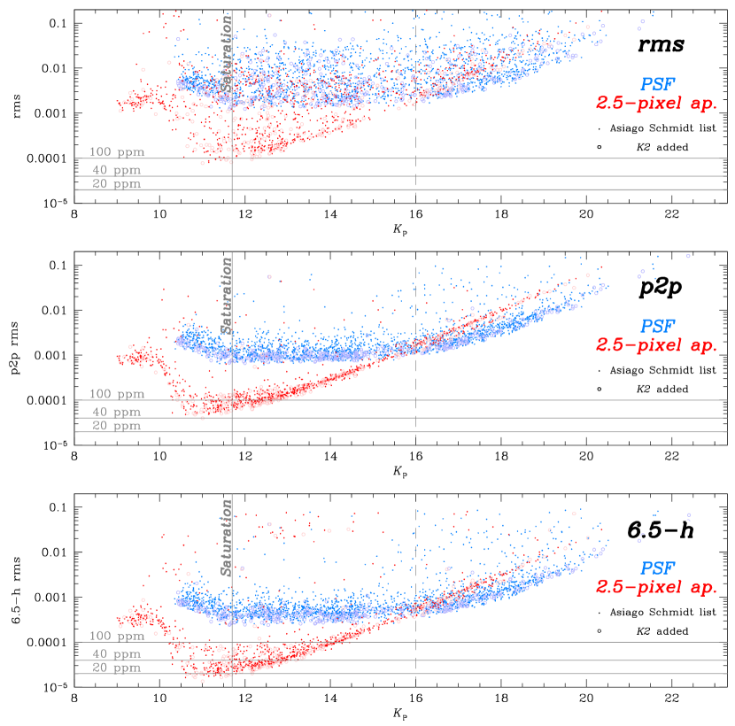
In Fig. 2 we show the 6.5-h rms (defined as in Paper I, ) for each of the four analysed channels. Thanks to observations achieved with a lower spacecraft jitter, the pixel-to-pixel variations are less effective and the photometric precision was slightly better than in Paper I, with a best value of $\sim$13 parts-per-million (ppm). The $K_{\rm P}$ instrumental magnitudes were registered onto the $K_{\rm P}$ system with zero-points (one for each channel and LC-extraction photometric method) obtained by comparing our LC-based $K_{\rm P}$ instrumental magnitudes with the EPIC (Ecliptic Plane Input Catalog) ‘gri’-based $K_{\rm P}$ magnitudes (Paper I).

As it is clear from Fig. 2, the PSF-based photometry (as well as the 1-pixel aperture photometry) is more suitable for faint stars with $K_{\rm P}\gtrsim 17$. This threshold is set $\sim 1.5$ $K_{\rm P}$ magnitudes lower than in Paper I. However, by only focusing on the 2.5-pixel-aperture (the largest aperture adopted in this work) and the PSF photometry, the threshold at which one method overcomes the other is at about $K_{\rm P}\sim 16$, similar to that found in our first work. In Fig. 3 we show the simple rms, the p2p rms and the 6.5-h rms for the 2.5-pixel-aperture and the PSF photometry in which we collected all module-14 LCs.

In Fig. 3 we also marked with different symbols stars included in the original AIC and those that were added to cover the remaining TPFs outside the AIC FoV. No clear dichotomy arises from the plot, meaning that our photometric calibrations while building the mAICs, as well as the registration onto the $K_{\rm P}$ system, are good.

Figure 3: Photometric rms (top panel), p2p rms (middle panel) and 6.5-h rms (bottom panel) for the 2.5-pixel-aperture- (red points) and the PSF-based (azure points) neighbour-subtracted LCs of the four module-14 channels together. Stars contained in the original AIC are shown with dots, while stars added from K2 observations are plot with open circles and a lighter colour. The saturation threshold is set at $K_{\rm P}\sim 11.7$ (grey, solid vertical line). The 100-, 40-, and 20-ppm levels are shown with grey, solid horizontal lines. The grey, dashed vertical line at $K_{\rm P}\sim 16$ shows where one of the two methods begins to perform better than the other.

4 Variable-star search

To find variable stars (e.g., spot-modulated and pulsating stars, eclipsing binaries, transiting objects), we started by selecting for each star the LC among the five obtained with the different photometric methods that shows, on average, the best 6.5-hour rms in the corresponding magnitude interval. Thruster-jet-related events were purged from the LC as in Paper I, while outliers were removed by performing an asymmetric $\sigma$ clipping.

We searched for variable stars using VARTOOLS v1.33 of Hartman & Bakos (2016). The periodograms were obtained with three different methods: Generalized Lomb-Scargle (GLS, Press et al., 1992; Zechmeister & Kürster, 2009), Analysis of Variance (AoV, Schwarzenberg-Czerny, 1989) and Box-fitting Least-Square (BLS, Kovács, Zucker, & Mazeh, 2002). To detect variable-star candidates, we first made an histogram of the periods of all the analysed LCs and removed the spikes that are associated with spurious signals such as thruster-jet firing or other systematic effects. For GLS and AoV, we then plotted the SNR as a function of the period and selected by hand stars that show an high SNR. For BLS we used the signal-to-pink noise (Pont, Zucker, & Queloz, 2006) instead of the SNR. A complete description of the method, supplied with figures, is available in Nardiello et al. (2015) and Paper I.

Among the 2199 field and cluster stars for which we extracted a reliable LC, 1654 objects present a variability signature. As in Paper I, we classified them (by eye comparing the LC of each candidate with those of the close-by neighbours) in three distinct groups: stars that have a high-probability to be true variable sources, eclipsing binaries and candidate exoplanets (1494 stars), probable blends (33 stars) and objects that were difficult to judge just looking at the LC (127 stars). In the latter group there are true variables, blends and stars for which long-term or residual systematic effects could be confused for variability (and vice versa).

4.1 Cross-match with the literature

To estimate the completeness of our variable catalogue, we matched our mAICs with several already-published catalogues focused on M 44. The works considered in our analysis are the following: Agüeros et al. (2011), Bouvier et al. (2001), Breger et al. (2012), Casewell et al. (2012), Delorme et al. (2011), Douglas et al. (2014), Drake et al. (2014), Kovács et al. (2014), Li (2007), Liu et al. (2007), Mermilliod, Mayor, & Udry (2009), Pepper et al. (2008), Samus et al. (2007-2015, GCVS), Scholz et al. (2011), and the “Variable Star Index” (VSX) catalogue.

Of the 1621 (1494 candidate and 127 “difficult-interpretation”) variables we have found, 550 objects were contained in other catalogues. Additional 72 already-known variables were imaged on a TPF during K2/C5 but were not included in our catalogue, therefore we visually inspected again these remaining objects and chose whether to add them or not to our list. In total we added 26 of these missing stars. The remaining 46 already-known variables were not included in our catalogue for different reasons. The missing stars (i) are heavily saturated in these long-cadence images, (ii) are too close to the TPF boundaries or to a very saturated star, (iii) are not included in our mAICs, and/or (iv) do not show any variability in the LC (some objects are listed in catalogues based on spectroscopic/RV observations, therefore we may not be able to detect any variability/binary signature in their LCs).

In total we found 1071 (954 candidate and 117 “difficult-interpretation”) new variables in this M 44 field. We emphasise that, as discussed above and in Sect. 3.2, some long-term systematics left after our detrending may be wrongly interpreted as long-term variability, and hence the new-candidate list could be shorter. Therefore, 1071 should be considered as an indicative value.

Figure 4: From left to right. First column: $B$ versus ($B-K_{\rm 2MASS}$) CMD of the stars in the mAICs. We split the CMD in eight 2.5-magnitude bins (defined by the horizontal, grey dashed lines) to better select the cluster members using PPMXL proper motions. Second column: vector-point diagrams for each magnitude bin. The M 44 members distribution is centred around ($-37.47,-13.39$) mas yr^-1. Field (grey dots) and cluster (black dots) stars were selected accordingly to their location (outside or inside, respectively) with respect to the red circles centred on the M 44 distribution. The radius of these circles ranges from a minimum of 8 mas yr^-1 to a maximum of 10 mas yr^-1. Third column: same CMD as on the first column but with stars plot colour-coded as in the previous vector-point diagrams. Thanks to our proper-motion-based selection, we are able to clearly separate cluster from field stars. Fourth column: CMD with only field stars in which we highlighted the detected candidate variables (green crosses), the “difficult-interpretation” objects (orange dots) and the blends (red triangles). Fifth column: as in the fourth column but for M 44 members.

4.2 CMDs and vector-point diagrams

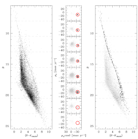
After the cross-match with the literature, we have a catalogue with 1680 stars: 1520 candidate variables, 127 “difficult-interpretation” objects and 33 blends. In Fig. 4 we show the $B$ vs. ($B-K_{\rm 2MASS}$) colour-magnitude diagrams (CMDs) and the vector-point diagrams of the stars observed in our mAICs (for which we have a PPMXL-proper-motion, a $B$- and a $K_{\rm 2MASS}$-magnitude value). The proper-motion selections were made similarly as in Libralato et al. (2015). First, we divided the CMD in eight 2.5-magnitude bins and, for each of such bin, we drew a circle in the corresponding vector-point diagram to select only stars with a cluster-like motion. The adopted radius was chosen as a compromise between excluding cluster members with poorly-measured proper motions and including field stars lying in the cluster-bulk locus. Among the variables in our catalogue with a proper-motion measurement, we found that $\sim$32% of them have a high-probability to be cluster members, while the remaining $\sim$68% of the stars belong to the field in the direction of M 44.

4.3 Peculiar objects

In our analysis we have found two peculiar objects that are worth to be mentioned. In the following subsections we briefly describe them.

4.3.1 LC # 24092 - Channel 45

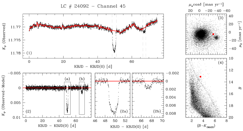
Star # 24092 - 45 (EPIC 211892898) is an eclipsing or transiting field object with a period greater than 50 d. By adopting the stellar parameters given by the K2 EXOFOP website, this object is an eclipsing binary for which we can detected only one primary and one secondary eclipse, and therefore it may have an eccentric orbit. The primary-eclipse depth is of $\sim$0.085 $K_{\rm P}$ magnitude, while the secondary eclipse has a depth of $\sim$0.002 $K_{\rm P}$ magnitude. As shown in Fig. 5 the eclipses last for about two days, suggesting that the system is almost edge-on, with the two components that have a large radii difference and/or that are far from each other. The hypothesis of a grazing eclipsing binary with a large eccentricity cannot be discarded as well.

If the true mass and radius of the star are different than EXOFOP values, a possible interpretation is that we are looking at a planetary system. A RV follow-up is required in order to shed light on the true nature of this object.

4.3.2 LC # 24175 - Channel 46

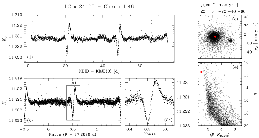
Star # 24175 - 46 (EPIC 211896553) is a potential eccentric binary known as heartbeat binary (e.g., Thompson et al., 2012) not member of M 44. The heartbeat shape in the LCs of these objects is due to tidal distortion of the star after a fly-by at the periastron that changes its brightness. These rare systems (173 heartbeat stars currently known) are characterised by large eccentricities and periods between a fraction of day and $\sim$450 d (see Kirk et al., 2016). Our detected binary has a period of $\sim$27.3 d (Fig. 6). RV measurements are required to constrain the orbital parameters and model the system.

Figure 5: Overview of star # 24092 in channel 45 (EPIC 211892898). In panel (1) we show the original, detrended 2.5-pixel-aperture LC. The red line represents the LC model obtained using a running-median filter with window of 6 hours. The two eclipses/transits (between the grey, dashed, vertical lines) were excluded during the LC modelling. In panel (2) we show the difference between observed and model LCs. Panels (2a) and (2b) highlight the two supposed eclipses/transits. Finally, on the right panels we show the vector-point diagram (panel 3) and the $B$ vs. ($B-K_{\rm 2MASS}$) CMD (panel 4). The red dot marks the location of star # 24092 - 45 in each panel.

Figure 6: Overview for the star # 24175 in channel 46 (EPIC 211896553). On the left panels we plot the original, detrended 2.5-pixel-aperture LC (panel 1), the phased LC with a period of $\sim$27.3 d (panel 2) and a zoom-in around the heartbeat (panel 2a). In panels (3) and (4) we show the vector-point diagram and the $B$ vs. ($B-K_{\rm 2MASS}$) CMD, respectively. Similarly to Fig. 5, in the right panels the red dot marks the location of star # 24175 - 46.

5 Exoplanet search

We searched for candidate exoplanets in M 44 field. To this purpose, we applied a specific procedure that can be summarised as follows.

For each LC, we initially modelled all residual long-term systematic effects and intrinsic variability of the star using a 3^th-order spline with 150 break points and subtracted such model from the LC. We also removed the most of the outliers with an iterative $\sigma$ clipping. Hereafter, we will label the model-subtracted LCs as “flattened” LCs.

For each flattened LC, we extracted the periodogram using VARTOOLS BLS task (searching for periods between 0.5 and 75 d) and normalised it as done by Vanderburg et al. (2016) to decrease the number of false detections in the long-period regime of the spectrum. We then iteratively selected the five peaks with the highest SNR, every time excluding from the subsequent selection all harmonics with $P=N\cdot P_{{\rm sel}}$ and $P=1/N\cdot P_{{\rm sel}}$, $N$ integer. We also avoided to include spurious frequencies (e.g., those related to the spacecraft jitter) in our selection.

For each selected period $P_{\textrm{sel},i=1,...,5}$, we searched for a significant flux drop in the flattened LC. First, we run VARTOOLS BLS, this time fixing the period to refine the central time and the duration of the possible transit. We then phased the flattened LC, computed the median magnitude at the centre of the transit (we used only points within a half of the transit duration centred at the mid-transit time) and checked whether this value was at least 1 $\sigma$ (defined as the 68.27^th percentile of the distribution around the median) below the out-of-transit level or not. If it was not, we discarded the candidate. Next, we verified that the flux drop found was not due to some outliers by comparing the median magnitude at the centre of the transit with and without considering any point within 1 $\sigma$ from the out-of-transit level. If the two values were comparable, the flux drop was real. Finally, we investigated if the examined period was correct or not, by checking for similar flux drops at different phases in the folded flattened LC. For this exoplanet search we chose to also rely on diagnostics other than those provided by BLS because, by setting a selection threshold based on BLS outputs alone, we could exclude good candidates with very shallow transits and noisy LCs, as well as include too many false detections (e.g., eclipsing binaries or RR-Lyrae stars) with high SNR in BLS.

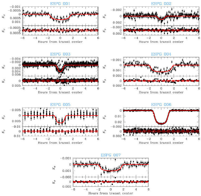
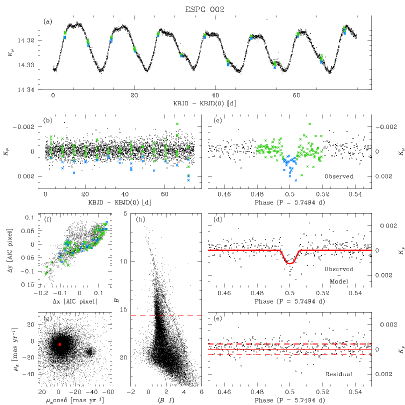
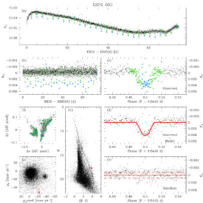
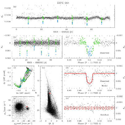
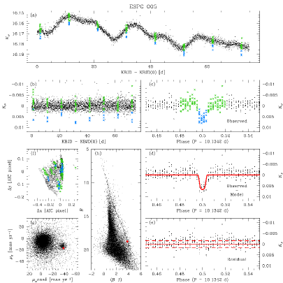
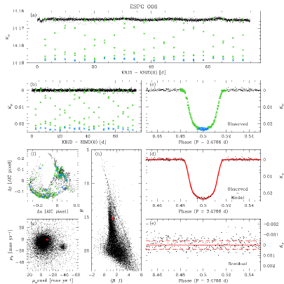
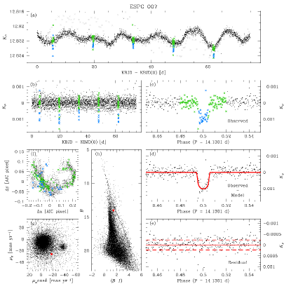
We also double-checked the goodness of the five periods by performing the same analysis described above using multiples ($N$$=$2,3,4) and sub-multiples ($N$$=$$1/2$,$1/3$,$1/4$) of $P_{\textrm{sel},i=1,...,5}$ to take into account that one of the selected peaks could actually be an harmonic of the true period. In total, we explored 35 periods per LC. All stars that passed the aforementioned criteria for one out of the 35 selected periods were visually inspected in their phased LCs and eventually selected for the final candidate sample. In total we detected seven transiting exoplanet candidates. An overview of the candidates is presented in Fig. 7. Single-transit objects were not considered in our analysis.

Figure 7: Overview of the seven exoplanet candidates discovered in this work. For each candidate, on top we plot the phased flattened LC (black dots) with the corresponding model (red solid line) obtained as described in Sect. 5.1. The size of the error bars are computed as the 68.27^th percentile of the distribution of the out-of-transit points around the median. On bottom we show the difference between data and model. The horizontal, red solid line is set at 0, while the two horizontal, red dashed lines are set at $\pm$68.27^th percentile of the distribution of the residuals around the median.

5.1 Vetting and modelling

To verify the goodness of the seven candidates, we first visually inspected the LCs of the variable stars within 100 Kepler pixels from each candidate to search for possible eclipsing binaries miming the transit event and found that these candidates are sufficiently isolated.

We then investigated a possible correlation between transit events and stellar position. To this task, we cannot use the position of the star in the raw-image reference frame because of the Kepler pointing jitter that moves the stars on the CCD and harms the true comprehension of any possible correlation between the transit event and the star location. Therefore we needed an “absolute” reference frame in which we can safely compare the positions and we chose that of the mAIC. The position of the star in the mAIC reference-frame system at each epoch was computed as follows. In each K2/C5 image, we subtracted all close-by neighbours to the exoplanet candidate as done during the LC extraction. We then estimated the position of the star by PSF fitting and transformed it onto the mAIC reference frame by inverting the six-parameter, global linear transformations adopted during the LC extraction (see Sect. 3.2). Within the transformation and the geometric-distortion errors, for our seven candidates no clear correlations arise (panel f in Fig. 8, 9, 10 and 11).

After these validations, we fitted a transit model to extract the transit parameters of these candidates. In order to have a preliminary estimate, we combined the particle-swarm algorithm Pyswarm with the Mandel & Agol (2002) model implemented in PyTransit (Parviainen, 2015), and used the emcee algorithm (Foreman-Mackey et al., 2013) to compute the corresponding errors. For each candidate we adopted the stellar parameters (mass and radius) provided by Huber et al. (2016), retrieved from the K2 EXOFOP website.

We started by purging the most of the outliers from the flattened LCs in order to avoid to model spurious artefacts. We adopted three different methods, tailored for each candidate, to obtain the best purged LC for the subsequent analysis: (i) we subtracted a crude transit model and performed a 3-, 5- or 10-$\sigma$ clipping in the observed-minus-model plane; (ii) we selected only transit neighbourhoods and discarded the off-transit parts of the LC; (iii) we combined the previous two approaches.

In our transit modelling we made some assumptions. We fixed the eccentricity ($e$) and the argument of pericentre ($\omega$) to 0 and 90 deg, respectively. For the limb darkening, we chose a quadratic law and computed the linear and quadratic coefficients with JKTLD (Southworth, 2008) that makes use of the table of Sing (2010). As input for JKTLD, we adopted $T_{\rm eff}$, $\log g$ and [M/H] released in EXOFOP, while the microturbolence velocity was fixed at 2 km s^-1.

The only values that we chose to characterise were the period ($P$), the mid-transit time of reference ($T_{0}$), the inclination ($i$) and the radii ratio ($R_{\rm P}/R_{\rm S}$). For each parameter, we set specific limit values within which to search for the best estimate. We defined $P$ and $T_{0}$ boundaries around guess values obtained by running VARTOOLS BLS. The inclination and the radii ratio were allowed to span a wide range of values, between 70 deg and 110 deg for $i$ and between $10^{-4}$ and $0.5$ for $R_{\rm P}/R_{\rm S}$.

Once set the parameter limits, we let the Pyswarm algorithm span within the boundaries with 180 different parameter configurations for 10 000 iterations. We evaluated the goodness of the fit as the reduced chi-square:

$$\chi^{2}_{\textrm{r}}=\frac{\chi^{2}}{\rm dof}=\sum_{j=1}^{N}{\left(\frac{O_{j}-M_{j}}{\sigma_{O}}\right)}\cdot\frac{1}{\rm dof}\ ,$$ (1)

where $j=1,...,N$ with $N$ number of data points in the LC, $O_{j}$ and $M_{j}$ are the observed and the model data-point value, $\sigma_{O}$ is the associated error equal to the intrinsic dispersion of the flattened LC, and “dof” means degrees of freedom (the difference between the number of data points and the number of fitting parameters). Then, we took the 60 best combinations to initialise the walkers for the emcee algorithm. For each fitting parameter we used uniform priors within the same boundaries defined in Pyswarm. We let the 60 walkers evolve for 40 000 steps, maximising the log-likelihood defined as:

$$\ln\mathcal{L}=-\frac{\chi^{2}}{2}\ .$$ (2)

The best parameters were computed as the median values of the posterior distributions after conservatively discarding as burn-in phase the first 10 000 steps to ensure the convergence of the chains. The related errors were defined as the 68.27^th percentile of the absolute residuals with respect to the median of the posterior distributions of the fitted parameters.

In Table 2 we list all parameters obtained by our LC modelling. Again, we emphasise that our model is strongly dependent on the (fixed) stellar parameter we adopted. A more-reliable estimate of the exoplanet parameters may be obtained after a RV follow-up (at least for the brightest targets). As reference, we also report the photometric transit depth $\delta_{\rm Phot}$. This value was computed as follows. We normalised the LC by its median flux and phased it using the period given by our previous analysis. We set the transit centre at $\rm Phase=0.5$ and computed $\delta_{\rm Phot}$ as the median value of the points with $\lvert\rm Phase-0.5\rvert<0.004$. The related error was computed as:

$$\sigma_{\rm\delta_{Phot}}=\sqrt{\frac{\sigma_{\rm in}^{2}}{\sqrt{N_{\rm in}-1}}+\frac{\sigma_{\rm out}^{2}}{\sqrt{N_{\rm out}-1}}}\ ,$$ (3)

where $\sigma_{\rm in}$ and $\sigma_{\rm out}$ are the 68.27^th percentile of the distribution around the median for the points in ($\lvert\rm Phase-0.5\rvert<0.004$) and out of transit, and $N_{\rm in}$ and $N_{\rm out}$ are the number of points used in the calculation.

Table 1: Exoplanet-candidate parameters.

Candidate	EPIC	R.A.	Dec.	$K_{\rm P}$	Period	$T_{0}$	$i$	$R_{\rm P}/R_{\rm S}$	$\delta_{\rm Phot}$	$R_{\rm S}$	$R_{\rm P}$
		[deg]	[deg]		[d]	[KBJD]	[deg]		[%]	[$R_{\odot}$]	[$R_{\rm Jup}$]
ESPG 001	211913977	130.34349	$+18.934026$	12.646	$14.675828\pm 0.000670$	$2319.686540\pm 0.001737$	$89.26\pm 0.07$	$0.0233\pm 0.0004$	$0.0638\pm 0.0033$	0.725	0.165
ESPG 002	211897691	130.08191	$+18.693113$	14.323	$\phantom{0}5.749481\pm 0.000240$	$2309.495219\pm 0.001717$	$86.89\pm 0.04$	$0.0351\pm 0.0013$	$0.0753\pm 0.0091$	0.765	0.261
ESPG 003	211924657	130.02655	$+19.092411$	15.048	$\phantom{0}2.644259\pm 0.000047$	$2309.002608\pm 0.000650$	$90.00\pm 0.12$	$0.0563\pm 0.0005$	$0.3274\pm 0.0167$	0.225	0.123
ESPG 004	211919004	129.77680	$+19.010098$	13.135	$11.722228\pm 0.000439$	$2316.084281\pm 0.001422$	$90.00\pm 0.09$	$0.0308\pm 0.0002$	$0.1296\pm 0.0055$	0.799	0.240
ESPG 005	211916756	129.36243	$+18.976653$	16.172	$10.134231\pm 0.000347$	$2317.876813\pm 0.001248$	$90.00\pm 0.06$	$0.0713\pm 0.0010$	$0.5276\pm 0.0241$	0.226	0.157
ESPG 006	211929937	129.17834	$+19.173816$	14.165	$\phantom{0}3.476633\pm 0.000006$	$2309.412293\pm 0.000074$	$87.74\pm 0.01$	$0.1341\pm 0.0001$	$2.0868\pm 0.0098$	0.865	1.130
ESPG 007	212008766	129.28246	$+20.399322$	12.822	$14.130142\pm 0.000844$	$2312.117423\pm 0.002062$	$89.44\pm 0.13$	$0.0278\pm 0.0004$	$0.0942\pm 0.0040$	0.794	0.215

• Notes. $K_{\rm P}$ is the median magnitude in the LC. Period, $T_{0}$, $i$ and $R_{\rm P}/R_{\rm S}$ were computed as described in the text. $T_{0}$ is referred at the first, clearest transit event in the LC, therefore it may not coincide with the first transit event in the K2/C5. The stellar radius $R_{\rm S}$ is taken from Huber et al. (2016). $R_{\rm P}$ is derived using $R_{\rm P}/R_{\rm S}$.

Table 2: Our independent estimates of the planetary parameters of the two M 44 transiting exoplanet candidates discovered by Pope, Parviainen, & Aigrain (2016) in K2/C5 module 14.

EPIC	R.A.	Dec.	$K_{\rm P}$	Period	$T_{0}$	$i$	$R_{\rm P}/R_{\rm S}$	$\delta_{\rm Phot}$	$R_{\rm S}$	$R_{\rm P}$
	[deg]	[deg]		[d]	[KBJD]	[deg]		[%]	[$R_{\odot}$]	[$R_{\rm Jup}$]
211969807	129.63691	$+19.773718$	15.381	$\phantom{0}1.974172\pm 0.000089$	$2307.382086\pm 0.001830$	$88.75\pm 0.45$	$0.0297\pm 0.0012$	$0.1008\pm 0.0125$	0.303	0.088
211990866	129.60134	$+20.106105$	10.370	$\phantom{0}1.673918\pm 0.000060$	$2341.197012\pm 0.000776$	$76.72\pm 0.09$	$0.0273\pm 0.0007$	$0.0621\pm 0.0096$	1.572	0.417

• Notes. See notes in Table 2.

5.2 Field and M 44 candidates description

For each exoplanet candidate, in Fig 8, 9, 10 and 11 we provide different plots summarising the results. Adopting for the host stars the radius values given by EXOFOP, if these signals correspond to bona-fide planets we have detected one hot Jupiter (ESPG 006) and six smaller (a few $R_{\earth}$) planets.

Five out of seven objects (ESPG 002, ESPG 003, ESPG 004, ESPG 006 and ESPG 007) are hosted by a field star, while the remaining two candidate (ESPG 001 and ESPG 005) hosts are probable members of M 44 (on the basis of their PPMXL proper motions and CMD locations). For these two candidate exoplanets, a RV follow-up would be particularly important. Therefore, under simple assumptions, we can attempt to derive indicative estimates of their expected RV signals, and assess whether a RV follow-up is feasible or not with today’s facilities.

Planetary radii (estimated using the parameters listed in Table 2) of our two candidates were converted into indicative masses by using the probabilistic mass-radius relationship of Wolfgang, Rogers, & Ford (2015) and its public-available code. We used the coefficients obtained from RV-based masses of planets with $R<4R_{\earth}$. Confidence intervals were determined by taking the 15.865^th and the 84.135^th percentiles of the posterior distributions, although their upper limits are set by the maximum density allowed for a rocky planet (Fortney, Marley, & Barnes, 2007). We obtained $M=(5.9\pm 2.3)M_{\earth}$ (upper limit at 7.3 $M_{\earth}$) for ESPG 001 and $M=(5.6\pm 2.3)M_{\earth}$ (upper limit at 6.9 $M_{\earth}$) for ESPG 005. Using these planetary masses, the periods of the planets and their inclination with respect to the line of sight obtained from the previous LC analysis (Table 2), and assuming circular orbits, we expect a RV semi amplitude of $K=(1.8\pm 0.7)$ m s^-1 (upper limit to 2.2 m s^-1) for ESPG 001 and $K=(4.6\pm 1.9)$ m s^-1 (upper limit to 5.6 m s^-1) for ESPG 005.

Figure 8: Summary plots for the two exoplanet candidates ESPG 001 and ESPG 002. For each candidate, the detrended and the flattened LCs are shown in panel (a) and (b), respectively. The phased LC is presented in panel (c). Grey crosses represent LC points excluded from the analysis (e.g., thruster-jet-related events, outliers or noisy parts at the beginning of the LC). The centre of the transit is set at 0.5 phase by construction. We marked with azure crosses the points with $\lvert\rm Phase-0.5\rvert<0.004$. These points roughly map the centre of the transit in the phased LC. Green crosses highlight the remaining transit points from before the ingress to after the egress of the transit ($0.004<\lvert\rm Phase-0.5\rvert<0.02$). In panel (d) we show again the phased LC and the corresponding model (red solid line) obtained as described in Sect. 5.1. In panel (e) the difference between the observed data and the model is presented. The horizontal, red solid line is set at 0; while the horizontal, red dashed lines are set at the 68.27^th percentile of the distribution of these residuals around the median. In panel (f) we show the star displacements in the corresponding mAIC reference-frame system. The colour-coding scheme is the same as that adopted in the previous panels. Note that the ($\Delta x$,$\Delta y$) displacements are in AIC pixels (1 Asiago Schmidt pixel $\sim 0.2$ K2 pixel). Finally, in panel (g) and (h) we show the vector-point diagram and the $B$ vs. ($B-I$) CMD for the stars in the original AIC, respectively. The location of the exoplanet candidate is highlighted with a red dot. Since we do not have a $B$- and a $I$-filter magnitude entry for ESPG 002 in our AIC, we drew as a reference a horizontal, red dashed line in the CMD using EXOFOP $B$-magnitude value.

Figure 9: Same as in Fig. 8 but for ESPG 003 and ESPG 004 candidates. For ESPG 003, in panel (g) we marked with an arrow the location of the star because it lies outside the vector-point-diagram boundaries ($\mu_{\delta}=-132.6$ mas yr^-1).

Figure 10: Same as in Fig. 8 and 9 but for ESPG 005 and ESPG 006 candidates.

Figure 11: Same as in Fig. 8, 9 and 10 but for ESPG 007 candidate.

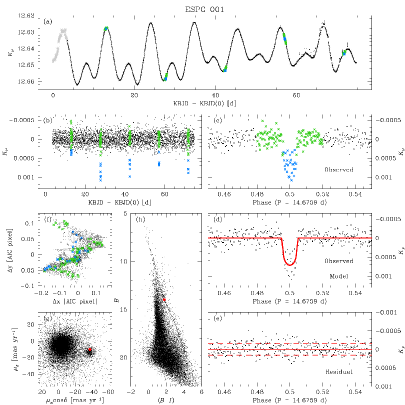
With the aim of obtaining an independent estimate of the host-star masses and radii than those given by EXOFOP, we used our photometry and a PARSEC (PAdova Trieste Stellar Evolution Code) isochrone (see Bressan et al., 2012; Rosenfield et al., 2016, and reference therein) to derive these parameters. While for ESPG 001 the values are in rather good agreement, for ESPG 005 we found a mass and a radius double than EXOFOP parameters. We repeated the entire analysis for this candidate with the new stellar mass and radius values and found a new expected RV semi amplitude of $K=(6.1\pm 0.3)$ m s^-1 (upper limit to 6.8 m s^-1).

Either way, with the available facilities (e.g., HARPS-N@TNG), the faintness ($V\sim 17.27$) of ESPG 005 precludes its complete characterisation. Therefore, the only cluster-hosted exoplanet candidate for which a RV follow-up is possible, but challenging, remains ESPG 001.

The presence of spots and flares on the stellar surface are the main responsible of the photometric modulation seen in stars of young and intermediate-age clusters such as Praesepe. The same physical process is affecting spectroscopic observations, and as a consequence RV variations not due to a physical movement of the star are observed (the so-called RV jitter). The RV jitter in M 44 and in the almost-coeval Hyades cluster is around 15 m s^-1 (Paulson, Cochran, & Hatzes, 2004; Quinn et al., 2012). Such RV jitter could lower the sensitivity of RV measurements to low-mass planets. However, thanks to the common origin of RV jitter and photometric modulation, several works have shown that when the rotational period of the star is known (from photometry) it is possible to model and correct for the activity-induced RV variations. This result can be achieved if a proper observing strategy, that allows to sample both the rotational period of the star and the period of the planets, is implemented. A variety of successful techniques have been developed in this direction (see for example Boisse et al., 2011; Haywood et al., 2014; Faria et al., 2016; Malavolta et al., 2016).

5.3 Literature on exoplanets in M 44

During a RV survey focused on M 44, Quinn et al. (2012) found two hot Jupiters and later, around one of these two stars, Malavolta et al. (2016) also discovered (always with RV measurements) another exoplanet. We checked the LCs of these stars but none of them showed any transit signature. We also checked all candidates surveyed by Quinn et al. (2012) and again found a null detection. Pepper et al. (2008) found two candidates exoplanets in M 44 field. However, accordingly to their PPMXL proper motions, none of them is member of M 44.

About K2, Adams, Jackson, & Endl (2016) searched for ultra-short-period ($P<1$d) planets from Campaign 0 to 5. Only one of their candidates (EPIC 211995325) was observed on a module-14 TPF. The object was not detected by our pipeline because we do not search for periods shorter than 0.5 d and the transit depth did not satisfy our selection criteria (see Sect. 5).

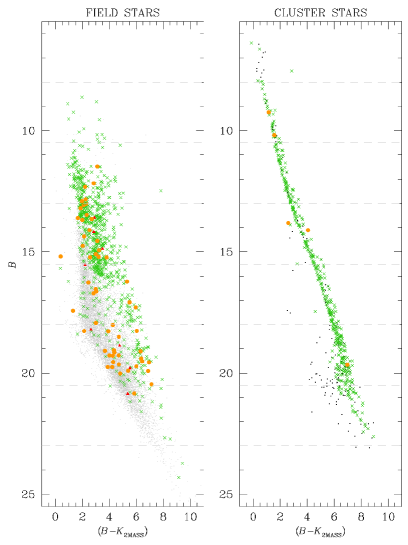
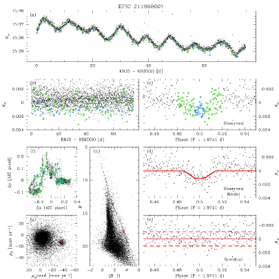
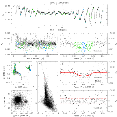
At the time of our submission, a work by Pope, Parviainen, & Aigrain (2016) presenting an independent reduction of the same K2/C5 data was published. These authors found 10 exoplanet candidates within the same K2 module 14 analysed in our work. Five of them were also discovered by our pipeline (namely, ESPG 002, ESPG 003, ESPG 004, ESPG 006 and ESPG 007). The remaining five objects were missed because we did not detect any significant transit signature in our LC or the transit depth was not $1\sigma$ below the out-of-transit level, one of the requirements in our exoplanet finding. Accordingly to their CMD and vector-point-diagram locations, two of such missed candidates (EPIC 211969807 and EPIC 211990866) are M 44 members with high probability (see Table 2 and Fig. 12). Note that EPIC 211990866 is saturated in K2 exposures and its LC has a low photometric precision, which may explain why we failed to identify it. We note that two of our candidates (those hosted by M 44 stars, ESPG 001 and ESPG 005) were not detected Pope, Parviainen, & Aigrain (2016). This is an additional evidence that in general every K2 data reduction pipeline has its pro’s and con’s and still needs improvements (e.g., as done for the Kepler main mission).

Nevertheless, we will add these missing candidates (at least those clearly visible in our LCs) to the final variable and exoplanet catalogue we are going to release with this paper (see Sect. 6).

6 Electronic material

With this work we release all raw and detrended LCs for 1-, 1.5-, 2- and 2.5-pixel aperture and PSF photometry obtained from the neighbour-subtracted images. We also release the K2 astrometrised stacked images of the four module-14 channels.

We released a single catalogue that is the merge of the four mAICs. We chose to merge them to simplify their usage. The catalogue is made as follows (see Table 4). Columns (1) and (2) give the J2000.0 equatorial coordinates in decimal degrees. Columns from (3) to (9) provide the $N$$B$$R$$I$$J_{\rm 2MASS}$$H_{\rm 2MASS}$$K_{\rm 2MASS}$ calibrated (except for the $N$-filter photometry) magnitudes, when available (otherwise flagged to $-99.9999$). PPMXL ($\mu_{\alpha}\cos\delta$,$\mu_{\delta}$) proper motions are listed in columns (10) and (11). We set the column values to $-999.99$ if the proper motions were not available. In column (12) we give the instrumental $K_{\rm P}$ of the corresponding mAIC obtained as described in Sect. 3.1. Finally in columns (13) and (14) we provide the ID of the star in the corresponding mAIC and the number of the K2 channel in which the star was imaged. These two columns univocally identify the LC of the star (particularly important for the stars added to the original AIC, see Sect. 3.1). For stars outside any K2 channel, column (14) value was set at 0 and $K_{\rm P}$ to $-99.9999$.

For the variable stars and exoplanet candidates we detected, we provide to the community a catalogue with the following columns. Column (1) gives the ID of the star in the mAIC catalogue, while column (2) contains the channel in which the star was imaged. Columns (3) provides the $K_{\rm P}$ magnitude, obtained from the LC as described in Sect. 3.3. In column (4) we list the variable periods, when available (e.g., for irregular or long-period variables we set it at the K2/C5 duration). Column (5) contains the flag of our by-eye classification:
$\bullet$ 1: candidate variable;
$\bullet$ 2: “difficult-interpretation” object;
$\bullet$ 3: possible blend.

Finally, in the last column (6) we give some notes about the catalogues in the literature in which it was already described or if the star also hosts an exoplanet candidate.

Figure 12: Summary plots for the two M 44 exoplanet candidates discovered by Pope, Parviainen, & Aigrain (2016) in K2/C5 module 14. See Fig. 8 for a complete description of the panels. Note in panel (f) of EPIC 211990866 that ($\Delta x$,$\Delta y$) displacements can reach more than one Asiago-Schmidt pixel because it is saturated and its position was measured with a low positional accuracy.

7 Conclusions

Exoplanets hosted by cluster stars are of particular interest to shed light on the still-debated questions about their formation and evolution. Indeed, stellar parameters (such as distance, chemistry, mass, and age) are generally determined with a much higher accuracy for stars in cluster rather than those in the Galactic field, giving in return better-constrained exoplanet parameters. Furthermore, stellar clusters are composed by an ensemble of stars with similar properties, and such characteristic can enable a variety of investigations, e.g, we can search for the presence of a relation between exoplanets and host masses, understand the importance of the dynamical evolution, or simply perform comparative analyses between cluster stars with and without planets.

In this work we present our attempt to detect transiting exoplanet candidates in the OC M 44 using K2/C5 data. M 44 is one of the few star clusters where the presence of exoplanets was firmly confirmed with RV measurements (Quinn et al., 2012; Malavolta et al., 2016).

We applied our PSF-based techniques (starting from the work presented in Paper I, and improving it) to extract high-photometric-precision and less-neighbour-contaminated LCs for the stars imaged on a given module-14 TPF during K2/C5. As main result of this effort, we detected seven transiting exoplanet candidates, one hot Jupiter and six smaller planets. Two of our candidates (ESPG 001 and ESPG 005) seems to be hosted by M 44 members. Together with those find by Pope, Parviainen, & Aigrain (2016), they set the number of currently-known, transiting exoplanet candidates in M 44 to four objects (Table 5). A RV follow-up confirmation is required to constrain their orbital and physical parameters.

Finally, as by-product of our work, we discovered 1071 new variable stars, tripling the number of known variables in this field to date. Their LCs, together with those of all other objects monitored in module 14 during K2/C5, will be released via our website.

Part of our pipeline (detrending and transit search) is continuously evolving and improving, therefore we release both raw and detrended LCs to allow the community to not only purse their scientific goals, but also to stimulate the development and the improvement of K2 pipelines in general. This work is not a stand-alone struggle, but it will be also very fruitful to promptly analyse the data coming from the next exoplanet-search missions TESS (Transiting Exoplanet Survey Satellite, Ricker et al., 2014) and PLATO (PLAnetary Transits and stellar Oscillations, Rauer et al., 2014).

Table 3: First ten rows of the M 44 input catalogue (merge of the four mAICs) we are going to release as electronic material.

Row	R.A.	Dec.	$N$	$B$	$R$	$I$	$J_{\rm 2MASS}$	$H_{\rm 2MASS}$	$K_{\rm 2MASS}$	$\mu_{\alpha}\cos\delta$	$\mu_{\delta}$	$K_{\rm P}$	ID	K2 Channel
	[deg]	[deg]								[mas yr-1]	[mas yr-1]
	(1)	(2)	(3)	(4)	(5)	(6)	(7)	(8)	(9)	(10)	(11)	(12)	(13)	(14)
1	131.06866	20.82924	$-14.8861$	$-99.9999$	$-99.9999$	$-99.9999$	$12.364$	$12.045$	$12.012$	$3.80$	$-9.00$	$-12.1162$	1	48
2	131.06603	20.76100	$-14.5165$	$-99.9999$	$-99.9999$	$-99.9999$	$12.839$	$12.570$	$12.509$	$0.90$	$-2.30$	$-11.7466$	2	48
3	131.06539	20.37455	$-10.5516$	$-99.9999$	$-99.9999$	$-99.9999$	$16.117$	$15.296$	$15.210$	$-0.90$	$-14.40$	$-7.7817$	3	48
4	131.06347	20.62682	$-13.7107$	$-99.9999$	$-99.9999$	$-99.9999$	$13.098$	$12.654$	$12.504$	$-8.70$	$-3.50$	$-10.9408$	4	48
5	131.06191	20.12612	$-14.1353$	$-99.9999$	$-99.9999$	$-99.9999$	$12.426$	$11.892$	$11.761$	$-14.30$	$-23.80$	$-11.3654$	5	48
6	131.06303	20.98408	$-13.0740$	$-99.9999$	$-99.9999$	$-99.9999$	$13.725$	$13.274$	$13.222$	$-7.60$	$-13.00$	$-99.9999$	6	0
7	131.06130	20.02970	$-12.1400$	$-99.9999$	$-99.9999$	$-99.9999$	$14.847$	$14.548$	$14.513$	$0.00$	$-9.60$	$-9.3701$	7	48
8	131.06210	20.65114	$-13.1195$	$-99.9999$	$-99.9999$	$-99.9999$	$13.990$	$13.665$	$13.555$	$-7.10$	$-5.50$	$-10.3496$	8	48
9	131.06153	20.62936	$-10.6903$	$-99.9999$	$-99.9999$	$-99.9999$	$16.324$	$16.115$	$15.661$	$-3.00$	$-3.40$	$-7.9204$	9	48
10	131.05881	18.94697	$-13.5582$	$-99.9999$	$-99.9999$	$-99.9999$	$-99.9999$	$-99.9999$	$-99.9999$	$-999.99$	$-999.99$	$-10.8129$	10	45
(…)	(…)	(…)	(…)	(…)	(…)	(…)	(…)	(…)	(…)	(…)	(…)	(…)	(…)	(…)

Table 4: First ten rows of the variable/exoplanet catalogue.

Row	ID	K2 Channel	LC $K_{\rm P}$	$P$	Flag	Notes
				[d]
	(1)	(2)	(3)	(4)	(5)	(6)
1	17	45	12.35	11.09064293	1
2	29	45	14.32	14.21546437	1
3	30	45	13.61	12.19786185	1	6, 8
4	45	45	12.21	9.46942449	1
5	59	45	15.65	74.82000000	1
6	119	45	13.52	74.82000000	1
7	267	45	12.05	74.82000000	1	12
8	298	45	13.70	74.82000000	1
9	304	45	16.76	10.42804406	2
10	307	45	16.48	18.14582914	2
(…)	(…)	(…)	(…)	(…)	(…)	(…)

• Notes. Column (6) lists the catalogues in literature that already analysed the object (1 = Agüeros et al. (2011), 2 = Bouvier et al. (2001), 3 = Breger et al. (2012), 4 = Casewell et al. (2012), 5 = Delorme et al. (2011), 6 = Douglas et al. (2014), 7 = Drake et al. (2014), 8 = Kovács et al. (2014), 9 = Li (2007), 10 = Liu et al. (2007), 11 = Malavolta et al. (2016), 12 = Mermilliod, Mayor, & Udry (2009), 13 = Pepper et al. (2008), 14 = Quinn et al. (2012), 15 = Scholz et al. (2011), 16 = GCVS, 17 = VSX) and/or states if the star hosts one of the candidate exoplanets listed in Tables 2 and 2.

Table 5: List of M 44 candidate and confirmed exoplanets.

EPIC	R.A.	Dec.	Notes
	[deg]	[deg]
Candidates
211913977	130.34349	$+18.934026$	ESPG 001
211916756	129.36243	$+18.976653$	ESPG 005
211969807	129.63691	$+19.773718$
211990866	129.60134	$+20.106105$
Confirmed
211998346	130.43243	$+20.226899$	Pr201b
211936827	130.54745	$+19.277061$	Pr211b,c

• Notes. EPIC 211998346 and 211936827 are the two M 44 stars that host the three RV-confirmed exoplanets discovered by Quinn et al. (2012) and Malavolta et al. (2016).

References

- Adams, Jackson, & Endl (2016) Adams E. R., Jackson B., Endl M., 2016, arXiv, arXiv:1603.06488
- Agüeros et al. (2011) Agüeros M. A., et al., 2011, ApJ, 740, 110
- Aigrain, Parviainen, & Pope (2016) Aigrain S., Parviainen H., Pope B. J. S., 2016, MNRAS, 459, 2408
- An et al. (2007) An D., Terndrup D. M., Pinsonneault M. H., Paulson D. B., Hanson R. B., Stauffer J. R., 2007, ApJ, 655, 233
- Anderson & King (2000) Anderson, J., & King, I. R. 2000, PASP, 112, 1360
- Anderson et al. (2006) Anderson J., Bedin L. R., Piotto G., Yadav R. S., Bellini A., 2006, A&A, 454, 1029
- Anderson et al. (2008) Anderson J., et al., 2008, AJ, 135, 2114
- Boisse et al. (2011) Boisse I., Bouchy F., Hébrard G., Bonfils X., Santos N., Vauclair S., 2011, A&A, 528, A4
- Borucki et al. (2010) Borucki W. J., et al., 2010, Sci, 327, 977
- Bouvier et al. (2001) Bouvier J., Duchêne G., Mermilliod J.-C., Simon T., 2001, A&A, 375, 989
- Breger et al. (2012) Breger M., et al., 2012, AN, 333, 131
- Bressan et al. (2012) Bressan A., Marigo P., Girardi L., Salasnich B., Dal Cero C., Rubele S., Nanni A., 2012, MNRAS, 427, 127
- Casewell et al. (2012) Casewell S. L., et al., 2012, ApJ, 759, L34
- Delorme et al. (2011) Delorme P., Collier Cameron A., Hebb L., Rostron J., Lister T. A., Norton A. J., Pollacco D., West R. G., 2011, MNRAS, 413, 2218
- Douglas et al. (2014) Douglas S. T., et al., 2014, ApJ, 795, 161
- Drake et al. (2014) Drake A. J., et al., 2014, ApJS, 213, 9
- Faria et al. (2016) Faria J. P., Haywood R. D., Brewer B. J., Figueira P., Oshagh M., Santerne A., Santos N. C., 2016, A&A, 588, A31
- Foreman-Mackey et al. (2013) Foreman-Mackey D., Hogg D. W., Lang D., Goodman J., 2013, PASP, 125, 306
- Fortney, Marley, & Barnes (2007) Fortney J. J., Marley M. S., Barnes J. W., 2007, ApJ, 659, 1661
- Hartman & Bakos (2016) Hartman J. D., Bakos G. Á., 2016, A&C, 17, 1
- Haywood et al. (2014) Haywood R. D., et al., 2014, MNRAS, 443, 2517
- Howell et al. (2014) Howell S. B., et al., 2014, PASP, 126, 398
- Huber et al. (2016) Huber D., et al., 2016, ApJS, 224, 2
- Kirk et al. (2016) Kirk B., et al., 2016, AJ, 151, 68
- Kovács, Zucker, & Mazeh (2002) Kovács G., Zucker S., Mazeh T., 2002, A&A, 391, 369
- Kovács et al. (2014) Kovács G., et al., 2014, MNRAS, 442, 2081
- Li (2007) Li Z. P., 2007, AJ, 133, 518
- Libralato et al. (2014) Libralato M., Bellini A., Bedin L. R., Piotto G., Platais I., Kissler-Patig M., Milone A. P., 2014, A&A, 563, A80
- Libralato et al. (2015) Libralato M., et al., 2015, MNRAS, 450, 1664
- Libralato et al. (2016) Libralato M., Bedin L. R., Nardiello D., Piotto G., 2016, MNRAS, 456, 1137
- Liu et al. (2007) Liu L., Qian S.-B., Boonrucksar S., Zhu L.-Y., He J.-J., Yuan J.-Z., 2007, PASJ, 59, 607
- Malavolta et al. (2016) Malavolta L., et al., 2016, A&A, 588, A118
- Mandel & Agol (2002) Mandel K., Agol E., 2002, ApJ, 580, L171
- Mermilliod, Mayor, & Udry (2009) Mermilliod J.-C., Mayor M., Udry S., 2009, A&A, 498, 949
- Moré, Garbow, & Hillstrom (1980) Moré J. J., Garbow B. S., Hillstrom K. E., 1980, Technical Report ANL-80-74, User guide for MINPACK-1, Argonne Nat. Lab., Argonne, IL
- Nardiello et al. (2015) Nardiello D., et al., 2015, MNRAS, 447, 3536
- Nardiello et al. (2016) Nardiello D., Libralato M., Bedin L. R., Piotto G., Ochner P., Cunial A., Borsato L., Granata V., 2016, MNRAS, 455, 2337
- Parviainen (2015) Parviainen H., 2015, MNRAS, 450, 3233
- Paulson, Cochran, & Hatzes (2004) Paulson D. B., Cochran W. D., Hatzes A. P., 2004, AJ, 127, 3579
- Pepper et al. (2008) Pepper J., Stanek K. Z., Pogge R. W., Latham D. W., DePoy D. L., Siverd R., Poindexter S., Sivakoff G. R., 2008, AJ, 135, 907
- Pont, Zucker, & Queloz (2006) Pont F., Zucker S., Queloz D., 2006, MNRAS, 373, 231
- Pope, Parviainen, & Aigrain (2016) Pope B. J. S., Parviainen H., Aigrain S., 2016, MNRAS,
- Press et al. (1992) Press W. H., Teukolsky S. A., Vetterling W. T., Flannery B. P., 1992, nrca.book
- Quinn et al. (2012) Quinn S. N., et al., 2012, ApJ, 756, L33
- Rauer et al. (2014) Rauer H., et al., 2014, ExA, 38, 249
- Ricker et al. (2014) Ricker G. R., et al., 2014, SPIE, 9143, 914320
- Roeser, Demleitner, & Schilbach (2010) Roeser S., Demleitner M., Schilbach E., 2010, AJ, 139, 2440
- Rosenfield et al. (2016) Rosenfield P., Marigo P., Girardi L., Dalcanton J. J., Bressan A., Williams B. F., Dolphin A., 2016, ApJ, 822, 73
- Samus et al. (2007-2015) Samus N.N., Durlevich O.V., Goranskij V.P., Kazarovets E. V., Kireeva N.N., Pastukhova E.N., Zharova A.V., General Catalogue of Variable Stars (Samus+ 2007-2015), VizieR On-line Data Catalog: B/gcvs
- Schwarzenberg-Czerny (1989) Schwarzenberg-Czerny A., 1989, MNRAS, 241, 153
- Scholz et al. (2011) Scholz A., Irwin J., Bouvier J., Sipőcz B. M., Hodgkin S., Eislöffel J., 2011, MNRAS, 413, 2595
- Sing (2010) Sing D. K., 2010, A&A, 510, A21
- Southworth (2008) Southworth J., 2008, MNRAS, 386, 1644
- Skrutskie et al. (2006) Skrutskie M. F., et al., 2006, AJ, 131, 1163
- Thompson et al. (2012) Thompson S. E., et al., 2012, ApJ, 753, 86
- Vanderburg & Johnson (2014) Vanderburg A., Johnson J. A., 2014, PASP, 126, 948
- Vanderburg et al. (2016) Vanderburg A., et al., 2016, ApJS, 222, 14
- Wolfgang, Rogers, & Ford (2015) Wolfgang A., Rogers L. A., Ford E. B., 2015, arXiv, arXiv:1504.07557
- Zechmeister & Kürster (2009) Zechmeister M., Kürster M., 2009, A&A, 496, 577