Kernel Risk-Sensitive Loss: Definition, Properties and Application to Robust Adaptive Filtering

Badong Chen, Senior Member, IEEE, Lei Xing, Bin Xu, Member, IEEE, Haiquan Zhao, Member, IEEE
Nanning Zheng, Fellow, IEEE, José C. Príncipe, Fellow, IEEE
Abstract

Nonlinear similarity measures defined in kernel space, such as correntropy, can extract higher-order statistics of data and offer potentially significant performance improvement over their linear counterparts especially in non-Gaussian signal processing and machine learning. In this work, we propose a new similarity measure in kernel space, called the kernel risk-sensitive loss (KRSL), and provide some important properties. We apply the KRSL to adaptive filtering and investigate the robustness, and then develop the MKRSL algorithm and analyze the mean square convergence performance. Compared with correntropy, the KRSL can offer a more efficient performance surface, thereby enabling a gradient based method to achieve faster convergence speed and higher accuracy while still maintaining the robustness to outliers. Theoretical analysis results and superior performance of the new algorithm are confirmed by simulation.

Key Words: Correntropy; risk-sensitive criterion; kernel risk-sensitive loss, robust adaptive filtering.

footnotetext: This work was supported by 973 Program (No. 2015CB351703) and National NSF of China (No. 61372152). Badong Chen, Lei Xing, and Nanning Zheng are with the Institute of Artificial Intelligence and Robotics, Xi’an Jiaotong University, Xi’an, 710049, China.(chenbd; nnzheng @mail.xjtu.edu.cn; xl2010@stu.xjtu.edu.cn). Bin Xu is with the School of Automation, Northwestern Polytechnical University (NPU), Xi’an, China. (binxu@nwpu.edu.cn) Haiquan Zhao is with the School of Electrical Engineering, Southwest Jiaotong University, Chengdu, China. (hqzhao@home.swjtu.edu.cn) José C. Príncipe is with the Department of Electrical and Computer Engineering, University of Florida, Gainesville, FL32611 USA (principe@cnel.ufl.edu), and is also with the Institute of Artificial Intelligence and Robotics, Xi’an Jiaotong University, Xi’an, 710049, China.

I Introduction

STATISTICAL similarity measures play significant roles in signal processing and machine learning communities. In particular, the cost function for a learning machine is usually a certain similarity measure between the learned model and the data generating system. Due to their simplicity, mathematical tractability and optimality under Gaussian and linear assumptions, second-order similarity measures defined in terms of inner products, such as correlation and mean square error (MSE), have been widely used to quantify how similar two random variables (or random processes) are. However, second-order statistics cannot quantify similarity fully if the random variables are non-Gaussian distributed[1, 2]. To address the problem of modeling with non-Gaussian data (which are very common in many real-world applications), similarity measures must go beyond second-order statistics. Higher-order statistics, such as kurtosis, skewness, higher-order moments or cumulants, can be applicable for dealing with non-Gaussian data. Besides, as an alternative to the MSE, the risk-sensitive loss[3, 4, 5, 6, 7], which quantifies the similarity by emphasizing the larger errors in an exponential form (”risk-sensitive” means ”average-of-exponential”), has been proven to be robust to the case where the actual probabilistic model deviates from the assumed Gaussian model[6]. The problem of existence and uniqueness of the risk-sensitive estimation has been studied in [7]. Nevertheless, the risk-sensitive loss is not robust to impulsive noises (or outliers) when utilizing a gradient-based learning algorithm, because its performance surface (as a function over parameter space) can be super-convex and the gradient may grow exponentially fast with error increasing across iterations.

Recent advances in information theoretic learning (ITL) suggest that similarity measures can also be defined in a reproducing kernel Hilbert space (RKHS)[1].The ITL costs (i.e. entropy and divergence) for adaptive system training can be directly estimated from data via a Parzen kernel estimator, which can capture higher-order statistics of data and achieve better solutions than MSE particularly in non-Gaussian and nonlinear signal processing [8, 9, 10, 11, 12, 13, 14]. As a local similarity measure in ITL, the correntropy is defined as a generalized correlation in kernel space, directly related to the probability of how similar two random variables are in a neighborhood of the joint space [15, 16]. The kernel function in correntropy is usually a Gaussian kernel, but it can be extended to generalized Gaussian functions [17]. Since correntropy measures the similarity in an observation window (controlled by the kernel bandwidth), it provides an effective way to eliminate the adverse effects of outliers [1]. So far correntropy has been successfully applied to develop various robust learning or adaptive algorithms [18, 19, 20, 21, 22, 23, 24, 25, 26, 27, 28]. However, the performance surface of the correntropic loss (C-Loss) is highly non-convex, which can be very sharp around the optimal solution while extremely flat at a region far away from the optimal solution, and this may result in poor convergence performance in adaptation [29].

In this paper, we define a new similarity measure in kernel space, called the kernel risk-sensitive loss (KRSL), which inherits the original form of risk-sensitive loss but is defined in RKHS by means of kernel trick. The performance surface of KRSL is bounded but can be more ”convex” than that of C-Loss, leading to a faster convergence speed and higher solution accuracy while maintaining the robustness to outliers. Besides the kernel bandwidth, an extra free parameter, namely the risk-sensitive parameter, is introduced to control the shape of the performance surface. Further, we apply the KRSL to develop a new robust adaptive filtering algorithm, referred to in this work as the minimum kernel risk-sensitive loss (MKRSL) algorithm, which can outperform existing methods, including the recently proposed generalized maximum correntropy criterion (GMCC) algorithm [17]. A brief version of this work was presented at 2015 IEEE International Conference on Digital Signal Processing [30].

The rest of the paper is organized as follows. In section II, after briefly reviewing some background on similarity measures in kernel space, we define the KRSL, and present some important properties. In section III, we apply the proposed KRSL to adaptive filtering and analyze the robustness, and develop the MKRSL algorithm and present the mean square convergence performance. In section IV, we carry out Monte Carlo simulations to confirm the theoretical results and demonstrate the superior performance of the new algorithm. Finally, we give the conclusion in section V.

II KERNEL RISK-SENSITIVE LOSS

II-A Background on Similarity Measures in Kernel Space

The kernel methods have been widely applied in domains of machine learning and signal processing [31, 32, 33].Let κ(x,y)𝜅𝑥𝑦\kappa(x,y) be a continuous, symmetric and positive definite Mercer kernel defined over 𝓧×𝓧𝓧𝓧\boldsymbol{\mathscr{X}}\times\boldsymbol{\mathscr{X}}.Then the nonlinear mapping Φ(x)=κ(x,.)\Phi(x)=\kappa(x,.) transforms the data x𝑥x from the input space to a functional Hilbert space, namely a reproducing kernel Hilbert space (RKHS)H, satisfying f(x)=κ(x,.),fHf(x)={\left\langle{\kappa(x,.),f}\right\rangle_{\textbf{H}}} , fHfor-all𝑓H\forall f\in\textbf{H} , where .,.H{\left\langle{.,.}\right\rangle_{\textbf{H}}} denotes the inner product in H. In particular, we have

κ(x,y)=Φ(x),Φ(y)H=κ(x,.),κ(y,.)H\kappa(x,y)={\left\langle{\Phi(x),\Phi(y)}\right\rangle_{\textbf{H}}}={\left\langle{\kappa(x,.),\kappa(y,.)}\right\rangle_{\textbf{H}}} (1)

There is a close relationship between kernel methods and information theoretic learning (ITL) [1]. Most ITL cost functions, when estimated using the Parzen kernel estimator, can be expressed in terms of inner products in kernel space H. For example, the Parzen estimator of the quadratic information potential (QIP) from samples x(1),x(2),,x(N)𝑥1𝑥2𝑥𝑁x(1),x(2),\cdots,x(N)\in{\rm{\mathbb{R}}} can be obtained as [1]

QIP(X)=12N2πσi=1Nj=1Nκ2σ(x(i)x(j))𝑄𝐼𝑃𝑋12superscript𝑁2𝜋𝜎superscriptsubscript𝑖1𝑁superscriptsubscript𝑗1𝑁subscript𝜅2𝜎𝑥𝑖𝑥𝑗QIP(X)=\frac{1}{{2{N^{2}}\sqrt{\pi}\sigma}}\sum\limits_{i=1}^{N}{\sum\limits_{j=1}^{N}{{\kappa_{\sqrt{2}\sigma}}\left({x(i)-x(j)}\right)}} (2)

where κσ(.){\kappa_{\sigma}}(.) denotes the translation-invariant Gaussian kernel with bandwidth σ𝜎\sigma , given by

κσ(xy)=exp((xy)22σ2)subscript𝜅𝜎𝑥𝑦superscript𝑥𝑦22superscript𝜎2{\kappa_{\sigma}}(x-y)=\exp\left({-\frac{{{{(x-y)}^{2}}}}{{2{\sigma^{2}}}}}\right) (3)

Then we have

QIP(X)𝑄𝐼𝑃𝑋\displaystyle QIP(X) =12πσ1Ni=1NΦ(x(i))H2absent12𝜋𝜎superscriptsubscriptnorm1𝑁superscriptsubscript𝑖1𝑁Φ𝑥𝑖H2\displaystyle=\frac{1}{{2\sqrt{\pi}\sigma}}\left\|{\frac{1}{N}\sum\limits_{i=1}^{N}{\Phi(x(i))}}\right\|_{\textbf{H}}^{2} (4)
=12πσ1Ni=1NΦ(x(i)),1Nj=1NΦ(x(j))Habsent12𝜋𝜎subscript1𝑁superscriptsubscript𝑖1𝑁Φ𝑥𝑖1𝑁superscriptsubscript𝑗1𝑁Φ𝑥𝑗H\displaystyle=\frac{1}{{2\sqrt{\pi}\sigma}}{\left\langle{\frac{1}{N}\sum\limits_{i=1}^{N}{\Phi(x(i))},\frac{1}{N}\sum\limits_{j=1}^{N}{\Phi(x(j))}}\right\rangle_{\textbf{H}}}

where .H{\left\|.\right\|_{\textbf{H}}} stands for the norm in H. Thus, the estimated QIP represents the squared mean of the transformed data in kernel space. In this work, we only consider the Gaussian kernel of (3), but most of the results can be readily extended to other Mercer kernels.

The intrinsic link between ITL and kernel methods enlightens researchers to define new similarity measures in kernel space. As a local similarity measure in ITL, the correntropy between two random variables X𝑋X and Y𝑌Y, is defined by [16, 34]

V(X,Y)=E[κσ(XY)]=κσ(xy)𝑑FXY(x,y)𝑉𝑋𝑌Edelimited-[]subscript𝜅𝜎𝑋𝑌subscript𝜅𝜎𝑥𝑦differential-dsubscript𝐹𝑋𝑌𝑥𝑦V(X,Y)=\textbf{E}\left[{{\kappa_{\sigma}}(X-Y)}\right]=\int{{\kappa_{\sigma}}(x-y)d{F_{XY}}(x,y)} (5)

where E[.]\textbf{E}[.] denotes the expectation operator, and FXY(x,y)subscript𝐹𝑋𝑌𝑥𝑦{F_{XY}}(x,y) is the joint distribution function of (X,Y)𝑋𝑌(X,Y). Of course the correntropy V(X,Y)𝑉𝑋𝑌V(X,Y) can be expressed in terms of inner product as

V(X,Y)=E[Φ(X),Φ(Y)H]𝑉𝑋𝑌Edelimited-[]subscriptΦ𝑋Φ𝑌HV(X,Y)=\textbf{E}\left[{{{\left\langle{\Phi(X),\Phi(Y)}\right\rangle}_{\textbf{H}}}}\right] (6)

which is a correlation measure in kernel space. It has been shown that correntropy is directly related to the probability of how similar two random variables are in an “observation window” controlled by the kernel bandwidth σ𝜎\sigma [16]. In a similar way, one can define other similarity measures in terms of inner products in kernel space, such as the centered correntropy, correntropy coefficient and correntropic loss (C-Loss) [1]. Three similarity measures in kernel space and their linear counterparts in input space are presented in Table 1. Similarity measures in kernel space are able to extract higher-order statistics of data and offer potentially significant performance improvement over their linear counterparts especially in non-Gaussian signal processing and machine learning [1].

TABLE I: Similarity measures in kernel space and their linear counterparts in input space
Similarity measures in kernel space Linear counterparts in input space
Centered Correntropy U(X,Y)=E[κσ(XY)]EXEY[κσ(XY)]𝑈𝑋𝑌Edelimited-[]subscript𝜅𝜎𝑋𝑌subscriptE𝑋subscriptE𝑌delimited-[]subscript𝜅𝜎𝑋𝑌\begin{array}[]{l}U(X,Y)=\textbf{E}\left[{{\kappa_{\sigma}}(X-Y)}\right]\\ -{\textbf{E}_{X}}{\textbf{E}_{Y}}\left[{{\kappa_{\sigma}}(X-Y)}\right]\end{array} Covariance Cov(X,Y)=E[XY]E[X]E[Y]𝐶𝑜𝑣𝑋𝑌Edelimited-[]𝑋𝑌Edelimited-[]𝑋Edelimited-[]𝑌Cov\left({X,Y}\right)=\textbf{E}\left[{XY}\right]-\textbf{E}\left[X\right]\textbf{E}\left[Y\right]
Correntropy Coefficient η(X,Y)=U(X,Y)U(X,X)U(Y,Y)𝜂𝑋𝑌𝑈𝑋𝑌𝑈𝑋𝑋𝑈𝑌𝑌\eta\left({X,Y}\right)=\frac{{U(X,Y)}}{{\sqrt{U(X,X)U(Y,Y)}}} Correlation Coefficient Corr(X,Y)=Cov(X,Y)Cov(X,X)Cov(Y,Y)𝐶𝑜𝑟𝑟𝑋𝑌𝐶𝑜𝑣𝑋𝑌𝐶𝑜𝑣𝑋𝑋𝐶𝑜𝑣𝑌𝑌Corr\left({X,Y}\right)=\frac{{Cov\left({X,Y}\right)}}{{\sqrt{Cov\left({X,X}\right)Cov\left({Y,Y}\right)}}}
Correntropic Loss Closs(X,Y)=1E[κσ(XY)]subscript𝐶𝑙𝑜𝑠𝑠𝑋𝑌1Edelimited-[]subscript𝜅𝜎𝑋𝑌{C_{loss}}\left({X,Y}\right)=1-\textbf{E}\left[{{\kappa_{\sigma}}(X-Y)}\right] Mean Square Error MSE(X,Y)=E[(XY)2]𝑀𝑆𝐸𝑋𝑌Edelimited-[]superscript𝑋𝑌2MSE\left({X,Y}\right)=\textbf{E}\left[{{{\left({X-Y}\right)}^{2}}}\right]

II-B Kernel Risk-Sensitive Loss

Correntropy is a local similarity measure that is little influenced by large outliers. This desirable feature makes it possible for researchers to develop robust learning algorithms using correntropy as the cost function. For example, the supervised learning problem can be solved by maximizing the correntropy (or equivalently, minimizing the C-Loss) between the model output and the desired response. This learning principle is referred to in the literature as the maximum correntropy criterion(MCC) [1, 2].However, the C-Loss performance surface can be highly non-convex, with steep slopes around the optimal solution while extremely flat areas away from the solution, leading to slow convergence as well as poor accuracy. This situation can be improved by choosing a larger kernel bandwidth, but with the kernel bandwidth increasing the robustness will decrease significantly when outliers occur. To achieve a better performance surface, we define in this work a new similarity measure in kernel space, called the kernel risk-sensitive loss (KRSL). The superiority of the performance surface of KRSL will be demonstrated in the next section.

Given two random variables X𝑋X and Y𝑌Y, the KRSL is defined by

Lλ(X,Y)subscript𝐿𝜆𝑋𝑌\displaystyle{L_{\lambda}}(X,Y) =1λE[exp(λ(1κσ(XY)))]absent1𝜆Edelimited-[]𝜆1subscript𝜅𝜎𝑋𝑌\displaystyle=\frac{1}{\lambda}\textbf{E}\left[{\exp\left({\lambda\left({1-{\kappa_{\sigma}}(X-Y)}\right)}\right)}\right] (7)
=1λexp(λ(1κσ(xy)))𝑑FXY(x,y)absent1𝜆𝜆1subscript𝜅𝜎𝑥𝑦differential-dsubscript𝐹𝑋𝑌𝑥𝑦\displaystyle=\frac{1}{\lambda}\int{\exp\left({\lambda\left({1-{\kappa_{\sigma}}(x-y)}\right)}\right)d{F_{XY}}(x,y)}

with λ>0𝜆0\lambda>0 being the risk-sensitive parameter. The above KRSL can also be expressed as

Lλ(X,Y)=1λE[exp(λ(12Φ(X)Φ(Y)H2))]subscript𝐿𝜆𝑋𝑌1𝜆Edelimited-[]𝜆12superscriptsubscriptnormΦ𝑋Φ𝑌𝐻2{L_{\lambda}}(X,Y)=\frac{1}{\lambda}\textbf{E}\left[{\exp\left({\lambda\left({\frac{1}{2}\left\|{\Phi(X)-\Phi(Y)}\right\|_{H}^{2}}\right)}\right)}\right] (8)

which takes the same form as that of the traditional risk-sensitive loss [6, 7], but defined in different spaces.

In most practical situations, the joint distribution of X𝑋X and Y𝑌Y is unknown, but only a finite number of samples {x(i),y(i)}i=1Nsuperscriptsubscript𝑥𝑖𝑦𝑖𝑖1𝑁\left\{{x(i),y(i)}\right\}_{i=1}^{N} are available. In these cases, however, one can compute an approximation, called empirical KRSL, by approximating the expectation by an average over N𝑁N samples:

L^λ(X,Y)=1Nλi=1Nexp(λ(1κσ(x(i)y(i))))subscript^𝐿𝜆𝑋𝑌1𝑁𝜆superscriptsubscript𝑖1𝑁𝜆1subscript𝜅𝜎𝑥𝑖𝑦𝑖{\hat{L}_{\lambda}}(X,Y)=\frac{1}{{N\lambda}}\sum\limits_{i=1}^{N}{\exp\left({\lambda\left({1-{\kappa_{\sigma}}(x(i)-y(i))}\right)}\right)} (9)

The empirical KRSL also defines a “distance” between the vectors X=[x(1),x(2),,x(N)]TXsuperscript𝑥1𝑥2𝑥𝑁𝑇\textbf{X}={\left[{x(1),x(2),\cdots,x(N)}\right]^{T}} and Y=[y(1),y(2),,y(N)]TYsuperscript𝑦1𝑦2𝑦𝑁𝑇\textbf{Y}={\left[{y(1),y(2),\cdots,y(N)}\right]^{T}} . In this work, we also denote L^λ(X,Y)subscript^𝐿𝜆𝑋𝑌{\hat{L}_{\lambda}}(X,Y) by L^λ(X,Y)subscript^𝐿𝜆XY{\hat{L}_{\lambda}}(\textbf{X},\textbf{Y}) when no confusion arises.

II-C Properties

In the following, we present some important properties of the proposed KRSL.

Property 1: Lλ(X,Y)subscript𝐿𝜆𝑋𝑌{L_{\lambda}}(X,Y) is symmetric, that is Lλ(X,Y)=Lλ(Y,X)subscript𝐿𝜆𝑋𝑌subscript𝐿𝜆𝑌𝑋{L_{\lambda}}(X,Y)={L_{\lambda}}(Y,X).

Proof: Straightforward since κσ(XY)=κσ(YX)subscript𝜅𝜎𝑋𝑌subscript𝜅𝜎𝑌𝑋{\kappa_{\sigma}}(X-Y)={\kappa_{\sigma}}(Y-X).

Property 2: Lλ(X,Y)subscript𝐿𝜆𝑋𝑌{L_{\lambda}}(X,Y) is positive and bounded: 1λLλ(X,Y)1λexp(λ)1𝜆subscript𝐿𝜆𝑋𝑌1𝜆𝜆\frac{1}{\lambda}\leq{L_{\lambda}}(X,Y)\leq\frac{1}{\lambda}\exp\left(\lambda\right), and it reaches its minimum if and only if X=Y𝑋𝑌X=Y.

Proof: Straightforward since 0<κσ(XY)10subscript𝜅𝜎𝑋𝑌10<{\kappa_{\sigma}}(X-Y)\leq 1, and κσ(XY)=1subscript𝜅𝜎𝑋𝑌1{\kappa_{\sigma}}(X-Y)=1 if and only if X=Y𝑋𝑌X=Y.

Property 3: As λ𝜆\lambda is small enough, it holds that Lλ(X,Y)1λ+Closs(X,Y)subscript𝐿𝜆𝑋𝑌1𝜆subscript𝐶𝑙𝑜𝑠𝑠𝑋𝑌{L_{\lambda}}(X,Y)\approx\frac{1}{\lambda}+{C_{loss}}\left({X,Y}\right).

Proof: For λ𝜆\lambda small enough, we have exp(λ(1κσ(XY)))1+λ(1κσ(XY))𝜆1subscript𝜅𝜎𝑋𝑌1𝜆1subscript𝜅𝜎𝑋𝑌\exp\left({\lambda\left({1\!-\!{\kappa_{\sigma}}(X\!-\!Y)}\right)}\right)\!\approx\!1\!+\!\lambda\left({1\!-\!{\kappa_{\sigma}}(X\!-\!Y)}\right), and it follows that

Lλ(X,Y)subscript𝐿𝜆𝑋𝑌\displaystyle{L_{\lambda}}(X,Y) =1λE[exp(λ(1κσ(XY)))]absent1𝜆Edelimited-[]𝜆1subscript𝜅𝜎𝑋𝑌\displaystyle=\frac{1}{\lambda}\textbf{E}\left[{\exp\left({\lambda\left({1-{\kappa_{\sigma}}(X-Y)}\right)}\right)}\right] (10)
1λE[1+λ(1κσ(XY))]absent1𝜆Edelimited-[]1𝜆1subscript𝜅𝜎𝑋𝑌\displaystyle{\rm{}}\approx\frac{1}{\lambda}\textbf{E}\left[{1+\lambda\left({1-{\kappa_{\sigma}}(X-Y)}\right)}\right]
=1λ+E[1κσ(XY)]absent1𝜆Edelimited-[]1subscript𝜅𝜎𝑋𝑌\displaystyle{\rm{}}=\frac{1}{\lambda}+\textbf{E}\left[{1-{\kappa_{\sigma}}(X-Y)}\right]
=1λ+Closs(X,Y)absent1𝜆subscript𝐶𝑙𝑜𝑠𝑠𝑋𝑌\displaystyle{\rm{}}=\frac{1}{\lambda}+{C_{loss}}\left({X,Y}\right)

Property 4: As σ𝜎\sigma is large enough, it holds that Lλ(X,Y)1λ+12σ2E[(XY)2]subscript𝐿𝜆𝑋𝑌1𝜆12superscript𝜎2Edelimited-[]superscript𝑋𝑌2{L_{\lambda}}(X,Y)\approx\frac{1}{\lambda}+\frac{1}{{2{\sigma^{2}}}}\textbf{E}\left[{{{\left({X-Y}\right)}^{2}}}\right].

Proof: Due to exp(x)1+x𝑥1𝑥\exp(x)\approx 1+x for small enough, as σ𝜎\sigma is large enough, we have

Lλ(X,Y)subscript𝐿𝜆𝑋𝑌\displaystyle{L_{\lambda}}(X,Y) =1λE[exp(λ(1exp((XY)22σ2)))]absent1𝜆Edelimited-[]𝜆1superscript𝑋𝑌22superscript𝜎2\displaystyle=\frac{1}{\lambda}\textbf{E}\left[{\exp\left({\lambda\left({1-\exp\left({-\frac{{{{\left({X-Y}\right)}^{2}}}}{{2{\sigma^{2}}}}}\right)}\right)}\right)}\right] (11)
1λE[exp(λ((XY)22σ2))]absent1𝜆Edelimited-[]𝜆superscript𝑋𝑌22superscript𝜎2\displaystyle{\rm{}}\approx\frac{1}{\lambda}\textbf{E}\left[{\exp\left({\lambda\left({\frac{{{{\left({X-Y}\right)}^{2}}}}{{2{\sigma^{2}}}}}\right)}\right)}\right]
1λE[1+λ((XY)22σ2)]absent1𝜆Edelimited-[]1𝜆superscript𝑋𝑌22superscript𝜎2\displaystyle{\rm{}}\approx\frac{1}{\lambda}\textbf{E}\left[{1+\lambda\left({\frac{{{{\left({X-Y}\right)}^{2}}}}{{2{\sigma^{2}}}}}\right)}\right]
=1λ+12σ2E[(XY)2]absent1𝜆12superscript𝜎2Edelimited-[]superscript𝑋𝑌2\displaystyle{\rm{}}=\frac{1}{\lambda}+\frac{1}{{2{\sigma^{2}}}}\textbf{E}\left[{{{\left({X-Y}\right)}^{2}}}\right]

Remark 1: According to Property 3 and 4, the KRSL will be, approximately, equivalent to the C-Loss as λ𝜆\lambda is small enough, and equivalent to the MSE when σ𝜎\sigma is large enough. Thus the C-Loss and MSE can be viewed as two extreme cases of the KRSL.

Property 5: Let e=XY=[e(1),e(2),,e(N)]TeXYsuperscript𝑒1𝑒2𝑒𝑁𝑇\emph{{e}}=\textbf{X}-\textbf{Y}={\left[{e(1),e(2),\cdots,e(N)}\right]^{T}}, where e(i)=x(i)y(i)𝑒𝑖𝑥𝑖𝑦𝑖e(i)=x(i)-y(i). Then the empirical KRSL L^λ(X,Y)subscript^𝐿𝜆XY{\hat{L}_{\lambda}}(\textbf{X},\textbf{Y}) as a function of e is convex at any point satisfying e=maxi=1,2,N|e(i)|σsubscriptnormesubscript𝑖12𝑁𝑒𝑖𝜎{\left\|\emph{{e}}\right\|_{\infty}}=\mathop{\max}\limits_{i=1,2,\cdots N}\left|{e(i)}\right|\leq\sigma .

Proof: Since L^λ(X,Y)=1Nλi=1Nexp(λ(1κσ(e(i))))subscript^𝐿𝜆XY1𝑁𝜆superscriptsubscript𝑖1𝑁𝜆1subscript𝜅𝜎𝑒𝑖{\hat{L}_{\lambda}}(\textbf{X},\textbf{Y})=\frac{1}{{N\lambda}}\sum\limits_{i=1}^{N}{\exp\left({\lambda\left({1-{\kappa_{\sigma}}(e(i))}\right)}\right)} , the Hessian matrix of L^λ(X,Y)subscript^𝐿𝜆XY{\hat{L}_{\lambda}}(\textbf{X},\textbf{Y}) with respect to e can be derived as

HL^λ(X,Y)(e)=[2L^λ(X,Y)e(i)e(j)]=diag[γ1,γ2,,γN]subscript𝐻subscript^𝐿𝜆XYedelimited-[]superscript2subscript^𝐿𝜆XY𝑒𝑖𝑒𝑗𝑑𝑖𝑎𝑔subscript𝛾1subscript𝛾2subscript𝛾𝑁{H_{{{\hat{L}}_{\lambda}}(\textbf{X},\textbf{Y})}}\left(\emph{{e}}\right)=\left[{\frac{{{\partial^{2}}{{\hat{L}}_{\lambda}}(\textbf{X},\textbf{Y})}}{{\partial e(i)\partial e(j)}}}\right]=diag\left[{{\gamma_{1}},{\gamma_{2}},\cdots,{\gamma_{N}}}\right] (12)

where

γi=ξi(λσ2exp(e2(i)2σ2)e2(i)+11σ2e2(i))subscript𝛾𝑖subscript𝜉𝑖𝜆superscript𝜎2superscript𝑒2𝑖2superscript𝜎2superscript𝑒2𝑖11superscript𝜎2superscript𝑒2𝑖{\gamma_{i}}={\xi_{i}}\left({\frac{\lambda}{{{\sigma^{2}}}}\exp\left({-\frac{{{e^{2}}(i)}}{{2{\sigma^{2}}}}}\right){e^{2}}(i)+1-\frac{1}{{{\sigma^{2}}}}{e^{2}}(i)}\right) (13)

with ξi=1Nσ2exp(λ(1exp(e2(i)2σ2)))exp(e2(i)2σ2)>0subscript𝜉𝑖1𝑁superscript𝜎2𝜆1superscript𝑒2𝑖2superscript𝜎2superscript𝑒2𝑖2superscript𝜎20{\xi_{i}}=\frac{1}{{N{\sigma^{2}}}}\exp\left({\lambda\left({1-\exp\left({-\frac{{{e^{2}}(i)}}{{2{\sigma^{2}}}}}\right)}\right)}\right)\exp\left({-\frac{{{e^{2}}(i)}}{{2{\sigma^{2}}}}}\right)>0. Thus we have HL^λ(X,Y)(e)>0subscript𝐻subscript^𝐿𝜆XYe0{H_{{{\hat{L}}_{\lambda}}(\textbf{X},\textbf{Y})}}\left(\emph{{e}}\right)>0 if maxi=1,2,N|e(i)|σsubscript𝑖12𝑁𝑒𝑖𝜎\mathop{\max}\limits_{i=1,2,\cdots N}\left|{e(i)}\right|\leq\sigma . This completes the proof.

Property 6: Given any point e with e>σsubscriptnorme𝜎{\left\|\emph{{e}}\right\|_{\infty}}>\sigma, the empirical KRSL L^λ(X,Y)subscript^𝐿𝜆XY{\hat{L}_{\lambda}}(\textbf{X},\textbf{Y}) will be convex at e if the risk-sensitive parameter λ𝜆\lambda is larger than a certain value..

Proof: From (13), we have γi0subscript𝛾𝑖0{\gamma_{i}}\geq 0 if one of the following conditions is satisfied: i)|e(i)|σ𝑒𝑖𝜎\left|{e(i)}\right|\leq\sigma; ii)|e(i)|>σ𝑒𝑖𝜎\left|{e(i)}\right|>\sigma and λ(e2(i)σ2e2(i))exp(e2(i)2σ2)𝜆superscript𝑒2𝑖superscript𝜎2superscript𝑒2𝑖superscript𝑒2𝑖2superscript𝜎2\lambda\geq\left({\frac{{{e^{2}}(i)-{\sigma^{2}}}}{{{e^{2}}(i)}}}\right)\exp\left({\frac{{{e^{2}}(i)}}{{2{\sigma^{2}}}}}\right). Therefore, we have HL^λ(X,Y)(e)0subscript𝐻subscript^𝐿𝜆XYe0{H_{{{\hat{L}}_{\lambda}}(\textbf{X},\textbf{Y})}}\left(\emph{{e}}\right)\geq 0 if

λmaxi=1,,N|e(i)|>σ{[e2(i)σ2e2(i)]exp[e2(i)2σ2]}𝜆subscriptFRACOP𝑖1𝑁𝑒𝑖𝜎delimited-[]superscript𝑒2𝑖superscript𝜎2superscript𝑒2𝑖delimited-[]superscript𝑒2𝑖2superscript𝜎2\lambda\geq\mathop{\max}\limits_{i=1,\cdots,N\atop|{e(i)}|>\sigma}\left\{\left[\frac{e^{2}(i)-\sigma^{2}}{e^{2}(i)}\right]\mathop{\exp}\left[\frac{e^{2}(i)}{2\sigma^{2}}\right]\right\} (14)

This complete the proof.

Remark 2: According to Property 5 and 6, the empirical KRSL as a function of e is convex at any point satisfying eσsubscriptnorme𝜎{\left\|\emph{{e}}\right\|_{\infty}}\leq\sigma. For the case e>σsubscriptnorme𝜎{\left\|\emph{{e}}\right\|_{\infty}}>\sigma , the empirical KRSL can still be convex at e if the risk-sensitive parameter λ𝜆\lambda is larger than a certain value. In fact, the parameter λ𝜆\lambda controls the convex range, and a larger λ𝜆\lambda results in a larger convex range in general.

Property 7: As σ𝜎\sigma\to\infty (or x(i)0,i=1,,Nformulae-sequence𝑥𝑖0𝑖1𝑁x(i)\to 0,i=1,\cdots,N ), it holds that

L^λ(X,0)12σ2X22+1λsubscript^𝐿𝜆X012superscript𝜎2superscriptsubscriptnormX221𝜆{\hat{L}_{\lambda}}(\textbf{X},\textbf{0})\approx\frac{1}{{2{\sigma^{2}}}}\left\|\textbf{X}\right\|_{2}^{2}+\frac{1}{\lambda} (15)

where 0 denotes an N𝑁N-dimensional zero vector.

Proof: Since exp(x)1+x𝑥1𝑥\exp(x)\approx 1+x as x0𝑥0x\to 0, as σ𝜎\sigma is large enough, we have

L^λ(X,0)subscript^𝐿𝜆X0\displaystyle{{\hat{L}}_{\lambda}}(\textbf{X},\textbf{0}) =1Nλi=1Nexp(λ(1κσ(x(i))))absent1𝑁𝜆superscriptsubscript𝑖1𝑁𝜆1subscript𝜅𝜎𝑥𝑖\displaystyle=\frac{1}{{N\lambda}}\sum\limits_{i=1}^{N}{\exp\left({\lambda\left({1-{\kappa_{\sigma}}(x(i))}\right)}\right)} (16)
1Nλi=1Nexp(λ(1(1x2(i)2σ2)))absent1𝑁𝜆superscriptsubscript𝑖1𝑁𝜆11superscript𝑥2𝑖2superscript𝜎2\displaystyle{\rm{}}\approx\frac{1}{{N\lambda}}\sum\limits_{i=1}^{N}{\exp\left({\lambda\left({1-\left({1-\frac{{{x^{2}}(i)}}{{2{\sigma^{2}}}}}\right)}\right)}\right)}
=1Nλi=1Nexp(λx2(i)2σ2)absent1𝑁𝜆superscriptsubscript𝑖1𝑁𝜆superscript𝑥2𝑖2superscript𝜎2\displaystyle{\rm{}}=\frac{1}{{N\lambda}}\sum\limits_{i=1}^{N}{\exp\left({\lambda\frac{{{x^{2}}(i)}}{{2{\sigma^{2}}}}}\right)}
1Nλi=1N[1+λx2(i)2σ2]absent1𝑁𝜆superscriptsubscript𝑖1𝑁delimited-[]1𝜆superscript𝑥2𝑖2superscript𝜎2\displaystyle{\rm{}}\approx\frac{1}{{N\lambda}}\sum\limits_{i=1}^{N}{\left[{1+\lambda\frac{{{x^{2}}(i)}}{{2{\sigma^{2}}}}}\right]}
=1λ+12σ21Ni=1Nx2(i)absent1𝜆12superscript𝜎21𝑁superscriptsubscript𝑖1𝑁superscript𝑥2𝑖\displaystyle{\rm{}}=\frac{1}{\lambda}+\frac{1}{{2{\sigma^{2}}}}\frac{1}{N}\sum\limits_{i=1}^{N}{{x^{2}}(i)}
=12σ2X22+1λabsent12superscript𝜎2superscriptsubscriptnormX221𝜆\displaystyle{\rm{}}=\frac{1}{{2{\sigma^{2}}}}\left\|\textbf{X}\right\|_{2}^{2}+\frac{1}{\lambda}

Property 8: Assume that |xi|>δsubscript𝑥𝑖𝛿\left|{{x_{i}}}\right|>\delta, i:xi0:for-all𝑖subscript𝑥𝑖0\forall i:{x_{i}}\neq 0, where δ𝛿\delta is a small positive number. As σ0+𝜎limit-from0\sigma\to 0+, minimizing the empirical KRSL L^λ(X,0)subscript^𝐿𝜆X0{\hat{L}_{\lambda}}(\textbf{X},\textbf{0}) will be, approximately, equivalent to minimizing the l0subscript𝑙0{l_{0}}-norm of X, that is

minXΩL^λ(X,0)minXΩX0,asσ0+formulae-sequencesimilar-tosubscriptXΩsubscript^𝐿𝜆X0subscriptXΩsubscriptnormX0𝑎𝑠𝜎limit-from0\mathop{\min}\limits_{\textbf{X}\in\Omega}{\hat{L}_{\lambda}}(\textbf{X},\textbf{0})\sim\mathop{\min}\limits_{\textbf{X}\in\Omega}{\left\|\textbf{X}\right\|_{0}},\;\;as\;\;\sigma\to 0+ (17)

where ΩΩ\Omega denotes a feasible set of X.

Proof: Let X0subscriptX0{\textbf{X}_{0}} be the solution obtained by minimizing X0subscriptnormX0{\left\|\textbf{X}\right\|_{0}} over ΩΩ\Omega and XLsubscriptXL{\textbf{X}_{\textbf{L}}} the solution achieved by minimizing L^λ(X,0)subscript^𝐿𝜆X0{\hat{L}_{\lambda}}(\textbf{X},\textbf{0}). Then L^λ(XL,0)L^λ(X0,0)subscript^𝐿𝜆subscriptX𝐿0subscript^𝐿𝜆subscriptX00{\hat{L}_{\lambda}}({\textbf{X}_{L}},\textbf{0})\leq{\hat{L}_{\lambda}}({\textbf{X}_{0}},\textbf{0}), and

i=1N[exp(λ(1κσ((XL)i)))exp(λ)]superscriptsubscript𝑖1𝑁delimited-[]𝜆1subscript𝜅𝜎subscriptsubscriptX𝐿𝑖𝜆\displaystyle\sum\limits_{i=1}^{N}{\left[{\exp\left({\lambda\left({1-{\kappa_{\sigma}}\left({{{({\textbf{X}_{L}})}_{i}}}\right)}\right)}\right)-\exp(\lambda)}\right]} (18)
i=1N[exp(λ(1κσ((X0)i)))exp(λ)]absentsuperscriptsubscript𝑖1𝑁delimited-[]𝜆1subscript𝜅𝜎subscriptsubscriptX0𝑖𝜆\displaystyle\leq\sum\limits_{i=1}^{N}{\left[{\exp\left({\lambda\left({1-{\kappa_{\sigma}}\left({{{({\textbf{X}_{0}})}_{i}}}\right)}\right)}\right)-\exp(\lambda)}\right]}

where (XL)isubscriptsubscriptX𝐿𝑖{({\textbf{X}_{L}})_{i}} denotes the i𝑖ith component of XLsubscriptX𝐿{\textbf{X}_{L}}. It follows that

(1exp(λ))(NXL0)1𝜆𝑁subscriptnormsubscriptX𝐿0\displaystyle\left({1-\exp(\lambda)}\right)\left({N-{{\left\|{{\textbf{X}_{L}}}\right\|}_{0}}}\right) (19)
+i=1,(XL)i0N[exp(λ(1κσ((XL)i)))exp(λ)]superscriptsubscriptformulae-sequence𝑖1subscriptsubscriptX𝐿𝑖0𝑁delimited-[]𝜆1subscript𝜅𝜎subscriptsubscriptX𝐿𝑖𝜆\displaystyle+\sum\limits_{i=1,{{({\textbf{X}_{L}})}_{i}}\neq 0}^{N}{\left[{\exp\left({\lambda\left({1-{\kappa_{\sigma}}\left({{{({\textbf{X}_{L}})}_{i}}}\right)}\right)}\right)-\exp(\lambda)}\right]}
(1exp(λ))(NX00)absent1𝜆𝑁subscriptnormsubscriptX00\displaystyle{\rm{}}\leq\left({1-\exp(\lambda)}\right)\left({N-{{\left\|{{\textbf{X}_{0}}}\right\|}_{0}}}\right)
+i=1,(X0)i0N[exp(λ(1κσ((X0)i)))exp(λ)]superscriptsubscriptformulae-sequence𝑖1subscriptsubscriptX0𝑖0𝑁delimited-[]𝜆1subscript𝜅𝜎subscriptsubscriptX0𝑖𝜆\displaystyle+\sum\limits_{i=1,{{({\textbf{X}_{0}})}_{i}}\neq 0}^{N}{\left[{\exp\left({\lambda\left({1-{\kappa_{\sigma}}\left({{{({\textbf{X}_{0}})}_{i}}}\right)}\right)}\right)-\exp(\lambda)}\right]}

Hence

XL0X00subscriptnormsubscriptX𝐿0subscriptnormsubscriptX00\displaystyle{\left\|{{\textbf{X}_{L}}}\right\|_{0}}\!\!\!-\!\!\!{\left\|{{\textbf{X}_{0}}}\right\|_{0}} i=1,(X0)i0N[exp(λ(1κσ((X0)i)))exp(λ)]exp(λ)1absentsuperscriptsubscriptformulae-sequence𝑖1subscriptsubscriptX0𝑖0𝑁delimited-[]𝜆1subscript𝜅𝜎subscriptsubscriptX0𝑖𝜆𝜆1\displaystyle\leq\frac{{\sum\limits_{i=1,{{({\textbf{X}_{0}})}_{i}}\neq 0}^{N}{\left[{\exp\left({\lambda\left({1-{\kappa_{\sigma}}\left({{{({\textbf{X}_{0}})}_{i}}}\right)}\right)}\right)-\exp(\lambda)}\right]}}}{{\exp(\lambda)-1}} (20)
i=1,(XL)i0N[exp(λ(1κσ((XL)i)))exp(λ)]exp(λ)1superscriptsubscriptformulae-sequence𝑖1subscriptsubscriptX𝐿𝑖0𝑁delimited-[]𝜆1subscript𝜅𝜎subscriptsubscriptX𝐿𝑖𝜆𝜆1\displaystyle-\frac{{\sum\limits_{i=1,{{({\textbf{X}_{L}})}_{i}}\neq 0}^{N}{\left[{\exp\left({\lambda\left({1-{\kappa_{\sigma}}\left({{{({\textbf{X}_{L}})}_{i}}}\right)}\right)}\right)-\exp(\lambda)}\right]}}}{{\exp(\lambda)-1}}

Since |xi|>δsubscript𝑥𝑖𝛿\left|{{x_{i}}}\right|>\delta, i:xi0:for-all𝑖subscript𝑥𝑖0\forall i:{x_{i}}\neq 0 , as σ0+𝜎limit-from0\sigma\to 0+ the right hand side of (20) will approach zero. Thus, if σ𝜎\sigma is small enough, it holds that

X00XL0X00+εsubscriptnormsubscriptX00subscriptnormsubscriptX𝐿0subscriptnormsubscriptX00𝜀{\left\|{{\textbf{X}_{0}}}\right\|_{0}}\leq{\left\|{{\textbf{X}_{L}}}\right\|_{0}}\leq{\left\|{{\textbf{X}_{0}}}\right\|_{0}}+\varepsilon (21)

where ε𝜀\varepsilon is a small positive number arbitrarily close to zero. This completes the proof.

Remark 3: According to Property 7 and 8, the empirical KRSL L^λ(X,0)subscript^𝐿𝜆X0{\hat{L}_{\lambda}}(\textbf{X},\textbf{0}) behaves like a squared L2subscript𝐿2{L_{2}} norm of X when kernel bandwidth σ𝜎\sigma is very large, and like an L0subscript𝐿0{L_{0}} norm of X when σ𝜎\sigma is very small. Similar properties also hold for the empirical C-Loss (or correntropy induced metric, CIM) [16].
Refer to caption
Refer to caption
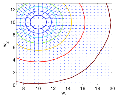
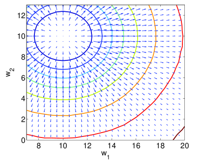
Figure 1: Contours and gradients plots of the performance surfaces: (a) C-Loss; (b) KRSL

III APPLICATION TO ADAPTIVE FILTERING

III-A Performance Surface

Consider the identification of an FIR system:

d(i)=W0TX(i)+v(i)𝑑𝑖superscriptsubscript𝑊0𝑇𝑋𝑖𝑣𝑖d(i)=W_{0}^{T}X(i)+v(i) (22)

where d(i)𝑑𝑖d(i)\in\mathbb{R} denotes an observed response at time i𝑖i ,W0msubscript𝑊0superscript𝑚{W_{0}}\in\mathbb{R}^{m} is an unknown weight vector to be estimated, X(i)=[x(im+1),,x(i)]T𝑋𝑖superscript𝑥𝑖𝑚1𝑥𝑖𝑇X(i)={\left[{x(i-m+1),\cdots,x(i)}\right]^{T}} is the input vector (known value), and v(i)𝑣𝑖v(i) stands for an additive noise (usually independent of the input). Let Wm𝑊superscript𝑚{W}\in\mathbb{R}^{m} be the estimated value of the weight vector. Then the KRSL cost (as a function of W𝑊W is also referred to as the performance surface) is

JKRSL(W)subscript𝐽𝐾𝑅𝑆𝐿𝑊\displaystyle{J_{KRSL}}(W) =1Nλi=1Nexp(λ(1κσ(e(i))))absent1𝑁𝜆superscriptsubscript𝑖1𝑁𝜆1subscript𝜅𝜎𝑒𝑖\displaystyle=\frac{1}{{N\lambda}}\sum\limits_{i=1}^{N}{\exp\left({\lambda\left({1-{\kappa_{\sigma}}\left({e(i)}\right)}\right)}\right)} (23)
=1Nλi=1Nexp(λ(1κσ(d(i)WTX(i))))absent1𝑁𝜆superscriptsubscript𝑖1𝑁𝜆1subscript𝜅𝜎𝑑𝑖superscript𝑊𝑇𝑋𝑖\displaystyle{\rm{}}=\frac{1}{{N\lambda}}\sum\limits_{i=1}^{N}{\exp\left({\lambda\left({1-{\kappa_{\sigma}}\left({d(i)-{W^{T}}X(i)}\right)}\right)}\right)}

with e(i)=d(i)WTX(i)𝑒𝑖𝑑𝑖superscript𝑊𝑇𝑋𝑖e(i)=d(i)-{W^{T}}X(i) being the error at time i𝑖i and N𝑁N the number of samples. The optimal solution can be solved by minimizing the cost function JKRSL(W)subscript𝐽𝐾𝑅𝑆𝐿𝑊{J_{KRSL}}(W). This optimization principle is called in this paper the minimum kernel risk-sensitive loss (MKRSL) criterion. The following theorem holds.

Theorem 1 (Optimal Solution): The optimal solution under the MKRSL criterion satisfies

WMKRSL=[i=1Nh(e(i))X(i)X(i)T]1[i=1Nh(e(i))d(i)X(i)]subscript𝑊𝑀𝐾𝑅𝑆𝐿superscriptdelimited-[]superscriptsubscript𝑖1𝑁𝑒𝑖𝑋𝑖𝑋superscript𝑖𝑇1delimited-[]superscriptsubscript𝑖1𝑁𝑒𝑖𝑑𝑖𝑋𝑖{W_{MKRSL}}\!\!=\!\!\!{\left[{\sum\limits_{i=1}^{N}{h\left({e(i)}\right)}X(i)X{{(i)}^{T}}}\!\!\right]^{-1}}\!\!\left[{\sum\limits_{i=1}^{N}{h\left({e(i)}\right)}d(i)X(i)}\right] (24)

where
h(e(i))=exp(λ(1κσ(d(i)WTX(i))))κσ(d(i)WTX(i))𝑒𝑖𝜆1subscript𝜅𝜎𝑑𝑖superscript𝑊𝑇𝑋𝑖subscript𝜅𝜎𝑑𝑖superscript𝑊𝑇𝑋𝑖h(e(i))\!\!=\!\!\exp\!\left(\!{\lambda\!\left(\!{1\!-\!{\kappa_{\sigma}}\left({d(i)\!\!-\!{W^{T}}X(i)}\right)}\right)}\right){\kappa_{\sigma}}\!\left(\!{d(i)\!\!-\!{W^{T}}X(i)}\!\right), provided that the matrix i=1Nh(e(i))X(i)X(i)Tsuperscriptsubscript𝑖1𝑁𝑒𝑖𝑋𝑖𝑋superscript𝑖𝑇\sum\limits_{i=1}^{N}{h\left(\!{e(i)}\!\right)\!}X(i)X{(i)^{T}} is invertible.

Proof: It is easy to derive

WJKRSL(W)=0𝑊subscript𝐽𝐾𝑅𝑆𝐿𝑊0\displaystyle\frac{\partial}{{\partial W}}{J_{KRSL}}(W)=0 (25)
i=1Nexp(λ(1κσ(d(i)WTX(i))))×\displaystyle\Rightarrow\sum\limits_{i=1}^{N}{\exp\left({\lambda\left({1-{\kappa_{\sigma}}\left({d(i)-{W^{T}}X(i)}\right)}\right)}\right)}\times
κσ(d(i)WTX(i))(d(i)WTX(i))X(i)=0subscript𝜅𝜎𝑑𝑖superscript𝑊𝑇𝑋𝑖𝑑𝑖superscript𝑊𝑇𝑋𝑖𝑋𝑖0\displaystyle{\kappa_{\sigma}}\left({d(i)-{W^{T}}X(i)}\right)\left({d(i)-{W^{T}}X(i)}\right)X(i)=0
[i=1Nh(e(i))X(i)X(i)T]W=[i=1Nh(e(i))d(i)X(i)]absentdelimited-[]superscriptsubscript𝑖1𝑁𝑒𝑖𝑋𝑖𝑋superscript𝑖𝑇𝑊delimited-[]superscriptsubscript𝑖1𝑁𝑒𝑖𝑑𝑖𝑋𝑖\displaystyle\Rightarrow\left[{\sum\limits_{i=1}^{N}{h\left({e(i)}\right)}X(i)X{{(i)}^{T}}}\right]W=\left[{\sum\limits_{i=1}^{N}{h\left({e(i)}\right)}d(i)X(i)}\right]
WMKRSL=[i=1Nh(e(i))X(i)X(i)T]1×\displaystyle\Rightarrow{W_{MKRSL}}={\left[{\sum\limits_{i=1}^{N}{h\left({e(i)}\right)}X(i)X{{(i)}^{T}}}\right]^{-1}}\times
[i=1Nh(e(i))d(i)X(i)]delimited-[]superscriptsubscript𝑖1𝑁𝑒𝑖𝑑𝑖𝑋𝑖\displaystyle\;\;\;\;\;\;\;\;\;\;\;\;\;\;\;\;\;\;\;\;\;\;\;\;\;\left[{\sum\limits_{i=1}^{N}{h\left({e(i)}\right)}d(i)X(i)}\right]

Remark 4: We have h(e(i))1𝑒𝑖1h(e(i))\to 1 as σ𝜎\sigma\to\infty. In this case, the optimal solution WMKRSLsubscript𝑊𝑀𝐾𝑅𝑆𝐿{W_{MKRSL}} will be equal to the well-known Wiener solution. In addition, it is worth noting that the equation (24) does not provide a closed-form solution because the right hand side of (24) depends on W𝑊W through the error e(i)𝑒𝑖e(i) .

Now we compare the performance surfaces of the proposed KRSL and C-Loss. For the case m=2𝑚2m=2 (for visualization purpose), the contours and gradients (with respect to W𝑊W) of the performance surfaces are plotted in Fig.1, where W0=[10,10]Tsubscript𝑊0superscript1010𝑇{W_{0}}={\left[{10,10}\right]^{T}} , σ=2.0𝜎2.0\sigma=2.0 , λ=10𝜆10\lambda=10 , N=10000𝑁10000N=10000 , and the input {x(i)}𝑥𝑖\left\{{x(i)}\right\} and noise {v(i)}𝑣𝑖\left\{{v(i)}\right\} are both zero-mean white Gaussian processes with unit variance. From Fig.1, one can see that the performance surface of the C-Loss is very flat (where the gradients are very small) when the estimated value is far away from the optimal solution (i.e. W0subscript𝑊0{W_{0}} ), whereas it becomes very sharp near the optimal solution. For a gradient-based search algorithm, such a performance surface may lead to slow convergence speed especially when the initial estimate is far away from the optimal solution and possibly low accuracy at final stage due to misadjustments caused by large gradients near the optimal solution. By contrast, the performance surface of the KRSL has three regions: i) when the estimated value is close to the optimum, the gradients will become small to reduce the misadjustments; ii) when the estimated value is away from the optimum, the gradients will become large to speed up the convergence; iii) when the estimated value is further away from the optimum, the gradients will decrease gradually to zero to avoid big fluctuations possibly caused by large outliers. Therefore, compared with the C-Loss, the KRSL can offer potentially a more efficient solution, enabling simultaneously faster convergence and higher accuracy while maintaining the robustness to outliers.

ξ=1c(2σ2log(11λlog[exp(λ(1exp(εv22σ2)))+NMM(exp(λ)1)])+εv)𝜉1𝑐2superscript𝜎211𝜆𝜆1superscriptsubscript𝜀𝑣22superscript𝜎2𝑁𝑀𝑀𝜆1subscript𝜀𝑣\xi=\frac{1}{c}\left({\sqrt{-2{\sigma^{2}}\log\left({1-\frac{1}{\lambda}\log\left[{\exp\left({\lambda\left({1-\exp\left({-\frac{{\varepsilon_{v}^{2}}}{{2{\sigma^{2}}}}}\right)}\right)}\right)+\frac{{N-M}}{M}\left({\exp(\lambda)-1}\right)}\right]}\right)}+{\varepsilon_{v}}}\right) (26)
ρ=1c(βlog(11λlog[exp(λ(1(11λlog[exp(λ)NMM(exp(λ)1)])1/β2))+NMM(exp(λ)1)])log{11λlog[exp(λ)NMM(exp(λ)1)]}+1)𝜌1𝑐𝛽11𝜆𝜆1superscript11𝜆𝜆𝑁𝑀𝑀𝜆11/superscript𝛽2𝑁𝑀𝑀𝜆111𝜆𝜆𝑁𝑀𝑀𝜆11\rho=\frac{1}{c}\left({\beta\sqrt{\frac{{\log\left({1-\frac{1}{\lambda}\log\left[{\exp\left({\lambda\left({1-{{\left({1-\frac{1}{\lambda}\log\left[{\exp(\lambda)-\frac{{N-M}}{M}\left({\exp(\lambda)-1}\right)}\right]}\right)}^{{1\mathord{\left/{\vphantom{1{{\beta^{2}}}}}\right.\kern-1.2pt}{{\beta^{2}}}}}}}\right)}\right)+\frac{{N-M}}{M}\left({\exp(\lambda)-1}\right)}\right]}\right)}}{{\log\left\{{1-\frac{1}{\lambda}\log\left[{\exp(\lambda)-\frac{{N-M}}{M}\left({\exp(\lambda)-1}\right)}\right]}\right\}}}}+1}\right) (27)

III-B Robustness Analysis

Similar to the MCC criterion, the MKRSL criterion is also robust to impulsive noises (or large outliers). In the following, we present some theoretical results on the robustness of the MKRSL criterion. For mathematical tractability, we consider only the scalar FIR identification case ( m=1𝑚1m=1 ). In this case, the weight W𝑊W and input X(i)𝑋𝑖X(i) are both scalars.

First, we give some notations. Let εv>0subscript𝜀𝑣0{\varepsilon_{v}}>0 be a positive number, IN={1,2,,N}subscript𝐼𝑁12𝑁{I_{N}}=\left\{{1,2,\cdots,N}\right\} be the sample index set, and I(εv)={i:iIN,|v(i)|εv}𝐼subscript𝜀𝑣conditional-set𝑖formulae-sequence𝑖subscript𝐼𝑁𝑣𝑖subscript𝜀𝑣I\left({{\varepsilon_{v}}}\right)=\left\{{i:i\in{I_{N}},\left|{v(i)}\right|\leq{\varepsilon_{v}}}\right\} be a subset of INsubscript𝐼𝑁{I_{N}} satisfying iI(εv)for-all𝑖𝐼subscript𝜀𝑣\forall i\in I\left({{\varepsilon_{v}}}\right) , |v(i)|εv𝑣𝑖subscript𝜀𝑣\left|{v(i)}\right|\leq{\varepsilon_{v}} . In addition, the following two assumptions are made:

Assumption 1: N>|I(εv)|=M>N2𝑁𝐼subscript𝜀𝑣𝑀𝑁2N>\left|{I\left({{\varepsilon_{v}}}\right)}\right|=M>\frac{N}{2}, where |I(εv)|𝐼subscript𝜀𝑣\left|{I\left({{\varepsilon_{v}}}\right)}\right| denotes the cardinality of the set I(εv)𝐼subscript𝜀𝑣I\left({{\varepsilon_{v}}}\right) ;

Assumption 2: c>0𝑐0\exists c>0 such that iI(εv)for-all𝑖𝐼subscript𝜀𝑣\forall i\in I\left({{\varepsilon_{v}}}\right) , |X(i)|c𝑋𝑖𝑐\left|{X(i)}\right|\geq c.

Remark 5: The Assumption 1 means that there are M𝑀M ( more than N2𝑁2\frac{N}{2}) samples in which the amplitudes of the additive noises satisfy |v(i)|εv𝑣𝑖subscript𝜀𝑣\left|{v(i)}\right|\leq{\varepsilon_{v}}, and NM𝑁𝑀N-M (at least one) samples that may contain large outliers with |v(i)|>εv𝑣𝑖subscript𝜀𝑣\left|{v(i)}\right|>{\varepsilon_{v}} (possibly |v(i)|εvmuch-greater-than𝑣𝑖subscript𝜀𝑣\left|{v(i)}\right|\gg{\varepsilon_{v}}). The Assumption 2 is reasonable since for a finite number of samples, the minimum amplitude is non-zero in general.

With the above notations and assumptions, the following theorem holds:

Theorem 2: if σ>εv2log{11λlog[exp(λ)NMM(exp(λ)1)]}𝜎subscript𝜀𝑣211𝜆𝜆𝑁𝑀𝑀𝜆1\sigma>\frac{{{\varepsilon_{v}}}}{{\sqrt{-2\log\left\{{1-\frac{1}{\lambda}\log\left[{\exp(\lambda)-\frac{{N-M}}{M}\left({\exp(\lambda)-1}\right)}\right]}\right\}}}}, then the optimal solution WMKRSLsubscript𝑊𝑀𝐾𝑅𝑆𝐿{W_{MKRSL}} under the MKRSL criterion satisfies |WMKRSLW0|ξsubscript𝑊𝑀𝐾𝑅𝑆𝐿subscript𝑊0𝜉\left|{{W_{MKRSL}}-{W_{0}}}\right|\leq\xi, where the expression of ξ𝜉\xi is shown at the the bottom of the page.

Proof: See Appendix.

The​ following​ corollary​ is​ a​ direct​ consequence​ of​ Theorem​ 2:

Corollary 1: If
σ>εv2log{11λlog[exp(λ)NMM(exp(λ)1)]}𝜎subscript𝜀𝑣211𝜆𝜆𝑁𝑀𝑀𝜆1\sigma>\frac{{{\varepsilon_{v}}}}{{\sqrt{-2\log\left\{{1-\frac{1}{\lambda}\log\left[{\exp(\lambda)-\frac{{N-M}}{M}\left({\exp(\lambda)-1}\right)}\right]}\right\}}}}, then the optimal solution WMKRSLsubscript𝑊𝑀𝐾𝑅𝑆𝐿{W_{MKRSL}} under MKRSL satisfies |WMKRSLW0|ρεvsubscript𝑊𝑀𝐾𝑅𝑆𝐿subscript𝑊0𝜌subscript𝜀𝑣\left|{{W_{MKRSL}}-{W_{0}}}\right|\leq\rho{\varepsilon_{v}}, where the expression of the constant ρ𝜌\rho is shown at the the bottom of the page, with β=σεv2log{11λlog[exp(λ)NMM(exp(λ)1)]}𝛽𝜎subscript𝜀𝑣211𝜆𝜆𝑁𝑀𝑀𝜆1\beta=\frac{\sigma}{{{\varepsilon_{v}}}}\sqrt{-2\log\left\{{1-\frac{1}{\lambda}\log\left[{\exp(\lambda)-\frac{{N-M}}{M}\left({\exp(\lambda)-1}\right)}\right]}\right\}}.

Remark 5: According to Corollary 1, if the kernel bandwidth σ𝜎\sigma is larger than a certain value, the absolute value of the estimation error εMKRSL=WMKRSLW0subscript𝜀𝑀𝐾𝑅𝑆𝐿subscript𝑊𝑀𝐾𝑅𝑆𝐿subscript𝑊0{\varepsilon_{MKRSL}}={W_{MKRSL}}-{W_{0}} will be upper bounded by ρεv𝜌subscript𝜀𝑣\rho{\varepsilon_{v}}. If εvsubscript𝜀𝑣{\varepsilon_{v}} is very small, the upper bound ρεv𝜌subscript𝜀𝑣\rho{\varepsilon_{v}} will also be very small, which implies that the MKRSL solution WMKRSLsubscript𝑊𝑀𝐾𝑅𝑆𝐿{W_{MKRSL}} can be very close to the true value (W0subscript𝑊0{W_{0}}) even in presence of (NM)𝑁𝑀(N-M) outliers (whose values can be arbitrarily large), provided that there are M𝑀M(M>N/2𝑀𝑁/2M>{N\mathord{\left/{\vphantom{N2}}\right.\kern-1.2pt}2}) samples disturbed by small noises (bounded by εvsubscript𝜀𝑣{\varepsilon_{v}}).

For the vector case (m>1𝑚1m>1), it is very difficult to derive an upper bound on the norm of the estimation error. However, we believe that the above results for scalar case explain clearly why and how the MKRSL criterion will be robust to large outliers.

III-C Stochastic Gradient Adaptive Algorithm

Stochastic gradient based adaptive algorithms have been widely used in many practical applications, especially those involving online adaptation. Under the MKRSL criterion, the instantaneous cost function at time i𝑖i is

J^KRSL=1λexp(λ(1κσ(e(i))))subscript^𝐽𝐾𝑅𝑆𝐿1𝜆𝜆1subscript𝜅𝜎𝑒𝑖{\hat{J}_{KRSL}}=\frac{1}{\lambda}\exp\left({\lambda\left({1-{\kappa_{\sigma}}\left({e(i)}\right)}\right)}\right) (28)

Then a stochastic gradient based adaptive filtering algorithm can be easily derived as

W(i+1)=W(i)μW(i)J^KRSL𝑊𝑖1𝑊𝑖𝜇𝑊𝑖subscript^𝐽𝐾𝑅𝑆𝐿\displaystyle W(i+1)=W(i)-\mu\frac{\partial}{{\partial W(i)}}{{\hat{J}}_{KRSL}} (29)
=W(i)+μσ2exp(λ(1κσ(e(i))))κσ(e(i))e(i)X(i)absent𝑊𝑖𝜇superscript𝜎2𝜆1subscript𝜅𝜎𝑒𝑖subscript𝜅𝜎𝑒𝑖𝑒𝑖𝑋𝑖\displaystyle{\rm{}}=W(i)+\frac{\mu}{{{\sigma^{2}}}}\exp\left({\lambda\left({1-{\kappa_{\sigma}}(e(i))}\right)}\right){\kappa_{\sigma}}(e(i))e(i)X(i)
=W(i)+ηexp(λ(1κσ(e(i))))κσ(e(i))e(i)X(i)absent𝑊𝑖𝜂𝜆1subscript𝜅𝜎𝑒𝑖subscript𝜅𝜎𝑒𝑖𝑒𝑖𝑋𝑖\displaystyle{\rm{}}=W(i)+\eta\exp\left({\lambda\left({1-{\kappa_{\sigma}}(e(i))}\right)}\right){\kappa_{\sigma}}(e(i))e(i)X(i)

where W(i)𝑊𝑖W(i) denotes the estimated weight vector at time i𝑖i, and η=μσ2𝜂𝜇superscript𝜎2\eta=\frac{\mu}{{{\sigma^{2}}}} is the step-size parameter. We call the above algorithm the MKRSL algorithm. In this work, we use the same abbreviation for an optimization criterion and the corresponding algorithm when no confusion can arise from the context.

The MKRSL algorithm (29) can also be expressed as

W(i+1)=W(i)+η(i)e(i)X(i)𝑊𝑖1𝑊𝑖𝜂𝑖𝑒𝑖𝑋𝑖W(i+1)=W(i)+\eta(i)e(i)X(i) (30)

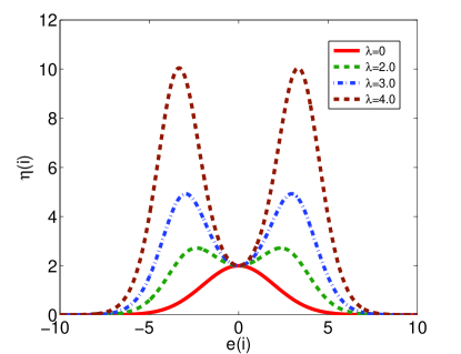
which is a least mean square (LMS) algorithm with a variable step-size (VSS) η(i)=ηexp(λ(1κσ(e(i))))κσ(e(i))𝜂𝑖𝜂𝜆1subscript𝜅𝜎𝑒𝑖subscript𝜅𝜎𝑒𝑖\eta(i)=\eta\exp\left({\lambda\left({1-{\kappa_{\sigma}}(e(i))}\right)}\right){\kappa_{\sigma}}(e(i)) .

We have the following observations:

1) As λ0+𝜆limit-from0\lambda\to 0+, we have η(i)ηκσ(e(i))𝜂𝑖𝜂subscript𝜅𝜎𝑒𝑖\eta(i)\to\eta{\kappa_{\sigma}}(e(i)). In this case, the MKRSL algorithm becomes the MCC algorithm [21, 22]:

W(i+1)=W(i)+ηκσ(e(i))e(i)X(i)𝑊𝑖1𝑊𝑖𝜂subscript𝜅𝜎𝑒𝑖𝑒𝑖𝑋𝑖W(i+1)=W(i)+\eta{\kappa_{\sigma}}(e(i))e(i)X(i) (31)

2) As σ𝜎\sigma\to\infty, we have η(i)η𝜂𝑖𝜂\eta(i)\to\eta. In this case, the MKRSL algorithm will reduce to the original LMS algorithm (with a fixed step-size):

W(i)=W(i1)+ηe(i)X(i)𝑊𝑖𝑊𝑖1𝜂𝑒𝑖𝑋𝑖W(i)=W(i-1)+\eta e(i)X(i) (32)

Fig. 2 shows the curves of η(i)𝜂𝑖\eta(i) as a function of e(i)𝑒𝑖e(i) for different values of λ𝜆\lambda (where σ=η=2.0𝜎𝜂2.0\sigma=\eta=2.0). As one can see, when λ=0𝜆0\lambda=0 (corresponding to the MCC algorithm), the step-size η(i)𝜂𝑖\eta(i) will reach the maximum at the origin (e(i)=0𝑒𝑖0e(i)=0).When λ>0𝜆0\lambda>0, however, the step-size η(i)𝜂𝑖\eta(i) may reach the maximum at a location away from the origin, potentially leading to faster convergence speed and better accuracy. For any λ𝜆\lambda, the step-size η(i)𝜂𝑖\eta(i) will approach zero as |e(i)|𝑒𝑖\left|{e(i)}\right|\to\infty , which implies that the MKRSL algorithm will be insensitive (or robust) to large errors.

Note that the computational complexity of the MKRSL algorithm is almost the same as the MCC algorithm. The only extra computational demand is to calculate the term exp(λ(1κσ(e(i))))𝜆1subscript𝜅𝜎𝑒𝑖\exp\left({\lambda\left({1-{\kappa_{\sigma}}(e(i))}\right)}\right).

Refer to caption
Figure 2: Curves of η(i)𝜂𝑖\eta(i) as a function of e(i)𝑒𝑖e(i) (σ=η=2.0𝜎𝜂2.0\sigma=\eta=2.0 )

III-D Mean Square Convergence Performance

The mean square convergence behavior is very important for an adaptive filtering algorithm. There have been extensive studies on the mean square convergence of various adaptive filtering algorithms in the literature [35]. The proposed MKRSL algorithm belongs to a general class of adaptive filtering algorithms [36, 37]:

W(i+1)=W(i)+ηf(e(i))X(i)𝑊𝑖1𝑊𝑖𝜂𝑓𝑒𝑖𝑋𝑖W(i+1)=W(i)+\eta f\left({e(i)}\right)X(i) (33)

where f(e(i))𝑓𝑒𝑖f\left({e(i)}\right) is a nonlinear function of e(i)=d(i)WT(i)X(i)𝑒𝑖𝑑𝑖superscript𝑊𝑇𝑖𝑋𝑖e(i)=d(i)-{W^{T}}(i)X(i) , which, for the MKRSL algorithm, is

f(e(i))=exp(λ(1κσ(e(i))))κσ(e(i))e(i)𝑓𝑒𝑖𝜆1subscript𝜅𝜎𝑒𝑖subscript𝜅𝜎𝑒𝑖𝑒𝑖f\left({e(i)}\right)=\exp\left({\lambda\left({1-{\kappa_{\sigma}}(e(i))}\right)}\right){\kappa_{\sigma}}(e(i))e(i) (34)

For the case d(i)=W0TX(i)+v(i)𝑑𝑖superscriptsubscript𝑊0𝑇𝑋𝑖𝑣𝑖d(i)={W_{0}}^{T}X(i)+v(i), the following relation holds [36]:

E[W~(i+1)2]=Edelimited-[]superscriptnorm~𝑊𝑖12absent\displaystyle\textbf{E}\left[{{{\left\|{\tilde{W}(i+1)}\right\|}^{2}}}\right]= E[W~(i)2]2ηE[ea(i)f(e(i))]Edelimited-[]superscriptnorm~𝑊𝑖22𝜂Edelimited-[]subscript𝑒𝑎𝑖𝑓𝑒𝑖\displaystyle\textbf{E}\left[{{{\left\|{\tilde{W}(i)}\right\|}^{2}}}\right]-2\eta\textbf{E}\left[{{e_{a}}(i)f(e(i))}\right] (35)
+η2E[X(i)2f2(e(i))]superscript𝜂2Edelimited-[]superscriptnorm𝑋𝑖2superscript𝑓2𝑒𝑖\displaystyle+{\eta^{2}}\textbf{E}\left[{{{\left\|{X(i)}\right\|}^{2}}{f^{2}}(e(i))}\right]

where W~(i)=W0W(i)~𝑊𝑖subscript𝑊0𝑊𝑖\tilde{W}(i)={W_{0}}-W(i) is the weigh error vector at iteration i𝑖i, and ea(i)=W~T(i)X(i)subscript𝑒𝑎𝑖superscript~𝑊𝑇𝑖𝑋𝑖{e_{a}}(i)={\tilde{W}^{T}}(i)X(i) is the a priori error. The relation (35) is a direct consequence of the energy conservation relation[36, 37].
1) Transient Behavior

Based on (35) and under some assumptions, one can derive a dynamic equation to characterize the transient behavior of the weight error power E[W~(i)2]Edelimited-[]superscriptnorm~𝑊𝑖2\textbf{E}\left[{{{\left\|{\tilde{W}(i)}\right\|}^{2}}}\right]. Specifically, the following theorem holds [37].

Theorem 3: Consider the adaptive filtering algorithm (33), where e(i)=d(i)WT(i)X(i)𝑒𝑖𝑑𝑖superscript𝑊𝑇𝑖𝑋𝑖e(i)=d(i)-{W^{T}}(i)X(i), and d(i)=W0TX(i)+v(i)𝑑𝑖superscriptsubscript𝑊0𝑇𝑋𝑖𝑣𝑖d(i)={W_{0}}^{T}X(i)+v(i). Assume that the noise process {v(i)}𝑣𝑖\left\{{v(i)}\right\} is i.i.d. and independent of the zero-mean input X(i)𝑋𝑖X(i) and that the filter is long enough so that ea(i)subscript𝑒𝑎𝑖{e_{a}}(i) is zero-mean Gaussian and that X(i)2superscriptnorm𝑋𝑖2{\left\|{X(i)}\right\|^{2}} and f2(e(i))superscript𝑓2𝑒𝑖{f^{2}}\left({e(i)}\right) are uncorrelated. Then it holds that

E[W~(i+1)Σ2]=E[W~(i)Σ2]Edelimited-[]superscriptsubscriptnorm~𝑊𝑖1Σ2Edelimited-[]superscriptsubscriptnorm~𝑊𝑖Σ2\displaystyle\textbf{E}\left[{\left\|{\tilde{W}(i+1)}\right\|_{\Sigma}^{2}}\right]=\textbf{E}\left[{\left\|{\tilde{W}(i)}\right\|_{\Sigma}^{2}}\right] (36)
2ηhG(E[W~(i)X(i)XT(i)2])×E[W~(i)ΣX(i)XT(i)2]2𝜂subscript𝐺Edelimited-[]superscriptsubscriptnorm~𝑊𝑖𝑋𝑖superscript𝑋𝑇𝑖2Edelimited-[]superscriptsubscriptnorm~𝑊𝑖Σ𝑋𝑖superscript𝑋𝑇𝑖2\displaystyle-2\eta{h_{G}}\left({\textbf{E}\left[{\left\|{\tilde{W}(i)}\right\|_{X(i){X^{T}}(i)}^{2}}\right]}\right)\times\textbf{E}\left[{\left\|{\tilde{W}(i)}\right\|_{\Sigma X(i){X^{T}}(i)}^{2}}\right]
+η2E[X(i)Σ2]hU(E[W~(i)X(i)XT(i)2])superscript𝜂2Edelimited-[]superscriptsubscriptnorm𝑋𝑖Σ2subscript𝑈Edelimited-[]superscriptsubscriptnorm~𝑊𝑖𝑋𝑖superscript𝑋𝑇𝑖2\displaystyle{\rm{}}+{\eta^{2}}\textbf{E}\left[{\left\|{X(i)}\right\|_{\Sigma}^{2}}\right]{h_{U}}\left({\textbf{E}\left[{\left\|{\tilde{W}(i)}\right\|_{X(i){X^{T}}(i)}^{2}}\right]}\right)

where W~(i)Σ2=W~T(i)ΣW~(i)superscriptsubscriptnorm~𝑊𝑖Σ2superscript~𝑊𝑇𝑖Σ~𝑊𝑖\left\|{\tilde{W}(i)}\right\|_{\Sigma}^{2}={\tilde{W}^{T}}(i)\Sigma\tilde{W}(i), and the functions hG(.){h_{G}}(.) and hU(.){h_{U}}(.) are defined by

hG(E[ea2(i)])=E[ea(i)f(e(i))]E[ea2(i)]subscript𝐺Edelimited-[]superscriptsubscript𝑒𝑎2𝑖Edelimited-[]subscript𝑒𝑎𝑖𝑓𝑒𝑖Edelimited-[]superscriptsubscript𝑒𝑎2𝑖\displaystyle{h_{G}}\left({\textbf{E}\left[{e_{a}^{2}(i)}\right]}\right)=\frac{{\textbf{E}\left[{{e_{a}}(i)f(e(i))}\right]}}{{\textbf{E}\left[{e_{a}^{2}(i)}\right]}} (37)
hU(E[ea2(i)])=E[f2(e(i))]subscript𝑈Edelimited-[]superscriptsubscript𝑒𝑎2𝑖Edelimited-[]superscript𝑓2𝑒𝑖\displaystyle{h_{U}}\left({\textbf{E}\left[{e_{a}^{2}(i)}\right]}\right)=\textbf{E}\left[{{f^{2}}(e(i))}\right]

Proof: A detailed derivation can be found in [37].

For the MKRSL algorithm, x>0for-all𝑥0\forall x>0,the functions hG(x)subscript𝐺𝑥{h_{G}}(x) and hU(x)subscript𝑈𝑥{h_{U}}(x) can be expressed as

hG(x)=subscript𝐺𝑥absent\displaystyle{h_{G}}(x)= 12πx3yexp(λ(1κσ(y+v)))×\displaystyle\frac{1}{{\sqrt{2\pi{x^{3}}}}}\int_{-\infty}^{\infty}{\int_{-\infty}^{\infty}{y\exp\left({\lambda\left({1-{\kappa_{\sigma}}(y+v)}\right)}\right)}}\times (38)
κσ(y+v)(y+v)exp(y22x)pv(v)dydvsubscript𝜅𝜎𝑦𝑣𝑦𝑣superscript𝑦22𝑥subscript𝑝𝑣𝑣𝑑𝑦𝑑𝑣\displaystyle{\kappa_{\sigma}}(y+v)(y+v)\exp\left({-\frac{{{y^{2}}}}{{2x}}}\right){p_{v}}(v)dydv
hU(x)=subscript𝑈𝑥absent\displaystyle{h_{U}}(x)= 12πxexp(2λ(1κσ(y+v)))×\displaystyle\frac{1}{{\sqrt{2\pi x}}}\int_{-\infty}^{\infty}{\int_{-\infty}^{\infty}{\exp\left({2\lambda\left({1-{\kappa_{\sigma}}(y+v)}\right)}\right)}}\times
κσ/2(y+v)(y+v)2exp(y22x)pv(v)dydvsubscript𝜅𝜎/2𝑦𝑣superscript𝑦𝑣2superscript𝑦22𝑥subscript𝑝𝑣𝑣𝑑𝑦𝑑𝑣\displaystyle{\kappa_{{\sigma\mathord{\left/{\vphantom{\sigma{\sqrt{2}}}}\right.\kern-1.2pt}{\sqrt{2}}}}}(y+v){(y+v)^{2}}\exp\left({-\frac{{{y^{2}}}}{{2x}}}\right){p_{v}}(v)dydv

where pv(.){p_{v}}(.) denotes the PDF of the noise v(i)𝑣𝑖v(i). In general, there are no closed-form expressions for hG(.){h_{G}}(.) and hU(.){h_{U}}(.) . But the two functions can still be calculated by numerical integration.

Remark 6: Using (36), one can construct the convergence curves of the weight error power. For example, if, in addition, the input sequence {X(i)}𝑋𝑖\left\{{X(i)}\right\} is i.i.d., with covariance matrix R=σx2IRsuperscriptsubscript𝜎𝑥2I\textbf{R}=\sigma_{x}^{2}\textbf{I}, where I denotes the identity matrix, we have

E[W~(i+1)2]=E[W~(i)2]Edelimited-[]superscriptnorm~𝑊𝑖12Edelimited-[]superscriptnorm~𝑊𝑖2\displaystyle\textbf{E}\left[{{{\left\|{\tilde{W}(i+1)}\right\|}^{2}}}\right]=\textbf{E}\left[{{{\left\|{\tilde{W}(i)}\right\|}^{2}}}\right] (39)
2ησx2hG(σx2E[W~(i)2])×E[W~(i)2]2𝜂superscriptsubscript𝜎𝑥2subscript𝐺superscriptsubscript𝜎𝑥2Edelimited-[]superscriptnorm~𝑊𝑖2Edelimited-[]superscriptnorm~𝑊𝑖2\displaystyle-2\eta\sigma_{x}^{2}{h_{G}}\left({\sigma_{x}^{2}\textbf{E}\left[{{{\left\|{\tilde{W}(i)}\right\|}^{2}}}\right]}\right)\times\textbf{E}\left[{{{\left\|{\tilde{W}(i)}\right\|}^{2}}}\right]
+η2σx2mhU(σx2E[W~(i)2])superscript𝜂2superscriptsubscript𝜎𝑥2𝑚subscript𝑈superscriptsubscript𝜎𝑥2Edelimited-[]superscriptnorm~𝑊𝑖2\displaystyle{\rm{}}+{\eta^{2}}\sigma_{x}^{2}m{h_{U}}\left({\sigma_{x}^{2}\textbf{E}\left[{{{\left\|{\tilde{W}(i)}\right\|}^{2}}}\right]}\right)

which is a recursion equation for generating the convergence curves of E[W~(i)2]Edelimited-[]superscriptnorm~𝑊𝑖2\textbf{E}\left[{{{\left\|{\tilde{W}(i)}\right\|}^{2}}}\right].
2) Steady-State Performance

Let S=limiE[ea2(i)]𝑆subscript𝑖Edelimited-[]superscriptsubscript𝑒𝑎2𝑖S=\mathop{\lim}\limits_{i\to\infty}\textbf{E}\left[{e_{a}^{2}(i)}\right] be the steady-state excess mean square error (EMSE). According to [37], with the same setting of Theorem 3, the EMSE will be a positive solution of the following equation:

S=η2Tr(R)hU(S)hG(S)𝑆𝜂2𝑇𝑟Rsubscript𝑈𝑆subscript𝐺𝑆S=\frac{\eta}{2}Tr\left(\textbf{R}\right)\frac{{{h_{U}}(S)}}{{{h_{G}}(S)}} (40)

Since the functions hG(x)subscript𝐺𝑥{h_{G}}(x) and hU(x)subscript𝑈𝑥{h_{U}}(x) have no closed-form expressions in general, it is very difficult to solve the above equation. However, one can use a Taylor expansion method to obtain an approximate value of S𝑆S. In this way, the following theorem holds.

Theorem 4: Consider the adaptive filtering algorithm (33), where e(i)=d(i)WT(i)X(i)𝑒𝑖𝑑𝑖superscript𝑊𝑇𝑖𝑋𝑖e(i)=d(i)-{W^{T}}(i)X(i), and d(i)=W0TX(i)+v(i)𝑑𝑖superscriptsubscript𝑊0𝑇𝑋𝑖𝑣𝑖d(i)={W_{0}}^{T}X(i)+v(i). Assume that the noise process {v(i)}𝑣𝑖\left\{{v(i)}\right\} is zero-mean, i.i.d. and independent of the input X(i)𝑋𝑖X(i) and that the a priori error ea(i)subscript𝑒𝑎𝑖{e_{a}}(i) is zero-mean and independent of the noise v(i)𝑣𝑖v(i) and that ea(i)subscript𝑒𝑎𝑖{e_{a}}(i) is relatively small at steady-state such that its third and higher-order terms are negligible. Then we have

SηTr(R)E[f2(v)]2E[f(v)]ηTr(R)E[f(v)f′′(v)+|f(v)|2]𝑆𝜂𝑇𝑟REdelimited-[]superscript𝑓2𝑣2Edelimited-[]superscript𝑓𝑣𝜂𝑇𝑟REdelimited-[]𝑓𝑣superscript𝑓′′𝑣superscriptsuperscript𝑓𝑣2S\approx\frac{{\eta Tr(\textbf{R})\textbf{E}\left[{{f^{2}}(v)}\right]}}{{2\textbf{E}\left[{f^{\prime}(v)}\right]-\eta Tr(\textbf{R})\textbf{E}\left[{f(v)f^{\prime\prime}(v)+{{\left|{f^{\prime}(v)}\right|}^{2}}}\right]}} (41)

where f(v)superscript𝑓𝑣f^{\prime}(v) and f′′(v)superscript𝑓′′𝑣f^{\prime\prime}(v) are the first and second derivatives of f(v)𝑓𝑣f(v).

Proof: see [24]. for a detailed derivation.

For the MKRSL algorithm, the derivatives f(v)superscript𝑓𝑣f^{\prime}(v) and f′′(v)superscript𝑓′′𝑣f^{\prime\prime}(v) are respectively

f(v)=exp(λ(1κσ(v)))κσ(v)(1+λv2σ2κσ(v)v2σ2)superscript𝑓𝑣𝑒𝑥𝑝𝜆1subscript𝜅𝜎𝑣subscript𝜅𝜎𝑣1𝜆superscript𝑣2superscript𝜎2subscript𝜅𝜎𝑣superscript𝑣2superscript𝜎2f^{\prime}(v)=exp(\lambda(1-{\kappa_{\sigma}}(v))){\kappa_{\sigma}}(v)\left({1+\lambda\frac{{{v^{2}}}}{{{\sigma^{2}}}}{\kappa_{\sigma}}(v)-\frac{{{v^{2}}}}{{{\sigma^{2}}}}}\right) (42)
f′′(v)=exp(λ(1κσ(v)))κσ(v)×\displaystyle f^{\prime\prime}(v)=exp(\lambda(1-{\kappa_{\sigma}}(v))){\kappa_{\sigma}}(v)\times (43)
(λ2v3σ4κσ/2(v)+3λσ2v3λv3σ4κσ(v)+v33vσ2σ4)superscript𝜆2superscript𝑣3superscript𝜎4subscript𝜅𝜎/2𝑣3𝜆superscript𝜎2𝑣3𝜆superscript𝑣3superscript𝜎4subscript𝜅𝜎𝑣superscript𝑣33𝑣superscript𝜎2superscript𝜎4\displaystyle\!\left({\frac{{{\lambda^{2}}{v^{3}}}}{{{\sigma^{4}}}}{\kappa_{{\sigma\mathord{\left/{\vphantom{\sigma 2}}\right.\kern-1.2pt}2}}}(v)\!+\!\frac{{3\lambda{\sigma^{2}}v\!-\!3\lambda{v^{3}}}}{{{\sigma^{4}}}}{\kappa_{\sigma}}(v)\!+\!\frac{{{v^{3}}\!-\!3v{\sigma^{2}}}}{{{\sigma^{4}}}}}\right)

Remark 7: Given a noise PDF pv(.){p_{v}}(.), one can calculate the expectations E[f2(v)]Edelimited-[]superscript𝑓2𝑣\textbf{E}\left[{{f^{2}}(v)}\right] , E[f(v)]Edelimited-[]superscript𝑓𝑣\textbf{E}\left[{f^{\prime}(v)}\right] and E[f(v)f′′(v)+|f(v)|2]Edelimited-[]𝑓𝑣superscript𝑓′′𝑣superscriptsuperscript𝑓𝑣2\textbf{E}\left[{f(v)f^{\prime\prime}(v)+{{\left|{f^{\prime}(v)}\right|}^{2}}}\right] , usually by numerical integration, and then obtain an approximate value of S𝑆S by using (41).

IV SIMULATION RESULTS

In this section, simulation results are presented to confirm the theoretical analysis and demonstrate the performance of the proposed MKRSL algorithm.

IV-A Verification of Theoretical Results

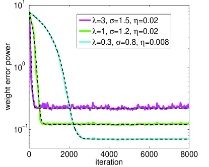
First, we demonstrate the theoretical and simulated convergence curves (in terms of the weight error power) of the MKRSL algorithm with different parameter settings. In the simulation, the filter length is set at m=20𝑚20m=20, and the initial weight vector is a null vector. The input and noise are both zero-mean white Gaussian processes with unit variance. The theoretical convergence curves and simulated ones averaged over 1000 Monte Carlo runs are shown in Fig. 3. As one can see, the theoretical curves match very well with those obtained by simulations.
Refer to caption
Figure 3: Theoretical (black dashed) and simulated (solid) convergence curves with different parameter settings

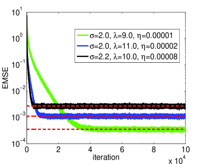
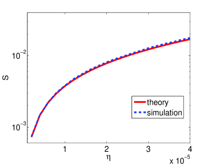
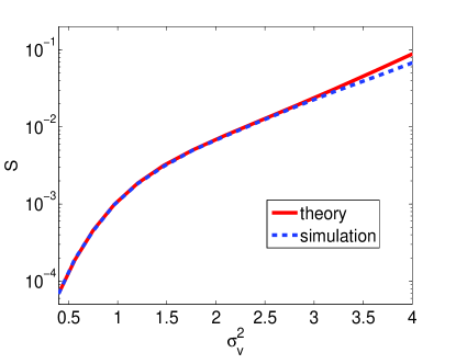
We also illustrate the steady-state EMSEs. The unknown system and input are the same as in the previous simulation. The theoretical steady-state EMSEs calculated by (41) and simulated convergence curves (over 500 Monte Carlo runs) with different parameter settings are shown in Fig. 4, where the noise is assumed to be zero-mean Uniform distributed with unit variance. We can see that after transient stages the simulated curves will converge almost exactly toward the theoretical values. In addition, the theoretical and simulated steady-state EMSEs with different step-sizes and noise variances are shown in Fig. 5. To obtain the simulated steady-state EMSEs, we perform100 Monte Carlo simulations, and in each simulation, 200000 iterations are run to ensure the algorithm to achieve the steady-state, and the steady-state EMSEs are obtained as the averages over the last 10000 iterations. Again, simulation results agree very well with the theoretical predictions. To further confirm the theoretical results, we present in Table II the theoretical and simulated steady-state EMSEs for different noise distributions, where Gaussian and Laplace noises are both zero-mean with unit variance, Binary noise is either -1.0 or 1.0 (each with probability 0.5), and Cauchy noise is distributed with PDF p(v)=1/[π(1+v2)]𝑝𝑣1delimited-[]𝜋1superscript𝑣2p(v)=1/[\pi(1+{v^{2}})].

Refer to caption
Figure 4: Theoretical steady-state EMSEs (red dashed) and simulated convergence curves with different parameter settings.
Refer to caption
Refer to caption
Figure 5: Theoretical and simulated steady-state EMSEs: (a) with different step-sizes ( λ=8.0𝜆8.0\lambda=8.0, σ=1.0𝜎1.0\sigma=1.0, σv2=1.0superscriptsubscript𝜎𝑣21.0\sigma_{v}^{2}=1.0); (b) with different noise variances ( λ=8.0𝜆8.0\lambda=8.0, σ=1.0𝜎1.0\sigma=1.0, η=0.000003𝜂0.000003\eta={\rm{0}}{\rm{.000003}}).
TABLE II: Theoretical and simulated steady-state EMSEs for different noise distributions
Noise distribution Parameter setting Theory Simulation
Gaussian λ=8.0,σ=1.0,η=0.000003formulae-sequence𝜆8.0formulae-sequence𝜎1.0𝜂0.000003\lambda=8.0,\;\sigma=1.0,\;\eta={\rm{0}}{\rm{.000003}} 0.0030 0.0031±0.0005plus-or-minus0.00310.00050.0031\pm 0.0005
Binary λ=9.0,σ=1.0,η=0.000003formulae-sequence𝜆9.0formulae-sequence𝜎1.0𝜂0.000003\lambda=9.0,\;\sigma=1.0,\;\eta={\rm{0}}{\rm{.000003}} 0.000116 0.000117±0.000018plus-or-minus0.0001170.0000180.000117\pm 0.000018
Laplace λ=9.0,σ=1.0,η=0.000002formulae-sequence𝜆9.0formulae-sequence𝜎1.0𝜂0.000002\lambda=9.0,\;\sigma=1.0,\;\eta={\rm{0}}{\rm{.000002}} 0.0065 0.0064±0.0012plus-or-minus0.00640.00120.0064\pm 0.0012
Cauuchy λ=8.0,σ=1.0,η=0.000002formulae-sequence𝜆8.0formulae-sequence𝜎1.0𝜂0.000002\lambda=8.0,\;\sigma=1.0,\;\eta={\rm{0}}{\rm{.000002}} 0.0049 0.0049±0.0013plus-or-minus0.00490.00130.0049\pm 0.0013

IV-B Performance Comparison with Other Algorithms

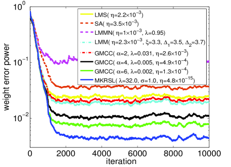
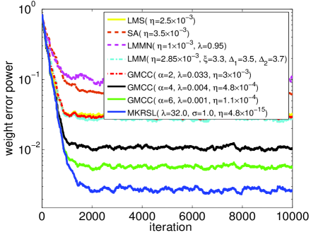
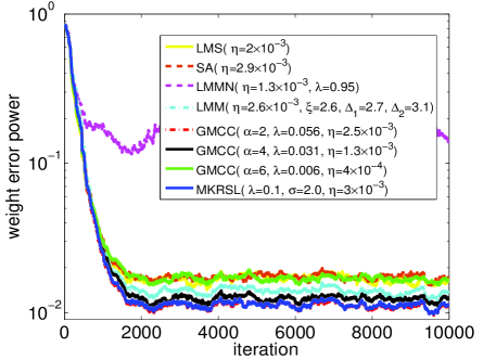
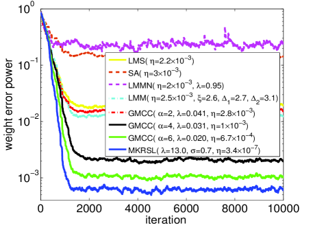
Next, we compare the performance of the MKRSL with that of the LMS, sign algorithm (SA) [38, 39], least mean mixed-norm (LMMN) algorithm [40], least mean M-estimate (LMM) algorithm [41] and GMCC (α=2,4,6𝛼246\alpha=2,4,6)[17]. The weight vector of the unknown system is assumed to be W0=[0.1,0.2,0.3,0.4,0.5,0.4,0.3,0.2,0.1]Tsubscript𝑊0superscript0.10.20.30.40.50.40.30.20.1𝑇{W_{0}}={\left[{0.1,0.2,0.3,0.4,0.5,0.4,0.3,0.2,0.1}\right]^{T}}, and the initial weight vector of the adaptive filters is a null vector. The input signal is zero-mean Gaussian with variance 1.0 and the noise is assumed to be v(i)=(1a(i))A(i)+a(i)B(i)𝑣𝑖1𝑎𝑖𝐴𝑖𝑎𝑖𝐵𝑖v(i)=(1-a(i))A(i)+a(i)B(i) , where a(i)𝑎𝑖a(i) is a binary i.i.d. process with Pr{a(i)=1}=cPr𝑎𝑖1𝑐\Pr\left\{{a(i)=1}\right\}=c and Pr{a(i)=0}=1cPr𝑎𝑖01𝑐\Pr\left\{{a(i)=0}\right\}=1-c (0c10𝑐10\leq c\leq 1 ), and A(i)𝐴𝑖A(i) andB(i)𝐵𝑖B(i) are two mutually independent noise processes (both independent of a(i)𝑎𝑖a(i)) with variances σA2\sigma{}_{A}^{2} and σB2superscriptsubscript𝜎𝐵2\sigma_{B}^{2}. Usually the variance σB2superscriptsubscript𝜎𝐵2\sigma_{B}^{2} is much larger than the variance σA2\sigma{}_{A}^{2}, thus B(i)𝐵𝑖B(i) can represent large outliers. Without mentioned otherwise, c𝑐c is set to 0.06 and B(i)𝐵𝑖B(i) is a white Gaussian process with σB2=15superscriptsubscript𝜎𝐵215\sigma_{B}^{2}{\rm{=}}15. For the noise A(i)𝐴𝑖A(i), we consider four cases: a) zero-mean Gaussian distribution with σ=A21.0\sigma{}_{A}^{2}{\rm{=}}1.0; b) Binary distribution with Pr{A(i)=1}=Pr{A(i)=1}=0.5𝑃𝑟𝐴𝑖1𝑃𝑟𝐴𝑖10.5Pr\{A(i)=-1\}=Pr\{A(i)=1\}=0.5; c) Uniform distribution over [5,5]55[-\sqrt{5},\sqrt{5}]; and d) Sine wave noise 2sin(ω)2𝜔2\sin(\omega), with ω𝜔\omega uniform distributed over [0,2π]02𝜋[0,2\pi]. Fig. 6 shows the convergence curves (in terms of the weight error power) averaged over 100 independent Monte Carlo runs. In the simulation, the step-sizes are chosen such that all the algorithms have almost the same initial convergence speed, and other parameters (if any) for each algorithm are experimentally selected to achieve desirable performance. The selected values of these parameters are included in the figures. It can be seen clearly that the MKRSL algorithm can significantly outperform other algorithms.
Refer to caption
Refer to caption
Refer to caption
Refer to caption
Figure 6: Convergence curves with different distributions of A(i)𝐴𝑖A(i): (a) Gaussian; (b) Binary; (c) Uniform; (d) Sine wave

IV-C Effects of the Parameters λ𝜆\lambda and σ𝜎\sigma

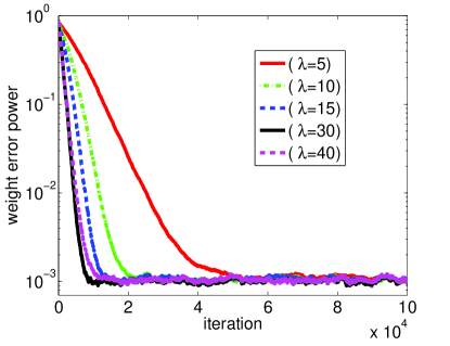
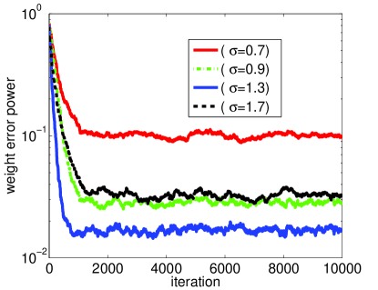
Further, we show how the performance of the MKRSL will be influenced by the risk-sensitive parameter λ𝜆\lambda and kernel bandwidth σ𝜎\sigma. With the same noise as in Fig.6 (c), the convergence curves of the MKRSL with different λ𝜆\lambda and σ𝜎\sigma are illustrated in Fig. 7. For each convergence curve, the step-size is chosen to achieve almost the same steady-state performance (Fig.7 (a)) or initial convergence speed (Fig.7 (b)). One can observe that both parameters have significant influence on the convergence behavior and desirable performance can be obtained only with appropriate parameter setting. How to determine an optimal value of λ𝜆\lambda or σ𝜎\sigma is however very involved and is left open in this work. In a practical application, the parameters λ𝜆\lambda and σ𝜎\sigma can be set manually or determined by trial and error methods.

IV-D Effects of the Outliers

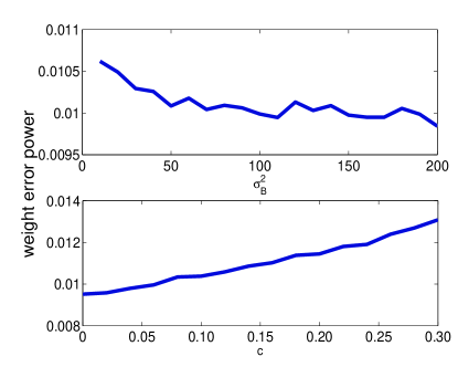
Finally, we demonstrate the robust performance of the MKRSL with different outlier variances ( σB2superscriptsubscript𝜎𝐵2\sigma_{B}^{2}) and occurrence frequencies ( c𝑐c).With the same noise model as in Fig.6 (a), the steady-state weight error powers with different σB2superscriptsubscript𝜎𝐵2\sigma_{B}^{2} and c𝑐c are plotted in Fig.8. From the simulation results we can observe: i) the MKRSL is very robust with respect to the amplitudes of outliers and its performance can even become better with the variance σB2superscriptsubscript𝜎𝐵2\sigma_{B}^{2} increasing; ii) the algorithm is also robust with respect to the occurrence frequencies of outliers, and with c𝑐c increasing from 0% to 30%, the steady-state weight error power will increase very slightly (just from 0.0096 to 0.013).
Refer to caption
Refer to caption
Figure 7: Convergence curves of MKRSL: (a) with different λ𝜆\lambda ( σ=1.0𝜎1.0\sigma=1.0); (b) with different σ𝜎\sigma ( λ=10𝜆10\lambda=10)
Refer to caption
Figure 8: Steady-state weight error powers with different outlier variances and occurrence frequencies

V CONCLUSION

As a nonlinear similarity measure in kernel space, correntropy has been successfully applied in non-Gaussian signal processing and machine learning. To further improve the performance surface, we propose in this work a new similarity measure in kernel space, called the kernel risk-sensitive loss (KRSL), which takes the same form as that of the traditional risk-sensitive loss, but defined in different spaces. Compared with correntropy, the KRSL can offer a more efficient performance surface that enables a gradient based method to achieve faster convergence speed and higher accuracy while still maintaining the robustness to outliers. Some important properties of the KRSL were presented. We applied the KRSL to adaptive filtering and investigated the robustness. Particularly, a robust adaptive filtering algorithm, namely the MKRSL algorithm, was derived and its mean square convergence performance was analyzed. Simulation results have confirmed the theoretical predictions and demonstrated that the new algorithm can achieve better convergence performance when compared with some existing algorithms.

Appendix A PROOF OF THEOREM 2

Proof: Since WMKRSL=argminWJKRSL(W)subscript𝑊𝑀𝐾𝑅𝑆𝐿subscript𝑊subscript𝐽𝐾𝑅𝑆𝐿𝑊{W_{MKRSL}}=\arg\mathop{\min}\limits_{W}{J_{KRSL}}(W) , we have JKRSL(WMKRSL)JKRSL(W0)subscript𝐽𝐾𝑅𝑆𝐿subscript𝑊𝑀𝐾𝑅𝑆𝐿subscript𝐽𝐾𝑅𝑆𝐿subscript𝑊0{J_{KRSL}}({W_{MKRSL}})\leq{J_{KRSL}}({W_{0}}) . To prove |WMKRSLW0|ξsubscript𝑊𝑀𝐾𝑅𝑆𝐿subscript𝑊0𝜉\left|{{W_{MKRSL}}-{W_{0}}}\right|\leq\xi, it will suffice to prove JKRSL(W)>JKRSL(Wo)subscript𝐽𝐾𝑅𝑆𝐿𝑊subscript𝐽𝐾𝑅𝑆𝐿subscript𝑊𝑜{J_{KRSL}}(W)>{J_{KRSL}}({W_{o}}) for any W𝑊W satisfying |WW0|>ξ𝑊subscript𝑊0𝜉\left|{W-{W_{0}}}\right|>\xi. Since N>M>N2𝑁𝑀𝑁2N>M>\frac{N}{2}, we have 0<NMM<10𝑁𝑀𝑀10<\frac{{N-M}}{M}<1, and 0<11λlog[exp(λ)NMM(exp(λ)1)]<1011𝜆𝜆𝑁𝑀𝑀𝜆110<1-\frac{1}{\lambda}\log\left[{\exp(\lambda)-\frac{{N-M}}{M}\left({\exp(\lambda)-1}\right)}\right]<1. As σ>εv2log{11λlog[exp(λ)NMM(exp(λ)1)]}𝜎subscript𝜀𝑣211𝜆𝜆𝑁𝑀𝑀𝜆1\sigma>\frac{{{\varepsilon_{v}}}}{{\sqrt{-2\log\left\{{1-\frac{1}{\lambda}\log\left[{\exp(\lambda)-\frac{{N-M}}{M}\left({\exp(\lambda)-1}\right)}\right]}\right\}}}}, it follows easily that

0<1λlog[exp(λ(1exp(εv22σ2)))+NMM(exp(λ)1)]<101𝜆𝜆1superscriptsubscript𝜀𝑣22superscript𝜎2𝑁𝑀𝑀𝜆110\!<\!\frac{1}{\lambda}\!\log\!\!\left[{\exp\!\left(\!{\lambda\!\left(\!{1\!-\!\exp\!\left(\!{\!-\!\frac{{\varepsilon_{v}^{2}}}{{2{\sigma^{2}}}}}\!\right)}\!\right)}\!\right)\!+\!\frac{{N\!-\!\!M}}{M}\!\left({\exp\!(\lambda)\!-\!1}\!\right)}\!\right]\!\!<\!1 (44)

Further, if

|WW0|>ξ=1c𝑊subscript𝑊0𝜉1𝑐\displaystyle\left|{W-{W_{0}}}\right|>\xi=\frac{1}{c} (45)
(2σ2log(11λlog[exp(λ(1exp(εv22σ2)))+NMM(exp(λ)1)])+εv)2superscript𝜎211𝜆𝜆1superscriptsubscript𝜀𝑣22superscript𝜎2𝑁𝑀𝑀𝜆1subscript𝜀𝑣\displaystyle\!\!\!\!\!\left(\!\!\!{\sqrt{\!\!-\!2\!{\sigma^{2}}\!\log\!\!\left(\!\!{1\!\!\!-\!\!\frac{1}{\lambda}\!\log\!\!\left[\!{\exp\!\!\left({\!\!\lambda\!\left(\!\!{1\!\!\!-\!\!\exp\!\!\left(\!{\!-\!\frac{{\varepsilon_{v}^{2}}}{{2{\sigma^{2}}}}}\!\!\right)}\!\!\right)}\!\!\right)\!\!\!+\!\!\frac{{N\!\!\!-\!\!\!M}}{M}\!\!\left({\!\exp\!(\!\lambda\!)\!\!-\!1}\!\right)}\!\right]}\!\right)}\!\!\!+\!\!\!{\varepsilon_{v}}}\!\!\!\right)

we have iI(εv)for-all𝑖𝐼subscript𝜀𝑣\forall i\in I\left({{\varepsilon_{v}}}\right),

|e(i)|=|(W0W)X(i)+v(i)|𝑒𝑖subscript𝑊0𝑊𝑋𝑖𝑣𝑖\displaystyle\left|{e(i)}\right|=\left|{\left({{W_{0}}-W}\right)X(i)+v(i)}\right| (46)
|W0W|×|X(i)||v(i)|absentsubscript𝑊0𝑊𝑋𝑖𝑣𝑖\displaystyle{\rm{}}\geq\left|{{W_{0}}-W}\right|\times\left|{X(i)}\right|-\left|{v(i)}\right|
>(a)ξcεv=superscript𝑎𝜉𝑐subscript𝜀𝑣absent\displaystyle{\rm{}}\mathop{>}\limits^{(a)}\xi c-{\varepsilon_{v}}=
2σ2log(11λlog[exp(λ(1exp(εv22σ2)))+NMM(exp(λ)1)])2superscript𝜎211𝜆𝜆1superscriptsubscript𝜀𝑣22superscript𝜎2𝑁𝑀𝑀𝜆1\displaystyle\!\!\!\!\!\!\sqrt{\!-\!2{\sigma^{2}}\!\log\!\!\left(\!\!{1\!-\!\frac{1}{\lambda}\!\log\!\!\!\left[\!{\exp\!\!\left(\!\!{\lambda\!\!\left(\!\!{1\!\!-\!\exp\!\!\left({\!\!-\!\frac{{\varepsilon_{v}^{2}}}{{2{\sigma^{2}}}}}\!\!\right)}\!\!\right)}\!\!\right)\!\!+\!\frac{{N\!\!-\!M}}{M}\!\left({\exp\!(\lambda\!)\!-\!1}\!\right)}\!\right]}\!\right)}

where (a) comes from the Assumption 2 and |WW0|>ξ𝑊subscript𝑊0𝜉\left|{W-{W_{0}}}\right|>\xi and |v(i)|εv𝑣𝑖subscript𝜀𝑣\left|{v(i)}\right|\leq{\varepsilon_{v}}. Thus iI(εv)for-all𝑖𝐼subscript𝜀𝑣\forall i\in I\left({{\varepsilon_{v}}}\right),

exp(λ(1exp(e2(i)2σ2)))exp(λ)>𝜆1superscript𝑒2𝑖2superscript𝜎2𝜆absent\displaystyle\exp\left({\lambda\left({1-\exp\left({-\frac{{{e^{2}}(i)}}{{2{\sigma^{2}}}}}\right)}\right)}\right)-\exp(\lambda)> (47)
exp(λ(1exp(εv22σ2)))exp(λ)NMM(1exp(λ))𝜆1superscriptsubscript𝜀𝑣22superscript𝜎2𝜆𝑁𝑀𝑀1𝜆\displaystyle\exp\left({\lambda\left({1-\exp\left({-\frac{{\varepsilon_{v}^{2}}}{{2{\sigma^{2}}}}}\right)}\right)}\right)-\exp(\lambda)-\frac{{N-M}}{M}\left({1-\exp(\lambda)}\right)

Then we have JKRSL(W)>JKRSL(Wo)subscript𝐽𝐾𝑅𝑆𝐿𝑊subscript𝐽𝐾𝑅𝑆𝐿subscript𝑊𝑜{J_{KRSL}}(W)>{J_{KRSL}}({W_{o}}) for any W𝑊W satisfying |WW0|>ξ𝑊subscript𝑊0𝜉\left|{W-{W_{0}}}\right|>\xi, because

JKRSL(W)1λexp(λ)subscript𝐽𝐾𝑅𝑆𝐿𝑊1𝜆𝜆\displaystyle{J_{KRSL}}(W)-\frac{1}{\lambda}\exp(\lambda) (48)
=1Nλi=1N{exp(λ(1exp(e2(i)2σ2)))exp(λ)}absent1𝑁𝜆superscriptsubscript𝑖1𝑁𝜆1superscript𝑒2𝑖2superscript𝜎2𝜆\displaystyle=\frac{1}{{N\lambda}}\sum\limits_{i=1}^{N}{\left\{{\exp\left({\lambda\left({1-\exp\left({-\frac{{{e^{2}}(i)}}{{2{\sigma^{2}}}}}\right)}\right)}\right)-\exp(\lambda)}\right\}}
>1NλiI(εv){exp(λ(1exp(εv22σ2)))exp(λ)NMM(1exp(λ))}absent1𝑁𝜆subscript𝑖𝐼subscript𝜀𝑣𝜆1superscriptsubscript𝜀𝑣22superscript𝜎2𝜆𝑁𝑀𝑀1𝜆\displaystyle>\!\!\frac{1}{{N\lambda}}\!\!\sum\limits_{i\in I\left({{\varepsilon_{v}}}\right)}\!\!\!\!{\!\left\{{\!\!\exp\!\!\left({\!\!\lambda\!\!\left(\!\!{1\!\!-\!\exp\!\!\left({\!\!-\!\frac{{\varepsilon_{v}^{2}}}{{2{\sigma^{2}}}}}\!\!\right)}\!\!\right)}\!\!\right)\!\!-\!\!\exp\!(\!\lambda)\!\!-\!\frac{{N\!\!-\!\!M}}{M}\!\left({1\!\!-\!\exp\!(\lambda\!)}\!\right)}\!\!\right\}}
+1NλiI(εv){exp(λ(1exp(e2(i)2σ2)))exp(λ)}1𝑁𝜆subscript𝑖𝐼subscript𝜀𝑣𝜆1superscript𝑒2𝑖2superscript𝜎2𝜆\displaystyle+\frac{1}{{N\lambda}}\sum\limits_{i\notin I\left({{\varepsilon_{v}}}\right)}{\left\{{\exp\left({\lambda\left({1-\exp\left({-\frac{{{e^{2}}(i)}}{{2{\sigma^{2}}}}}\right)}\right)}\right)-\exp(\lambda)}\right\}}
>(b)1NλiI(εv){exp(λ(1exp(εv22σ2)))exp(λ)NMM(1exp(λ))}superscript𝑏1𝑁𝜆subscript𝑖𝐼subscript𝜀𝑣𝜆1superscriptsubscript𝜀𝑣22superscript𝜎2𝜆𝑁𝑀𝑀1𝜆\displaystyle\mathop{>}\limits^{(b)}\!\!\frac{1}{{N\lambda}}\!\!\!\!\sum\limits_{i\in I\left({{\varepsilon_{v}}}\right)}\!\!\!\!{\left\{{\!\exp\!\!\left({\!\!\lambda\!\!\left(\!{1\!\!-\!\exp\!\!\left(\!{\!-\!\frac{{\varepsilon_{v}^{2}}}{{2{\sigma^{2}}}}}\!\!\right)}\!\!\right)}\!\!\right)\!\!-\!\exp\!(\!\lambda\!)\!\!-\!\frac{{N\!\!-\!\!M}}{M}\!\!\left({1\!\!-\!\exp(\!\lambda\!)}\!\right)}\!\!\right\}}
+1Nλ(NM)(1exp(λ))1𝑁𝜆𝑁𝑀1𝜆\displaystyle+\frac{1}{{N\lambda}}\left({N-M}\right)\left({1-\exp(\lambda)}\right)
=1NλiI(εv){exp(λ(1exp(εv22σ2)))exp(λ)}absent1𝑁𝜆subscript𝑖𝐼subscript𝜀𝑣𝜆1superscriptsubscript𝜀𝑣22superscript𝜎2𝜆\displaystyle=\frac{1}{{N\lambda}}\sum\limits_{i\in I\left({{\varepsilon_{v}}}\right)}{\left\{{\exp\left({\lambda\left({1-\exp\left({-\frac{{\varepsilon_{v}^{2}}}{{2{\sigma^{2}}}}}\right)}\right)}\right)-\exp(\lambda)}\right\}}
(c)1NλiI(εv){exp(λ(1exp(v2(i)2σ2)))exp(λ)}superscript𝑐1𝑁𝜆subscript𝑖𝐼subscript𝜀𝑣𝜆1superscript𝑣2𝑖2superscript𝜎2𝜆\displaystyle\mathop{\geq}\limits^{(c)}\frac{1}{{N\lambda}}\sum\limits_{i\in I\left({{\varepsilon_{v}}}\right)}{\left\{{\exp\left({\lambda\left({1-\exp\left({-\frac{{{v^{2}}(i)}}{{2{\sigma^{2}}}}}\right)}\right)}\right)-\exp(\lambda)}\right\}}
>(d)1Nλi=1N{exp(λ(1exp(v2(i)2σ2)))exp(λ)}superscript𝑑1𝑁𝜆superscriptsubscript𝑖1𝑁𝜆1superscript𝑣2𝑖2superscript𝜎2𝜆\displaystyle\mathop{>}\limits^{(d)}\frac{1}{{N\lambda}}\sum\limits_{i=1}^{N}{\left\{{\exp\left({\lambda\left({1-\exp\left({-\frac{{{v^{2}}(i)}}{{2{\sigma^{2}}}}}\right)}\right)}\right)-\exp(\lambda)}\right\}}
=JKRSL(W0)1λexp(λ)absentsubscript𝐽𝐾𝑅𝑆𝐿subscript𝑊01𝜆𝜆\displaystyle={J_{KRSL}}({W_{0}})-\frac{1}{\lambda}\exp(\lambda)

where (b) comes from exp(λ(1exp(e2(i)2σ2)))1𝜆1superscript𝑒2𝑖2superscript𝜎21\exp\left({\lambda\left({1-\exp\left({-\frac{{{e^{2}}(i)}}{{2{\sigma^{2}}}}}\right)}\right)}\right)\geq 1, (c) follows from εv|v(i)|subscript𝜀𝑣𝑣𝑖{\varepsilon_{v}}\geq\left|{v(i)}\right|, iI(εv)for-all𝑖𝐼subscript𝜀𝑣\forall i\in I\left({{\varepsilon_{v}}}\right), and (d) is due to exp(λ(1exp(v2(i)2σ2)))exp(λ)<0𝜆1superscript𝑣2𝑖2superscript𝜎2𝜆0\exp\left({\lambda\left({1-\exp\left({-\frac{{{v^{2}}(i)}}{{2{\sigma^{2}}}}}\right)}\right)}\right)-\exp(\lambda)<0. This completes the proof.

References

  • [1] Jose C Principe. Information theoretic learning: Renyi’s entropy and kernel perspectives. Springer Science & Business Media, 2010.
  • [2] Badong Chen, Yu Zhu, Jinchun Hu, and Jose C Principe. System parameter identification: information criteria and algorithms. Newnes, 2013.
  • [3] David Jacobson. Optimal stochastic linear systems with exponential performance criteria and their relation to deterministic differential games. IEEE Transactions on Automatic control, 18(2):124–131, 1973.
  • [4] Mathew R James, John S Baras, and Robert J Elliott. Risk-sensitive control and dynamic games for partially observed discrete-time nonlinear systems. IEEE transactions on automatic control, 39(4):780–792, 1994.
  • [5] Yungang Liu, Zigang Pan, and Songjiao Shi. Output feedback control design for strict-feedback stochastic nonlinear systems under a risk-sensitive cost. IEEE Transactions on Automatic Control, 48(3):509–513, 2003.
  • [6] Rene K Boel, Matthew R James, and Ian R Petersen. Robustness and risk-sensitive filtering. IEEE Transactions on Automatic Control, 47(3):451–461, 2002.
  • [7] James T Lo and Thomas Wanner. Existence and uniqueness of risk-sensitive estimates. IEEE transactions on automatic control, 47(11):1945–1948, 2002.
  • [8] Deniz Erdogmus and Jose C Principe. From linear adaptive filtering to nonlinear information processing-the design and analysis of information processing systems. IEEE Signal Processing Magazine, 23(6):14–33, 2006.
  • [9] Erhan Gokcay and Jose C. Principe. Information theoretic clustering. IEEE Transactions on Pattern Analysis and Machine Intelligence, 24(2):158–171, 2002.
  • [10] Deniz Erdogmus and Jose C Principe. An error-entropy minimization algorithm for supervised training of nonlinear adaptive systems. IEEE Transactions on Signal Processing, 50(7):1780–1786, 2002.
  • [11] Deniz Erdogmus and Jose C Principe. Generalized information potential criterion for adaptive system training. IEEE Transactions on Neural Networks, 13(5):1035–1044, 2002.
  • [12] Ignacio Santamaría, Deniz Erdogmus, and Jose C Principe. Entropy minimization for supervised digital communications channel equalization. IEEE Transactions on Signal Processing, 50(5):1184–1192, 2002.
  • [13] Badong Chen, Yu Zhu, and Jinchun Hu. Mean-square convergence analysis of adaline training with minimum error entropy criterion. IEEE Transactions on Neural Networks, 21(7):1168–1179, 2010.
  • [14] Badong Chen, Pingping Zhu, and José C Principe. Survival information potential: a new criterion for adaptive system training. IEEE Transactions on Signal Processing, 60(3):1184–1194, 2012.
  • [15] Ignacio Santamaría, Puskal P Pokharel, and José Carlos Principe. Generalized correlation function: definition, properties, and application to blind equalization. IEEE Transactions on Signal Processing, 54(6):2187–2197, 2006.
  • [16] Weifeng Liu, Puskal P Pokharel, and José C Príncipe. Correntropy: properties and applications in non-gaussian signal processing. IEEE Transactions on Signal Processing, 55(11):5286–5298, 2007.
  • [17] Chen Badong, Xing Lei, Zhao Haiquan, Zheng Nanning, and José C Príncipe. Generalized correntropy for robust adaptive filtering. IEEE Transactions on Signal Processing, 64(13):3376–3387, 2016.
  • [18] Ran He, Wei-Shi Zheng, and Bao-Gang Hu. Maximum correntropy criterion for robust face recognition. IEEE Transactions on Pattern Analysis and Machine Intelligence, 33(8):1561–1576, 2011.
  • [19] Ran He, Tieniu Tan, and Liang Wang. Robust recovery of corrupted low-rankmatrix by implicit regularizers. IEEE transactions on pattern analysis and machine intelligence, 36(4):770–783, 2014.
  • [20] Ran He, Bao-Gang Hu, Wei-Shi Zheng, and Xiang-Wei Kong. Robust principal component analysis based on maximum correntropy criterion. IEEE Transactions on Image Processing, 20(6):1485–1494, 2011.
  • [21] Abhishek Singh and Jose C Principe. Using correntropy as a cost function in linear adaptive filters. In 2009 International Joint Conference on Neural Networks, pages 2950–2955. IEEE, 2009.
  • [22] Songlin Zhao, Badong Chen, and Jose C Principe. Kernel adaptive filtering with maximum correntropy criterion. In Neural Networks (IJCNN), The 2011 International Joint Conference on, pages 2012–2017. IEEE, 2011.
  • [23] Abhishek Singh and Jose C Principe. A loss function for classification based on a robust similarity metric. In The 2010 International Joint Conference on Neural Networks (IJCNN), pages 1–6. IEEE, 2010.
  • [24] Badong Chen, Lei Xing, Junli Liang, Nanning Zheng, and Jose C Principe. Steady-state mean-square error analysis for adaptive filtering under the maximum correntropy criterion. IEEE signal processing letters, 21(7):880–884, 2014.
  • [25] Liming Shi and Yun Lin. Convex combination of adaptive filters under the maximum correntropy criterion in impulsive interference. IEEE Signal Processing Letters, 21(11):1385–1388, 2014.
  • [26] Badong Chen, Jianji Wang, Haiquan Zhao, Nanning Zheng, and José C Príncipe. Convergence of a fixed-point algorithm under maximum correntropy criterion. IEEE Signal Processing Letters, 22(10):1723–1727, 2015.
  • [27] Liangjun Chen, Hua Qu, Jihong Zhao, Badong Chen, and Jose C Principe. Efficient and robust deep learning with correntropy-induced loss function. Neural Computing and Applications, 27(4):1019–1031, 2016.
  • [28] Fei Zhu, Abderrahim Halimi, Paul Honeine, Badong Chen, and Nanning Zheng. Correntropy maximization via admm-application to robust hyperspectral unmixing. arXiv preprint arXiv:1602.01729, 2016.
  • [29] Mujahid N Syed, Panos M Pardalos, and Jose C Principe. On the optimization properties of the correntropic loss function in data analysis. Optimization Letters, 8(3):823–839, 2014.
  • [30] Badong Chen and Ren Wang. Risk-sensitive loss in kernel space for robust adaptive filtering. In 2015 IEEE International Conference on Digital Signal Processing (DSP), pages 921–925. IEEE, 2015.
  • [31] Vladimir Naumovich Vapnik and Vlamimir Vapnik. Statistical learning theory, volume 1. Wiley New York, 1998.
  • [32] Bernhard Schölkopf and Alexander J Smola. Learning with kernels: support vector machines, regularization, optimization, and beyond. MIT press, 2002.
  • [33] Johan AK Suykens, Jos De Brabanter, Lukas Lukas, and Joos Vandewalle. Weighted least squares support vector machines: robustness and sparse approximation. Neurocomputing, 48(1):85–105, 2002.
  • [34] Badong Chen and José C Príncipe. Maximum correntropy estimation is a smoothed map estimation. IEEE Signal Processing Letters, 19(8):491–494, 2012.
  • [35] Ali H Sayed. Fundamentals of adaptive filtering. John Wiley & Sons, 2003.
  • [36] Tareq Y Al-Naffouri and Ali H Sayed. Adaptive filters with error nonlinearities: Mean-square analysis and optimum design. EURASIP Journal on Applied Signal Processing, 2001(1):192–205, 2001.
  • [37] Tareq Y Al-Naffouri and Ali H Sayed. Transient analysis of adaptive filters with error nonlinearities. IEEE Transactions on Signal Processing, 51(3):653–663, 2003.
  • [38] Vjohn Mathews and Sung Cho. Improved convergence analysis of stochastic gradient adaptive filters using the sign algorithm. IEEE Transactions on Acoustics, Speech, and Signal Processing, 35(4):450–454, 1987.
  • [39] Min Shao and Chrysostomos L Nikias. Signal processing with fractional lower order moments: stable processes and their applications. Proceedings of the IEEE, 81(7):986–1010, 1993.
  • [40] JA Chambers, O Tanrikulu, and AG Constantinides. Least mean mixed-norm adaptive filtering. Electronics letters, 30(19):1574–1575, 1994.
  • [41] Yuexian Zou, Shing-Chow Chan, and Tung-Sang Ng. Least mean m-estimate algorithms for robust adaptive filtering in impulse noise. IEEE Transactions on Circuits and Systems II: Analog and Digital Signal Processing, 47(12):1564–1569, 2000.