SI-HEP-2016-22
TTP16-031
TTK-16-31
TUM-HEP-1057/16
arXiv:1607.07574 [hep-ph]
October 25, 2016

NNLL soft and Coulomb resummation for squark
and gluino production at the LHC

M. Benekea, J. Piclumb, C. Schwinnc, C. Weverd
aPhysik Department T31, James-Franck-Straße 1, Technische Universität München,
D–85748 Garching, Germany
b Theoretische Physik 1, Naturwissenschaftlich-Technische Fakultät, Universität Siegen, 57068 Siegen, Germany
and
Albert Einstein Center for Fundamental Physics, Institute for Theoretical Physics, University of Bern, 3012 Bern, Switzerland
cInstitut für Theoretische Teilchenphysik und Kosmologie, RWTH Aachen University, D–52056 Aachen, Germany
dInstitute of Nuclear Physics, NCSR ”Demokritos”, GR 15310 Athens, Greece
and
Institute for Theoretical Particle Physics (TTP), Engesserstraße 7, D-76128 Karlsruhe & Institute for Nuclear Physics (IKP), Hermann-von-Helmholtz-Platz 1, D-76344 Eggenstein-Leopoldshafen, Karlsruhe Institute of Technology, Germany

Abstract

We present predictions for the total cross sections for pair production of squarks and gluinos at the LHC including a combined NNLL resummation of soft and Coulomb gluon effects. We derive all terms in the NNLO cross section that are enhanced near the production threshold, which include contributions from spin-dependent potentials and so-called annihilation corrections. The NNLL corrections at s=13𝑠13\sqrt{s}=13 TeV range from up to 20%percent2020\% for squark-squark production to 90%percent9090\% for gluino pair production relative to the NLO results and reduce the theoretical uncertainties of the perturbative calculation to the 10%percent1010\% level. Grid files with our numerical results are publicly available [1].

1 Introduction

Supersymmetry (SUSY) and its realization in the R𝑅R-parity conserving Minimally Supersymmetric Standard Model (MSSM) is a well-studied and motivated extension of the Standard Model (SM) of particle physics. It could provide a solution to shortcomings of the SM such as the absence of a dark matter candidate and it might stabilize the electroweak scale against quantum corrections. The search for SUSY at the TeV scale is therefore a central part of the physics program of the Large Hadron Collider (LHC). The production of squarks q~~𝑞\tilde{q} and gluinos g~~𝑔\tilde{g}, the super-partners of quarks and gluons, through the strong interaction is expected to be an important discovery channel of SUSY, provided these particles are kinematically accessible at the LHC. The most stringent limits from the 7TeV7TeV7~{}\mathrm{TeV} and 8TeV8TeV8~{}\mathrm{TeV} runs of the LHC [2, 3] exclude gluino masses up to mg~=1.3subscript𝑚~𝑔1.3m_{\tilde{g}}=1.3 TeV and superpartners of the quarks of the first two generations below mq~875less-than-or-similar-tosubscript𝑚~𝑞875m_{\tilde{q}}\lesssim 875 GeV. Equal squark and gluino masses can be excluded up to mg~1.7similar-tosubscript𝑚~𝑔1.7m_{\tilde{g}}\sim 1.7 TeV. First results at s=13TeV𝑠13TeV\sqrt{s}=13~{}\mathrm{TeV} raised the mass bounds to mg~1.75less-than-or-similar-tosubscript𝑚~𝑔1.75m_{\tilde{g}}\lesssim 1.75 TeV and mq~1.26less-than-or-similar-tosubscript𝑚~𝑞1.26m_{\tilde{q}}\lesssim 1.26 TeV [4]. However, these bounds depend on assumptions, e.g. on the mass of the lightest supersymmetric particle and on decay chains, and can be evaded, for instance by compressed mass spectra or non-degenerate light-flavour squark masses. The search for SUSY therefore remains a focus of the 131313141414 TeV run of the LHC that has the potential to discover or exclude squarks and gluinos up to the 333 TeV range. Turning exclusion limits on production cross sections into bounds on superparticle masses requires precise predictions for these cross sections, which motivates the computation of higher-order corrections to squark and gluino production. The next-to-leading order (NLO) corrections for production of the light-flavour squarks and gluinos in the supersymmetric extension of quantum chromodynamics (SQCD) have been known for a long time [5] and have been implemented in the program PROSPINO [6]. More recently, additional higher-order QCD corrections have been added to this result in various approximations [7, 8, 9, 10, 11, 12, 13, 14, 15, 16, 17, 18, 19, 20]. Corresponding results for top squarks have been obtained as well [21, 22, 23, 24, 16, 25, 26, 27, 28]. Complementary work to this improvement of total cross sections by higher-order QCD corrections is provided by the computation of electroweak contributions [29, 30, 31, 32, 33, 34, 35, 36], the automation of NLO calculations in the MSSM [37, 38], the matching of NLO corrections to a parton shower [39, 40, 41], the calculation of NLO corrections to squark production and decay [42, 43, 40] and the estimate of finite-width effects [44].

The dominant production channels for squark and gluino production at hadron colliders are pair-production processes of the form

N1N2s~s~X,subscript𝑁1subscript𝑁2~𝑠superscript~𝑠𝑋N_{1}N_{2}\to\tilde{s}\tilde{s}^{\prime}X, (1.1)

where N1,2subscript𝑁12N_{1,2} denote the incoming hadrons and s~~𝑠\tilde{s}, s~superscript~𝑠\tilde{s}^{\prime} the two sparticles. In this paper we will consider all pair-production processes of gluinos and squarks except top squark production. The NLO SQCD corrections to squark and gluino production processes can become very large for heavy sparticle masses [5], up to 100%percent100100\% of the tree-level result for gluino-pair production. This raises the question of the convergence of the perturbative series. A substantial part of the large NLO corrections can be attributed to terms that are enhanced in the limit of a small relative velocity β𝛽\beta of the sparticles,

β=1(ms~+ms~)2s^0,𝛽1superscriptsubscript𝑚~𝑠subscript𝑚superscript~𝑠2^𝑠0\beta=\sqrt{1-\frac{(m_{\tilde{s}}+m_{\tilde{s}^{\prime}})^{2}}{\hat{s}}}\to 0, (1.2)

where s^^𝑠\hat{s} is the partonic centre-of-mass energy. These corrections arise at each order in perturbation theory through threshold logarithms αsln2,1βsubscript𝛼𝑠superscript21𝛽\alpha_{s}\ln^{2,1}\beta due to soft-gluon corrections and through Coulomb corrections of the form αs/βsubscript𝛼𝑠𝛽\alpha_{s}/\beta. The large NLO corrections to squark and gluino production and the significant contribution of the threshold region motivate the resummation of these threshold corrections, i.e.  a reorganization of the perturbation theory under the assumption that both types of threshold corrections are of order one,

αslnβ1,αsβ1.formulae-sequencesimilar-tosubscript𝛼𝑠𝛽1similar-tosubscript𝛼𝑠𝛽1\alpha_{s}\ln\beta\sim 1\,,\quad\frac{\alpha_{s}}{\beta}\sim 1. (1.3)

The accuracy of the resummed perturbative series can be defined by representing the resummed cross section schematically as

σ^pp=subscript^𝜎𝑝superscript𝑝absent\displaystyle\hat{\sigma}_{pp^{\prime}}= σ^pp(0)k=0(αsβ)k(1+αscNNLL+)subscriptsuperscript^𝜎0𝑝superscript𝑝superscriptsubscript𝑘0superscriptsubscript𝛼𝑠𝛽𝑘1subscript𝛼𝑠subscript𝑐NNLL\displaystyle\,\hat{\sigma}^{(0)}_{pp^{\prime}}\,\sum_{k=0}^{\infty}\left(\frac{\alpha_{s}}{\beta}\right)^{\!k}\Bigl{(}1+\alpha_{s}c_{\text{NNLL}}+\ldots\Bigr{)} (1.4)
×exp[lnβg0(αslnβ)(LL)+g1(αslnβ)(NLL)+αsg2(αslnβ)(NNLL)+].absentsubscript𝛽subscript𝑔0subscript𝛼𝑠𝛽(LL)subscriptsubscript𝑔1subscript𝛼𝑠𝛽(NLL)subscriptsubscript𝛼𝑠subscript𝑔2subscript𝛼𝑠𝛽(NNLL)\displaystyle\times\,\exp\Big{[}\underbrace{\ln\beta\,g_{0}(\alpha_{s}\ln\beta)}_{\mbox{(LL)}}+\underbrace{g_{1}(\alpha_{s}\ln\beta)}_{\mbox{(NLL)}}+\underbrace{\alpha_{s}g_{2}(\alpha_{s}\ln\beta)}_{\mbox{(NNLL)}}+\ldots\Big{]}\,.

Methods for the separate resummation of the two towers of corrections are well established and have been applied to squark and gluino production. The resummation of threshold logarithms [45, 46, 47, 48] with a fixed-order treatment of Coulomb corrections was performed at NLL [7, 8, 11, 23] and more recently at NNLL accuracy [15, 18, 26, 20]. The application of Coulomb-resummation [49] to squark and gluino production with a fixed-order treatment of threshold logarithms was considered in [8, 10, 14, 13].

In these approaches, only one of the two variables in (1.3) is considered to be of order one in the threshold region, which is not justified a priori. Therefore a combined resummation of soft and Coulomb corrections is desirable and was established in [50, 12] using effective-theory methods. The application of this method to squark and gluino production at NLL accuracy [16] has revealed a significant effect of Coulomb corrections and soft-Coulomb interference effects that can be as large as the soft corrections alone. Since the joint soft and Coulomb corrections at NLL can show an enhancement of up to 100%percent100100\% relative to the NLO cross section for some processes and large sparticle masses [16], a combined NNLL treatment seems to be required for a stabilisation of the perturbative behaviour. We note that when the Coulomb corrections are not summed, some of the sizeable corrections at NLL in the combined soft-Coulomb resummation appear only at the next order (NNLL) in pure soft-gluon resummation. Ref. [20] indeed confirms the earlier finding of a significant soft-Coulomb interference effect. In the present paper we perform for the first time such a combined soft and Coulomb resummation for squark and gluino production at NNLL accuracy. Preliminary results have been presented already in [19]. A combination of Coulomb corrections and NNLL soft resummation has also been performed for the case of top-squark bound states (“stoponium”) in [27] using a formalism similar to ours.

With respect to our previous work on NNLL resummation for top quark production [51, 52], this paper contains several new theoretical results and features: We derive the extension of the spin-dependent non-Coulomb αs2lnβsuperscriptsubscript𝛼𝑠2𝛽\alpha_{s}^{2}\ln\beta terms given for top-pair production in [53] to squark and gluino production (these results have been quoted already in [19]). We also generalize the additional logarithm found in [54] for top-pair production to squark and gluino production and show how it arises in the effective-theory framework. For the soft-gluon resummation we use the scale choice introduced in [55] as a default. Our numerical cross section results are publicly available in the form of grids in the squark–gluino mass plane [1].

The paper is organized as follows: In Section 2 we give an overview of squark and gluino production, review our resummation method and provide the input for NNLL resummation. We compute the single-logarithmic potential corrections and spell out our choice of the soft scale in soft-gluon resummation in the momentum-space framework. In Section 3 we present our numerical results and specify our estimate of the remaining theoretical uncertainties. Some technical details of the NNLL resummation are provided in an Appendix.

2 NNLL soft-Coulomb resummation for squark and gluino production

2.1 Production processes

The total hadronic cross sections for the processes (1.1) can be obtained from short-distance production cross sections σ^pp(s^,μf)subscript^𝜎𝑝superscript𝑝^𝑠subscript𝜇𝑓\hat{\sigma}_{pp^{\prime}}(\hat{s},\mu_{f}) for the partonic processes

pps~s~X,p,p{q,q¯,g},formulae-sequence𝑝superscript𝑝~𝑠superscript~𝑠𝑋𝑝superscript𝑝𝑞¯𝑞𝑔pp^{\prime}\to\tilde{s}\tilde{s}^{\prime}X\;,\quad p,p^{\prime}\in\{q,\bar{q},g\}, (2.1)

by a convolution with the parton luminosity functions Lpp(τ,μ)subscript𝐿𝑝superscript𝑝𝜏𝜇L_{pp^{\prime}}(\tau,\mu):

σN1N2s~s~X(s)=τ01𝑑τp,p=q,q¯,gLpp(τ,μf)σ^pp(τs,μf),subscript𝜎subscript𝑁1subscript𝑁2~𝑠superscript~𝑠𝑋𝑠superscriptsubscriptsubscript𝜏01differential-d𝜏subscriptformulae-sequence𝑝superscript𝑝𝑞¯𝑞𝑔subscript𝐿𝑝superscript𝑝𝜏subscript𝜇𝑓subscript^𝜎𝑝superscript𝑝𝜏𝑠subscript𝜇𝑓\sigma_{N_{1}N_{2}\to\tilde{s}\tilde{s}^{\prime}X}(s)=\int_{\tau_{0}}^{1}d\tau\sum_{p,p^{\prime}=q,\bar{q},g}L_{pp^{\prime}}(\tau,\mu_{f})\hat{\sigma}_{pp^{\prime}}(\tau s,\mu_{f})\,, (2.2)

with τ0=4M2/ssubscript𝜏04superscript𝑀2𝑠\tau_{0}=4M^{2}/s and the average sparticle mass

M=ms~+ms~2.𝑀subscript𝑚~𝑠subscript𝑚superscript~𝑠2M=\frac{m_{\tilde{s}}+m_{\tilde{s}^{\prime}}}{2}. (2.3)

The parton luminosity functions are defined in terms of the parton density functions (PDFs) as

Lpp(τ,μ)=01𝑑x1𝑑x2δ(x1x2τ)fp/N1(x1,μ)fp/N2(x2,μ).subscript𝐿𝑝superscript𝑝𝜏𝜇superscriptsubscript01differential-dsubscript𝑥1differential-dsubscript𝑥2𝛿subscript𝑥1subscript𝑥2𝜏subscript𝑓𝑝subscript𝑁1subscript𝑥1𝜇subscript𝑓superscript𝑝subscript𝑁2subscript𝑥2𝜇L_{pp^{\prime}}(\tau,\mu)=\int_{0}^{1}dx_{1}dx_{2}\delta(x_{1}x_{2}-\tau)f_{p/N_{1}}(x_{1},\mu)f_{p^{\prime}/N_{2}}(x_{2},\mu)\,. (2.4)

At leading order [56, 57, 58], the following partonic channels contribute to the production of light-flavour squarks and gluinos:

gg,qiq¯j𝑔𝑔subscript𝑞𝑖subscript¯𝑞𝑗\displaystyle gg,\,q_{i}\bar{q}_{j} \displaystyle\rightarrow q~q~¯,~𝑞¯~𝑞\displaystyle\tilde{q}\bar{\tilde{q}}\,,
qiqjsubscript𝑞𝑖subscript𝑞𝑗\displaystyle q_{i}q_{j} \displaystyle\rightarrow q~q~,q¯iq¯jq~¯q~¯,~𝑞~𝑞subscript¯𝑞𝑖subscript¯𝑞𝑗¯~𝑞¯~𝑞\displaystyle\tilde{q}\tilde{q},\qquad\bar{q}_{i}\bar{q}_{j}\rightarrow\bar{\tilde{q}}\bar{\tilde{q}}\,,
gqi𝑔subscript𝑞𝑖\displaystyle gq_{i} \displaystyle\rightarrow g~q~,gq¯ig~q~¯,~𝑔~𝑞𝑔subscript¯𝑞𝑖~𝑔¯~𝑞\displaystyle\tilde{g}\tilde{q},\,\qquad g\bar{q}_{i}\rightarrow\tilde{g}\bar{\tilde{q}}\,,
gg,qiq¯i𝑔𝑔subscript𝑞𝑖subscript¯𝑞𝑖\displaystyle gg,\,q_{i}\bar{q}_{i} \displaystyle\rightarrow g~g~,~𝑔~𝑔\displaystyle\tilde{g}\tilde{g}\,, (2.5)

where i,j=u,d,s,c,bformulae-sequence𝑖𝑗𝑢𝑑𝑠𝑐𝑏i,\,j=u,\,d,\,s,\,c,\,b. Flavour indices of squarks have been suppressed. For the light-flavour squarks a common mass mq~subscript𝑚~𝑞m_{\tilde{q}} will be assumed. The predictions for the cross sections presented below always include a sum over the contributions of the ten light-flavour squarks (u~L/R,d~L/R,c~L/R,s~L/R,b~L/Rsubscript~𝑢𝐿𝑅subscript~𝑑𝐿𝑅subscript~𝑐𝐿𝑅subscript~𝑠𝐿𝑅subscript~𝑏𝐿𝑅\tilde{u}_{L/R},\,\tilde{d}_{L/R},\,\tilde{c}_{L/R},\,\tilde{s}_{L/R},\,\tilde{b}_{L/R}). The partonic cross sections for squark-anti-squark and squark-squark production differ for equal and unequal initial-state (anti-) quarks, but otherwise do not depend on the individual quark flavours. Therefore it is possible to express the cross section (2.2) in terms of diagonal and off-diagonal flavour-summed parton luminosities.

In this paper we consider higher-order corrections to partonic channels where the sparticle pair is dominantly produced with vanishing orbital momentum (i.e. in an S𝑆S-wave), with a Born cross section σ^βproportional-to^𝜎𝛽\hat{\sigma}\propto\beta in the threshold limit β0𝛽0\beta\to 0. For the purpose of resummation, the partonic cross section σ^ppsubscript^𝜎𝑝superscript𝑝\hat{\sigma}_{pp^{\prime}} is decomposed into contributions of definite colour and spin of the final-state system. With regard to colour, the product of the SU(3)𝑆𝑈3SU(3) representations r𝑟r and rsuperscript𝑟r^{\prime} of the initial state particles (R𝑅R and Rsuperscript𝑅R^{\prime} of the final state particles) is decomposed into irreducible representations

rr=αrα,RR=RαRα.formulae-sequencetensor-product𝑟superscript𝑟subscript𝛼subscript𝑟𝛼tensor-product𝑅superscript𝑅subscriptsubscript𝑅𝛼subscript𝑅𝛼r\otimes r^{\prime}=\sum_{\alpha}r_{\alpha}\,,\qquad R\otimes R^{\prime}=\sum_{R_{\alpha}}R_{\alpha}\,. (2.6)

For squark and gluino production the relevant decompositions are

33¯tensor-product3¯3\displaystyle 3\otimes\bar{3} =18,absentdirect-sum18\displaystyle=1\oplus 8\,, (2.7)
33tensor-product33\displaystyle 3\otimes 3 =3¯6,absentdirect-sum¯36\displaystyle=\bar{3}\oplus 6\,,
38tensor-product38\displaystyle 3\otimes 8 =36¯15,absentdirect-sum3¯615\displaystyle=3\oplus\bar{6}\oplus 15\,,
88tensor-product88\displaystyle 8\otimes 8 =18s8a1010¯27.absentdirect-sum1subscript8𝑠subscript8𝑎10¯1027\displaystyle=1\oplus 8_{s}\oplus 8_{a}\oplus 10\oplus\overline{10}\oplus 27\,.

The production cross sections can be decomposed into a colour basis characterized by pairs of representations, Pi=(rα,Rβ)subscript𝑃𝑖subscript𝑟𝛼subscript𝑅𝛽P_{i}=(r_{\alpha},R_{\beta}) with equivalent initial- and final-state representations, rαRβsimilar-tosubscript𝑟𝛼subscript𝑅𝛽r_{\alpha}\sim R_{\beta}. Basis tensors for the pairs Pisubscript𝑃𝑖P_{i} can be constructed in terms of Clebsch-Gordan coefficients [50]. The colour and spin quantum numbers resulting in S𝑆S-wave sparticle production have been classified e.g. in [59], see also [13] for gluino pair production. The results are collected in Table 1.

The higher-order corrections are written in terms of scaling functions fpp(n)subscriptsuperscript𝑓𝑛𝑝superscript𝑝f^{(n)}_{pp^{\prime}} as

σ^pp=iS=|ss|s+sσ^pp,i(0),S[1+n=1(αs4π)nfpp,i(n),S].subscript^𝜎𝑝superscript𝑝subscript𝑖superscriptsubscript𝑆𝑠superscript𝑠𝑠superscript𝑠subscriptsuperscript^𝜎0𝑆𝑝superscript𝑝𝑖delimited-[]1superscriptsubscript𝑛1superscriptsubscript𝛼𝑠4𝜋𝑛subscriptsuperscript𝑓𝑛𝑆𝑝superscript𝑝𝑖\hat{\sigma}_{pp^{\prime}}=\sum_{i}\sum_{S=|s-s^{\prime}|}^{s+s^{\prime}}\hat{\sigma}^{(0),S}_{pp^{\prime},i}\left[1+\sum_{n=1}^{\infty}\left(\frac{\alpha_{s}}{4\pi}\right)^{\!n}f^{(n),S}_{pp^{\prime},i}\right]\,. (2.8)

Here the sum over i𝑖i runs over the colour basis defined by the pairs Pisubscript𝑃𝑖P_{i}, while s𝑠s (ssuperscript𝑠s^{\prime}) is the spin of the sparticle s~~𝑠\tilde{s} (s~superscript~𝑠\tilde{s}^{\prime}) and S𝑆S the total spin of the sparticle pair.

s~s~~𝑠superscript~𝑠\tilde{s}\tilde{s}^{\prime} pp𝑝superscript𝑝pp^{\prime} (rα,Rβ)subscript𝑟𝛼subscript𝑅𝛽(r_{\alpha},R_{\beta}) S𝑆S Comments
q~q~¯~𝑞¯~𝑞\tilde{q}\bar{\tilde{q}} qq¯𝑞¯𝑞q\bar{q} (1,1)11(1,1), (8,8)88(8,8) 00
gg𝑔𝑔gg (1,1)11(1,1), (8s,8)subscript8𝑠8(8_{s},8) 00
q~iq~jsubscript~𝑞𝑖subscript~𝑞𝑗\tilde{q}_{i}\tilde{q}_{j} qq𝑞𝑞qq (3¯,3¯)¯3¯3(\bar{3},\bar{3}) 00 ij𝑖𝑗i\neq j only
(6,6)66(6,6) 00
q~g~~𝑞~𝑔\tilde{q}\tilde{g} qg𝑞𝑔qg (3,3)33(3,3), (6¯,6¯)¯6¯6(\bar{6},\bar{6}), (15,15)1515(15,15) 1212\frac{1}{2}
g~g~~𝑔~𝑔\tilde{g}\tilde{g} qq¯𝑞¯𝑞q\bar{q} (8,8a)8subscript8𝑎(8,8_{a}) 111
gg𝑔𝑔gg (1,1)11(1,1), (8s,8s)subscript8𝑠subscript8𝑠(8_{s},8_{s}), (27,27)2727(27,27) 00
Table 1: Spin and colour quantum numbers leading to S𝑆S-wave production of squarks and gluinos.

The colour-separated Born cross sections σ^pp,i(0)subscriptsuperscript^𝜎0𝑝superscript𝑝𝑖\hat{\sigma}^{(0)}_{pp^{\prime},i} for squark and gluino production are available in [8, 11, 23]. The colour-averaged NLO scaling functions were computed in [5] for degenerate light-flavour squark masses and have been implemented in the computer program PROSPINO [6]. For general squark spectra, the NLO corrections have been computed recently [37, 39]. An approximation of the NNLO scaling functions consisting of all terms that are enhanced in the limit β0𝛽0\beta\to 0 has been given in [53], up to an additional αs2lnβsuperscriptsubscript𝛼𝑠2𝛽\alpha_{s}^{2}\ln\beta term that has been calculated for the case of top-quark production in [54]. In Section 2.3 we derive the generalization of this contribution for the production of squarks and gluinos.

2.2 Resummation formula

Up to NNLL accuracy, the partonic production cross sections for the processes (2.1) factorize in the threshold limit β0𝛽0\beta\to 0 into spin- and colour-dependent hard and Coulomb functions HiSsubscriptsuperscript𝐻𝑆𝑖H^{S}_{i} and JRαSsubscriptsuperscript𝐽𝑆subscript𝑅𝛼J^{S}_{R_{\alpha}} and a soft function WRαsuperscript𝑊subscript𝑅𝛼W^{R_{\alpha}} depending only on the total colour charge Rαsubscript𝑅𝛼R_{\alpha} of the final-state particles [50, 12]:

σ^pp(s^,μf)=iS=|ss|s+sHiS(mq~,mg~,μf)𝑑ωJRαS(Eω2)WiRα(ω,μf).subscript^𝜎𝑝superscript𝑝^𝑠subscript𝜇𝑓subscript𝑖superscriptsubscript𝑆𝑠superscript𝑠𝑠superscript𝑠subscriptsuperscript𝐻𝑆𝑖subscript𝑚~𝑞subscript𝑚~𝑔subscript𝜇𝑓differential-d𝜔subscriptsuperscript𝐽𝑆subscript𝑅𝛼𝐸𝜔2superscriptsubscript𝑊𝑖subscript𝑅𝛼𝜔subscript𝜇𝑓\hat{\sigma}_{pp^{\prime}}(\hat{s},\mu_{f})=\sum_{i}\sum_{S=|s-s^{\prime}|}^{s+s^{\prime}}H^{S}_{i}(m_{\tilde{q}},m_{\tilde{g}},\mu_{f})\;\int d\omega\;J^{S}_{R_{\alpha}}(E-\frac{\omega}{2})\,W_{i}^{R_{\alpha}}(\omega,\mu_{f})\,. (2.9)

Here E=s^2M𝐸^𝑠2𝑀E=\sqrt{\hat{s}}-2M is the partonic centre-of-mass energy measured from threshold. The hard function encodes the partonic hard-scattering processes and is related to squared on-shell scattering amplitudes at threshold. The potential function is defined in terms of non-relativistic fields for the sparticles whose interactions are described in potential non-relativistic QCD (PNRQCD). Solving the Schrödinger equation in PNRQCD allows to sum the Coulomb corrections to all orders. The soft function is defined in terms of soft Wilson lines and contains the threshold logarithms. The convolution of the soft- and potential functions accounts for the energy loss of the squark/gluino system due to soft gluons with energy of the order Mβ2𝑀superscript𝛽2M\beta^{2}. For the colour basis based on the pairs of representations Pisubscript𝑃𝑖P_{i} constructed in [50], the soft function is diagonal in colour space and identical to that of a simpler two-to-one scattering process where a single heavy particle with colour charge Rαsubscript𝑅𝛼R_{\alpha} is produced from the two incoming partons. This basis has been assumed in writing (2.9). Only production channels with an S𝑆S-wave contribution will be taken into account in (2.9). It can be seen from Table 1 that only a single spin quantum number contributes for the threshold production for a given partonic colour channel. In practice the spin sum in (2.8) therefore collapses to a single term, so the sum over S𝑆S and the spin label on the hard function will be suppressed in the following.

Resummation of threshold logarithms is performed by evolving the soft function from a soft scale μsMβ2similar-tosubscript𝜇𝑠𝑀superscript𝛽2\mu_{s}\sim M\beta^{2} to a hard-scattering scale μfMsimilar-tosubscript𝜇𝑓𝑀\mu_{f}\sim M using a renormalization-group equation. The anomalous dimensions required for NNLL resummation are collected in [50]. The hard function is evolved from a scale μh2Msimilar-tosubscript𝜇2𝑀\mu_{h}\sim 2M to μfsubscript𝜇𝑓\mu_{f}. In the momentum-space formalism [60, 61] the resummed cross section can be written as [12]

σ^ppres(s^,μf)=subscriptsuperscript^𝜎res𝑝superscript𝑝^𝑠subscript𝜇𝑓absent\displaystyle\hat{\sigma}^{\text{res}}_{pp^{\prime}}(\hat{s},\mu_{f})= iHi(mq~,mg~,μh)URα(μh,μs,μf)(2Mμs)2ηsubscript𝑖subscript𝐻𝑖subscript𝑚~𝑞subscript𝑚~𝑔subscript𝜇subscript𝑈subscript𝑅𝛼subscript𝜇subscript𝜇𝑠subscript𝜇𝑓superscript2𝑀subscript𝜇𝑠2𝜂\displaystyle\sum_{i}H_{i}(m_{\tilde{q}},m_{\tilde{g}},\mu_{h})\,U_{R_{\alpha}}(\mu_{h},\mu_{s},\mu_{f})\left(\frac{2M}{\mu_{s}}\right)^{-2\eta} (2.10)
×s~iRα(η,μs)e2γEηΓ(2η)0𝑑ωJRαS(Mβ2ω2)ω(ωμs)2η.absentsuperscriptsubscript~𝑠𝑖subscript𝑅𝛼subscript𝜂subscript𝜇𝑠superscript𝑒2subscript𝛾𝐸𝜂Γ2𝜂superscriptsubscript0differential-d𝜔subscriptsuperscript𝐽𝑆subscript𝑅𝛼𝑀superscript𝛽2𝜔2𝜔superscript𝜔subscript𝜇𝑠2𝜂\displaystyle\times\tilde{s}_{i}^{R_{\alpha}}(\partial_{\eta},\mu_{s})\frac{e^{-2\gamma_{E}\eta}}{\Gamma(2\eta)}\,\int_{0}^{\infty}\!\!\!\!\!d\omega\;\frac{J^{S}_{R_{\alpha}}(M\beta^{2}-\tfrac{\omega}{2})}{\omega}\left(\frac{\omega}{\mu_{s}}\right)^{2\eta}.

Here the energy variable in the argument of the potential function has been expanded near threshold which yields the non-relativistic expression E=Mβ2𝐸𝑀superscript𝛽2E=M\beta^{2}. This defines our default implementation. The derivation of the NLO potential function required at NNLL accuracy is the subject of Section 2.3 and the result is given in (2.46) below. The quantity s~iRαsuperscriptsubscript~𝑠𝑖subscript𝑅𝛼\tilde{s}_{i}^{R_{\alpha}} is the Laplace transform of the soft function. For NNLL resummation, the NLO soft function [50] is required which reads

s~iRα(ρ,μ)superscriptsubscript~𝑠𝑖subscript𝑅𝛼𝜌𝜇\displaystyle\tilde{s}_{i}^{R_{\alpha}}(\rho,\mu) =0𝑑ωesωWiRα(ω,μ)absentsuperscriptsubscript0differential-d𝜔superscript𝑒𝑠𝜔superscriptsubscript𝑊𝑖subscript𝑅𝛼𝜔𝜇\displaystyle=\int_{0}^{\infty}d\omega e^{-s\omega}\,W_{i}^{R_{\alpha}}(\omega,\mu)
=1+αs4π[(Cr+Cr)(ρ2+π26)2CRα(ρ2)]+𝒪(αs2),absent1subscript𝛼𝑠4𝜋delimited-[]subscript𝐶𝑟subscript𝐶superscript𝑟superscript𝜌2superscript𝜋262subscript𝐶subscript𝑅𝛼𝜌2𝒪superscriptsubscript𝛼𝑠2\displaystyle=1+\frac{\alpha_{s}}{4\pi}\left[\left(C_{r}+C_{r^{\prime}}\right)\left(\rho^{2}+\frac{\pi^{2}}{6}\right)-2C_{R_{\alpha}}\left(\rho-2\right)\right]+\mathcal{O}(\alpha_{s}^{2}), (2.11)

with s=1/(eγEμeρ/2)𝑠1superscript𝑒subscript𝛾𝐸𝜇superscript𝑒𝜌2s=1/(e^{\gamma_{E}}\mu e^{\rho/2}). After carrying out the differentiations with respect to η𝜂\eta in (2.10), this variable is identified with a resummation function which contains single logarithms, η=2αsπ(Cr+Cr)ln(μs/μf)+𝜂2subscript𝛼𝑠𝜋subscript𝐶𝑟subscript𝐶superscript𝑟subscript𝜇𝑠subscript𝜇𝑓\eta=\frac{2\alpha_{s}}{\pi}(C_{r}+C_{r^{\prime}})\ln(\mu_{s}/\mu_{f})+\dots, while the resummation function Uisubscript𝑈𝑖U_{i} sums the Sudakov double logarithms αsln2μhμfsubscript𝛼𝑠superscript2subscript𝜇subscript𝜇𝑓\alpha_{s}\ln^{2}\frac{\mu_{h}}{\mu_{f}} and αsln2μsμfsubscript𝛼𝑠superscript2subscript𝜇𝑠subscript𝜇𝑓\alpha_{s}\ln^{2}\frac{\mu_{s}}{\mu_{f}}. The precise definitions of these functions for the case of heavy-particle pair production are given in [12] and the expansions required for NNLL accuracy can be found in [61]. For μs<μfsubscript𝜇𝑠subscript𝜇𝑓\mu_{s}<\mu_{f} the function η𝜂\eta is negative and the factor ω2η1superscript𝜔2𝜂1\omega^{2\eta-1} in the resummed cross section (2.10) has to be understood in the distributional sense, as discussed in detail in [51]. The prescription for the choice of the soft scale is detailed in Section 2.4.

2.2.1 Hard functions

The perturbative expansion of the hard function in the resummation formula (2.10) in the MS¯¯MS\overline{\rm MS} scheme can be written as

Hi(mq~,mg~,μ)=Hi(0)(mq~,mg~,μ)[1+n(αs(μ)4π)nhi(n)(mq~,mg~,μ)],subscript𝐻𝑖subscript𝑚~𝑞subscript𝑚~𝑔𝜇subscriptsuperscript𝐻0𝑖subscript𝑚~𝑞subscript𝑚~𝑔𝜇delimited-[]1subscript𝑛superscriptsubscript𝛼𝑠𝜇4𝜋𝑛subscriptsuperscript𝑛𝑖subscript𝑚~𝑞subscript𝑚~𝑔𝜇H_{i}(m_{\tilde{q}},m_{\tilde{g}},\mu)=H^{(0)}_{i}(m_{\tilde{q}},m_{\tilde{g}},\mu)\left[1+\sum_{n}\left(\frac{\alpha_{s}(\mu)}{4\pi}\right)^{\!n}h^{(n)}_{i}(m_{\tilde{q}},m_{\tilde{g}},\mu)\right], (2.12)

where for NNLL resummation the one-loop coefficients hi(1)subscriptsuperscript1𝑖h^{(1)}_{i} are required.

The leading-order hard function Hi(0)subscriptsuperscript𝐻0𝑖H^{(0)}_{i} is related to the threshold limit of the Born cross section for a given colour channel according to [12]

σ^pp(0)Rα(s^)=s^4M2(ms~ms~)3/2Mβ2πHi(0)+𝒪(β3).superscriptsubscript^𝜎𝑝superscript𝑝0subscript𝑅𝛼^𝑠^𝑠4superscript𝑀2superscriptsubscript𝑚~𝑠subscript𝑚superscript~𝑠32𝑀𝛽2𝜋subscriptsuperscript𝐻0𝑖𝒪superscript𝛽3\hat{\sigma}_{pp^{\prime}}^{(0)R_{\alpha}}(\hat{s})\underset{\hat{s}\to 4M^{2}}{=}\frac{(m_{\tilde{s}}m_{\tilde{s}^{\prime}})^{3/2}}{M}\,\frac{\beta}{2\pi}H^{(0)}_{i}+\mathcal{O}(\beta^{3})\,. (2.13)

In our numerical implementation, we define the leading-order hard functions Hi(0)subscriptsuperscript𝐻0𝑖H^{(0)}_{i} in terms of the exact Born-cross sections, instead of the leading term in the threshold limit, which is seen to improve the accuracy of the threshold approximation in some cases, but not in a systematic fashion. However, the hard function for a given production and colour channel is set to zero if there is no S𝑆S-wave contribution to the Born cross section at threshold, even if the full Born cross section for this channel is non-vanishing. This affects the sub-process qq¯g~g~𝑞¯𝑞~𝑔~𝑔q\bar{q}\to\tilde{g}\tilde{g} in the singlet and symmetric octet channels, the sub-processes ggg~g~𝑔𝑔~𝑔~𝑔gg\to\tilde{g}\tilde{g} and ggq~q~¯𝑔𝑔~𝑞¯~𝑞gg\to\tilde{q}\bar{\tilde{q}} in the anti-symmetric octet channel, as well as qiqiq~iq~isubscript𝑞𝑖subscript𝑞𝑖subscript~𝑞𝑖subscript~𝑞𝑖q_{i}q_{i}\to\tilde{q}_{i}\tilde{q}_{i} in the triplet channel, see Table 1.

A prescription to compute the one-loop hard functions from on-shell Born and one-loop amplitudes at threshold has been given in [12]. Alternatively, the one-loop coefficient can be read off from the constant term in the threshold expansion of the total NLO cross section given in (A.1). This allows to extract the one-loop hard functions from recent computations of the corresponding matching coefficients in the Mellin-space approach to threshold resummation [15, 59], which are defined as the constant term in the Mellin-transformed one-loop cross section in the threshold limit (for gluino-pair production, see also [13, 17]). From the Mellin transformation of the NLO threshold cross section in momentum space (A.1), we obtain the relation of the one-loop hard coefficients hi(1)superscriptsubscript𝑖1h_{i}^{(1)} to the matching coefficients 𝒞pps~s~,I(1)subscriptsuperscript𝒞1𝑝superscript𝑝~𝑠superscript~𝑠𝐼\mathcal{C}^{(1)}_{pp^{\prime}\to\tilde{s}\tilde{s}^{\prime},I} in the notation of [15, 59]

hi(1)(mq~,mg~,μ)=superscriptsubscript𝑖1subscript𝑚~𝑞subscript𝑚~𝑔𝜇absent\displaystyle h_{i}^{(1)}(m_{\tilde{q}},m_{\tilde{g}},\mu)= 4(Cr+Cr)(ln2(2MμeγE)+π224)4subscript𝐶𝑟subscript𝐶superscript𝑟superscript22𝑀𝜇superscript𝑒subscript𝛾𝐸superscript𝜋224\displaystyle-4(C_{r}+C_{r^{\prime}})\left(\ln^{2}\left(\frac{2M}{\mu e^{\gamma_{E}}}\right)+\frac{\pi^{2}}{24}\,\right) (2.14)
+4CRα(ln(2MμeγE)1)+4𝒞pps~s~,I(1)(mq~,mg~,μ),4subscript𝐶subscript𝑅𝛼2𝑀𝜇superscript𝑒subscript𝛾𝐸14subscriptsuperscript𝒞1𝑝superscript𝑝~𝑠superscript~𝑠𝐼subscript𝑚~𝑞subscript𝑚~𝑔𝜇\displaystyle+4C_{R_{\alpha}}\left(\ln\left(\frac{2M}{\mu e^{\gamma_{E}}}\right)-1\right)+4\,\mathcal{C}^{(1)}_{pp^{\prime}\to\tilde{s}\tilde{s}^{\prime},I}(m_{\tilde{q}},m_{\tilde{g}},\mu),

where I𝐼I is the label of the colour basis tensors used in [59] that correspond to the basis elements Pisubscript𝑃𝑖P_{i} in our notation.

In addition to the dependence on the scale μ𝜇\mu and the squark and gluino masses as indicated in (2.14), the one-loop hard functions in SQCD depend as well on the top-quark mass, with all other quarks treated as massless. Numerical results for the coefficients 𝒞pps~s~,I(1)subscriptsuperscript𝒞1𝑝superscript𝑝~𝑠superscript~𝑠𝐼\mathcal{C}^{(1)}_{pp^{\prime}\to\tilde{s}\tilde{s}^{\prime},I} have been plotted in [15, 59]. In the case of gluino-pair production and squark-gluino production, the hard functions become singular for mg~=mq~+mtsubscript𝑚~𝑔subscript𝑚~𝑞subscript𝑚𝑡m_{\tilde{g}}=m_{\tilde{q}}+m_{t} when the on-shell decay-channel g~t~t~𝑔~𝑡𝑡\tilde{g}\to\tilde{t}t opens up.111Note that in the NLO calculations of [5, 59] virtual top squarks are treated as mass-degenerate with the light-flavour squarks. This singularity is not physical and arises from neglecting the gluino decay width. In addition, for gluino-pair production from a quark-antiquark initial state, the threshold limit of the Born hard function goes to zero for mq~=mg~subscript𝑚~𝑞subscript𝑚~𝑔m_{\tilde{q}}=m_{\tilde{g}}, so that the S𝑆S-wave contribution to this channel vanishes in this special point of parameter space. As a result, the relative NLO corrections given by the one-loop hard coefficient diverge. Since we only apply resummation to the S𝑆S-wave production channel, we set the resummed contribution of the quark-antiquark initial state to zero for mq~=mg~subscript𝑚~𝑞subscript𝑚~𝑔m_{\tilde{q}}=m_{\tilde{g}}, while it is included in fixed-order at NLO through the matching to PROSPINO. In practice, this prescription is implemented by using the threshold limit of the Born hard function H(0)superscript𝐻0H^{(0)} for the subprocess qq¯g~g~𝑞¯𝑞~𝑔~𝑔q\bar{q}\to\tilde{g}\tilde{g} for 0.9<mq~/mg~<1.10.9subscript𝑚~𝑞subscript𝑚~𝑔1.10.9<m_{\tilde{q}}/m_{\tilde{g}}<1.1. The numerical effect of the precise choice of this interval is negligible.

2.3 Potential effects

In the framework of [50, 12], the non-relativistic sparticles are described by the Lagrangian of potential non-relativistic SQCD (PNRSQCD). To the order relevant for NNLL resummation, the Lagrangian reads222Note that the sign of the potential term in [12] is incorrect, which, however, has no consequence for the results presented there. For the case of fermions, the sign here is consistent with [62] if the different conventions for antiparticles are taken into account.

PNRSQCD=subscriptPNRSQCDabsent\displaystyle\mathcal{L}_{\mbox{\tiny PNRSQCD}}= ψ(iDs0+22ms~+48ms~3)ψ+ψ(iDs0+22ms~+48ms~3)ψsuperscript𝜓𝑖superscriptsubscript𝐷𝑠0superscript22subscript𝑚~𝑠superscript48superscriptsubscript𝑚~𝑠3𝜓superscript𝜓𝑖superscriptsubscript𝐷𝑠0superscript22subscript𝑚superscript~𝑠superscript48superscriptsubscript𝑚superscript~𝑠3superscript𝜓\displaystyle\psi^{\dagger}\left(iD_{s}^{0}+\frac{\vec{\partial}^{2}}{2m_{\tilde{s}}}+\frac{\vec{\partial}^{4}}{8m_{\tilde{s}}^{3}}\right)\psi+\psi^{\prime\,\dagger}\left(iD_{s}^{0}+\frac{\vec{\partial}^{2}}{2m_{\tilde{s}^{\prime}}}+\frac{\vec{\partial}^{4}}{8m_{\tilde{s}^{\prime}}^{3}}\right)\psi^{\prime} (2.15)
12δs~s~d3rV{k}(r,)ψk4(x)ψk3(x+r)ψk1(x+r)ψk2(x).1superscript2subscript𝛿~𝑠superscript~𝑠superscript𝑑3𝑟subscript𝑉𝑘𝑟superscriptsubscript𝜓subscript𝑘4𝑥superscriptsubscript𝜓subscript𝑘3𝑥𝑟subscript𝜓subscript𝑘1𝑥𝑟superscriptsubscript𝜓subscript𝑘2𝑥\displaystyle-\frac{1}{2^{\delta_{\tilde{s}\tilde{s}^{\prime}}}}\int d^{3}\vec{r}\;V_{\{k\}}(\vec{r},\vec{\partial})\psi_{k_{4}}^{\prime\,\dagger}(x)\psi_{k_{3}}^{\dagger}(x+\vec{r}\,)\psi_{k_{1}}(x+\vec{r}\,)\psi_{k_{2}}^{\prime}(x)\,.

Here the fields ψksuperscriptsubscript𝜓𝑘\psi_{k}^{\dagger} and ψksuperscriptsubscript𝜓𝑘\psi_{k}^{\prime\,\dagger} are non-relativistic fields which create the heavy sparticles s~~𝑠\tilde{s} and s~superscript~𝑠\tilde{s}^{\prime}. The label k𝑘k collectively denotes the flavour, spin and colour quantum numbers of the non-relativistic field, ψk=ψn,a,αsubscript𝜓𝑘subscript𝜓𝑛𝑎𝛼\psi_{k}=\psi_{n,a,\alpha}, where Latin letters n𝑛n and a𝑎a are used for flavour and colour indices, respectively, while the Greek index α𝛼\alpha denotes the spin index of the field. For objects such as the potential, which depend on the labels of several fields, we employ a multi-index convention for the spin indices, {α}=α1α2α3α4𝛼subscript𝛼1subscript𝛼2subscript𝛼3subscript𝛼4\{\alpha\}=\alpha_{1}\alpha_{2}\alpha_{3}\alpha_{4}, and analogously for the colour ({a}𝑎\{a\}), flavour ({n}𝑛\{n\}), and collective ({k}𝑘\{k\}) index. The soft gluon field couples to the non-relativistic sparticles through the soft covariant derivative iDs0ψ=(i0+gs𝐓(R)aAa0)ψ𝑖superscriptsubscript𝐷𝑠0𝜓𝑖superscript0subscript𝑔𝑠superscript𝐓𝑅𝑎superscript𝐴𝑎0𝜓iD_{s}^{0}\psi=(i\partial^{0}+g_{s}{\bf T}^{(R)a}A^{a0})\psi, where 𝐓(R)asuperscript𝐓𝑅𝑎{\bf T}^{(R)a} are the SU(3)𝑆𝑈3SU(3) generators in the representation R𝑅R. Note that a factor 1/2121/2 appears in the potential in the case of identical sparticle species, where we treat particles as identical that belong to the same spin and SU(3)𝑆𝑈3SU(3) representation, and species (that is, the ten light-flavour squarks are treated as identical particles with an index n𝑛n denoting flavour and the helicity label).

For NNLL accuracy, higher-order potential effects beyond the leading Coulomb potential have to be taken into account, see [62] for a detailed discussion in the PNRQCD formalism used here. The relevant potentials are given by the NLO Coulomb potential, the 1/m21superscript𝑚21/m^{2} corrections to the tree-level potential, the one-loop 1/m1𝑚1/m potential, and the so-called annihilation contributions,

V{k}subscript𝑉𝑘\displaystyle V_{\{k\}} =𝐓a3a1(R)a𝐓a4a2(R)a[VCδα3α1δα4α2+δ1/m2V{α}]δn3n1δn4n2absentsubscriptsuperscript𝐓𝑅𝑎subscript𝑎3subscript𝑎1subscriptsuperscript𝐓superscript𝑅𝑎subscript𝑎4subscript𝑎2delimited-[]subscript𝑉Csubscript𝛿subscript𝛼3subscript𝛼1subscript𝛿subscript𝛼4subscript𝛼2subscript𝛿1superscript𝑚2subscript𝑉𝛼subscript𝛿subscript𝑛3subscript𝑛1subscript𝛿subscript𝑛4subscript𝑛2\displaystyle={\bf T}^{(R)a}_{a_{3}a_{1}}{\bf T}^{(R^{\prime})a}_{a_{4}a_{2}}\left[V_{\mathrm{C}}\,\delta_{\alpha_{3}\alpha_{1}}\delta_{\alpha_{4}\alpha_{2}}+\delta_{1/m^{2}}V_{\{\alpha\}}\right]\delta_{n_{3}n_{1}}\delta_{n_{4}n_{2}} (2.16)
+δ1/mV{a}δα3α1δα4α2δn3n1δn4n2+δannV{k}.subscript𝛿1𝑚subscript𝑉𝑎subscript𝛿subscript𝛼3subscript𝛼1subscript𝛿subscript𝛼4subscript𝛼2subscript𝛿subscript𝑛3subscript𝑛1subscript𝛿subscript𝑛4subscript𝑛2subscript𝛿annsubscript𝑉𝑘\displaystyle\quad+\delta_{1/m}V_{\{a\}}\delta_{\alpha_{3}\alpha_{1}}\delta_{\alpha_{4}\alpha_{2}}\delta_{n_{3}n_{1}}\delta_{n_{4}n_{2}}+\delta_{\mathrm{ann}}V_{\{k\}}\,.

Note that due to (1.3), 𝒪(β)𝒪𝛽{\cal O}(\beta) and 𝒪(αsβ,β2)𝒪subscript𝛼𝑠𝛽superscript𝛽2{\cal O}(\alpha_{s}\beta,\beta^{2}) suppressed potentials appear here on the same footing, if the latter generate a logarithm of β𝛽\beta. All contributions to the potential apart from the annihilation contribution are flavour-independent, while only the 1/m21superscript𝑚21/m^{2} potential and the annihilation contribution are spin-dependent. Following [50, 12], we perform a projection of the potential on states with definite colour charge and spin of the heavy particle system by introducing projectors P{a}Rαsubscriptsuperscript𝑃subscript𝑅𝛼𝑎P^{R_{\alpha}}_{\{a\}} and Π{α}SsubscriptsuperscriptΠ𝑆𝛼\Pi^{S}_{\{\alpha\}} on colour and spin space, respectively. The colour projectors can be written in terms of Clebsch-Gordan coefficients for the combination of the representations R𝑅R and Rsuperscript𝑅R^{\prime} into the irreducible representation Rαsubscript𝑅𝛼R_{\alpha},

Pa1a2a3a4Rα=CAa1a2RαCAa3a4Rα,subscriptsuperscript𝑃subscript𝑅𝛼subscript𝑎1subscript𝑎2subscript𝑎3subscript𝑎4subscriptsuperscript𝐶subscript𝑅𝛼𝐴subscript𝑎1subscript𝑎2subscriptsuperscript𝐶subscript𝑅𝛼𝐴subscript𝑎3subscript𝑎4P^{R_{\alpha}}_{a_{1}a_{2}a_{3}a_{4}}=C^{R_{\alpha}\ast}_{Aa_{1}a_{2}}C^{R_{\alpha}}_{Aa_{3}a_{4}}\,, (2.17)

where the index A𝐴A is the colour index for the irreducible representation Rαsubscript𝑅𝛼R_{\alpha}.

Following the reasoning of Appendix A of [50], gauge invariance implies that the potential can be expanded in terms of the colour projectors (2.17)333Strictly speaking these arguments imply that the potential can be written in the form V{a}=IVICAa3a4RαCAa1a2Rβsubscript𝑉𝑎subscript𝐼superscript𝑉𝐼subscriptsuperscript𝐶subscript𝑅𝛼𝐴subscript𝑎3subscript𝑎4subscriptsuperscript𝐶subscript𝑅𝛽𝐴subscript𝑎1subscript𝑎2V_{\{a\}}=\sum_{I}V^{I}C^{R_{\alpha}*}_{Aa_{3}a_{4}}C^{R_{\beta}}_{Aa_{1}a_{2}} where the sum is over pairs PI=(Rα,Rβ)subscript𝑃𝐼subscript𝑅𝛼subscript𝑅𝛽P_{I}=(R_{\alpha},R_{\beta}) of equivalent representations RαRβsimilar-tosubscript𝑅𝛼subscript𝑅𝛽R_{\alpha}\sim R_{\beta}. In squark-gluino production, the only case where equivalent but non-identical representations appear is the production of gluino pairs, that can be in an 8ssubscript8𝑠8_{s} or 8asubscript8𝑎8_{a} state. However, for a given partonic initial state, only one of the two channels appears (see Table 1), so in practice it is sufficient to consider the case where the two representations are identical and the decomposition assumes the form (2.18).

V{k}=RαV{n,α}RαPa3a4a1a2Rα.subscript𝑉𝑘subscriptsubscript𝑅𝛼superscriptsubscript𝑉𝑛𝛼subscript𝑅𝛼subscriptsuperscript𝑃subscript𝑅𝛼subscript𝑎3subscript𝑎4subscript𝑎1subscript𝑎2V_{\{k\}}=\sum_{R_{\alpha}}V_{\{n,\alpha\}}^{R_{\alpha}}P^{R_{\alpha}}_{a_{3}a_{4}a_{1}a_{2}}\,. (2.18)

We will also only require potentials which allow for an analogous decomposition in spin space. The potential term in the Lagrangian then assumes the form

V{k}ψk4ψk3ψk1ψk2=Rα,SV{n}Rα,S[(ψψ)n3n4Rα,S](ψψ)n1n2Rα,Ssubscript𝑉𝑘superscriptsubscript𝜓subscript𝑘4superscriptsubscript𝜓subscript𝑘3subscript𝜓subscript𝑘1superscriptsubscript𝜓subscript𝑘2subscriptsubscript𝑅𝛼𝑆subscriptsuperscript𝑉subscript𝑅𝛼𝑆𝑛superscriptdelimited-[]subscriptsuperscripttensor-product𝜓superscript𝜓subscript𝑅𝛼𝑆subscript𝑛3subscript𝑛4subscriptsuperscripttensor-product𝜓superscript𝜓subscript𝑅𝛼𝑆subscript𝑛1subscript𝑛2\displaystyle V_{\{k\}}\,\psi_{k_{4}}^{\prime\,\dagger}\psi_{k_{3}}^{\dagger}\psi_{k_{1}}\psi_{k_{2}}^{\prime}=\sum_{R_{\alpha},S}V^{R_{\alpha},S}_{\{n\}}\left[(\psi\otimes\psi^{\prime})^{R_{\alpha},S}_{n_{3}n_{4}}\right]^{\dagger}(\psi\otimes\psi^{\prime})^{R_{\alpha},S}_{n_{1}n_{2}} (2.19)

in tensor-product notation (ψψ)12(t,r,R)=ψ1(0)(R+r2)ψ2(0)(Rr2)subscripttensor-product𝜓superscript𝜓12𝑡𝑟𝑅subscriptsuperscript𝜓01𝑅𝑟2subscriptsuperscript𝜓02𝑅𝑟2(\psi\otimes\psi^{\prime})_{12}(t,\vec{r},\vec{R})=\psi^{(0)}_{1}(\vec{R}+\tfrac{\vec{r}}{2})\psi^{\prime\,(0)}_{2}(\vec{R}-\tfrac{\vec{r}}{2}).

As shown in [12] for the case of the Coulomb potential, the interaction of the non-relativistic particles with soft gluons can be eliminated from the PNR(S)QCD Lagrangian through a field redefinition. It can be seen that the same transformation also decouples soft gluons from a general gauge invariant potential. Therefore the fields in the Lagrangian (2.15) can be replaced by the decoupled fields ψ(0)superscript𝜓0\psi^{(0)} and the covariant derivatives can be replaced by ordinary derivatives. This decoupling holds to all orders in the strong coupling but at leading power in the non-relativistic expansion in β𝛽\beta. Non-decoupling effects appear at 𝒪(β)𝒪𝛽\mathcal{O}(\beta) through the chromo-electric interaction, but do not contribute NNLL corrections to the total cross section [12].

The potential function is defined as the correlation function of the decoupled potential fields,

J{k}(q)=Rα,SPa3a4a1a2RαΠα3α4α1α2SJRα,{n}S(q).subscript𝐽𝑘𝑞subscriptsubscript𝑅𝛼𝑆subscriptsuperscript𝑃subscript𝑅𝛼subscript𝑎3subscript𝑎4subscript𝑎1subscript𝑎2subscriptsuperscriptΠ𝑆subscript𝛼3subscript𝛼4subscript𝛼1subscript𝛼2subscriptsuperscript𝐽𝑆subscript𝑅𝛼𝑛𝑞J_{\{k\}}(q)=\sum_{R_{\alpha},S}P^{R_{\alpha}}_{a_{3}a_{4}a_{1}a_{2}}\;\Pi^{S}_{\alpha_{3}\alpha_{4}\alpha_{1}\alpha_{2}}\;J^{S}_{R_{\alpha},\{n\}}(q)\,. (2.20)

For identical bosonic (fermionic) sparticles, the potential function satisfies the symmetry (antisymmetry) property

J1234=±J2134=±J1243subscript𝐽1234plus-or-minussubscript𝐽2134plus-or-minussubscript𝐽1243J_{1234}=\pm J_{2134}=\pm J_{1243} (2.21)

that implies the symmetry properties of the colour and spin-projected potential function JRα,{n}Ssubscriptsuperscript𝐽𝑆subscript𝑅𝛼𝑛J^{S}_{R_{\alpha},\{n\}} together with the symmetry or antisymmetry of the colour and spin representations. Since the Coulomb potential, the one-loop 1/m1𝑚1/m and the tree-level 1/m21superscript𝑚21/m^{2} potentials are flavour-independent, the flavour structure can be neglected in all contributions apart from the annihilation contribution, which will be discussed in Section 2.3.2.

The LO potential function, which resums all corrections of the form (αs/β)nsuperscriptsubscript𝛼𝑠𝛽𝑛(\alpha_{s}/\beta)^{n}, is given by the imaginary part of the zero-distance Green function of the Schrödinger equation with the leading Coulomb potential, i.e. the 𝒪(αs/β)𝒪subscript𝛼𝑠𝛽\mathcal{O}(\alpha_{s}/\beta) contribution to (2.24),

JRαS,(0)(E)=2Im[GRα(0)(0,0;E)].subscriptsuperscript𝐽𝑆0subscript𝑅𝛼𝐸2Imdelimited-[]subscriptsuperscript𝐺0subscript𝑅𝛼00𝐸J^{S,(0)}_{R_{\alpha}}(E)=2\,\mbox{Im}\left[\,G^{(0)}_{R_{\alpha}}(0,0;E)\right]\,. (2.22)

The explicit expression can be obtained by the simple replacement mt2mredsubscript𝑚𝑡2subscript𝑚redm_{t}\to 2m_{\mathrm{red}} from the corresponding result for top-pair production quoted e.g. in Eq. (A.1) of [51]. For the NNLL prediction, the NLO contributions to the potential (2.16) are taken into account perturbatively,

δGRα,{n}(1),S(0,0,E)=d3zGRα(0)(0,z,E)(iδV{n}Rα,S(z))iGRα(0)(z,0,E),𝛿subscriptsuperscript𝐺1𝑆subscript𝑅𝛼𝑛00𝐸superscript𝑑3𝑧subscriptsuperscript𝐺0subscript𝑅𝛼0𝑧𝐸𝑖𝛿subscriptsuperscript𝑉subscript𝑅𝛼𝑆𝑛𝑧𝑖subscriptsuperscript𝐺0subscript𝑅𝛼𝑧0𝐸\delta G^{(1),S}_{R_{\alpha},\{n\}}(0,0,E)=\int d^{3}z\,G^{(0)}_{R_{\alpha}}(0,\vec{z},E)\,(i\delta V^{R_{\alpha},S}_{\{n\}}(\vec{z}\,))\,iG^{(0)}_{R_{\alpha}}(\vec{z},0,E)\,, (2.23)

where it was used that all NLO potentials are diagonal with respect to the colour representations and that the leading Coulomb Green function is spin-independent. It is not necessary to (anti-)symmetrize the Green function with respect to the flavour indices. The contribution to the cross section automatically inherits the correct symmetry properties from those of the potential and the hard function. This allows us to omit the flavour indices of GRα(0)subscriptsuperscript𝐺0subscript𝑅𝛼G^{(0)}_{R_{\alpha}}. The solution to (2.23) for the potential (2.16) is given in Section 2.3.3.

2.3.1 Coulomb and non-Coulomb potential terms

In momentum space, the colour-projected Coulomb potential up to NLO reads

V~CRα(𝒑,𝒒)=4πDRααs(μ)𝒒2[1+αs(μ)4π(a1β0ln𝒒2μ2)+],subscriptsuperscript~𝑉subscript𝑅𝛼C𝒑𝒒4𝜋subscript𝐷subscript𝑅𝛼subscript𝛼𝑠𝜇superscript𝒒2delimited-[]1subscript𝛼𝑠𝜇4𝜋subscript𝑎1subscript𝛽0superscript𝒒2superscript𝜇2\tilde{V}^{R_{\alpha}}_{\mathrm{C}}(\mbox{\boldmath${p}$},\mbox{\boldmath${q}$})=\frac{4\pi D_{R_{\alpha}}\alpha_{s}(\mu)}{\mbox{\boldmath${q}$}^{2}}\left[1+\frac{\alpha_{s}(\mu)}{4\pi}\left(a_{1}-\beta_{0}\ln\frac{\mbox{\boldmath${q}$}^{2}}{\mu^{2}}\right)+\dots\right], (2.24)

where β0=113CA43nlTfsubscript𝛽0113subscript𝐶𝐴43subscript𝑛𝑙subscript𝑇𝑓\beta_{0}=\frac{11}{3}C_{A}-\frac{4}{3}n_{l}T_{f} is the one-loop beta-function coefficient, and a1=319CA209nlTfsubscript𝑎1319subscript𝐶𝐴209subscript𝑛𝑙subscript𝑇𝑓a_{1}=\frac{31}{9}C_{A}-\frac{20}{9}n_{l}T_{f}. The coefficient DRαsubscript𝐷subscript𝑅𝛼D_{R_{\alpha}} of the Coulomb potential for a pair of heavy particles in the SU(3)𝑆𝑈3SU(3) representations R𝑅R, Rsuperscript𝑅R^{\prime} in the irreducible product representation Rαsubscript𝑅𝛼R_{\alpha} is given in terms of the quadratic Casimir operators for the various representations by

DRα=12(CRαCRCR),subscript𝐷subscript𝑅𝛼12subscript𝐶subscript𝑅𝛼subscript𝐶𝑅subscript𝐶superscript𝑅D_{R_{\alpha}}=\frac{1}{2}(C_{R_{\alpha}}-C_{R}-C_{R^{\prime}})\,, (2.25)

where negative values correspond to an attractive Coulomb potential, positive values to a repulsive one. The numerical values for the representations relevant for squark and gluino production can be found in [63, 12].

The following potentials are all suppressed by two powers of velocity in the non-relativistic expansion, but have to be considered, since, contrary to the Coulomb potential, they generate logarithms of β𝛽\beta not related to the running coupling. At the next order in 1/m1𝑚1/m, the colour-projected one-loop potential of order m1superscript𝑚1m^{-1} in D=42ϵ𝐷42italic-ϵD=4-2\epsilon dimensions is given by

δ1/mV~Rα(𝐪)subscript𝛿1𝑚superscript~𝑉subscript𝑅𝛼𝐪\displaystyle\delta_{1/m}\tilde{V}^{R_{\alpha}}({\mathbf{q}}) =\displaystyle= π2αs2DRα2mredμ2ϵ|𝐪|1+2ϵeϵγEΓ2(12ϵ)Γ(12+ϵ)π3/2Γ(12ϵ)superscript𝜋2superscriptsubscript𝛼𝑠2subscript𝐷subscript𝑅𝛼2subscript𝑚redsuperscript𝜇2italic-ϵsuperscript𝐪12italic-ϵsuperscript𝑒italic-ϵsubscript𝛾𝐸superscriptΓ212italic-ϵΓ12italic-ϵsuperscript𝜋32Γ12italic-ϵ\displaystyle\frac{\pi^{2}\alpha_{s}^{2}D_{R_{\alpha}}}{2m_{\mathrm{red}}}\frac{\mu^{2\epsilon}}{|{\mathbf{q}}|^{1+2\epsilon}}\frac{e^{\epsilon\gamma_{E}}\Gamma^{2}(\frac{1}{2}-\epsilon)\,\Gamma(\frac{1}{2}+\epsilon)}{\pi^{3/2}\,\Gamma(1-2\epsilon)} (2.26)
×(DRα2(12ϵ)2mredM+CA(1ϵ)).absentsubscript𝐷subscript𝑅𝛼212italic-ϵ2subscript𝑚red𝑀subscript𝐶𝐴1italic-ϵ\displaystyle\times\left(\frac{D_{R_{\alpha}}}{2}(1-2\epsilon)\frac{2m_{\mathrm{red}}}{M}+C_{A}(1-\epsilon)\right).

We obtain the 1/m21superscript𝑚21/m^{2} potential at tree-level for squark-and gluino production from the generalization of the spin-dependent non-Coulomb terms for top-quark production [53, 51] to squarks and gluinos (the result has been quoted already in [19]). This derivation is analogous to the one for the 1/m21superscript𝑚21/m^{2} potential for threshold production of top-quark pairs. Details for the latter can be found in [62]. The general expression is

δ1/m2V~Rα(𝒑,𝒒)subscript𝛿1superscript𝑚2superscript~𝑉subscript𝑅𝛼𝒑𝒒\displaystyle\delta_{1/m^{2}}\tilde{V}^{R_{\alpha}}(\mbox{\boldmath${p}$},\mbox{\boldmath${q}$}) =4πDRαs(μ2)𝒒2[𝐩2ms~ms~𝐪28ms~2ms~2(2ms~ms~+ms~2c2s~+ms~2c2s~)\displaystyle=\frac{4\pi D_{R}\alpha_{s}(\mu^{2})}{\mbox{\boldmath${q}$}^{2}}\left[\frac{{\mathbf{p}}^{2}}{m_{\tilde{s}}m_{\tilde{s}^{\prime}}}-\frac{{\mathbf{q}}^{2}}{8m_{\tilde{s}}^{2}m_{\tilde{s}^{\prime}}^{2}}(2m_{\tilde{s}}m_{\tilde{s}^{\prime}}+m_{\tilde{s}}^{2}\,c_{2}^{\tilde{s}^{\prime}}+m_{\tilde{s}^{\prime}}^{2}\,c_{2}^{\tilde{s}})\right. (2.27)
+c2s~c2s~16ms~ms~[σi,σj]qj[σi,σk]qk+c2s~(18ms~2+14ms~ms~)[σi,σj]qipj𝟏tensor-productsuperscriptsubscript𝑐2~𝑠superscriptsubscript𝑐2superscript~𝑠16subscript𝑚~𝑠subscript𝑚superscript~𝑠superscript𝜎𝑖superscript𝜎𝑗superscript𝑞𝑗superscript𝜎𝑖superscript𝜎𝑘superscript𝑞𝑘tensor-productsuperscriptsubscript𝑐2~𝑠18superscriptsubscript𝑚~𝑠214subscript𝑚~𝑠subscript𝑚superscript~𝑠superscript𝜎𝑖superscript𝜎𝑗superscript𝑞𝑖superscript𝑝𝑗1\displaystyle+\,\frac{c_{2}^{\tilde{s}}c_{2}^{\tilde{s}^{\prime}}}{16m_{\tilde{s}}m_{\tilde{s}^{\prime}}}[\sigma^{i},\sigma^{j}]q^{j}\otimes[\sigma^{i},\sigma^{k}]q^{k}+c_{2}^{\tilde{s}}\left(\frac{1}{8m_{\tilde{s}}^{2}}+\frac{1}{4m_{\tilde{s}}m_{\tilde{s}^{\prime}}}\right)[\sigma^{i},\sigma^{j}]q^{i}p^{j}\otimes{\mathbf{1}}
+c2s~(18ms~2+14ms~ms~)𝟏[σi,σj]qipj],\displaystyle\left.+\,c_{2}^{\tilde{s}^{\prime}}\left(\frac{1}{8m_{\tilde{s}^{\prime}}^{2}}+\frac{1}{4m_{\tilde{s}}m_{\tilde{s}^{\prime}}}\right){\mathbf{1}}\otimes[\sigma^{i},\sigma^{j}]q^{i}p^{j}\right],

with 𝟏1{\mathbf{1}} the 2×2222\times 2 unit matrix in spin space, 𝒒=𝒑𝒑𝒒superscript𝒑𝒑\mbox{\boldmath${q}$}=\mbox{\boldmath${p}$}^{\prime}-\mbox{\boldmath${p}$}, and 𝒑𝒑{p} (𝒑superscript𝒑\mbox{\boldmath${p}$}^{\prime}) the in-going (out-going) three-momentum of the heavy particle in the scattering amplitude. The coefficient c2subscript𝑐2c_{2} has the tree-level value zero (one) for scalar (fermionic) sparticles. For scalars it also sets the corresponding spin-dependent terms to zero.

Projecting on the relevant spin states (see Section 4.5 of [62]) and setting D4𝐷4D\to 4, which is justified when one is only interested in the logarithmically enhanced term generated by the potential insertion, the non-Coulomb corrections can be cast in the form

δ1/m2V~Rα,S(𝒑,𝒒)=4πDRααs𝐪2[𝐩2ms~ms~+𝐪24mred2νspinS],subscript𝛿1superscript𝑚2superscript~𝑉subscript𝑅𝛼𝑆𝒑𝒒4𝜋subscript𝐷subscript𝑅𝛼subscript𝛼𝑠superscript𝐪2delimited-[]superscript𝐩2subscript𝑚~𝑠subscript𝑚superscript~𝑠superscript𝐪24superscriptsubscript𝑚red2superscriptsubscript𝜈spin𝑆\delta_{1/m^{2}}\tilde{V}^{R_{\alpha},S}(\mbox{\boldmath${p}$},\mbox{\boldmath${q}$})=\frac{4\pi D_{R_{\alpha}}\alpha_{s}}{{\mathbf{q}}^{2}}\Biggl{[}\frac{{\mathbf{p}}^{2}}{m_{\tilde{s}}m_{\tilde{s}^{\prime}}}+\frac{{\mathbf{q}}^{2}}{4m_{\mathrm{red}}^{2}}\,\nu_{\mathrm{spin}}^{S}\Biggr{]}, (2.28)

where the spin-dependent coefficient for the squark and gluino production processes is given by

νspin(q~q~¯)=νspin(q~q~)subscript𝜈spin~𝑞¯~𝑞subscript𝜈spin~𝑞~𝑞\displaystyle\nu_{\mathrm{spin}}(\tilde{q}\bar{\tilde{q}})=\nu_{\mathrm{spin}}(\tilde{q}\tilde{q}) =2mred4M,absent2subscript𝑚red4𝑀\displaystyle=-\frac{2m_{\mathrm{red}}}{4M}, νspins=12(q~g~)superscriptsubscript𝜈spin𝑠12~𝑞~𝑔\displaystyle\quad\nu_{\mathrm{spin}}^{{\displaystyle s}=\frac{1}{2}}(\tilde{q}\tilde{g}) =12(mg~2(mq~+mg~)21),absent12superscriptsubscript𝑚~𝑔2superscriptsubscript𝑚~𝑞subscript𝑚~𝑔21\displaystyle=\frac{1}{2}\left(\frac{m_{\tilde{g}}^{2}}{(m_{\tilde{q}}+m_{\tilde{g}})^{2}}-1\right), (2.29)
νspinS=0(g~g~)superscriptsubscript𝜈spin𝑆0~𝑔~𝑔\displaystyle\nu_{\mathrm{spin}}^{S=0}(\tilde{g}\tilde{g}) =0,absent0\displaystyle=0, νspinS=1(g~g~)superscriptsubscript𝜈spin𝑆1~𝑔~𝑔\displaystyle\nu_{\mathrm{spin}}^{S=1}(\tilde{g}\tilde{g}) =23.absent23\displaystyle=-\frac{2}{3}.

Together with the Coulomb potential (2.24) and the 1/m1𝑚1/m potential in (2.26), this result is the needed generalization of Eq. (4.95) of [62], up to the so-called annihilation contribution, which is derived in the next section.

Using these results we can now determine the corresponding logarithm of β𝛽\beta in the NNLO cross section. For this purpose we use the known results for the NNLO Green function of a system of two particles with equal masses from[64] (given explicitly in [65]) and generalize them to the case of unequal masses. In the following, we briefly outline this derivation, leaving a more detailed description for a momentum independent potential to Section 2.3.2. It is straightforward to adapt the coefficients of the potentials in the expressions for the Green function to the more general case. Afterwards, the remaining mass dependence is due to the equation of motion and thus has to be identified with the reduced mass. We then expand the expressions to order αs2superscriptsubscript𝛼𝑠2\alpha_{s}^{2}, keeping only logarithms of β𝛽\beta. Note that in addition to the 1/m1𝑚1/m and 1/m21superscript𝑚21/m^{2} potentials discussed above, we also have to include the kinetic energy correction 𝐩4/(8ms~3)superscript𝐩48superscriptsubscript𝑚~𝑠3{\mathbf{p}}^{4}/(8m_{\tilde{s}}^{3}) from the terms with a fourth power of the spatial derivative in (2.15). The final result reads

Δσ^pp,nC(2)Rα,S(s^,μf)Δsuperscriptsubscript^𝜎𝑝superscript𝑝nC2subscript𝑅𝛼𝑆^𝑠subscript𝜇𝑓\displaystyle\Delta\hat{\sigma}_{pp^{\prime},\mathrm{nC}}^{(2)R_{\alpha},S}(\hat{s},\mu_{f}) =\displaystyle= σ^pp(0)Rα,S(s^)αs2lnβ[DRαb12DRα2(1+νspinS+mred2M)]superscriptsubscript^𝜎𝑝superscript𝑝0subscript𝑅𝛼𝑆^𝑠superscriptsubscript𝛼𝑠2𝛽delimited-[]subscript𝐷subscript𝑅𝛼subscript𝑏12superscriptsubscript𝐷subscript𝑅𝛼21superscriptsubscript𝜈spin𝑆subscript𝑚red2𝑀\displaystyle\hat{\sigma}_{pp^{\prime}}^{(0)R_{\alpha},S}(\hat{s})\,\alpha_{s}^{2}\ln\beta\,\left[-D_{R_{\alpha}}\,b_{1}-2\,D_{R_{\alpha}}^{2}\left(1+\nu_{\mathrm{spin}}^{S}+\frac{m_{\mathrm{red}}}{2M}\right)\right] (2.30)
=\displaystyle= σ^pp(0)Rα,S(s^)αs2lnβ[CADRα2DRα2(1+νspinS)],superscriptsubscript^𝜎𝑝superscript𝑝0subscript𝑅𝛼𝑆^𝑠superscriptsubscript𝛼𝑠2𝛽delimited-[]subscript𝐶𝐴subscript𝐷subscript𝑅𝛼2superscriptsubscript𝐷subscript𝑅𝛼21superscriptsubscript𝜈spin𝑆\displaystyle\hat{\sigma}_{pp^{\prime}}^{(0)R_{\alpha},S}(\hat{s})\,\alpha_{s}^{2}\ln\beta\,\Big{[}C_{A}D_{R_{\alpha}}-2\,D_{R_{\alpha}}^{2}\left(1+\nu_{\mathrm{spin}}^{S}\right)\Big{]},

where b1=CADRαmred/Msubscript𝑏1subscript𝐶𝐴subscript𝐷subscript𝑅𝛼subscript𝑚red𝑀b_{1}=-C_{A}-D_{R_{\alpha}}m_{\mathrm{red}}/M is the 1-loop coefficient of the 1/m1𝑚1/m potential, cf. (2.26). Combining the contributions of the 1/m1𝑚1/m and 1/m21superscript𝑚21/m^{2} potential, we obtain the same expression as in Eq. (3) of [53], which was derived for the equal mass case. Remarkably, even for the case of unequal masses, the process dependence is completely contained in the coefficient νspinSsuperscriptsubscript𝜈spin𝑆\nu_{\mathrm{spin}}^{S} and the leading order cross section.

2.3.2 Annihilation contributions

We next derive the annihilation contribution δannV~{k}subscript𝛿annsubscript~𝑉𝑘\delta_{\mathrm{ann}}\tilde{V}_{\{k\}} to the potential (2.16) for the squark and gluino pair-production processes as well as the resulting corrections to the potential function (2.46) and the threshold expansion of the NNLO cross section. For the case of top-quark pair production this single-logarithmic correction of order αs2lnβsuperscriptsubscript𝛼𝑠2𝛽\alpha_{s}^{2}\ln\beta appears only in the qq¯𝑞¯𝑞q\bar{q} partonic channel. It has been identified in [54] and was not included in the approximate NNLO cross section of [53].

The annihilation corrections arise from four-field operators in NRSQCD that match onto a local contribution to the potential (2.16) in PNRSQCD and contribute to the cross section at NNLO provided their matching coefficients are generated at tree level. The matching coefficients are obtained by equating the EFT matrix element with an insertion of the potential to the non-relativistic expansion of the matrix element of the two-to-two sparticle scattering process s~s~s~s~~𝑠superscript~𝑠~𝑠superscript~𝑠\tilde{s}\tilde{s}^{\prime}\to\tilde{s}\tilde{s}^{\prime},

12δs~s~(i)δannV~{k}s~3s~4|ψk4ψk3ψk1ψk2|s~1s~2EFT1superscript2subscript𝛿~𝑠superscript~𝑠𝑖subscript𝛿annsubscript~𝑉𝑘subscriptquantum-operator-productsubscript~𝑠3subscriptsuperscript~𝑠4superscriptsubscript𝜓subscript𝑘4superscriptsubscript𝜓subscript𝑘3subscript𝜓subscript𝑘1superscriptsubscript𝜓subscript𝑘2subscript~𝑠1subscriptsuperscript~𝑠2EFT\displaystyle\frac{1}{2^{\delta_{\tilde{s}\tilde{s}^{\prime}}}}(-i)\delta_{\mathrm{ann}}\tilde{V}_{\{k\}}\langle\tilde{s}_{3}\tilde{s}^{\prime}_{4}|\psi_{k_{4}}^{\prime\,\dagger}\psi_{k_{3}}^{\dagger}\psi_{k_{1}}\psi_{k_{2}}^{\prime}|\tilde{s}_{1}\tilde{s}^{\prime}_{2}\rangle_{\mathrm{EFT}}
=14ms~1ms~2ms~3ms~4i(s~1s~2s~3s~4)|s^=4M2ann,absentevaluated-at14subscript𝑚subscript~𝑠1subscript𝑚superscriptsubscript~𝑠2subscript𝑚subscript~𝑠3subscript𝑚superscriptsubscript~𝑠4𝑖subscript~𝑠1subscriptsuperscript~𝑠2subscript~𝑠3subscriptsuperscript~𝑠4^𝑠4superscript𝑀2ann\displaystyle\hskip 85.35826pt=\,\frac{1}{4\sqrt{m_{\tilde{s}_{1}}m_{\tilde{s}_{2}^{\prime}}m_{\tilde{s}_{3}}m_{\tilde{s}_{4}^{\prime}}}}\,i\mathcal{M}(\tilde{s}_{1}\tilde{s}^{\prime}_{2}\to\tilde{s}_{3}\tilde{s}^{\prime}_{4})\big{|}_{\hat{s}=4M^{2}}^{\mathrm{ann}}\,,\qquad (2.31)

where the pre-factor on the right-hand side arises from the non-relativistic normalization of the one-particle states. As indicated by the superscript “ann”, only the contributions to the matrix element matching to a local four-fermion operator must be taken into account. Also t𝑡t-channel gluon exchange contributions are excluded since they are assigned to the non-Coulomb scattering potential. The relevant tree-level diagrams for the various squark and gluino pair-production processes are shown in Fig. 1. Diagram (a)𝑎(a) is the typical diagram for fermion-antifermion annihilation through a gluon, which arises for the gluino-gluino process. Diagram (b)𝑏(b) is the corresponding diagram for the squark-gluino process with an s-channel quark and diagrams (c)𝑐(c) and (d)𝑑(d) are the scalar four-point interactions for the squark-squark and squark-antisquark processes, respectively. Note that the s𝑠s-channel gluon annihilation diagram is P𝑃P-wave suppressed for the squark-antisquark case so the only contribution comes from the four-squark vertex (d)𝑑(d). Note that we shall assume that the difference of squark and gluino masses is sufficiently large, |mg~mq~|>Mβ2subscript𝑚~𝑔subscript𝑚~𝑞𝑀superscript𝛽2|m_{\tilde{g}}-m_{\tilde{q}}|>M\beta^{2}, so that annihilation contributions that change the sparticle species (e.g. q~q~¯g~g~~𝑞¯~𝑞~𝑔~𝑔\tilde{q}\bar{\tilde{q}}\to\tilde{g}\tilde{g} through t𝑡t-channel quark exchange) do not lead to threshold-enhanced contributions to the cross section.

Refer to caption
Figure 1: Tree-level contributions to the matching of four-field annihilation operators in NR(S)QCD. Dashed lines represent scalars, solid lines quarks and the solid-curly lines the gluino.

As an example, we discuss the case of gluino-pair production in detail. In this case it is convenient to identify the operator ψsuperscript𝜓\psi^{\prime} in the PNRSQCD Lagrangian (2.15) and the EFT matrix element in the matching condition (2.3.2) with the creation operator of the charge-conjugate gluino field ψcsuperscript𝜓𝑐\psi^{c\dagger}. The non-relativistic limit of the annihilation contribution to the matrix element corresponding to Fig. 1(a)𝑎(a) is given by

14mg~2i(g~1g~2g~3g~4)|s^=4M2annevaluated-at14superscriptsubscript𝑚~𝑔2𝑖subscript~𝑔1subscript~𝑔2subscript~𝑔3subscript~𝑔4^𝑠4superscript𝑀2ann\displaystyle\frac{1}{4m_{\tilde{g}}^{2}}i\mathcal{M}(\tilde{g}_{1}\tilde{g}_{2}\to\tilde{g}_{3}\tilde{g}_{4})\big{|}_{\hat{s}=4M^{2}}^{\text{ann}} =(i)gs24mg~2Fa3a4aFa2a1a(η2σiξ1)(ξ3σiη4)absent𝑖superscriptsubscript𝑔𝑠24superscriptsubscript𝑚~𝑔2subscriptsuperscript𝐹𝑎subscript𝑎3subscript𝑎4subscriptsuperscript𝐹𝑎subscript𝑎2subscript𝑎1subscriptsuperscript𝜂2superscript𝜎𝑖subscript𝜉1superscriptsubscript𝜉3superscript𝜎𝑖subscript𝜂4\displaystyle=(-i)\frac{g_{s}^{2}}{4m_{\tilde{g}}^{2}}F^{a}_{a_{3}a_{4}}F^{a}_{a_{2}a_{1}}(\eta^{\dagger}_{2}\sigma^{i}\xi_{1})(\xi_{3}^{\dagger}\sigma^{i}\eta_{4}) (2.32)
=(i)gs24mg~2 2NcP{a}(8a)Π{α}S=1ηα2ξα1ξα3ηα4absent𝑖superscriptsubscript𝑔𝑠24superscriptsubscript𝑚~𝑔22subscript𝑁𝑐subscriptsuperscript𝑃subscript8𝑎𝑎subscriptsuperscriptΠ𝑆1𝛼subscriptsuperscript𝜂subscript𝛼2subscript𝜉subscript𝛼1superscriptsubscript𝜉subscript𝛼3subscript𝜂subscript𝛼4\displaystyle=(-i)\frac{g_{s}^{2}}{4m_{\tilde{g}}^{2}}\,2N_{c}\,P^{(8_{a})}_{\{a\}}\Pi^{S=1}_{\{\alpha\}}\,\eta^{\dagger}_{\alpha_{2}}\xi_{\alpha_{1}}\xi_{\alpha_{3}}^{\dagger}\eta_{\alpha_{4}}

with the generators of the adjoint representation Fa1a2a=ifa1aa2subscriptsuperscript𝐹𝑎subscript𝑎1subscript𝑎2𝑖superscript𝑓subscript𝑎1𝑎subscript𝑎2F^{a}_{a_{1}a_{2}}=if^{a_{1}aa_{2}} and the two-component particle (antiparticle) spinors ξ𝜉\xi (η)\eta). In the second line, we have introduced the projection operators on the 8asubscript8𝑎8_{a} colour representation and the spin-triplet,

P{a}(8a)=1NcFa3a4aFa2a1a,Π{α}S=1=12σα3α4iσα2α1i.formulae-sequencesubscriptsuperscript𝑃subscript8𝑎𝑎1subscript𝑁𝑐subscriptsuperscript𝐹𝑎subscript𝑎3subscript𝑎4subscriptsuperscript𝐹𝑎subscript𝑎2subscript𝑎1subscriptsuperscriptΠ𝑆1𝛼12subscriptsuperscript𝜎𝑖subscript𝛼3subscript𝛼4subscriptsuperscript𝜎𝑖subscript𝛼2subscript𝛼1P^{(8_{a})}_{\{a\}}=\frac{1}{N_{c}}F^{a}_{a_{3}a_{4}}F^{a}_{a_{2}a_{1}},\qquad\qquad\Pi^{S=1}_{\{\alpha\}}=\frac{1}{2}\sigma^{i}_{\alpha_{3}\alpha_{4}}\sigma^{i}_{\alpha_{2}\alpha_{1}}\,. (2.33)

To evaluate the matrix element on the left-hand side of (2.3.2), note that the property of Majorana fermions in an S-wave state (see e.g. [66])

(ψiσiψjc)=(ψjσiψic)superscriptsubscript𝜓𝑖superscript𝜎𝑖superscriptsubscript𝜓𝑗𝑐superscriptsubscript𝜓𝑗superscript𝜎𝑖superscriptsubscript𝜓𝑖𝑐(\psi_{i}^{\dagger}\sigma^{i}\psi_{j}^{c})=-(\psi_{j}^{\dagger}\sigma^{i}\psi_{i}^{c}) (2.34)

and the anti-symmetry of the Faiajasubscriptsuperscript𝐹𝑎subscript𝑎𝑖subscript𝑎𝑗F^{a}_{a_{i}a_{j}} imply that all possible four contractions of the external states with the field operators give an identical contribution to the projection of the matrix element on the 8asubscript8𝑎8_{a}, S=1𝑆1S=1 state. Taking the factor 1/2121/2 for identical particles in (2.3.2) into account, the potential is therefore obtained by multiplying the matrix element (2.32) by a symmetry factor of 1/2121/2. The final result for the coefficients in the decomposition (2.19) of the annihilation potential reads

δannV~Rα,S=παsmg~2[NcδRα,8δS,1].subscript𝛿annsuperscript~𝑉subscript𝑅𝛼𝑆𝜋subscript𝛼𝑠superscriptsubscript𝑚~𝑔2delimited-[]subscript𝑁𝑐subscript𝛿subscript𝑅𝛼8subscript𝛿𝑆1\delta_{\mathrm{ann}}\tilde{V}^{R_{\alpha},S}=\frac{\pi\alpha_{s}}{m_{\tilde{g}}^{2}}\left[N_{c}\,\delta_{R_{\alpha},8}\,\delta_{S,1}\right]\,. (2.35)

The corresponding result for quark-antiquark annihilation [67] is obtained by changing the colour factor Ncsubscript𝑁𝑐N_{c} to TF=12subscript𝑇𝐹12T_{F}=\frac{1}{2} due to the normalization of the colour projector P(8)superscript𝑃8P^{(8)} in the fundamental representation and multiplying by a factor of two due to the absence of the symmetry factor for Dirac fermions.

(s~s~)SRαsubscriptsuperscript~𝑠superscript~𝑠subscript𝑅𝛼𝑆(\tilde{s}\tilde{s}^{\prime})^{R_{\alpha}}_{S} A{n}Rα,Ssuperscriptsubscript𝐴𝑛subscript𝑅𝛼𝑆A_{\{n\}}^{R_{\alpha},S}
(q~q~¯)1superscript~𝑞¯~𝑞1(\tilde{q}\bar{\tilde{q}}\,)^{1} D1M2mredXλ3λ1i1Xλ2λ4i2subscript𝐷1𝑀2subscript𝑚redsubscriptsuperscript𝑋subscript𝑖1subscript𝜆3subscript𝜆1subscriptsuperscript𝑋subscript𝑖2subscript𝜆2subscript𝜆4\displaystyle-D_{1}\frac{M}{2m_{\mathrm{red}}}\,X^{i_{1}}_{\lambda_{3}\lambda_{1}}X^{i_{2}}_{\lambda_{2}\lambda_{4}}
(q~q~¯)8superscript~𝑞¯~𝑞8(\tilde{q}\bar{\tilde{q}}\,)^{8} M2mred(TFXλ1λ2i1Xλ3λ4i3D8Xλ3λ1i1Xλ2λ4i2)𝑀2subscript𝑚redsubscript𝑇𝐹subscriptsuperscript𝑋subscript𝑖1subscript𝜆1subscript𝜆2subscriptsuperscript𝑋subscript𝑖3subscript𝜆3subscript𝜆4subscript𝐷8subscriptsuperscript𝑋subscript𝑖1subscript𝜆3subscript𝜆1subscriptsuperscript𝑋subscript𝑖2subscript𝜆2subscript𝜆4\displaystyle\frac{M}{2m_{\mathrm{red}}}\left(T_{F}X^{i_{1}}_{\lambda_{1}\lambda_{2}}X^{i_{3}}_{\lambda_{3}\lambda_{4}}-D_{8}X^{i_{1}}_{\lambda_{3}\lambda_{1}}X^{i_{2}}_{\lambda_{2}\lambda_{4}}\right)
(q~q~)3¯superscript~𝑞~𝑞¯3(\tilde{q}\tilde{q})^{\bar{3}} D3¯TFM2mred(Xλ1λ3i1Xλ2λ4i2Xλ1λ4i1Xλ2λ3i2)subscript𝐷¯3subscript𝑇𝐹𝑀2subscript𝑚redsubscriptsuperscript𝑋subscript𝑖1subscript𝜆1subscript𝜆3subscriptsuperscript𝑋subscript𝑖2subscript𝜆2subscript𝜆4subscriptsuperscript𝑋subscript𝑖1subscript𝜆1subscript𝜆4subscriptsuperscript𝑋subscript𝑖2subscript𝜆2subscript𝜆3\displaystyle D_{\bar{3}}T_{F}\frac{M}{2m_{\mathrm{red}}}\left(X^{i_{1}}_{\lambda_{1}\lambda_{3}}X^{i_{2}}_{\lambda_{2}\lambda_{4}}-X^{i_{1}}_{\lambda_{1}\lambda_{4}}X^{i_{2}}_{\lambda_{2}\lambda_{3}}\right)
(q~q~)6superscript~𝑞~𝑞6(\tilde{q}\tilde{q})^{6} D6TFM2mred(Xλ1λ3i1Xλ2λ4i2+Xλ1λ4i1Xλ2λ3i2)subscript𝐷6subscript𝑇𝐹𝑀2subscript𝑚redsubscriptsuperscript𝑋subscript𝑖1subscript𝜆1subscript𝜆3subscriptsuperscript𝑋subscript𝑖2subscript𝜆2subscript𝜆4subscriptsuperscript𝑋subscript𝑖1subscript𝜆1subscript𝜆4subscriptsuperscript𝑋subscript𝑖2subscript𝜆2subscript𝜆3\displaystyle D_{6}T_{F}\frac{M}{2m_{\mathrm{red}}}\left(X^{i_{1}}_{\lambda_{1}\lambda_{3}}X^{i_{2}}_{\lambda_{2}\lambda_{4}}+X^{i_{1}}_{\lambda_{1}\lambda_{4}}X^{i_{2}}_{\lambda_{2}\lambda_{3}}\right)
(q~g~)123subscriptsuperscript~𝑞~𝑔312(\tilde{q}\tilde{g})^{3}_{\frac{1}{2}} CFmq~+mg~2mq~subscript𝐶𝐹subscript𝑚~𝑞subscript𝑚~𝑔2subscript𝑚~𝑞\displaystyle C_{F}\frac{m_{\tilde{q}}+m_{\tilde{g}}}{2m_{\tilde{q}}}
(g~g~)18asubscriptsuperscript~𝑔~𝑔subscript8𝑎1(\tilde{g}\tilde{g})^{8_{a}}_{1} Ncsubscript𝑁𝑐\displaystyle N_{c}\,
Table 2: Non-vanishing values for the coefficients A{n}Rα,Ssuperscriptsubscript𝐴𝑛subscript𝑅𝛼𝑆A_{\{n\}}^{R_{\alpha},S} of the annihilation potential (2.36) for the different squark and gluino production processes for the colour state Rαsubscript𝑅𝛼R_{\alpha} and spin state S𝑆S (if applicable). The helicity labels for the squark i𝑖i are denoted by λisubscript𝜆𝑖\lambda_{i}. The matrix appearing in the squark potentials is defined in Eq. (2.37).

The results for the remaining squark and gluino pair-production processes are obtained in a similar way and collected in Table 2 in the form of coefficients A{n}Rα,Ssuperscriptsubscript𝐴𝑛subscript𝑅𝛼𝑆A_{\{n\}}^{R_{\alpha},S} defined by

δannV~{n}Rα,S=παsM2A{n}Rα,S.subscript𝛿annsuperscriptsubscript~𝑉𝑛subscript𝑅𝛼𝑆𝜋subscript𝛼𝑠superscript𝑀2superscriptsubscript𝐴𝑛subscript𝑅𝛼𝑆\delta_{\mathrm{ann}}\tilde{V}_{\{n\}}^{R_{\alpha},S}=\frac{\pi\alpha_{s}}{M^{2}}\,A_{\{n\}}^{R_{\alpha},S}\,. (2.36)

The flavour labels are only required for the cases of squark-squark and squark-antisquark scattering where the label nisubscript𝑛𝑖n_{i} denoting the ten light-flavour squark states is considered as a pair (i,λi)𝑖subscript𝜆𝑖(i,\lambda_{i}) of a flavour label i𝑖i and a helicity label λi=1subscript𝜆𝑖1\lambda_{i}=1 (222) for left (right) squarks. The results are given with a general squark-mass dependence, although we only require the equal-mass case for our numerical results. We have assumed vanishing squark mixing which implies that the matrix Xλiλjisubscriptsuperscript𝑋𝑖subscript𝜆𝑖subscript𝜆𝑗X^{i}_{\lambda_{i}\lambda_{j}} appearing in the four-squark vertex [68] has the form

Xλiλji=(1)λi+λj2δλiλjδij.subscriptsuperscript𝑋𝑖subscript𝜆𝑖subscript𝜆𝑗superscript1subscript𝜆𝑖subscript𝜆𝑗2subscript𝛿subscript𝜆𝑖subscript𝜆𝑗subscript𝛿𝑖𝑗X^{i}_{\lambda_{i}\lambda_{j}}=(-1)^{\frac{\lambda_{i}+\lambda_{j}}{2}}\,\delta_{\lambda_{i}\lambda_{j}}\delta_{ij}. (2.37)

Since the annihilation potential (2.36) is momentum independent (proportional to δ(3)(z)superscript𝛿3𝑧\delta^{(3)}(z) in coordinate space), the resulting Green function correction (2.23) is proportional to the square of the Coulomb Green function at the origin,

δannGRα,{n}(1)Ssubscript𝛿annsuperscriptsubscript𝐺subscript𝑅𝛼𝑛1𝑆\displaystyle\delta_{\mathrm{ann}}G_{R_{\alpha},\{n\}}^{(1)S} =παsM2A{n}Rα,S[GRα(0)(0,0;E)]2.absent𝜋subscript𝛼𝑠superscript𝑀2superscriptsubscript𝐴𝑛subscript𝑅𝛼𝑆superscriptdelimited-[]superscriptsubscript𝐺subscript𝑅𝛼000𝐸2\displaystyle=-\frac{\pi\alpha_{s}}{M^{2}}A_{\{n\}}^{R_{\alpha},S}\left[G_{R_{\alpha}}^{(0)}(0,0;E)\right]^{2}\,. (2.38)

Note that the squark-squark annihilation potential in Table 2 shares the (anti-)symmetry with respect to the exchange of initial- or final-state flavours of the potential function in the 3¯¯3\bar{3} (666) colour channel, as assumed in (2.23).

The correction to the potential function JRαSsuperscriptsubscript𝐽subscript𝑅𝛼𝑆J_{R_{\alpha}}^{S} is given by twice the imaginary part of δGRαS𝛿superscriptsubscript𝐺subscript𝑅𝛼𝑆\delta G_{R_{\alpha}}^{S},

δannJRα,{n}S=4παsM2A{n}Rα,SRe[GRα(0)(0,0;E)]Im[GRα(0)(0,0;E)],subscript𝛿annsuperscriptsubscript𝐽subscript𝑅𝛼𝑛𝑆4𝜋subscript𝛼𝑠superscript𝑀2superscriptsubscript𝐴𝑛subscript𝑅𝛼𝑆Redelimited-[]superscriptsubscript𝐺subscript𝑅𝛼000𝐸Imdelimited-[]superscriptsubscript𝐺subscript𝑅𝛼000𝐸\delta_{\mathrm{ann}}J_{R_{\alpha},\{n\}}^{S}=-\frac{4\pi\alpha_{s}}{M^{2}}\,A_{\{n\}}^{R_{\alpha},S}\,\mathrm{Re}\left[G_{R_{\alpha}}^{(0)}(0,0;E)\right]\mathrm{Im}\left[G_{R_{\alpha}}^{(0)}(0,0;E)\right]\,, (2.39)

with

Re[GRα(0)(0,0;E)]Redelimited-[]superscriptsubscript𝐺subscript𝑅𝛼000𝐸\displaystyle\mathrm{Re}\left[G_{R_{\alpha}}^{(0)}(0,0;E)\right] =\displaystyle= mred2DRααsπlnβ+,superscriptsubscript𝑚red2subscript𝐷subscript𝑅𝛼subscript𝛼𝑠𝜋𝛽\displaystyle\frac{m_{\mathrm{red}}^{2}D_{R_{\alpha}}\alpha_{s}}{\pi}\ln\beta+\dots\,, (2.40)
Im[GRα(0)(0,0;E)]Imdelimited-[]superscriptsubscript𝐺subscript𝑅𝛼000𝐸\displaystyle\mathrm{Im}\left[G_{R_{\alpha}}^{(0)}(0,0;E)\right] =\displaystyle= β4π(ms~ms~)3/2M+𝒪(αs),𝛽4𝜋superscriptsubscript𝑚~𝑠subscript𝑚superscript~𝑠32𝑀𝒪subscript𝛼𝑠\displaystyle\frac{\beta}{4\pi}\frac{(m_{\tilde{s}}m_{\tilde{s}^{\prime}})^{3/2}}{M}+{\cal O}(\alpha_{s})\,, (2.41)

where the ellipsis denotes non-logarithmic terms or terms of higher order in αssubscript𝛼𝑠\alpha_{s}.

To obtain the annihilation correction to the cross section from the factorization formula (2.9), the non-trivial flavour structure of the hard production process must be taken into account by introducing a flavour dependent hard function, Hi,{n}Ssuperscriptsubscript𝐻𝑖𝑛𝑆H_{i,\{n\}}^{S}. This is schematically of the form Hi,{n}SCi,n1n2SCi,n3n4Ssimilar-tosuperscriptsubscript𝐻𝑖𝑛𝑆subscriptsuperscript𝐶𝑆𝑖subscript𝑛1subscript𝑛2subscriptsuperscript𝐶𝑆𝑖subscript𝑛3subscript𝑛4H_{i,\{n\}}^{S}\sim C^{S}_{i,n_{1}n_{2}}C^{S*}_{i,n_{3}n_{4}}, where the matching coefficient Ci,ninjSsubscriptsuperscript𝐶𝑆𝑖subscript𝑛𝑖subscript𝑛𝑗C^{S}_{i,n_{i}n_{j}} is related to the amputated production amplitude of the sparticle state (s~nis~nj)SRαsubscriptsuperscriptsubscript~𝑠subscript𝑛𝑖subscript~𝑠subscript𝑛𝑗subscript𝑅𝛼𝑆(\tilde{s}_{n_{i}}\tilde{s}_{n_{j}})^{R_{\alpha}}_{S} at threshold (see Eqs. (2.60) and (3.10) in [12]). The product of the flavour-dependent hard function and the annihilation contribution to the potential function therefore takes the interference of the different production channels s~n1s~n2subscript~𝑠subscript𝑛1subscript~𝑠subscript𝑛2\tilde{s}_{n_{1}}\tilde{s}_{n_{2}} and s~n3s~n4subscript~𝑠subscript𝑛3subscript~𝑠subscript𝑛4\tilde{s}_{n_{3}}\tilde{s}_{n_{4}} into account, which are connected by a rescattering through the annihilation potential δannV~{n}subscript𝛿annsubscript~𝑉𝑛\delta_{\mathrm{ann}}\tilde{V}_{\{n\}}. The potential function JRαS(E)superscriptsubscript𝐽subscript𝑅𝛼𝑆𝐸J_{R_{\alpha}}^{S}(E) appearing in (2.9) is the flavour-averaged potential function defined by

JRαS(E)=JRα,{n}S(E)Hi,{n}S(0)HiS(0),superscriptsubscript𝐽subscript𝑅𝛼𝑆𝐸superscriptsubscript𝐽subscript𝑅𝛼𝑛𝑆𝐸subscriptsuperscript𝐻𝑆0𝑖𝑛subscriptsuperscript𝐻𝑆0𝑖J_{R_{\alpha}}^{S}(E)=\frac{J_{R_{\alpha},\{n\}}^{S}(E)H^{S(0)}_{i,\{n\}}}{H^{S(0)}_{i}}\,, (2.42)

where Hi(0)Ssubscriptsuperscript𝐻0𝑆𝑖H^{(0)S}_{i} is the flavour-summed LO hard function that appears in the LO cross section (2.13).

The NNLO annihilation correction to the cross section in the colour and spin state Rαsubscript𝑅𝛼R_{\alpha} and S𝑆S is then given by

Δσ^pp,ann(2)Rα,S(s^,μf)Δsuperscriptsubscript^𝜎𝑝superscript𝑝ann2subscript𝑅𝛼𝑆^𝑠subscript𝜇𝑓\displaystyle\Delta\hat{\sigma}_{pp^{\prime},\mathrm{ann}}^{(2)R_{\alpha},S}(\hat{s},\mu_{f}) =HiS(0)δannJRαS(E)|𝒪(αs2)absentevaluated-atsubscriptsuperscript𝐻𝑆0𝑖subscript𝛿annsuperscriptsubscript𝐽subscript𝑅𝛼𝑆𝐸𝒪superscriptsubscript𝛼𝑠2\displaystyle=H^{S(0)}_{i}\,\delta_{\mathrm{ann}}J_{R_{\alpha}}^{S}(E)|_{\mathcal{O}(\alpha_{s}^{2})}
=σ^pp(0)Rα,S(s^)αs2lnβ(DRα24mred2M2νannRα,S),absentsuperscriptsubscript^𝜎𝑝superscript𝑝0subscript𝑅𝛼𝑆^𝑠superscriptsubscript𝛼𝑠2𝛽subscript𝐷subscript𝑅𝛼24superscriptsubscript𝑚red2superscript𝑀2superscriptsubscript𝜈annsubscript𝑅𝛼𝑆\displaystyle=\hat{\sigma}_{pp^{\prime}}^{(0)R_{\alpha},S}(\hat{s})\,\alpha_{s}^{2}\ln\beta\,\left(-\frac{D_{R_{\alpha}}}{2}\frac{4m_{\mathrm{red}}^{2}}{M^{2}}\nu_{\mathrm{ann}}^{R_{\alpha},S}\right), (2.43)

where it was used that only the leading-order soft function contributes to the 𝒪(αs2lnβ)𝒪superscriptsubscript𝛼𝑠2𝛽\mathcal{O}(\alpha_{s}^{2}\ln\beta) correction, which renders the convolution in (2.9) trivial. The annihilation correction relative to the LO cross section has been defined in terms of the coefficient

νannRα,S=A{n}Rα,SHi,{n}S(0)HiS(0),superscriptsubscript𝜈annsubscript𝑅𝛼𝑆superscriptsubscript𝐴𝑛subscript𝑅𝛼𝑆subscriptsuperscript𝐻𝑆0𝑖𝑛subscriptsuperscript𝐻𝑆0𝑖\nu_{\mathrm{ann}}^{R_{\alpha},S}=\frac{A_{\{n\}}^{R_{\alpha},S}H^{S(0)}_{i,\{n\}}}{H^{S(0)}_{i}}\,, (2.44)

whose values for all squark and gluino pair-production processes are collected in Table 3.

pp(s~s~)SRα𝑝superscript𝑝subscriptsuperscript~𝑠superscript~𝑠subscript𝑅𝛼𝑆pp^{\prime}\to(\tilde{s}\tilde{s}^{\prime})^{R_{\alpha}}_{S} νannRα,Ssuperscriptsubscript𝜈annsubscript𝑅𝛼𝑆\nu_{\mathrm{ann}}^{R_{\alpha},S}
gg(q~q~¯)Rα𝑔𝑔superscript~𝑞¯~𝑞subscript𝑅𝛼gg\to(\tilde{q}\bar{\tilde{q}}\,)^{R_{\alpha}} DRαM2mredsubscript𝐷subscript𝑅𝛼𝑀2subscript𝑚red-\displaystyle D_{R_{\alpha}}\frac{M}{2m_{\mathrm{red}}}
qq¯(q~q~¯)Rα𝑞¯𝑞superscript~𝑞¯~𝑞subscript𝑅𝛼q\bar{q}\to(\tilde{q}\bar{\tilde{q}}\,)^{R_{\alpha}} DRαM2mredsubscript𝐷subscript𝑅𝛼𝑀2subscript𝑚red\phantom{+}\displaystyle D_{R_{\alpha}}\frac{M}{2m_{\mathrm{red}}}
qiqj(q~iq~j)Rαsubscript𝑞𝑖subscript𝑞𝑗superscriptsubscript~𝑞𝑖subscript~𝑞𝑗subscript𝑅𝛼q_{i}q_{j}\to(\tilde{q}_{i}\tilde{q}_{j})^{R_{\alpha}} 2TFDRαM2mred2subscript𝑇𝐹subscript𝐷subscript𝑅𝛼𝑀2subscript𝑚red\displaystyle 2\,T_{F}D_{R_{\alpha}}\frac{M}{2m_{\mathrm{red}}}
qg(q~g~)123𝑞𝑔subscriptsuperscript~𝑞~𝑔312qg\to(\tilde{q}\tilde{g})^{3}_{\frac{1}{2}} CFmq~+mg~2mq~subscript𝐶𝐹subscript𝑚~𝑞subscript𝑚~𝑔2subscript𝑚~𝑞C_{F}\displaystyle\frac{m_{\tilde{q}}+m_{\tilde{g}}}{2m_{\tilde{q}}}
qq¯(g~g~)18a𝑞¯𝑞subscriptsuperscript~𝑔~𝑔subscript8𝑎1q\bar{q}\to(\tilde{g}\tilde{g})^{8_{a}}_{1} Ncsubscript𝑁𝑐\displaystyle N_{c}
Table 3: Non-vanishing values of the coefficient νannRα,Ssuperscriptsubscript𝜈annsubscript𝑅𝛼𝑆\nu_{\mathrm{ann}}^{R_{\alpha},S} of the annihilation corrections for the different squark and gluino production processes for the colour state Rαsubscript𝑅𝛼R_{\alpha} and spin state S𝑆S (if applicable).

The results for the squark-antisquark production process can be derived from the potential coefficients given in Table 2 and the definition (2.44) using the fact that, in the absence of flavour violation, the matching coefficients for the gluon initial state are non-vanishing only for equal squark flavours and helicity labels, ggq~iλiq~¯iλi𝑔𝑔subscript~𝑞𝑖subscript𝜆𝑖subscript¯~𝑞𝑖subscript𝜆𝑖gg\to\tilde{q}_{i\lambda_{i}}\bar{\tilde{q}}_{i\lambda_{i}}. For the quark-antiquark initial state only opposite helicity labels contribute, while the flavours are fixed by the initial-state quarks, qiq¯jq~iLq~¯jRsubscript𝑞𝑖subscript¯𝑞𝑗subscript~𝑞𝑖𝐿subscript¯~𝑞𝑗𝑅q_{i}\bar{q}_{j}\to\tilde{q}_{iL}\bar{\tilde{q}}_{jR} and qiq¯jq~iRq~¯jLsubscript𝑞𝑖subscript¯𝑞𝑗subscript~𝑞𝑖𝑅subscript¯~𝑞𝑗𝐿q_{i}\bar{q}_{j}\to\tilde{q}_{iR}\bar{\tilde{q}}_{jL} (see e.g. Ref. [12]). For squark-squark production, the helicity labels of the two squarks agree, qiqjq~iLq~jLsubscript𝑞𝑖subscript𝑞𝑗subscript~𝑞𝑖𝐿subscript~𝑞𝑗𝐿q_{i}q_{j}\to\tilde{q}_{iL}\tilde{q}_{jL} and qiqjq~iRq~jRsubscript𝑞𝑖subscript𝑞𝑗subscript~𝑞𝑖𝑅subscript~𝑞𝑗𝑅q_{i}q_{j}\to\tilde{q}_{iR}\tilde{q}_{jR}, while the symmetry properties of the matching coefficients under exchange of the squarks follow from the respective colour representation, i.e. the coefficients for the 3¯¯3\bar{3} (6) state are anti-symmetric (symmetric).

For the example of gluino pair-production we obtain the correction

Δσ^qq¯,ann(2)Rα=8,S=1(s^)=σ^qq¯(0)Rα=8(s^)αs2lnβ(D8Nc2),Δsuperscriptsubscript^𝜎𝑞¯𝑞annformulae-sequence2subscript𝑅𝛼8𝑆1^𝑠superscriptsubscript^𝜎𝑞¯𝑞0subscript𝑅𝛼8^𝑠superscriptsubscript𝛼𝑠2𝛽subscript𝐷8subscript𝑁𝑐2\Delta\hat{\sigma}_{q\bar{q},\mathrm{ann}}^{(2)R_{\alpha}=8,S=1}(\hat{s})=\hat{\sigma}_{q\bar{q}}^{(0)R_{\alpha}=8}(\hat{s})\,\alpha_{s}^{2}\ln\beta\left(-\frac{D_{8}N_{c}}{2}\right)\,, (2.45)

which agrees with the one for top-quark pair production in Eq. (4.15) of [54] after the appropriate changes of the group-theory factors, NcTFsubscript𝑁𝑐subscript𝑇𝐹N_{c}\to T_{F} and D812(CA2CF)subscript𝐷812subscript𝐶𝐴2subscript𝐶𝐹D_{8}\to\frac{1}{2}(C_{A}-2C_{F}), and multiplication by a factor of 222 due to the Dirac nature of the top quark.

2.3.3 NLO potential function

For resummation at NNLL accuracy, the NLO potential function has to be inserted into the resummation formula (2.10). It is given by the perturbative solution (2.23) of the Schrödinger equation with the potential (2.16) and can be written in the form

JRαS(E)=2Im[GRα(0)(0,0;E)ΔnCRα,S(E)+GRα(1)(0,0;E)].subscriptsuperscript𝐽𝑆subscript𝑅𝛼𝐸2Imdelimited-[]subscriptsuperscript𝐺0subscript𝑅𝛼00𝐸subscriptsuperscriptΔsubscript𝑅𝛼𝑆nC𝐸subscriptsuperscript𝐺1subscript𝑅𝛼00𝐸J^{S}_{R_{\alpha}}(E)=2\,\mbox{Im}\left[\,G^{(0)}_{R_{\alpha}}(0,0;E)\Delta^{R_{\alpha},S}_{\rm nC}(E)+G^{(1)}_{R_{\alpha}}(0,0;E)\right]\,. (2.46)

The function GRα(1)subscriptsuperscript𝐺1subscript𝑅𝛼G^{(1)}_{R_{\alpha}} is obtained from one insertion of the NLO Coulomb potential and includes all terms of the form αs×(αs/β)nsubscript𝛼𝑠superscriptsubscript𝛼𝑠𝛽𝑛\alpha_{s}\times(\alpha_{s}/\beta)^{n}. Its explicit expression can be obtained by the simple replacement mt2mredsubscript𝑚𝑡2subscript𝑚redm_{t}\to 2m_{\mathrm{red}} from the corresponding result for top-pair production quoted in Eq. (A.1) of [51]. The factor ΔnCRα,SsubscriptsuperscriptΔsubscript𝑅𝛼𝑆nC\Delta^{R_{\alpha},S}_{\rm nC} arises from an insertion of the one-loop 1/m1𝑚1/m, the tree-level spin-dependent non-Coulomb, and the annihilation potentials. It is given in terms of the results of Sections 2.3.1 and 2.3.2 as

ΔnCRα,S(E)=1+αs2(μC)lnβ[CADRα2DRα2(1+νspinS)DRα24mred2M2νannRα,S]θ(E).superscriptsubscriptΔnCsubscript𝑅𝛼𝑆𝐸1superscriptsubscript𝛼𝑠2subscript𝜇𝐶𝛽delimited-[]subscript𝐶𝐴subscript𝐷subscript𝑅𝛼2superscriptsubscript𝐷subscript𝑅𝛼21superscriptsubscript𝜈spin𝑆subscript𝐷subscript𝑅𝛼24superscriptsubscript𝑚red2superscript𝑀2superscriptsubscript𝜈annsubscript𝑅𝛼𝑆𝜃𝐸\Delta_{\rm nC}^{R_{\alpha},S}(E)=1+\alpha_{s}^{2}(\mu_{C})\ln\beta\left[C_{A}D_{R_{\alpha}}-2D_{R_{\alpha}}^{2}(1+\nu_{\mathrm{spin}}^{S})-\frac{D_{R_{\alpha}}}{2}\frac{4m_{\mathrm{red}}^{2}}{M^{2}}\nu_{\mathrm{ann}}^{R_{\alpha},S}\right]\theta(E)\,. (2.47)

Eq. (2.46) combines the non-Coulomb correction (2.47) with all-order Coulomb resummation and therefore includes corrections of the form αs2lnβ×(αs/β)nsuperscriptsubscript𝛼𝑠2𝛽superscriptsubscript𝛼𝑠𝛽𝑛\alpha_{s}^{2}\ln\beta\times(\alpha_{s}/\beta)^{n}. As in [51] we do not resum the logarithms arising from the non-Coulomb corrections, which formally are also an NNLL contribution. Such a resummation can in principle be performed using renormalization group methods in PNR(S)QCD, but is left for future work.

2.3.4 Bound-state effects

In the colour channels with an attractive Coulomb potential (DRα<0subscript𝐷subscript𝑅𝛼0D_{R_{\alpha}}<0), the Coulomb Green function develops bound-state poles below threshold,

JRα(E)=2n=1δ(EEn)Rnθ(DRα),E<0formulae-sequencesubscript𝐽subscript𝑅𝛼𝐸2superscriptsubscript𝑛1𝛿𝐸subscript𝐸𝑛subscript𝑅𝑛𝜃subscript𝐷subscript𝑅𝛼𝐸0J_{R_{\alpha}}(E)=2\sum_{n=1}^{\infty}\delta(E-E_{n})\,R_{n}\;\theta(-D_{R_{\alpha}})\,,\qquad E<0 (2.48)

with binding energies

En=2mredαs2DRα24n2(1+αs4πe1)subscript𝐸𝑛2subscript𝑚redsuperscriptsubscript𝛼𝑠2superscriptsubscript𝐷subscript𝑅𝛼24superscript𝑛21subscript𝛼𝑠4𝜋subscript𝑒1E_{n}=-\frac{2m_{\mathrm{red}}\alpha_{s}^{2}D_{R_{\alpha}}^{2}}{4n^{2}}\,(1+\frac{\alpha_{s}}{4\pi}\,e_{1}) (2.49)

and residues

Rn=(2mred(DRα)αs2n)3(1+αs4πδr1).subscript𝑅𝑛superscript2subscript𝑚redsubscript𝐷subscript𝑅𝛼subscript𝛼𝑠2𝑛31subscript𝛼𝑠4𝜋𝛿subscript𝑟1R_{n}=\left(\frac{2m_{\mathrm{red}}(-D_{R_{\alpha}})\alpha_{s}}{2n}\right)^{\!3}\,(1+\frac{\alpha_{s}}{4\pi}\,\delta r_{1}). (2.50)

The values of the NLO corrections e1subscript𝑒1e_{1} and δr1𝛿subscript𝑟1\delta r_{1} [69, 70] are quoted in [51], where again the replacement mt2mredsubscript𝑚𝑡2subscript𝑚redm_{t}\to 2m_{\mathrm{red}} is implied.

For long-lived squarks or gluinos, the poles correspond to physical gluinonium or squarkonium bound states, which subsequently decay to di-photon or di-jet final states. In this paper we do not consider this case with the resulting very different collider signals compared to the usual missing-energy signatures. For squarks and gluinos that decay within the LHC detectors, the bound-state poles are smeared out by the finite decay widths. The resulting contribution to the total cross section from partonic centre-of-mass energies below the nominal production threshold can be included in the resummation formula (2.10) by using the bound-state contributions (2.48) for vanishing decay widths. The convolution of these corrections with the soft corrections is performed as described in [51]. In [44] this procedure has been compared at NLL accuracy to the description of finite-width effects through a complex energy EE+i(Γs~+Γs~)/2𝐸𝐸𝑖subscriptΓ~𝑠subscriptΓsuperscript~𝑠2E\to E+i(\Gamma_{\tilde{s}}+\Gamma_{\tilde{s}^{\prime}})/2 in the potential function. It was found that finite width effects on the NLL K𝐾K-factors for squark-squark and squark-antisquark production processes are well below the 5%percent55\% level while they can become of the order of 10%percent1010\% or even larger for gluino production processes with a gluino decay width above Γg~/mg~5%greater-than-or-equivalent-tosubscriptΓ~𝑔subscript𝑚~𝑔percent5\Gamma_{\tilde{g}}/m_{\tilde{g}}\gtrsim 5\%. However, this case only occurs for SQCD two-body decays g~q~q~𝑔~𝑞𝑞\tilde{g}\to\tilde{q}q in the region mg~1.3mq~greater-than-or-equivalent-tosubscript𝑚~𝑔1.3subscript𝑚~𝑞m_{\tilde{g}}\gtrsim 1.3m_{\tilde{q}}, where gluino production is kinematically suppressed and gives a small contribution to the total SUSY production rate. In phenomenologically relevant parameter-space regions of the MSSM, the finite width effects are therefore smaller than the remaining perturbative uncertainty of the NNLL calculation, which justifies the use of the narrow-width approximation in this paper.

2.3.5 Fixed-order treatment of Coulomb corrections

In order to assess the impact of Coulomb resummation and to compare to NNLL predictions treating Coulomb corrections at fixed order, we also consider an approximation NNLLfixed-CsubscriptNNLLfixed-C\text{NNLL}_{\text{fixed-C}} where the product of hard and Coulomb corrections in the resummation formula (2.10) is replaced by its fixed-order expansion up to 𝒪(αs2)𝒪superscriptsubscript𝛼𝑠2\mathcal{O}(\alpha_{s}^{2}),

Hi(μh)JRαS(E)Hi(0)(μh)β2π(ms~ms~)3/2MΔhCNNLO(s^,μh,μf).subscript𝐻𝑖subscript𝜇subscriptsuperscript𝐽𝑆subscript𝑅𝛼𝐸subscriptsuperscript𝐻0𝑖subscript𝜇𝛽2𝜋superscriptsubscript𝑚~𝑠subscript𝑚superscript~𝑠32𝑀superscriptsubscriptΔhCNNLO^𝑠subscript𝜇subscript𝜇𝑓H_{i}(\mu_{h})J^{S}_{R_{\alpha}}(E)\;\;\Rightarrow\;\;H^{(0)}_{i}(\mu_{h})\frac{\beta}{2\pi}\frac{(m_{\tilde{s}}m_{\tilde{s}^{\prime}})^{3/2}}{M}\Delta_{\text{hC}}^{\text{NNLO}}(\hat{s},\mu_{h},\mu_{f}). (2.51)

The correction factor is given by

ΔhCNNLO(s^,μh,μf)superscriptsubscriptΔhCNNLO^𝑠subscript𝜇subscript𝜇𝑓\displaystyle\Delta_{\text{hC}}^{\text{NNLO}}(\hat{s},\mu_{h},\mu_{f}) =\displaystyle= {(1αs(μf)πDRα22mredE)(1+αs(μh)4πhi(1)(μh))\displaystyle\Biggl{\{}\bigg{(}1-\alpha_{s}(\mu_{f})\frac{\pi D_{R_{\alpha}}}{2}\sqrt{\frac{2m_{\mathrm{red}}}{E}}\bigg{)}\left(1+\frac{\alpha_{s}(\mu_{h})}{4\pi}h^{(1)}_{i}(\mu_{h})\right) (2.52)
+αs2(μf)[π2DRα212(2mredE)+DRα82mredE(β0ln(8mredEμf2)a1)\displaystyle+\,\alpha_{s}^{2}(\mu_{f})\Biggl{[}\frac{\pi^{2}D_{R_{\alpha}}^{2}}{12}\left(\frac{2m_{\mathrm{red}}}{E}\right)+\frac{D_{R_{\alpha}}}{8}\sqrt{\frac{2m_{\mathrm{red}}}{E}}\bigg{(}\beta_{0}\ln\bigg{(}\frac{8m_{\mathrm{red}}E}{\mu_{f}^{2}}\bigg{)}-a_{1}\bigg{)}
+12lnEM(CADRα2DRα2(1+νspinS)DRα24mred2M2νannRα,S)]}.\displaystyle+\,\frac{1}{2}\ln\frac{E}{M}\left(C_{A}D_{R_{\alpha}}-2D_{R_{\alpha}}^{2}(1+\nu_{\mathrm{spin}}^{S})-\frac{D_{R_{\alpha}}}{2}\frac{4m_{\mathrm{red}}^{2}}{M^{2}}\nu_{\mathrm{ann}}^{R_{\alpha},S}\right)\Biggr{]}\,\Biggr{\}}.

In this approximation one can derive an analytic formula for the NNLL cross-section that is given in Appendix A.2.

2.3.6 Numerical size of non-Coulomb potential, annihilation and bound state contributions

In Table 4 we illustrate the numerical impact of the non-Coulomb and annihilation potentials computed in Sections 2.3.1 and 2.3.2, respectively, as well as the bound-state corrections discussed in Section 2.3.4. The correction to the full NNLL cross section is obtained by removing the respective contribution to the NLO potential function (2.46) from the resummation formula (2.10). In Table 4 the results for a given partonic initial state are normalized to the total NLO cross section, so that they specify the contribution to the NNLL K-factor defined in (3.2) below. The choices of the input parameters, PDFs and the various scales are discussed in Sections 2.4 and 3.1.

The corrections from the bound-state contributions and the non-Coulomb potential are of comparable size and generally in the per-cent range. The size of the potential corrections for the different processes follows a similar pattern as the full NNLL corrections discussed in Section 3. The largest values are observed for gluino-pair production, where they grow above 10%percent1010\% at high masses. In contrast, for squark-squark production all types of corrections stay below a percent. The annihilation correction is typically an order of magnitude smaller than the two other types of corrections and therefore phenomenologically negligible. For the case of squark-antisquark and gluino-pair production, the size of the corrections from the quark-antiquark and gluon initial states reflects the relative contribution of these partonic channels to the total cross section. For gluino-pair production, the quark-antiquark channel contribution to the numbers in Table 4 is further suppressed, since only a single colour channel contributes to S-wave production at threshold, c.f. Table 1.

mq~=1TeV,mg~=1.5TeVformulae-sequencesubscript𝑚~𝑞1TeVsubscript𝑚~𝑔1.5TeVm_{\tilde{q}}=1\,\mathrm{TeV},m_{\tilde{g}}=1.5\,\mathrm{TeV} mq~=2.5TeV,mg~=3TeVformulae-sequencesubscript𝑚~𝑞2.5TeVsubscript𝑚~𝑔3TeVm_{\tilde{q}}=2.5\,\mathrm{TeV},m_{\tilde{g}}=3\,\mathrm{TeV}
s~s~~𝑠superscript~𝑠\tilde{s}\tilde{s}^{\prime} pp𝑝superscript𝑝pp^{\prime} δBSsubscript𝛿BS\delta_{\text{BS}} δnCsubscript𝛿nC\delta_{\text{nC}} δannsubscript𝛿ann\delta_{\text{ann}} δBSsubscript𝛿BS\delta_{\text{BS}} δnCsubscript𝛿nC\delta_{\text{nC}} δannsubscript𝛿ann\delta_{\text{ann}}
q~q~¯~𝑞¯~𝑞\tilde{q}\bar{\tilde{q}} qq¯𝑞¯𝑞q\bar{q} 1.5%percent1.51.5\% 3.2%percent3.23.2\% 0.4%percent0.4\phantom{-}0.4\% 4.2%percent4.2\phantom{-}4.2\% 5.7%percent5.7\phantom{-}5.7\% 0.8%percent0.8\phantom{-}0.8\%
gg𝑔𝑔gg 0.3%percent0.30.3\% 0.8%percent0.80.8\% 0.1%percent0.1-0.1\% 0.4%percent0.4\phantom{-}0.4\% 0.6%percent0.6\phantom{-}0.6\% 0.1%percent0.1-0.1\%
q~iq~jsubscript~𝑞𝑖subscript~𝑞𝑗\tilde{q}_{i}\tilde{q}_{j} qq𝑞𝑞qq 0.1%percent0.10.1\% 0.5%percent0.50.5\% 0.1%percent0.1\phantom{-}0.1\% 0.2%percent0.2\phantom{-}0.2\% 0.4%percent0.4\phantom{-}0.4\% 0.1%percent0.1\phantom{-}0.1\%
q~g~~𝑞~𝑔\tilde{q}\tilde{g} qg𝑞𝑔qg 0.8%percent0.80.8\% 1.7%percent1.71.7\% 0.3%percent0.3-0.3\% 2.4%percent2.4\phantom{-}2.4\% 3.3%percent3.3\phantom{-}3.3\% 0.5%percent0.5-0.5\%
g~g~~𝑔~𝑔\tilde{g}\tilde{g} qq¯𝑞¯𝑞q\bar{q} 0.2%percent0.20.2\% 0.3%percent0.30.3\% 0.1%percent0.1-0.1\% 0.1%percent0.1-0.1\% 0.1%percent0.1-0.1\% 0.03%percent0.03\phantom{-}0.03\%
gg𝑔𝑔gg 5.1%percent5.15.1\% 8.5%percent8.58.5\%     — 14.9%percent14.914.9\% 16.2%percent16.216.2\%     —
mq~=1.5TeV,mg~=1TeVformulae-sequencesubscript𝑚~𝑞1.5TeVsubscript𝑚~𝑔1TeVm_{\tilde{q}}=1.5\,\mathrm{TeV},m_{\tilde{g}}=1\,\mathrm{TeV} mq~=3TeV,mg~=2.5TeVformulae-sequencesubscript𝑚~𝑞3TeVsubscript𝑚~𝑔2.5TeVm_{\tilde{q}}=3\,\mathrm{TeV},m_{\tilde{g}}=2.5\,\mathrm{TeV}
s~s~~𝑠superscript~𝑠\tilde{s}\tilde{s}^{\prime} pp𝑝superscript𝑝pp^{\prime} δBSsubscript𝛿BS\delta_{\text{BS}} δnCsubscript𝛿nC\delta_{\text{nC}} δannsubscript𝛿ann\delta_{\text{ann}} δBSsubscript𝛿BS\delta_{\text{BS}} δnCsubscript𝛿nC\delta_{\text{nC}} δannsubscript𝛿ann\delta_{\text{ann}}
q~q~¯~𝑞¯~𝑞\tilde{q}\bar{\tilde{q}} qq¯𝑞¯𝑞q\bar{q} 1.8%percent1.81.8\% 3.6%percent3.63.6\% 0.5%percent0.5\phantom{-}0.5\% 5.1%percent5.1\phantom{-}5.1\% 6.2%percent6.2\phantom{-}6.2\% 0.8%percent0.8\phantom{-}0.8\%
gg𝑔𝑔gg 0.2%percent0.20.2\% 0.4%percent0.40.4\% 0.1%percent0.1-0.1\% 0.4%percent0.4\phantom{-}0.4\% 0.5%percent0.5\phantom{-}0.5\% 0.1%percent0.1-0.1\%
q~iq~jsubscript~𝑞𝑖subscript~𝑞𝑗\tilde{q}_{i}\tilde{q}_{j} qq𝑞𝑞qq 0.1%percent0.10.1\% 0.3%percent0.30.3\% 0.1%percent0.1\phantom{-}0.1\% 0.3%percent0.3\phantom{-}0.3\% 0.4%percent0.4\phantom{-}0.4\% 0.1%percent0.1\phantom{-}0.1\%
q~g~~𝑞~𝑔\tilde{q}\tilde{g} qg𝑞𝑔qg 1.5%percent1.51.5\% 2.8%percent2.82.8\% 0.3%percent0.3-0.3\% 3.2%percent3.2\phantom{-}3.2\% 4.0%percent4.0\phantom{-}4.0\% 0.5%percent0.5-0.5\%
g~g~~𝑔~𝑔\tilde{g}\tilde{g} qq¯𝑞¯𝑞q\bar{q} 0.3%percent0.30.3\% 0.4%percent0.40.4\% 0.1%percent0.1-0.1\% 0.6%percent0.6\phantom{-}0.6\% 0.6%percent0.6\phantom{-}0.6\% 0.2%percent0.2-0.2\%
gg𝑔𝑔gg 4.0%percent4.04.0\% 7.8%percent7.87.8\%     — 10.5%percent10.510.5\% 13.3%percent13.313.3\%     —
Table 4: Contribution of the bound-state, non-Coulomb and annihilation corrections to the NNLL result for the LHC with s=13TeV𝑠13TeV\sqrt{s}=13\,\mathrm{TeV}. The corrections are normalized to the total NLO cross sections.

2.4 Scale choices

The resummed cross section (2.10) depends on the factorization scale μfsubscript𝜇𝑓\mu_{f}, which we set to μf=Msubscript𝜇𝑓𝑀\mu_{f}=M as a default, the soft scale μssubscript𝜇𝑠\mu_{s}, the hard scale μhsubscript𝜇\mu_{h}, as well as on the scale μCsubscript𝜇𝐶\mu_{C} used in the Coulomb function. While the solution to the renormalization group equations for the hard and soft functions is formally independent on μhsubscript𝜇\mu_{h} and μssubscript𝜇𝑠\mu_{s}, due to the truncation of the perturbative series the NNLL resummed cross section contains a residual dependence on these scales at 𝒪(αs2)𝒪superscriptsubscript𝛼𝑠2\mathcal{O}(\alpha_{s}^{2}). We specify our scale choices here which, with the exception of the soft scale, follow the treatment in [51, 16].

Hard scale

Our default value for the hard scale is μh=2Msubscript𝜇2𝑀\mu_{h}=2M which can be motivated by the logarithmic structure of the renormalization group equation of the hard function [50]. This choice is also seen to eliminate the logarithms in the expression of the hard function (2.14). To estimate the theoretical uncertainty from the choice of the hard scale, we include a variation in the interval Mμh4M𝑀subscript𝜇4𝑀M\leq\mu_{h}\leq 4M in our estimate of the theoretical uncertainties.

Soft scale

A resummation of all logarithms of β𝛽\beta in the partonic cross section could be achieved by the running soft scale μsMβ2similar-tosubscript𝜇𝑠𝑀superscript𝛽2\mu_{s}\sim M\beta^{2} which, however, renders the convolution of the partonic cross-section (2.10) with the PDFs unintegrable and leads to a Landau pole in αs(μs)subscript𝛼𝑠subscript𝜇𝑠\alpha_{s}(\mu_{s}). Instead, Ref. [60] proposed a fixed soft scale that minimizes the one-loop soft corrections to the hadronic cross section. Alternatively, a running soft scale μs=ksMMax[β2,βcut2]subscript𝜇𝑠subscript𝑘𝑠𝑀Maxsuperscript𝛽2superscriptsubscript𝛽cut2\mu_{s}=k_{s}\,M\,\text{Max}[\beta^{2},\beta_{\text{cut}}^{2}] was introduced in [51]. This method was applied to squark and gluino production at NLL accuracy in [16] with ks=1subscript𝑘𝑠1k_{s}=1 and choosing the parameter βcutsubscript𝛽cut\beta_{\text{cut}} small enough to justify the resummation of logarithms lnβcutsubscript𝛽cut\ln\beta_{\text{cut}} in the lower interval, and large enough so that threshold logarithms can be treated perturbatively in the upper interval, following the procedure of [51].

Recently, Sterman and Zeng [55] considered an expansion of the logarithm of the parton luminosity function,

lnLpp(τ0/z,μ)=spp(0)(τ0,μ)+spp(1)(τ0,μ)lnz+subscript𝐿𝑝superscript𝑝subscript𝜏0𝑧𝜇subscriptsuperscript𝑠0𝑝superscript𝑝subscript𝜏0𝜇subscriptsuperscript𝑠1𝑝superscript𝑝subscript𝜏0𝜇𝑧\ln L_{pp^{\prime}}\left(\tau_{0}/z,\mu\right)=s^{(0)}_{pp^{\prime}}(\tau_{0},\mu)+s^{(1)}_{pp^{\prime}}(\tau_{0},\mu)\ln z+\dots (2.53)

with

spp(1)(τ0,μ)=dlnLpp(τ,μ)dlnτ|τ=τ0.subscriptsuperscript𝑠1𝑝superscript𝑝subscript𝜏0𝜇evaluated-at𝑑subscript𝐿𝑝superscript𝑝𝜏𝜇𝑑𝜏𝜏subscript𝜏0s^{(1)}_{pp^{\prime}}(\tau_{0},\mu)=-\frac{d\ln L_{pp^{\prime}}(\tau,\mu)}{d\ln\tau}|_{\tau=\tau_{0}}\,. (2.54)

To the extent that the convolution of the parton luminosity with the partonic cross section is dominated by the lnz𝑧\ln z term, it was shown in [55] that the momentum-space resummation method is equivalent to the traditional resummation in Mellin-moment space if the soft scale is chosen as

μs=2MeγEspp(1).subscript𝜇𝑠2𝑀superscript𝑒subscript𝛾𝐸subscriptsuperscript𝑠1𝑝superscript𝑝\mu_{s}=\frac{2Me^{-\gamma_{E}}}{s^{(1)}_{pp^{\prime}}}\,. (2.55)

Note that the scale choice (2.55) amounts to the use of a different soft scale in every partonic channel. As demonstrated in [55] for the case of Higgs production, the single-power approximation of the parton luminosity provides a dominant contribution to the convolution with the partonic cross section, so the scale choice (2.55) is motivated also for the use of the exact PDFs. This conclusion is also supported by an analysis using the saddle-point approximation [71]. We therefore adopt (2.55) as our default choice for the soft scale. This choice is also convenient for the numerical implementation, since it can be determined during the evaluation of the cross section at very small computational cost without a prior minimization procedure as for the other scale-setting procedures. In our implementation, the flavour-summed parton luminosities mentioned below (2.1) are used for the determination of the soft scale in the case of initial-state quarks. The theoretical uncertainty due to the scale choice is estimated by varying μssubscript𝜇𝑠\mu_{s} from one-half to twice the default scale. Note that we keep the factorization scale fixed in the determination of the soft scale, i.e. we always use the default value μf=Msubscript𝜇𝑓𝑀\mu_{f}=M in (2.54).

Coulomb scale

At NNLL accuracy the scale μ𝜇\mu in the potential function (2.46) can be chosen independently of the other scales. NLL effects related to Coulomb exchange can be resummed by choosing the scale of the order of 2mredMβ2subscript𝑚red𝑀𝛽\sqrt{2m_{\mathrm{red}}M}\beta, which is the typical virtuality of Coulomb gluons. For small β𝛽\beta, in production channels with an attractive Coulomb potential the relevant scale is instead given by the Bohr scale 2mred|DRα|αs2subscript𝑚redsubscript𝐷subscript𝑅𝛼subscript𝛼𝑠2m_{\mathrm{red}}|D_{R_{\alpha}}|\alpha_{s} set by the first bound state, as can be seen from the β0𝛽0\beta\to 0 limit of the NLO potential function quoted in [51]. We thus choose the scale in JRαsubscript𝐽subscript𝑅𝛼J_{R_{\alpha}} to be

μC=Max{2αs(μC)mred|DRα|,22mredMβ}.subscript𝜇𝐶Max2subscript𝛼𝑠subscript𝜇𝐶subscript𝑚redsubscript𝐷subscript𝑅𝛼22subscript𝑚red𝑀𝛽\mu_{C}=\text{Max}\left\{2\alpha_{s}(\mu_{C})m_{\mathrm{red}}|D_{R_{\alpha}}|,2\sqrt{2m_{\mathrm{red}}M}\beta\right\}\,. (2.56)

Note that no bound states arise for a repulsive potential, DRα>0subscript𝐷subscript𝑅𝛼0D_{R_{\alpha}}>0, in which case JRαsubscript𝐽subscript𝑅𝛼J_{R_{\alpha}} vanishes for small β𝛽\beta. Therefore the above argument does not determine the Coulomb scale for β0𝛽0\beta\to 0 in this case. We nevertheless use the prescription (2.56) also for a repulsive potential where resummation of Coulomb corrections leads to small effects, so that the precise choice of μCsubscript𝜇𝐶\mu_{C} has a negligible numerical impact on predictions of the cross section. We vary μCsubscript𝜇𝐶\mu_{C} from one-half to twice the default value (2.56) to estimate the theoretical uncertainty.

3 Numerical results

3.1 Setup

In order to include the known fixed-order NLO corrections without kinematic approximation, we match the NNLL-resummed result to the NLO result from PROSPINO, supplemented with the threshold approximation of the NNLO cross sections, where all constant contributions at 𝒪(αs2)𝒪superscriptsubscript𝛼𝑠2\mathcal{O}(\alpha_{s}^{2}) are set to zero. In order to avoid double counting, the fixed-order expansion of the NNLL corrections up to 𝒪(αs2)𝒪superscriptsubscript𝛼𝑠2\mathcal{O}(\alpha_{s}^{2}) is subtracted from the cross section. Our matched predictions are therefore given by

σ^ppmatchedNNLL(s^)=[σ^ppNNLL(s^)σ^ppNNLL(2)(s^)]+σ^ppNLO(s^)+σ^app,ppNNLO(s^).subscriptsuperscript^𝜎NNLL𝑝superscript𝑝matched^𝑠delimited-[]subscriptsuperscript^𝜎NNLL𝑝superscript𝑝^𝑠subscriptsuperscript^𝜎NNLL2𝑝superscript𝑝^𝑠subscriptsuperscript^𝜎NLO𝑝superscript𝑝^𝑠subscriptsuperscript^𝜎NNLOapp𝑝superscript𝑝^𝑠\hat{\sigma}^{\text{NNLL}}_{pp^{\prime}\text{matched}}(\hat{s})=\left[\hat{\sigma}^{\text{NNLL}}_{pp^{\prime}}(\hat{s})-\hat{\sigma}^{\text{NNLL}(2)}_{pp^{\prime}}(\hat{s})\right]+\hat{\sigma}^{\text{NLO}}_{pp^{\prime}}(\hat{s})+\hat{\sigma}^{\text{NNLO}}_{\text{app},pp^{\prime}}(\hat{s})\,. (3.1)

The approximate NNLO cross section is obtained from Eq. (A.1) in [53] by inserting the one-loop hard functions 2Re(CX)=h1(i)2Resubscript𝐶𝑋superscriptsubscript1𝑖2\mathrm{Re}(C_{X})=h_{1}^{(i)}, the results for νspinSsuperscriptsubscript𝜈spin𝑆\nu_{\mathrm{spin}}^{S} given in (2.29) and adding the annihilation contribution (2.43). The expansion of the NNLL correction to 𝒪(αs2)𝒪superscriptsubscript𝛼𝑠2{\cal O}(\alpha_{s}^{2}), σ^ppNNLL(2)subscriptsuperscript^𝜎NNLL2𝑝superscript𝑝\hat{\sigma}^{\text{NNLL}(2)}_{pp^{\prime}}, is given in Appendix A.1. The partonic cross sections in (3.1) are convoluted with the parton luminosities determined using the PDF4LHC15_nnlo_30 PDFs [72],444The PDF4LHC15_nnlo_mc set recommended for predictions for the search for new physics [72] yields unphysical negative cross sections at large sparticle masses for some member PDFs. We have checked that the central value and the PDF uncertainty of the PDF4LHC15_nnlo_30 set are in good agreement with the 68%percent6868\% confidence level predictions of the MC set, with differences of the central prediction in general below 1%percent11\% and staying below 10%percent1010\% for gluino pair production at the highest considered masses. which combine the MMHT14 [73], CT14 [74] and NNPDF3.0 [75] sets according to [76, 77, 78]. We have used the ManeParse [79] interface for some calculations. In the hard functions we use mt=173.2subscript𝑚𝑡173.2m_{t}=173.2 GeV.

In our results we include an estimate of the theoretical uncertainties of our default implementation from various sources.555 The terminology used here follows [16] and differs slightly from the one for tt¯𝑡¯𝑡t\bar{t} production in [51] where the errors from variation of the hard and Coulomb scales, and of the soft scale for the fixed-scale implementation, were included in the scale uncertainty instead of the resummation uncertainty.

Factorization scale uncertainty:

The factorization scale μfsubscript𝜇𝑓\mu_{f} is varied between half and twice the default value, i.e. M/2<μf<2M𝑀2subscript𝜇𝑓2𝑀M/2<\mu_{f}<2M. For the resummed result, this is done keeping the other scales μhsubscript𝜇\mu_{h}, μCsubscript𝜇𝐶\mu_{C} and μssubscript𝜇𝑠\mu_{s} fixed. Note that in the fixed-order results we identify the factorization and renormalization scales, which is the default procedure implemented in the numerical code PROSPINO used for the computation of the fixed-order NLO result [6].

Resummation uncertainty:

The soft, hard and Coulomb scale are separately varied around their default values as discussed in Section 2.4. Power-suppressed terms are estimated by using the expression E=s^2M𝐸^𝑠2𝑀E=\sqrt{\hat{s}}-2M in the argument of the potential function instead of the non-relativistic limit E=Mβ2𝐸𝑀superscript𝛽2E=M\beta^{2}. The resulting uncertainties from all sources are added in quadrature.

Missing higher-order corrections

In order to estimate the uncertainty from uncalculated NNLO corrections we follow [51] and vary the unknown two-loop constant term Cpp,i(2)superscriptsubscript𝐶𝑝superscript𝑝𝑖2C_{pp^{\prime},i}^{(2)} in the threshold expansion of the NNLO scaling function fpp,i(2)subscriptsuperscript𝑓2𝑝superscript𝑝𝑖f^{(2)}_{pp^{\prime},i} in (2.8) in the interval (Cpp,i(1))2Cpp,i(2)+(Cpp,i(1))2superscriptsubscriptsuperscript𝐶1𝑝superscript𝑝𝑖2superscriptsubscript𝐶𝑝superscript𝑝𝑖2superscriptsubscriptsuperscript𝐶1𝑝superscript𝑝𝑖2-(C^{(1)}_{pp^{\prime},i})^{2}\leq C_{pp^{\prime},i}^{(2)}\leq+(C^{(1)}_{pp^{\prime},i})^{2}, where the one-loop constant Cpp,i(1)subscriptsuperscript𝐶1𝑝superscript𝑝𝑖C^{(1)}_{pp^{\prime},i} is defined in (A.4).

PDF+αssubscript𝛼𝑠+\alpha_{s} uncertainty:

we estimate the error due to uncertainties in the PDFs and the strong coupling using the PDF4LHC15_nnlo_30_pdfas set [72], adding the PDF uncertainty at 68%percent6868\% confidence level in quadrature to the uncertainty from the variation of the strong coupling constant αs(MZ)=0.118±0.0015subscript𝛼𝑠subscript𝑀𝑍plus-or-minus0.1180.0015\alpha_{s}(M_{Z})=0.118\pm 0.0015.

In the following we will often refer to the sum in quadrature of scale and resummation uncertainty and the variation of the two-loop constant as “total theoretical uncertainty”.
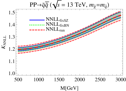
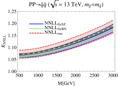
Refer to caption
Refer to caption
Refer to caption
Refer to caption
Figure 2: Resummation uncertainty for the NNLL resummed result with the default scale choice (2.55) (NNLLfixSZfixSZ{}_{\text{fixSZ}}, solid blue) compared to a running and a fixed soft scale determined as discussed in [16] (NNLLfixBNfixBN{}_{\text{fixBN}}, short dashed green, and NNLLrunrun{}_{\text{run}}, dashed red) for squark-antisquark (top-left), squark-squark (top-right), squark-gluino (bottom-left) and gluino-gluino (bottom-right) at LHC with s=13𝑠13\sqrt{s}=13\, TeV. The central lines represent the K𝐾K-factors for the default scale choice, while the bands give the resummation uncertainties associated with the results. See text for explanation.

In Figure 2 we compare the NNLL K-factors, defined in (3.2) below, and the resummation uncertainty for our default implementation with the fixed soft scale (2.55) to an implementation using a running scale, as in the previous NLL results in [16], and a fixed scale determined using the method of Becher and Neubert [60]. In the running-scale results the variation of μssubscript𝜇𝑠\mu_{s} in the resummation uncertainty is replaced by a variation of the parameters βcutsubscript𝛽cut\beta_{\text{cut}} and kssubscript𝑘𝑠k_{s} according to the procedure given in [51]. The curves do not include the C(2)superscript𝐶2C^{(2)} error estimate, which is common to all implementations. The central predictions obtained with the different scale-setting methods agree well for all production processes, while the estimate of the resummation uncertainty is larger for the running scale prescription. However, we find that the total theoretical uncertainty including factorization scale variation is similar for the three methods. Note that the agreement of the different scale choices is significantly improved compared to the NLL results (see Figure 6 in [16]). Therefore contrary to resummation at NLL level, we find that at NNLL the ambiguity in the choice of the soft scale prescription is negligible with respect to the total theoretical uncertainty.

3.2 Results

We present results for squark and gluino production at the LHC for five different higher-order approximations:

  • NNLL: the default implementation. Contains the full combined soft and Coulomb resummation, Eq. (2.10) including bound-state contributions (2.48) below threshold, matched to NNLOappapp{}_{\text{app}} according to (3.1). For the soft scale we adopt the fixed scale given in (2.55).

  • NNLLfixed-Cfixed-C{}_{\text{fixed-C}}: as above but using the fixed-order NNLO Coulomb terms (2.52) without bound-state effects interfering with resummed soft radiation, and for μh=μfsubscript𝜇subscript𝜇𝑓\mu_{h}=\mu_{f}.

  • NNLOappapp{}_{\text{app}}: The approximate NNLO corrections [53] including the spin-dependent non-Coulomb (2.47) and annihilation terms.

  • NLL: The NLL corrections from [16] with combined soft and Coulomb resummation and bound-state effects. Note that the scale choice (2.55) is used for the NLL results as well, whereas a running scale was used as the default in [16].

  • NLLs: Soft NLL resummation without Coulomb resummation and for μh=μfsubscript𝜇subscript𝜇𝑓\mu_{h}=\mu_{f}.

Refer to caption
Refer to caption
Refer to caption
Refer to caption
Figure 3: Higher-order corrections relative to the NLO cross section for squark and gluino production at the LHC with s=13𝑠13\sqrt{s}=13 TeV for full NNLL resummation (solid blue), NNLL with fixed-order Coulomb corrections (dotted red), approximate NNLO (dot-dashed pink), NLL (dashed orange) and NLL soft (long-dashed green). The PDF4LHC15_nnlo_30 PDFs are used throughout.

Our NNLL predictions for the LHC with s=13𝑠13\sqrt{s}=13 (141414 TeV) are provided as grids for mq~,mg~=200subscript𝑚~𝑞subscript𝑚~𝑔200m_{\tilde{q}},m_{\tilde{g}}=200300030003000 GeV (200200200350035003500 GeV) [1]. We also provide a Mathematica file with interpolations of the cross sections. As an illustration, our results for the four squark and gluino production processes at the LHC with s=13TeV𝑠13TeV\sqrt{s}=13\,\mathrm{TeV}666Results at s=8TeV𝑠8TeV\sqrt{s}=8\,\mathrm{TeV} have been presented in [19] for a slightly different setup using the running soft scale prescription, the MSTW08 PDFs and omitting the annihilation contribution. for equal squark and gluino masses are shown in Figure 3 in the form of K-factors beyond NLO,

KX=σXσNLO.subscript𝐾Xsubscript𝜎Xsubscript𝜎NLOK_{\text{X}}=\frac{\sigma_{\text{X}}}{\sigma_{\text{NLO}}}. (3.2)

Here X𝑋X denotes one of the approximations NLL, NNLLfixed-Cfixed-C{}_{\text{fixed-C}}, NNLOappapp{}_{\text{app}} and NNLL defined above and σNLOsubscript𝜎NLO\sigma_{\text{NLO}} is the fixed-order NLO result obtained using PROSPINO. We use the PDF4LHC15_nnlo PDFs for all results, including the NLO normalization in (3.2), in order to isolate the effects of the higher-order corrections to the partonic cross sections. The corrections relative to NLO can become large for the full NNLL resummation, ranging from up to 18%percent1818\% for squark-squark production to 90%percent9090\% for gluino pair production. Compared to the NLL results, the NNLL corrections provide a shift of the cross section by 10101020%percent2020\% normalized to the NLO prediction. This shows that a stabilization of the perturbative behaviour is achieved by the resummation, in particular for the processes with large corrections such as gluino-pair production. Note that this is only the case for the joint soft-Coulomb resummation performed here and in [12, 16], whereas a large NNLL correction is observed relative to the NLLs prediction that does not include Coulomb resummation. This observation is consistent with the results of Mellin-space resummation [20]. The effect of Coulomb resummation beyond NNLO and the bound-state effects can be seen by comparing the NNLL and NNLLfixed-CsubscriptNNLLfixed-C\text{NNLL}_{\text{fixed-C}} results and is important in particular for squark-antisquark and gluino-pair production. For squark-squark production, the effect of Coulomb resummation beyond NNLO is small. A similar behaviour was also observed for the NLL corrections beyond NLO in [16] and originates from cancellations between the negative corrections arising from the repulsive colour-sextet channel and the positive corrections arising from the attractive colour-triplet channel. The comparison to the approximate NNLO results shows that corrections beyond NNLO become sizeable beyond sparticle masses of about 1.51.51.5 TeV. The NNLLfixed-CsubscriptNNLLfixed-C\text{NNLL}_{\text{fixed-C}} correction factors in Figure 3 cannot be directly compared to the corresponding results using the Mellin-space formalism [20] that are given using the MSTW2008 set of PDFs. However, a comparison to our own earlier results for the NNLLfixed-CsubscriptNNLLfixed-C\text{NNLL}_{\text{fixed-C}} approximation at 8TeV8TeV8\,\mathrm{TeV} using the same PDFs [19] shows overall good agreement, which is reassuring given the different methods used for the resummation. As already noted in [20], the largest difference of order 10%percent1010\% appears for gluino pair-production at large masses, which is larger than the estimated resummation uncertainty of approximately 5%percent55\% of our result. Therefore, a more detailed comparison of the two approaches will be useful.
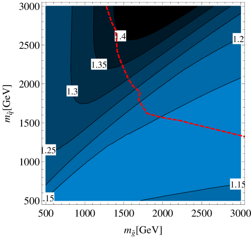
Refer to caption
Figure 4: NNLL K𝐾K-factor for the total SUSY pair production rate at the LHC with s=13𝑠13\sqrt{s}=13 TeV, as a function of the squark mass mq~subscript𝑚~𝑞m_{\tilde{q}} and gluino mass mg~subscript𝑚~𝑔m_{\tilde{g}}. The red, dashed line is the ATLAS exclusion bound from searches at s=8𝑠8\sqrt{s}=8 TeV in a simplified model with a massless neutralino [2].

Figure 4 shows the NNLL K𝐾K-factor for the total SUSY production rate, i.e. the sum of all squark and gluino pair production processes, at the 131313 TeV LHC as a contour plot in the (mg~,mq~)subscript𝑚~𝑔subscript𝑚~𝑞(m_{\tilde{g}},m_{\tilde{q}})-plane. The NNLL corrections are larger in the region with mg~<mq~subscript𝑚~𝑔subscript𝑚~𝑞m_{\tilde{g}}<m_{\tilde{q}} where squark-gluino and gluino-pair production with the corresponding larger K𝐾K-factors dominate the total SUSY production rate, see e.g. [16]. In contrast, for mq~mg~subscript𝑚~𝑞subscript𝑚~𝑔m_{\tilde{q}}\leq m_{\tilde{g}} the total rate is dominated by squark-squark production with a resulting smaller K𝐾K-factor. Since squark-antisquark production is suppressed compared to squark-squark production at the LHC unless mg~mq~much-greater-thansubscript𝑚~𝑔subscript𝑚~𝑞m_{\tilde{g}}\gg m_{\tilde{q}}, the large K𝐾K-factor in this process has little impact on the total SUSY production rate for the mass range considered in Fig. 4. For illustration, the plot also shows a Run 1 ATLAS exclusion bound in a simplified model with a massless neutralino [2] that shows that corrections larger than 40%percent4040\% arise in a region relevant for current searches.
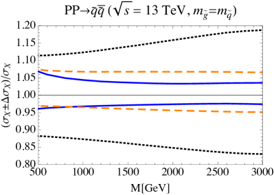
Refer to caption
Refer to caption
Refer to caption
Refer to caption
Figure 5: Total theoretical uncertainty (excluding PDF uncertainty) of the NLO approximation (dotted black), NLL (dashed orange) and NNLL (solid blue) resummed results at the LHC with s= 13𝑠13\sqrt{s}=\,13 TeV. The uncertainty estimate is given by the scale uncertainty, the resummation uncertainty (for NLL and NNLL) and the estimate of missing higher-order corrections (for NNLL). All cross sections are normalized to the one at the central value of the scales.

The estimate of the theory uncertainty of the NLO, NLL and NNLL approximations is shown in Figure 5, normalized to the central value of the respective prediction. Following the discussion in Section 3.1, the NLO uncertainty is estimated by the factorization scale variation, the NLL uncertainty includes in addition the estimate of the resummation ambiguities and the NNLL uncertainty further includes the estimate of the two-loop constant. The PDF+αssubscript𝛼𝑠+\alpha_{s} uncertainty is not included in the results shown in Figure 5. One observes that the uncertainty is reduced from up to 20%percent2020\% at NLO to the 10%percent1010\% level at NLL. While a significant reduction of the uncertainty compared to the NLL results is observed for the squark-antisquark production process at NNLL, only a slight reduction or even an increase is observed for the other processes. We further investigate the different sources of uncertainties in Figure 6 and Table 7 below, where it is seen that this behaviour is due to the scale uncertainty, while the resummation uncertainty is generally reduced at NNLL.

mq~subscript𝑚~𝑞m_{\tilde{q}}, mg~(TeV)subscript𝑚~𝑔TeVm_{\tilde{g}}\,(\mathrm{TeV}) s~s~~𝑠superscript~𝑠\tilde{s}\tilde{s}^{\prime} σNLO(pb)subscript𝜎NLOpb\sigma_{\mathrm{NLO}}(\mathrm{pb}) σNLL(pb)subscript𝜎NLLpb\sigma_{\mathrm{NLL}}(\mathrm{pb}) σNNLL(pb)subscript𝜎NNLLpb\sigma_{\mathrm{NNLL}}(\mathrm{pb}) KNNLLsubscript𝐾NNLLK_{\text{NNLL}}
1.31.31.3, 1.51.51.5 q~q~¯~𝑞¯~𝑞\tilde{q}\bar{\tilde{q}} 2.810.37+0.36×0.18+0.181022.81_{-0.37}^{+0.36}{}_{-0.18}^{+0.18}\times 10^{-2} 3.060.11+0.19×0.19+0.191023.06_{-0.11}^{+0.19}{}_{-0.19}^{+0.19}\times 10^{-2} 3.490.09+0.13×0.20+0.201023.49_{-0.09}^{+0.13}{}_{-0.20}^{+0.20}\times 10^{-2} 1.241.241.24
q~q~~𝑞~𝑞\tilde{q}\tilde{q} 8.640.90+0.74×0.25+0.251028.64_{-0.90}^{+0.74}{}_{-0.25}^{+0.25}\times 10^{-2} 8.760.55+0.76×0.25+0.251028.76_{-0.55}^{+0.76}{}_{-0.25}^{+0.25}\times 10^{-2} 9.370.53+0.56×0.26+0.261029.37_{-0.53}^{+0.56}{}_{-0.26}^{+0.26}\times 10^{-2} 1.081.081.08
q~g~~𝑞~𝑔\tilde{q}\tilde{g} 7.250.86+0.62×0.50+0.501027.25_{-0.86}^{+0.62}{}_{-0.50}^{+0.50}\times 10^{-2} 7.930.37+0.28×0.51+0.511027.93_{-0.37}^{+0.28}{}_{-0.51}^{+0.51}\times 10^{-2} 8.490.46+0.43×0.52+0.521028.49_{-0.46}^{+0.43}{}_{-0.52}^{+0.52}\times 10^{-2} 1.171.171.17
g~g~~𝑔~𝑔\tilde{g}\tilde{g} 6.391.01+0.88×1.34+1.341036.39_{-1.01}^{+0.88}{}_{-1.34}^{+1.34}\times 10^{-3} 8.030.66+0.81×1.37+1.371038.03_{-0.66}^{+0.81}{}_{-1.37}^{+1.37}\times 10^{-3} 8.710.89+0.82×1.40+1.401038.71_{-0.89}^{+0.82}{}_{-1.40}^{+1.40}\times 10^{-3} 1.361.361.36
1.51.51.5, 1.31.31.3 q~q~¯~𝑞¯~𝑞\tilde{q}\bar{\tilde{q}} 9.331.26+1.23×0.70+0.701039.33_{-1.26}^{+1.23}{}_{-0.70}^{+0.70}\times 10^{-3} 1.020.04+0.06×0.07+0.071021.02_{-0.04}^{+0.06}{}_{-0.07}^{+0.07}\times 10^{-2} 1.170.04+0.05×0.08+0.081021.17_{-0.04}^{+0.05}{}_{-0.08}^{+0.08}\times 10^{-2} 1.251.251.25
q~q~~𝑞~𝑞\tilde{q}\tilde{q} 4.200.50+0.47×0.13+0.131024.20_{-0.50}^{+0.47}{}_{-0.13}^{+0.13}\times 10^{-2} 4.250.35+0.46×0.13+0.131024.25_{-0.35}^{+0.46}{}_{-0.13}^{+0.13}\times 10^{-2} 4.580.44+0.47×0.14+0.141024.58_{-0.44}^{+0.47}{}_{-0.14}^{+0.14}\times 10^{-2} 1.091.091.09
q~g~~𝑞~𝑔\tilde{q}\tilde{g} 8.701.15+0.97×0.600.601028.70_{-1.15}^{+0.97}{}_{-0.60}^{0.60}\times 10^{-2} 9.590.47+0.35×0.61+0.611029.59_{-0.47}^{+0.35}{}_{-0.61}^{+0.61}\times 10^{-2} 1.060.05+0.06×0.06+0.061011.06_{-0.05}^{+0.06}{}_{-0.06}^{+0.06}\times 10^{-1} 1.221.221.22
g~g~~𝑔~𝑔\tilde{g}\tilde{g} 2.450.40+0.38×0.42+0.421022.45_{-0.40}^{+0.38}{}_{-0.42}^{+0.42}\times 10^{-2} 2.970.19+0.24×0.43+0.431022.97_{-0.19}^{+0.24}{}_{-0.43}^{+0.43}\times 10^{-2} 3.360.22+0.22×0.45+0.451023.36_{-0.22}^{+0.22}{}_{-0.45}^{+0.45}\times 10^{-2} 1.371.371.37
1.81.81.8, 222 q~q~¯~𝑞¯~𝑞\tilde{q}\bar{\tilde{q}} 1.660.24+0.24×0.17+0.171031.66_{-0.24}^{+0.24}{}_{-0.17}^{+0.17}\times 10^{-3} 1.870.08+0.12×0.18+0.181031.87_{-0.08}^{+0.12}{}_{-0.18}^{+0.18}\times 10^{-3} 2.160.05+0.07×0.19+0.191032.16_{-0.05}^{+0.07}{}_{-0.19}^{+0.19}\times 10^{-3} 1.301.301.30
q~q~~𝑞~𝑞\tilde{q}\tilde{q} 9.611.13+0.99×0.34+0.341039.61_{-1.13}^{+0.99}{}_{-0.34}^{+0.34}\times 10^{-3} 9.820.68+0.92×0.34+0.341039.82_{-0.68}^{+0.92}{}_{-0.34}^{+0.34}\times 10^{-3} 1.060.06+0.07×0.04+0.041021.06_{-0.06}^{+0.07}{}_{-0.04}^{+0.04}\times 10^{-2} 1.111.111.11
q~g~~𝑞~𝑔\tilde{q}\tilde{g} 5.150.69+0.54×0.59+0.591035.15_{-0.69}^{+0.54}{}_{-0.59}^{+0.59}\times 10^{-3} 5.860.35+0.27×0.60+0.601035.86_{-0.35}^{+0.27}{}_{-0.60}^{+0.60}\times 10^{-3} 6.340.39+0.36×0.60+0.601036.34_{-0.39}^{+0.36}{}_{-0.60}^{+0.60}\times 10^{-3} 1.231.231.23
g~g~~𝑔~𝑔\tilde{g}\tilde{g} 3.180.56+0.51×1.05+1.051043.18_{-0.56}^{+0.51}{}_{-1.05}^{+1.05}\times 10^{-4} 4.330.45+0.52×1.08+1.081044.33_{-0.45}^{+0.52}{}_{-1.08}^{+1.08}\times 10^{-4} 4.710.54+0.50×1.12+1.121044.71_{-0.54}^{+0.50}{}_{-1.12}^{+1.12}\times 10^{-4} 1.481.481.48
222, 1.81.81.8 q~q~¯~𝑞¯~𝑞\tilde{q}\bar{\tilde{q}} 5.840.87+0.88×0.79+0.791045.84_{-0.87}^{+0.88}{}_{-0.79}^{+0.79}\times 10^{-4} 6.620.28+0.42×0.80+0.801046.62_{-0.28}^{+0.42}{}_{-0.80}^{+0.80}\times 10^{-4} 7.690.23+0.27×0.85+0.851047.69_{-0.23}^{+0.27}{}_{-0.85}^{+0.85}\times 10^{-4} 1.321.321.32
q~q~~𝑞~𝑞\tilde{q}\tilde{q} 4.680.61+0.58×0.19+0.191034.68_{-0.61}^{+0.58}{}_{-0.19}^{+0.19}\times 10^{-3} 4.780.40+0.53×0.19+0.191034.78_{-0.40}^{+0.53}{}_{-0.19}^{+0.19}\times 10^{-3} 5.230.45+0.49×0.19+0.191035.23_{-0.45}^{+0.49}{}_{-0.19}^{+0.19}\times 10^{-3} 1.121.121.12
q~g~~𝑞~𝑔\tilde{q}\tilde{g} 5.960.86+0.76×0.68+0.681035.96_{-0.86}^{+0.76}{}_{-0.68}^{+0.68}\times 10^{-3} 6.820.41+0.28×0.69+0.691036.82_{-0.41}^{+0.28}{}_{-0.69}^{+0.69}\times 10^{-3} 7.620.44+0.46×0.70+0.701037.62_{-0.44}^{+0.46}{}_{-0.70}^{+0.70}\times 10^{-3} 1.281.281.28
g~g~~𝑔~𝑔\tilde{g}\tilde{g} 1.070.19+0.19×0.30+0.301031.07_{-0.19}^{+0.19}{}_{-0.30}^{+0.30}\times 10^{-3} 1.400.11+0.14×0.30+0.301031.40_{-0.11}^{+0.14}{}_{-0.30}^{+0.30}\times 10^{-3} 1.600.13+0.13×0.32+0.321031.60_{-0.13}^{+0.13}{}_{-0.32}^{+0.32}\times 10^{-3} 1.491.491.49
2.32.32.3, 2.52.52.5 q~q~¯~𝑞¯~𝑞\tilde{q}\bar{\tilde{q}} 1.130.18+0.19×0.24+0.241041.13_{-0.18}^{+0.19}{}_{-0.24}^{+0.24}\times 10^{-4} 1.320.06+0.09×0.25+0.251041.32_{-0.06}^{+0.09}{}_{-0.25}^{+0.25}\times 10^{-4} 1.550.04+0.05×0.26+0.261041.55_{-0.04}^{+0.05}{}_{-0.26}^{+0.26}\times 10^{-4} 1.371.371.37
q~q~~𝑞~𝑞\tilde{q}\tilde{q} 1.180.15+0.14×0.06+0.061031.18_{-0.15}^{+0.14}{}_{-0.06}^{+0.06}\times 10^{-3} 1.210.09+0.12×0.06+0.061031.21_{-0.09}^{+0.12}{}_{-0.06}^{+0.06}\times 10^{-3} 1.330.08+0.09×0.06+0.061031.33_{-0.08}^{+0.09}{}_{-0.06}^{+0.06}\times 10^{-3} 1.131.131.13
q~g~~𝑞~𝑔\tilde{q}\tilde{g} 4.290.65+0.55×0.77+0.771044.29_{-0.65}^{+0.55}{}_{-0.77}^{+0.77}\times 10^{-4} 5.130.37+0.30×0.78+0.781045.13_{-0.37}^{+0.30}{}_{-0.78}^{+0.78}\times 10^{-4} 5.600.39+0.37×0.79+0.791045.60_{-0.39}^{+0.37}{}_{-0.79}^{+0.79}\times 10^{-4} 1.311.311.31
g~g~~𝑔~𝑔\tilde{g}\tilde{g} 1.880.36+0.36×0.93+0.931051.88_{-0.36}^{+0.36}{}_{-0.93}^{+0.93}\times 10^{-5} 2.840.36+0.41×0.98+0.981052.84_{-0.36}^{+0.41}{}_{-0.98}^{+0.98}\times 10^{-5} 3.110.39+0.38×1.04+1.041053.11_{-0.39}^{+0.38}{}_{-1.04}^{+1.04}\times 10^{-5} 1.651.651.65
2.52.52.5, 2.32.32.3 q~q~¯~𝑞¯~𝑞\tilde{q}\bar{\tilde{q}} 3.980.64+0.68×1.27+1.271053.98_{-0.64}^{+0.68}{}_{-1.27}^{+1.27}\times 10^{-5} 4.720.22+0.30×1.29+1.291054.72_{-0.22}^{+0.30}{}_{-1.29}^{+1.29}\times 10^{-5} 5.560.15+0.20×1.36+1.361055.56_{-0.15}^{+0.20}{}_{-1.36}^{+1.36}\times 10^{-5} 1.401.401.40
q~q~~𝑞~𝑞\tilde{q}\tilde{q} 5.550.79+0.77×0.33+0.331045.55_{-0.79}^{+0.77}{}_{-0.33}^{+0.33}\times 10^{-4} 5.740.48+0.65×0.33+0.331045.74_{-0.48}^{+0.65}{}_{-0.33}^{+0.33}\times 10^{-4} 6.360.51+0.56×0.33+0.331046.36_{-0.51}^{+0.56}{}_{-0.33}^{+0.33}\times 10^{-4} 1.151.151.15
q~g~~𝑞~𝑔\tilde{q}\tilde{g} 4.840.77+0.71×0.86+0.861044.84_{-0.77}^{+0.71}{}_{-0.86}^{+0.86}\times 10^{-4} 5.830.41+0.31×0.88+0.881045.83_{-0.41}^{+0.31}{}_{-0.88}^{+0.88}\times 10^{-4} 6.560.43+0.45×0.90+0.901046.56_{-0.43}^{+0.45}{}_{-0.90}^{+0.90}\times 10^{-4} 1.361.361.36
g~g~~𝑔~𝑔\tilde{g}\tilde{g} 6.071.20+1.25×2.56+2.561056.07_{-1.20}^{+1.25}{}_{-2.56}^{+2.56}\times 10^{-5} 8.620.85+1.03×2.66+2.661058.62_{-0.85}^{+1.03}{}_{-2.66}^{+2.66}\times 10^{-5} 1.000.09+0.10×0.28+0.281041.00_{-0.09}^{+0.10}{}_{-0.28}^{+0.28}\times 10^{-4} 1.651.651.65
2.82.82.8, 333 q~q~¯~𝑞¯~𝑞\tilde{q}\bar{\tilde{q}} 7.941.33+1.45×4.56+4.561067.94_{-1.33}^{+1.45}{}_{-4.56}^{+4.56}\times 10^{-6} 9.690.48+0.63×4.65+4.651069.69_{-0.48}^{+0.63}{}_{-4.65}^{+4.65}\times 10^{-6} 1.150.03+0.04×0.48+0.481051.15_{-0.03}^{+0.04}{}_{-0.48}^{+0.48}\times 10^{-5} 1.451.451.45
q~q~~𝑞~𝑞\tilde{q}\tilde{q} 1.410.20+0.19×0.11+0.111041.41_{-0.20}^{+0.19}{}_{-0.11}^{+0.11}\times 10^{-4} 1.470.11+0.15×0.11+0.111041.47_{-0.11}^{+0.15}{}_{-0.11}^{+0.11}\times 10^{-4} 1.640.10+0.11×0.11+0.111041.64_{-0.10}^{+0.11}{}_{-0.11}^{+0.11}\times 10^{-4} 1.171.171.17
q~g~~𝑞~𝑔\tilde{q}\tilde{g} 3.620.61+0.56×0.97+0.971053.62_{-0.61}^{+0.56}{}_{-0.97}^{+0.97}\times 10^{-5} 4.620.40+0.32×0.99+0.991054.62_{-0.40}^{+0.32}{}_{-0.99}^{+0.99}\times 10^{-5} 5.100.41+0.37×1.01+1.011055.10_{-0.41}^{+0.37}{}_{-1.01}^{+1.01}\times 10^{-5} 1.411.411.41
g~g~~𝑔~𝑔\tilde{g}\tilde{g} 1.150.24+0.25×0.82+0.821061.15_{-0.24}^{+0.25}{}_{-0.82}^{+0.82}\times 10^{-6} 1.970.31+0.33×0.92+0.921061.97_{-0.31}^{+0.33}{}_{-0.92}^{+0.92}\times 10^{-6} 2.180.31+0.29×1.01+1.011062.18_{-0.31}^{+0.29}{}_{-1.01}^{+1.01}\times 10^{-6} 1.901.901.90
333, 2.82.82.8 q~q~¯~𝑞¯~𝑞\tilde{q}\bar{\tilde{q}} 2.830.47+0.51×2.53+2.531062.83_{-0.47}^{+0.51}{}_{-2.53}^{+2.53}\times 10^{-6} 3.500.17+0.22×2.56+2.561063.50_{-0.17}^{+0.22}{}_{-2.56}^{+2.56}\times 10^{-6} 4.170.12+0.15×2.63+2.631064.17_{-0.12}^{+0.15}{}_{-2.63}^{+2.63}\times 10^{-6} 1.471.471.47
q~q~~𝑞~𝑞\tilde{q}\tilde{q} 6.280.96+0.98×0.60+0.601056.28_{-0.96}^{+0.98}{}_{-0.60}^{+0.60}\times 10^{-5} 6.610.56+0.77×0.59+0.591056.61_{-0.56}^{+0.77}{}_{-0.59}^{+0.59}\times 10^{-5} 7.430.56+0.61×0.59+0.591057.43_{-0.56}^{+0.61}{}_{-0.59}^{+0.59}\times 10^{-5} 1.181.181.18
q~g~~𝑞~𝑔\tilde{q}\tilde{g} 4.020.71+0.69×1.08+1.081054.02_{-0.71}^{+0.69}{}_{-1.08}^{+1.08}\times 10^{-5} 5.160.43+0.34×1.10+1.101055.16_{-0.43}^{+0.34}{}_{-1.10}^{+1.10}\times 10^{-5} 5.870.44+0.44×1.13+1.131055.87_{-0.44}^{+0.44}{}_{-1.13}^{+1.13}\times 10^{-5} 1.461.461.46
g~g~~𝑔~𝑔\tilde{g}\tilde{g} 3.700.80+0.88×2.27+2.271063.70_{-0.80}^{+0.88}{}_{-2.27}^{+2.27}\times 10^{-6} 5.900.73+0.85×2.45+2.451065.90_{-0.73}^{+0.85}{}_{-2.45}^{+2.45}\times 10^{-6} 6.940.76+0.78×2.70+2.701066.94_{-0.76}^{+0.78}{}_{-2.70}^{+2.70}\times 10^{-6} 1.871.871.87
Table 5: Predictions for the LHC with s=13𝑠13\sqrt{s}=13 TeV using the PDF4LHC15_nnlo_30 PDFs. The first and second error refer to the theoretical uncertainty, defined as in Figure 5, and the PDF+αssubscript𝛼𝑠+\alpha_{s} uncertainty, respectively.
mq~subscript𝑚~𝑞m_{\tilde{q}}, mg~(TeV)subscript𝑚~𝑔TeVm_{\tilde{g}}\,(\mathrm{TeV}) s~s~~𝑠superscript~𝑠\tilde{s}\tilde{s}^{\prime} σNLO(pb)subscript𝜎NLOpb\sigma_{\mathrm{NLO}}(\mathrm{pb}) σNLL(pb)subscript𝜎NLLpb\sigma_{\mathrm{NLL}}(\mathrm{pb}) σNNLL(pb)subscript𝜎NNLLpb\sigma_{\mathrm{NNLL}}(\mathrm{pb}) KNNLLsubscript𝐾NNLLK_{\text{NNLL}}
1.8,21.821.8,2 q~q~¯~𝑞¯~𝑞\tilde{q}\bar{\tilde{q}} 2.820.40+0.40×0.26+0.261032.82_{-0.40}^{+0.40}{}_{-0.26}^{+0.26}\times 10^{-3} 3.140.13+0.20×0.26+0.261033.14_{-0.13}^{+0.20}{}_{-0.26}^{+0.26}\times 10^{-3} 3.610.09+0.12×0.28+0.281033.61_{-0.09}^{+0.12}{}_{-0.28}^{+0.28}\times 10^{-3} 1.281.281.28
q~q~~𝑞~𝑞\tilde{q}\tilde{q} 1.400.16+0.14×0.05+0.051021.40_{-0.16}^{+0.14}{}_{-0.05}^{+0.05}\times 10^{-2} 1.430.10+0.13×0.05+0.051021.43_{-0.10}^{+0.13}{}_{-0.05}^{+0.05}\times 10^{-2} 1.540.09+0.10×0.05+0.051021.54_{-0.09}^{+0.10}{}_{-0.05}^{+0.05}\times 10^{-2} 1.101.101.10
q~g~~𝑞~𝑔\tilde{q}\tilde{g} 8.611.11+0.85×0.86+0.861038.61_{-1.11}^{+0.85}{}_{-0.86}^{+0.86}\times 10^{-3} 9.680.53+0.41×0.87+0.871039.68_{-0.53}^{+0.41}{}_{-0.87}^{+0.87}\times 10^{-3} 1.040.06+0.06×0.09+0.091021.04_{-0.06}^{+0.06}{}_{-0.09}^{+0.09}\times 10^{-2} 1.211.211.21
g~g~~𝑔~𝑔\tilde{g}\tilde{g} 6.021.01+0.91×1.75+1.751046.02_{-1.01}^{+0.91}{}_{-1.75}^{+1.75}\times 10^{-4} 7.970.78+0.91×1.80+1.801047.97_{-0.78}^{+0.91}{}_{-1.80}^{+1.80}\times 10^{-4} 8.630.96+0.89×1.84+1.841048.63_{-0.96}^{+0.89}{}_{-1.84}^{+1.84}\times 10^{-4} 1.441.441.44
2.,1.82.,1.8 q~q~¯~𝑞¯~𝑞\tilde{q}\bar{\tilde{q}} 1.060.15+0.15×0.12+0.121031.06_{-0.15}^{+0.15}{}_{-0.12}^{+0.12}\times 10^{-3} 1.190.05+0.07×0.12+0.121031.19_{-0.05}^{+0.07}{}_{-0.12}^{+0.12}\times 10^{-3} 1.370.04+0.05×0.13+0.131031.37_{-0.04}^{+0.05}{}_{-0.13}^{+0.13}\times 10^{-3} 1.291.291.29
q~q~~𝑞~𝑞\tilde{q}\tilde{q} 7.200.90+0.85×0.26+0.261037.20_{-0.90}^{+0.85}{}_{-0.26}^{+0.26}\times 10^{-3} 7.340.59+0.80×0.26+0.261037.34_{-0.59}^{+0.80}{}_{-0.26}^{+0.26}\times 10^{-3} 7.980.70+0.75×0.27+0.271037.98_{-0.70}^{+0.75}{}_{-0.27}^{+0.27}\times 10^{-3} 1.111.111.11
q~g~~𝑞~𝑔\tilde{q}\tilde{g} 9.941.39+1.20×0.99+0.991039.94_{-1.39}^{+1.20}{}_{-0.99}^{+0.99}\times 10^{-3} 1.120.06+0.04×0.10+0.101021.12_{-0.06}^{+0.04}{}_{-0.10}^{+0.10}\times 10^{-2} 1.250.07+0.07×0.10+0.101021.25_{-0.07}^{+0.07}{}_{-0.10}^{+0.10}\times 10^{-2} 1.261.261.26
g~g~~𝑔~𝑔\tilde{g}\tilde{g} 1.910.33+0.32×0.47+0.471031.91_{-0.33}^{+0.32}{}_{-0.47}^{+0.47}\times 10^{-3} 2.430.18+0.22×0.48+0.481032.43_{-0.18}^{+0.22}{}_{-0.48}^{+0.48}\times 10^{-3} 2.770.21+0.21×0.50+0.501032.77_{-0.21}^{+0.21}{}_{-0.50}^{+0.50}\times 10^{-3} 1.451.451.45
2.3,2.52.32.52.3,2.5 q~q~¯~𝑞¯~𝑞\tilde{q}\bar{\tilde{q}} 2.280.35+0.36×0.38+0.381042.28_{-0.35}^{+0.36}{}_{-0.38}^{+0.38}\times 10^{-4} 2.620.12+0.17×0.38+0.381042.62_{-0.12}^{+0.17}{}_{-0.38}^{+0.38}\times 10^{-4} 3.050.07+0.10×0.41+0.411043.05_{-0.07}^{+0.10}{}_{-0.41}^{+0.41}\times 10^{-4} 1.34
q~q~~𝑞~𝑞\tilde{q}\tilde{q} 1.960.25+0.22×0.09+0.091031.96_{-0.25}^{+0.22}{}_{-0.09}^{+0.09}\times 10^{-3} 2.020.14+0.20×0.09+0.091032.02_{-0.14}^{+0.20}{}_{-0.09}^{+0.09}\times 10^{-3} 2.200.13+0.14×0.09+0.091032.20_{-0.13}^{+0.14}{}_{-0.09}^{+0.09}\times 10^{-3} 1.121.121.12
q~g~~𝑞~𝑔\tilde{q}\tilde{g} 8.311.20+0.99×1.27+1.271048.31_{-1.20}^{+0.99}{}_{-1.27}^{+1.27}\times 10^{-4} 9.750.65+0.52×1.29+1.291049.75_{-0.65}^{+0.52}{}_{-1.29}^{+1.29}\times 10^{-4} 1.060.07+0.07×0.13+0.131031.06_{-0.07}^{+0.07}{}_{-0.13}^{+0.13}\times 10^{-3} 1.281.281.28
g~g~~𝑔~𝑔\tilde{g}\tilde{g} 4.210.78+0.74×1.81+1.811054.21_{-0.78}^{+0.74}{}_{-1.81}^{+1.81}\times 10^{-5} 6.080.72+0.83×1.88+1.881056.08_{-0.72}^{+0.83}{}_{-1.88}^{+1.88}\times 10^{-5} 6.640.79+0.77×1.97+1.971056.64_{-0.79}^{+0.77}{}_{-1.97}^{+1.97}\times 10^{-5} 1.581.581.58
2.5,2.32.52.32.5,2.3 q~q~¯~𝑞¯~𝑞\tilde{q}\bar{\tilde{q}} 8.621.34+1.40×1.96+1.961058.62_{-1.34}^{+1.40}{}_{-1.96}^{+1.96}\times 10^{-5} 1.000.04+0.06×0.20+0.201041.00_{-0.04}^{+0.06}{}_{-0.20}^{+0.20}\times 10^{-4} 1.180.03+0.04×0.21+0.211041.18_{-0.03}^{+0.04}{}_{-0.21}^{+0.21}\times 10^{-4} 1.361.361.36
q~q~~𝑞~𝑞\tilde{q}\tilde{q} 9.891.34+1.30×0.50+0.501049.89_{-1.34}^{+1.30}{}_{-0.50}^{+0.50}\times 10^{-4} 1.020.08+0.11×0.05+0.051031.02_{-0.08}^{+0.11}{}_{-0.05}^{+0.05}\times 10^{-3} 1.120.09+0.10×0.05+0.051031.12_{-0.09}^{+0.10}{}_{-0.05}^{+0.05}\times 10^{-3} 1.131.131.13
q~g~~𝑞~𝑔\tilde{q}\tilde{g} 9.381.43+1.29×1.43+1.431049.38_{-1.43}^{+1.29}{}_{-1.43}^{+1.43}\times 10^{-4} 1.110.07+0.05×0.15+0.151031.11_{-0.07}^{+0.05}{}_{-0.15}^{+0.15}\times 10^{-3} 1.240.08+0.08×0.15+0.151031.24_{-0.08}^{+0.08}{}_{-0.15}^{+0.15}\times 10^{-3} 1.321.321.32
g~g~~𝑔~𝑔\tilde{g}\tilde{g} 1.270.24+0.24×0.46+0.461041.27_{-0.24}^{+0.24}{}_{-0.46}^{+0.46}\times 10^{-4} 1.740.16+0.19×0.48+0.481041.74_{-0.16}^{+0.19}{}_{-0.48}^{+0.48}\times 10^{-4} 2.000.17+0.18×0.50+0.501042.00_{-0.17}^{+0.18}{}_{-0.50}^{+0.50}\times 10^{-4} 1.581.581.58
2.8,32.832.8,3 q~q~¯~𝑞¯~𝑞\tilde{q}\bar{\tilde{q}} 1.910.31+0.34×0.73+0.731051.91_{-0.31}^{+0.34}{}_{-0.73}^{+0.73}\times 10^{-5} 2.290.11+0.15×0.74+0.741052.29_{-0.11}^{+0.15}{}_{-0.74}^{+0.74}\times 10^{-5} 2.700.06+0.09×0.78+0.781052.70_{-0.06}^{+0.09}{}_{-0.78}^{+0.78}\times 10^{-5} 1.411.411.41
q~q~~𝑞~𝑞\tilde{q}\tilde{q} 2.770.38+0.36×0.18+0.181042.77_{-0.38}^{+0.36}{}_{-0.18}^{+0.18}\times 10^{-4} 2.880.22+0.29×0.18+0.181042.88_{-0.22}^{+0.29}{}_{-0.18}^{+0.18}\times 10^{-4} 3.190.19+0.21×0.18+0.181043.19_{-0.19}^{+0.21}{}_{-0.18}^{+0.18}\times 10^{-4} 1.151.151.15
q~g~~𝑞~𝑔\tilde{q}\tilde{g} 8.411.35+1.19×1.91+1.911058.41_{-1.35}^{+1.19}{}_{-1.91}^{+1.91}\times 10^{-5} 1.040.08+0.07×0.19+0.191041.04_{-0.08}^{+0.07}{}_{-0.19}^{+0.19}\times 10^{-4} 1.140.09+0.08×0.20+0.201041.14_{-0.09}^{+0.08}{}_{-0.20}^{+0.20}\times 10^{-4} 1.361.361.36
g~g~~𝑔~𝑔\tilde{g}\tilde{g} 3.130.63+0.64×1.91+1.911063.13_{-0.63}^{+0.64}{}_{-1.91}^{+1.91}\times 10^{-6} 5.050.72+0.79×2.07+2.071065.05_{-0.72}^{+0.79}{}_{-2.07}^{+2.07}\times 10^{-6} 5.560.75+0.70×2.23+2.231065.56_{-0.75}^{+0.70}{}_{-2.23}^{+2.23}\times 10^{-6} 1.781.781.78
3.,2.83.,2.8 q~q~¯~𝑞¯~𝑞\tilde{q}\bar{\tilde{q}} 7.241.18+1.27×4.15+4.151067.24_{-1.18}^{+1.27}{}_{-4.15}^{+4.15}\times 10^{-6} 8.780.42+0.55×4.22+4.221068.78_{-0.42}^{+0.55}{}_{-4.22}^{+4.22}\times 10^{-6} 1.040.03+0.04×0.44+0.441051.04_{-0.03}^{+0.04}{}_{-0.44}^{+0.44}\times 10^{-5} 1.441.441.44
q~q~~𝑞~𝑞\tilde{q}\tilde{q} 1.340.20+0.20×0.10+0.101041.34_{-0.20}^{+0.20}{}_{-0.10}^{+0.10}\times 10^{-4} 1.400.12+0.16×0.10+0.101041.40_{-0.12}^{+0.16}{}_{-0.10}^{+0.10}\times 10^{-4} 1.560.12+0.13×0.10+0.101041.56_{-0.12}^{+0.13}{}_{-0.10}^{+0.10}\times 10^{-4} 1.161.161.16
q~g~~𝑞~𝑔\tilde{q}\tilde{g} 9.341.56+1.48×2.12+2.121059.34_{-1.56}^{+1.48}{}_{-2.12}^{+2.12}\times 10^{-5} 1.160.09+0.07×0.21+0.211041.16_{-0.09}^{+0.07}{}_{-0.21}^{+0.21}\times 10^{-4} 1.310.10+0.09×0.22+0.221041.31_{-0.10}^{+0.09}{}_{-0.22}^{+0.22}\times 10^{-4} 1.411.411.41
g~g~~𝑔~𝑔\tilde{g}\tilde{g} 9.301.92+2.05×4.90+4.901069.30_{-1.92}^{+2.05}{}_{-4.90}^{+4.90}\times 10^{-6} 1.400.16+0.19×0.52+0.521051.40_{-0.16}^{+0.19}{}_{-0.52}^{+0.52}\times 10^{-5} 1.640.17+0.17×0.56+0.561051.64_{-0.17}^{+0.17}{}_{-0.56}^{+0.56}\times 10^{-5} 1.761.761.76
3.3,3.53.33.53.3,3.5 q~q~¯~𝑞¯~𝑞\tilde{q}\bar{\tilde{q}} 1.680.28+0.31×1.66+1.661061.68_{-0.28}^{+0.31}{}_{-1.66}^{+1.66}\times 10^{-6} 2.070.10+0.13×1.68+1.681062.07_{-0.10}^{+0.13}{}_{-1.68}^{+1.68}\times 10^{-6} 2.460.06+0.08×1.73+1.731062.46_{-0.06}^{+0.08}{}_{-1.73}^{+1.73}\times 10^{-6} 1.471.471.47
q~q~~𝑞~𝑞\tilde{q}\tilde{q} 3.680.55+0.54×0.38+0.381053.68_{-0.55}^{+0.54}{}_{-0.38}^{+0.38}\times 10^{-5} 3.890.30+0.41×0.37+0.371053.89_{-0.30}^{+0.41}{}_{-0.37}^{+0.37}\times 10^{-5} 4.350.26+0.28×0.37+0.371054.35_{-0.26}^{+0.28}{}_{-0.37}^{+0.37}\times 10^{-5} 1.181.181.18
q~g~~𝑞~𝑔\tilde{q}\tilde{g} 8.181.44+1.37×2.68+2.681068.18_{-1.44}^{+1.37}{}_{-2.68}^{+2.68}\times 10^{-6} 1.080.10+0.08×0.27+0.271051.08_{-0.10}^{+0.08}{}_{-0.27}^{+0.27}\times 10^{-5} 1.200.10+0.09×0.28+0.281051.20_{-0.10}^{+0.09}{}_{-0.28}^{+0.28}\times 10^{-5} 1.471.471.47
g~g~~𝑔~𝑔\tilde{g}\tilde{g} 2.280.50+0.53×1.90+1.901072.28_{-0.50}^{+0.53}{}_{-1.90}^{+1.90}\times 10^{-7} 4.190.69+0.74×2.26+2.261074.19_{-0.69}^{+0.74}{}_{-2.26}^{+2.26}\times 10^{-7} 4.650.69+0.66×2.55+2.551074.65_{-0.69}^{+0.66}{}_{-2.55}^{+2.55}\times 10^{-7} 2.042.042.04
3.5,3.33.53.33.5,3.3 q~q~¯~𝑞¯~𝑞\tilde{q}\bar{\tilde{q}} 6.721.11+1.20×9.60+9.601076.72_{-1.11}^{+1.20}{}_{-9.60}^{+9.60}\times 10^{-7} 8.320.39+0.52×9.65+9.651078.32_{-0.39}^{+0.52}{}_{-9.65}^{+9.65}\times 10^{-7} 9.930.28+0.35×9.82+9.821079.93_{-0.28}^{+0.35}{}_{-9.82}^{+9.82}\times 10^{-7} 1.481.481.48
q~q~~𝑞~𝑞\tilde{q}\tilde{q} 1.680.27+0.27×0.21+0.211051.68_{-0.27}^{+0.27}{}_{-0.21}^{+0.21}\times 10^{-5} 1.780.15+0.21×0.20+0.201051.78_{-0.15}^{+0.21}{}_{-0.20}^{+0.20}\times 10^{-5} 2.020.14+0.16×0.20+0.201052.02_{-0.14}^{+0.16}{}_{-0.20}^{+0.20}\times 10^{-5} 1.201.201.20
q~g~~𝑞~𝑔\tilde{q}\tilde{g} 8.981.63+1.63×2.93+2.931068.98_{-1.63}^{+1.63}{}_{-2.93}^{+2.93}\times 10^{-6} 1.190.11+0.09×0.30+0.301051.19_{-0.11}^{+0.09}{}_{-0.30}^{+0.30}\times 10^{-5} 1.360.11+0.11×0.31+0.311051.36_{-0.11}^{+0.11}{}_{-0.31}^{+0.31}\times 10^{-5} 1.521.521.52
g~g~~𝑔~𝑔\tilde{g}\tilde{g} 6.891.53+1.72×5.02+5.021076.89_{-1.53}^{+1.72}{}_{-5.02}^{+5.02}\times 10^{-7} 1.170.16+0.18×0.57+0.571061.17_{-0.16}^{+0.18}{}_{-0.57}^{+0.57}\times 10^{-6} 1.380.16+0.16×0.64+0.641061.38_{-0.16}^{+0.16}{}_{-0.64}^{+0.64}\times 10^{-6} 2.012.012.01
Table 6: Predictions for the LHC with s=14𝑠14\sqrt{s}=14 TeV. The errors are defined as in Table 5.

Numerical predictions for the cross sections of squark and gluino production at the LHC at s=13TeV𝑠13TeV\sqrt{s}=13\,\mathrm{TeV} are presented in Table 5 for a sample of squark and gluino masses from 1113TeV3TeV3\,\mathrm{TeV}. The corresponding results for s=14TeV𝑠14TeV\sqrt{s}=14\,\mathrm{TeV} are shown in Table 6 for the mass range from 1.51.51.53.5TeV3.5TeV3.5\,\mathrm{TeV}. In these results, we included the theoretical uncertainty (scale, resummation and higher-order uncertainty as in Figure 5) and the PDF+αssubscript𝛼𝑠+\alpha_{s} uncertainty determined as discussed in Section 3.1. For the processes involving squarks, the PDF+αssubscript𝛼𝑠+\alpha_{s} uncertainty is of the order of ±5plus-or-minus5\pm 510%percent1010\% for lighter sparticle masses. For heavier sparticles, the larger uncertainty in the gluon PDF becomes visible, which leads to a growth of the PDF+αssubscript𝛼𝑠\alpha_{s} uncertainty to ±30%plus-or-minuspercent30\pm 30\% for squark-gluino and over ±100%plus-or-minuspercent100\pm 100\% for squark-antisquark production at s=14TeV𝑠14TeV\sqrt{s}=14\,\mathrm{TeV}. For the gluino-pair production process the PDF uncertainty grows from ±20%plus-or-minuspercent20\pm 20\% to over ±80%plus-or-minuspercent80\pm 80\% at the highest considered masses at s=14TeV𝑠14TeV\sqrt{s}=14\,\mathrm{TeV}. For the squark-squark production process, where the gluon PDF does not enter at tree level, the relative PDF+αssubscript𝛼𝑠\alpha_{s} uncertainty is smaller and remains below ±10%plus-or-minuspercent10\pm 10\% throughout the mass range. Therefore the PDF uncertainty is smaller than the NLO scale uncertainty or comparable at smaller masses, whereas the uncertainty due to the poorly determined gluon PDF becomes very large at high masses, in particular for squark-antisquark and gluino-pair production. It should be taken into account, however, that the largest PDF uncertainties appear for cross sections of the order of 107pbsuperscript107pb10^{-7}\,\mathrm{pb} that are beyond the reach of even the high-luminosity phase of the LHC. In general, the NLL resummation reduces the theory uncertainty below the PDF uncertainty, apart from squark-squark production where the PDF uncertainties are very small and typically below the theory uncertainties. Consistent with Figure 5, the NNLL resummation further reduces the theory uncertainty strongly for squark-antisquark production, whereas the effect for the other processes is moderate. The size of the NNLL corrections is consistent with Figure 3, with corrections relative to NLO of up to a factor of two for gluino pair production at the highest considered masses. Although the PDF4LHC15 set combines the results of several PDF fits, it should be taken into account, however, that different PDF sets can lead to results that are not covered by the PDF4LHC15 error estimate, or have a much larger estimate of the PDF uncertainty, in particular for processes involving the gluon PDF [17, 80, 75]. We refer to [81] for a recent discussion of the effect of different sets of PDF fits on predictions with NLL soft-gluon resummation. This includes a PDF set obtained using threshold-resummed cross sections in the PDF fit [82] that is in principle appropriate for resummed calculations, but currently has large uncertainties due to a reduced data set used in the fit. For squark and gluino production, non-trivial changes on the central values were found for the resummed PDFs that, however, lie inside of the uncertainty band of the standard PDF sets.
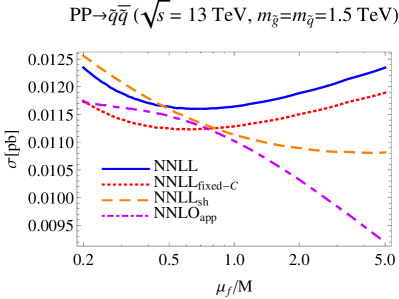
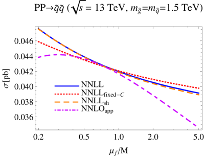
Refer to caption
Refer to caption
Refer to caption
Refer to caption
Figure 6: Cross section for squark and gluino production at the LHC with s=13𝑠13\sqrt{s}=13 TeV for full NNLL resummation (solid blue), NNLL with fixed-order Coulomb corrections (dotted red), NNLLshsubscriptNNLLsh\text{NNLL}_{\mathrm{sh}} (dashed orange) and approximate NNLO (dot-dashed pink), as a function of the ratio of the factorization scale and average produced mass.

The scale dependence of various higher-order approximations is shown in Figure 6. In addition to the approximate NNLO corrections, the full NNLL result and the NNLL soft resummation with fixed-order Coulomb corrections NNLLfixed-CsubscriptNNLLfixed-C\text{NNLL}_{\text{fixed-C}}, we also consider an approximation NNLLshsubscriptNNLLsh\text{NNLL}_{\text{sh}} where Coulomb corrections are set to zero in the resummation formula and only included through the matching to NNLOappsubscriptNNLOapp\text{NNLO}_{\text{app}}. It is seen that soft resummation in NNLLshsubscriptNNLLsh\text{NNLL}_{\text{sh}} significantly affects the shape of the scale dependence and reduces the scale uncertainty for squark-antisquark and squark-squark production. For the mass values considered here, the approximate NNLO cross section has a maximum near the default scale μf=Msubscript𝜇𝑓𝑀\mu_{f}=M, so the variation of the factorization scale alone leads to an asymmetrical error estimate, whereas the soft resummation leads to a more symmetrical behaviour. The inclusion of soft-Coulomb interference in the NNLLfixed-CsubscriptNNLLfixed-C\text{NNLL}_{\text{fixed-C}} prediction further reduces the uncertainty for the case of squark-antisquark and squark-squark production, while it is increased for gluino-pair and squark-gluino production. This observation is consistent with the results obtained in the Mellin-space approach for gluino-pair production [20]. The further resummation of Coulomb corrections in the NNLL prediction provides an overall shift of the cross section while the scale dependence is qualitatively similar to the NNLLfixed-CsubscriptNNLLfixed-C\text{NNLL}_{\text{fixed-C}} approximation.

mq~subscript𝑚~𝑞m_{\tilde{q}},mg~(TeV)subscript𝑚~𝑔TeVm_{\tilde{g}}(\mathrm{TeV}) s~s~~𝑠superscript~𝑠\tilde{s}\tilde{s}^{\prime} σNLL(pb)subscript𝜎NLLpb\sigma_{\mathrm{NLL}}(\mathrm{pb}) σNNLOapp(pb)subscript𝜎subscriptNNLOapppb\sigma_{\mathrm{NNLO}_{\mathrm{app}}}(\mathrm{pb}) σNNLLfixedC(pb)subscript𝜎subscriptNNLLfixedCpb\sigma_{\mathrm{NNLL}_{\mathrm{fixed-C}}}(\mathrm{pb}) σNNLL(pb)subscript𝜎NNLLpb\sigma_{\mathrm{NNLL}}(\mathrm{pb})
1.3,1.5 q~q~¯~𝑞¯~𝑞\tilde{q}\overline{\tilde{q}} 3.060.02+0.14×0.11+0.121023.06_{-0.02}^{+0.14}{}_{-0.11}^{+0.12}\times 10^{-2} 3.320.18+0.09×0.07+0.071023.32_{-0.18}^{+0.09}{}_{-0.07}^{+0.07}\times 10^{-2} 3.390.04+0.08×0.09+0.121023.39_{-0.04}^{+0.08}{}_{-0.09}^{+0.12}\times 10^{-2} 3.490.03+0.09×0.08+0.091023.49_{-0.03}^{+0.09}{}_{-0.08}^{+0.09}\times 10^{-2}
q~q~~𝑞~𝑞\tilde{q}\tilde{q} 8.760.55+0.75×0.07+0.091028.76_{-0.55}^{+0.75}{}_{-0.07}^{+0.09}\times 10^{-2} 9.310.53+0.31×0.46+0.461029.31_{-0.53}^{+0.31}{}_{-0.46}^{+0.46}\times 10^{-2} 9.380.19+0.21×0.46+0.481029.38_{-0.19}^{+0.21}{}_{-0.46}^{+0.48}\times 10^{-2} 9.370.25+0.32×0.47+0.461029.37_{-0.25}^{+0.32}{}_{-0.47}^{+0.46}\times 10^{-2}
q~g~~𝑞~𝑔\tilde{q}\tilde{g} 7.930.02+0.20×0.37+0.211027.93_{-0.02}^{+0.20}{}_{-0.37}^{+0.21}\times 10^{-2} 8.270.26+0.00×0.06+0.061028.27^{+0.00}_{-0.26}{}_{-0.06}^{+0.06}\times 10^{-2} 8.380.42+0.39×0.09+0.071028.38_{-0.42}^{+0.39}{}_{-0.09}^{+0.07}\times 10^{-2} 8.490.46+0.42×0.08+0.061028.49_{-0.46}^{+0.42}{}_{-0.08}^{+0.06}\times 10^{-2}
g~g~~𝑔~𝑔\tilde{g}\tilde{g} 8.030.32+0.55×0.58+0.591038.03_{-0.32}^{+0.55}{}_{-0.58}^{+0.59}\times 10^{-3} 7.970.25+0.00×0.41+0.411037.97^{+0.00}_{-0.25}{}_{-0.41}^{+0.41}\times 10^{-3} 8.140.61+0.55×0.42+0.411038.14_{-0.61}^{+0.55}{}_{-0.42}^{+0.41}\times 10^{-3} 8.710.77+0.69×0.44+0.441038.71_{-0.77}^{+0.69}{}_{-0.44}^{+0.44}\times 10^{-3}
1.5,1.3 q~q~¯~𝑞¯~𝑞\tilde{q}\overline{\tilde{q}} 1.020.01+0.05×0.04+0.041021.02_{-0.01}^{+0.05}{}_{-0.04}^{+0.04}\times 10^{-2} 1.110.07+0.04×0.04+0.041021.11_{-0.07}^{+0.04}{}_{-0.04}^{+0.04}\times 10^{-2} 1.130.01+0.02×0.04+0.051021.13_{-0.01}^{+0.02}{}_{-0.04}^{+0.05}\times 10^{-2} 1.170.01+0.02×0.04+0.041021.17_{-0.01}^{+0.02}{}_{-0.04}^{+0.04}\times 10^{-2}
q~q~~𝑞~𝑞\tilde{q}\tilde{q} 4.250.34+0.46×0.04+0.041024.25_{-0.34}^{+0.46}{}_{-0.04}^{+0.04}\times 10^{-2} 4.550.34+0.26×0.39+0.391024.55_{-0.34}^{+0.26}{}_{-0.39}^{+0.39}\times 10^{-2} 4.590.15+0.20×0.39+0.401024.59_{-0.15}^{+0.20}{}_{-0.39}^{+0.40}\times 10^{-2} 4.580.19+0.26×0.39+0.391024.58_{-0.19}^{+0.26}{}_{-0.39}^{+0.39}\times 10^{-2}
q~g~~𝑞~𝑔\tilde{q}\tilde{g} 9.590.00+0.23×0.47+0.271029.59^{+0.23}_{-0.00}{}_{-0.47}^{+0.27}\times 10^{-2} 1.020.03+0.00×0.02+0.021011.02^{+0.00}_{-0.03}{}_{-0.02}^{+0.02}\times 10^{-1} 1.050.05+0.05×0.03+0.031011.05_{-0.05}^{+0.05}{}_{-0.03}^{+0.03}\times 10^{-1} 1.060.05+0.06×0.03+0.021011.06_{-0.05}^{+0.06}{}_{-0.03}^{+0.02}\times 10^{-1}
g~g~~𝑔~𝑔\tilde{g}\tilde{g} 2.970.03+0.12×0.19+0.201022.97_{-0.03}^{+0.12}{}_{-0.19}^{+0.20}\times 10^{-2} 3.080.12+0.02×0.08+0.081023.08_{-0.12}^{+0.02}{}_{-0.08}^{+0.08}\times 10^{-2} 3.140.13+0.15×0.09+0.101023.14_{-0.13}^{+0.15}{}_{-0.09}^{+0.10}\times 10^{-2} 3.360.19+0.19×0.10+0.101023.36_{-0.19}^{+0.19}{}_{-0.10}^{+0.10}\times 10^{-2}
1.8,2 q~q~¯~𝑞¯~𝑞\tilde{q}\overline{\tilde{q}} 1.870.02+0.08×0.08+0.081031.87_{-0.02}^{+0.08}{}_{-0.08}^{+0.08}\times 10^{-3} 2.020.14+0.09×0.04+0.041032.02_{-0.14}^{+0.09}{}_{-0.04}^{+0.04}\times 10^{-3} 2.080.01+0.04×0.06+0.081032.08_{-0.01}^{+0.04}{}_{-0.06}^{+0.08}\times 10^{-3} 2.160.01+0.04×0.05+0.051032.16_{-0.01}^{+0.04}{}_{-0.05}^{+0.05}\times 10^{-3}
q~q~~𝑞~𝑞\tilde{q}\tilde{q} 9.820.67+0.91×0.13+0.121039.82_{-0.67}^{+0.91}{}_{-0.13}^{+0.12}\times 10^{-3} 1.050.07+0.05×0.05+0.051021.05_{-0.07}^{+0.05}{}_{-0.05}^{+0.05}\times 10^{-2} 1.060.02+0.03×0.06+0.061021.06_{-0.02}^{+0.03}{}_{-0.06}^{+0.06}\times 10^{-2} 1.060.03+0.04×0.06+0.051021.06_{-0.03}^{+0.04}{}_{-0.06}^{+0.05}\times 10^{-2}
q~g~~𝑞~𝑔\tilde{q}\tilde{g} 5.860.05+0.19×0.34+0.191035.86_{-0.05}^{+0.19}{}_{-0.34}^{+0.19}\times 10^{-3} 6.070.15+0.00×0.04+0.041036.07^{+0.00}_{-0.15}{}_{-0.04}^{+0.04}\times 10^{-3} 6.230.35+0.33×0.08+0.051036.23_{-0.35}^{+0.33}{}_{-0.08}^{+0.05}\times 10^{-3} 6.340.38+0.36×0.08+0.041036.34_{-0.38}^{+0.36}{}_{-0.08}^{+0.04}\times 10^{-3}
g~g~~𝑔~𝑔\tilde{g}\tilde{g} 4.330.27+0.38×0.37+0.361044.33_{-0.27}^{+0.38}{}_{-0.37}^{+0.36}\times 10^{-4} 4.140.16+0.00×0.23+0.231044.14^{+0.00}_{-0.16}{}_{-0.23}^{+0.23}\times 10^{-4} 4.350.38+0.35×0.23+0.231044.35_{-0.38}^{+0.35}{}_{-0.23}^{+0.23}\times 10^{-4} 4.710.48+0.43×0.24+0.251044.71_{-0.48}^{+0.43}{}_{-0.24}^{+0.25}\times 10^{-4}
2.,1.8 q~q~¯~𝑞¯~𝑞\tilde{q}\overline{\tilde{q}} 6.620.07+0.28×0.27+0.311046.62_{-0.07}^{+0.28}{}_{-0.27}^{+0.31}\times 10^{-4} 7.150.53+0.35×0.20+0.201047.15_{-0.53}^{+0.35}{}_{-0.20}^{+0.20}\times 10^{-4} 7.390.04+0.11×0.24+0.311047.39_{-0.04}^{+0.11}{}_{-0.24}^{+0.31}\times 10^{-4} 7.690.04+0.14×0.22+0.231047.69_{-0.04}^{+0.14}{}_{-0.22}^{+0.23}\times 10^{-4}
q~q~~𝑞~𝑞\tilde{q}\tilde{q} 4.780.39+0.53×0.07+0.051034.78_{-0.39}^{+0.53}{}_{-0.07}^{+0.05}\times 10^{-3} 5.160.42+0.32×0.40+0.401035.16_{-0.42}^{+0.32}{}_{-0.40}^{+0.40}\times 10^{-3} 5.240.17+0.22×0.40+0.411035.24_{-0.17}^{+0.22}{}_{-0.40}^{+0.41}\times 10^{-3} 5.230.21+0.28×0.40+0.401035.23_{-0.21}^{+0.28}{}_{-0.40}^{+0.40}\times 10^{-3}
q~g~~𝑞~𝑔\tilde{q}\tilde{g} 6.820.01+0.17×0.41+0.221036.82_{-0.01}^{+0.17}{}_{-0.41}^{+0.22}\times 10^{-3} 7.200.26+0.02×0.13+0.131037.20_{-0.26}^{+0.02}{}_{-0.13}^{+0.13}\times 10^{-3} 7.480.39+0.42×0.17+0.151037.48_{-0.39}^{+0.42}{}_{-0.17}^{+0.15}\times 10^{-3} 7.620.41+0.44×0.17+0.131037.62_{-0.41}^{+0.44}{}_{-0.17}^{+0.13}\times 10^{-3}
g~g~~𝑔~𝑔\tilde{g}\tilde{g} 1.400.03+0.08×0.11+0.111031.40_{-0.03}^{+0.08}{}_{-0.11}^{+0.11}\times 10^{-3} 1.410.08+0.01×0.04+0.041031.41_{-0.08}^{+0.01}{}_{-0.04}^{+0.04}\times 10^{-3} 1.470.08+0.09×0.05+0.051031.47_{-0.08}^{+0.09}{}_{-0.05}^{+0.05}\times 10^{-3} 1.600.12+0.12×0.05+0.051031.60_{-0.12}^{+0.12}{}_{-0.05}^{+0.05}\times 10^{-3}
2.3,2.5 q~q~¯~𝑞¯~𝑞\tilde{q}\overline{\tilde{q}} 1.320.01+0.06×0.06+0.071041.32_{-0.01}^{+0.06}{}_{-0.06}^{+0.07}\times 10^{-4} 1.410.12+0.09×0.03+0.031041.41_{-0.12}^{+0.09}{}_{-0.03}^{+0.03}\times 10^{-4} 1.480.01+0.02×0.04+0.061041.48_{-0.01}^{+0.02}{}_{-0.04}^{+0.06}\times 10^{-4} 1.550.01+0.03×0.03+0.041041.55_{-0.01}^{+0.03}{}_{-0.03}^{+0.04}\times 10^{-4}
q~q~~𝑞~𝑞\tilde{q}\tilde{q} 1.210.09+0.12×0.02+0.021031.21_{-0.09}^{+0.12}{}_{-0.02}^{+0.02}\times 10^{-3} 1.310.10+0.07×0.07+0.071031.31_{-0.10}^{+0.07}{}_{-0.07}^{+0.07}\times 10^{-3} 1.330.03+0.04×0.07+0.071031.33_{-0.03}^{+0.04}{}_{-0.07}^{+0.07}\times 10^{-3} 1.330.04+0.05×0.07+0.071031.33_{-0.04}^{+0.05}{}_{-0.07}^{+0.07}\times 10^{-3}
q~g~~𝑞~𝑔\tilde{q}\tilde{g} 5.130.08+0.23×0.36+0.191045.13_{-0.08}^{+0.23}{}_{-0.36}^{+0.19}\times 10^{-4} 5.230.19+0.00×0.03+0.031045.23^{+0.00}_{-0.19}{}_{-0.03}^{+0.03}\times 10^{-4} 5.490.35+0.34×0.09+0.041045.49_{-0.35}^{+0.34}{}_{-0.09}^{+0.04}\times 10^{-4} 5.600.38+0.37×0.09+0.041045.60_{-0.38}^{+0.37}{}_{-0.09}^{+0.04}\times 10^{-4}
g~g~~𝑔~𝑔\tilde{g}\tilde{g} 2.840.24+0.32×0.27+0.261052.84_{-0.24}^{+0.32}{}_{-0.27}^{+0.26}\times 10^{-5} 2.590.14+0.01×0.12+0.121052.59_{-0.14}^{+0.01}{}_{-0.12}^{+0.12}\times 10^{-5} 2.820.29+0.28×0.13+0.131052.82_{-0.29}^{+0.28}{}_{-0.13}^{+0.13}\times 10^{-5} 3.110.36+0.35×0.14+0.141053.11_{-0.36}^{+0.35}{}_{-0.14}^{+0.14}\times 10^{-5}
2.5,2.3 q~q~¯~𝑞¯~𝑞\tilde{q}\overline{\tilde{q}} 4.720.03+0.17×0.22+0.251054.72_{-0.03}^{+0.17}{}_{-0.22}^{+0.25}\times 10^{-5} 5.030.42+0.31×0.12+0.121055.03_{-0.42}^{+0.31}{}_{-0.12}^{+0.12}\times 10^{-5} 5.290.04+0.09×0.17+0.221055.29_{-0.04}^{+0.09}{}_{-0.17}^{+0.22}\times 10^{-5} 5.560.05+0.13×0.14+0.161055.56_{-0.05}^{+0.13}{}_{-0.14}^{+0.16}\times 10^{-5}
q~q~~𝑞~𝑞\tilde{q}\tilde{q} 5.740.47+0.65×0.11+0.081045.74_{-0.47}^{+0.65}{}_{-0.11}^{+0.08}\times 10^{-4} 6.220.55+0.44×0.44+0.441046.22_{-0.55}^{+0.44}{}_{-0.44}^{+0.44}\times 10^{-4} 6.380.20+0.27×0.45+0.461046.38_{-0.20}^{+0.27}{}_{-0.45}^{+0.46}\times 10^{-4} 6.360.24+0.34×0.45+0.441046.36_{-0.24}^{+0.34}{}_{-0.45}^{+0.44}\times 10^{-4}
q~g~~𝑞~𝑔\tilde{q}\tilde{g} 5.830.04+0.22×0.41+0.221045.83_{-0.04}^{+0.22}{}_{-0.41}^{+0.22}\times 10^{-4} 6.050.28+0.05×0.09+0.091046.05_{-0.28}^{+0.05}{}_{-0.09}^{+0.09}\times 10^{-4} 6.420.38+0.41×0.15+0.121046.42_{-0.38}^{+0.41}{}_{-0.15}^{+0.12}\times 10^{-4} 6.560.40+0.44×0.15+0.091046.56_{-0.40}^{+0.44}{}_{-0.15}^{+0.09}\times 10^{-4}
g~g~~𝑔~𝑔\tilde{g}\tilde{g} 8.620.39+0.72×0.76+0.741058.62_{-0.39}^{+0.72}{}_{-0.76}^{+0.74}\times 10^{-5} 8.380.56+0.19×0.24+0.241058.38_{-0.56}^{+0.19}{}_{-0.24}^{+0.24}\times 10^{-5} 9.070.65+0.71×0.27+0.301059.07_{-0.65}^{+0.71}{}_{-0.27}^{+0.30}\times 10^{-5} 1.000.09+0.09×0.03+0.031041.00_{-0.09}^{+0.09}{}_{-0.03}^{+0.03}\times 10^{-4}
2.8,3 q~q~¯~𝑞¯~𝑞\tilde{q}\overline{\tilde{q}} 9.690.03+0.32×0.47+0.541069.69_{-0.03}^{+0.32}{}_{-0.47}^{+0.54}\times 10^{-6} 1.020.09+0.07×0.02+0.021051.02_{-0.09}^{+0.07}{}_{-0.02}^{+0.02}\times 10^{-5} 1.090.01+0.02×0.03+0.041051.09_{-0.01}^{+0.02}{}_{-0.03}^{+0.04}\times 10^{-5} 1.150.01+0.03×0.02+0.031051.15_{-0.01}^{+0.03}{}_{-0.02}^{+0.03}\times 10^{-5}
q~q~~𝑞~𝑞\tilde{q}\tilde{q} 1.470.11+0.15×0.04+0.021041.47_{-0.11}^{+0.15}{}_{-0.04}^{+0.02}\times 10^{-4} 1.590.14+0.10×0.08+0.081041.59_{-0.14}^{+0.10}{}_{-0.08}^{+0.08}\times 10^{-4} 1.640.04+0.05×0.08+0.091041.64_{-0.04}^{+0.05}{}_{-0.08}^{+0.09}\times 10^{-4} 1.640.05+0.07×0.08+0.081041.64_{-0.05}^{+0.07}{}_{-0.08}^{+0.08}\times 10^{-4}
q~g~~𝑞~𝑔\tilde{q}\tilde{g} 4.620.14+0.25×0.38+0.201054.62_{-0.14}^{+0.25}{}_{-0.38}^{+0.20}\times 10^{-5} 4.610.24+0.03×0.03+0.031054.61_{-0.24}^{+0.03}{}_{-0.03}^{+0.03}\times 10^{-5} 4.970.36+0.34×0.10+0.041054.97_{-0.36}^{+0.34}{}_{-0.10}^{+0.04}\times 10^{-5} 5.100.39+0.37×0.10+0.031055.10_{-0.39}^{+0.37}{}_{-0.10}^{+0.03}\times 10^{-5}
g~g~~𝑔~𝑔\tilde{g}\tilde{g} 1.970.22+0.26×0.22+0.201061.97_{-0.22}^{+0.26}{}_{-0.22}^{+0.20}\times 10^{-6} 1.680.13+0.02×0.08+0.081061.68_{-0.13}^{+0.02}{}_{-0.08}^{+0.08}\times 10^{-6} 1.930.23+0.22×0.09+0.081061.93_{-0.23}^{+0.22}{}_{-0.09}^{+0.08}\times 10^{-6} 2.180.30+0.27×0.09+0.101062.18_{-0.30}^{+0.27}{}_{-0.09}^{+0.10}\times 10^{-6}
3.,2.8 q~q~¯~𝑞¯~𝑞\tilde{q}\overline{\tilde{q}} 3.500.01+0.09×0.17+0.201063.50_{-0.01}^{+0.09}{}_{-0.17}^{+0.20}\times 10^{-6} 3.680.34+0.25×0.08+0.081063.68_{-0.34}^{+0.25}{}_{-0.08}^{+0.08}\times 10^{-6} 3.930.05+0.08×0.12+0.171063.93_{-0.05}^{+0.08}{}_{-0.12}^{+0.17}\times 10^{-6} 4.170.07+0.10×0.10+0.111064.17_{-0.07}^{+0.10}{}_{-0.10}^{+0.11}\times 10^{-6}
q~q~~𝑞~𝑞\tilde{q}\tilde{q} 6.610.54+0.76×0.16+0.111056.61_{-0.54}^{+0.76}{}_{-0.16}^{+0.11}\times 10^{-5} 7.190.70+0.58×0.47+0.471057.19_{-0.70}^{+0.58}{}_{-0.47}^{+0.47}\times 10^{-5} 7.450.23+0.31×0.48+0.501057.45_{-0.23}^{+0.31}{}_{-0.48}^{+0.50}\times 10^{-5} 7.430.28+0.39×0.48+0.481057.43_{-0.28}^{+0.39}{}_{-0.48}^{+0.48}\times 10^{-5}
q~g~~𝑞~𝑔\tilde{q}\tilde{g} 5.160.09+0.25×0.42+0.231055.16_{-0.09}^{+0.25}{}_{-0.42}^{+0.23}\times 10^{-5} 5.240.32+0.07×0.07+0.071055.24_{-0.32}^{+0.07}{}_{-0.07}^{+0.07}\times 10^{-5} 5.710.39+0.40×0.14+0.101055.71_{-0.39}^{+0.40}{}_{-0.14}^{+0.10}\times 10^{-5} 5.870.42+0.43×0.14+0.071055.87_{-0.42}^{+0.43}{}_{-0.14}^{+0.07}\times 10^{-5}
g~g~~𝑔~𝑔\tilde{g}\tilde{g} 5.900.42+0.63×0.60+0.571065.90_{-0.42}^{+0.63}{}_{-0.60}^{+0.57}\times 10^{-6} 5.430.46+0.20×0.16+0.161065.43_{-0.46}^{+0.20}{}_{-0.16}^{+0.16}\times 10^{-6} 6.160.56+0.58×0.19+0.211066.16_{-0.56}^{+0.58}{}_{-0.19}^{+0.21}\times 10^{-6} 6.940.73+0.75×0.20+0.211066.94_{-0.73}^{+0.75}{}_{-0.20}^{+0.21}\times 10^{-6}
Table 7: Different higher-order approximations for the LHC with s=13𝑠13\sqrt{s}=13 TeV. The first error denotes the scale variation while the second error refers to the estimate of the remaining theoretical uncertainty. The latter is given by the resummation uncertainty (NLL), the variation of the two-loop constant (NNLOappapp{}_{\text{app}}), while for the two NNLL results the two errors are added in quadrature.

In Table 7 we provide numerical results for the higher-order approximations NLL, NLLOappapp{}_{\text{app}}, NNLLfixed-C and NNLL defined above. In order to study the contributions of the different sources of uncertainties, the scale uncertainty is shown separately from the remaining theoretical uncertainties. The results are shown for the same mass values as in Table 5. The magnitude of the corrections from the successive improvement in accuracy is consistent with that seen in Figure 3. The difference between the approximate NNLO results and the resummed predictions is moderate at smaller masses but grows more sizeable for heavy sparticles. The higher-order Coulomb corrections and bound-state effects only included in the full NNLL results become important in particular for squark-antisquark and gluino-pair production at high masses, whereas the corrections are moderate for squark-gluino production and small for squark-squark production. The uncertainty from resummation ambiguities and missing higher-order corrections is strongly reduced from NLL to NNLL for all processes with the exception of squark-squark production. It is seen that this uncertainty is dominated by the two-loop constant variation, which is identical for NNLOappapp{}_{\text{app}} and the two NNLL implementations. The scale uncertainty alone is usually reduced for the NNLOappapp{}_{\text{app}} approximation, but can be very asymmetric as seen already in Figure 6. For a more realistic uncertainty estimate at this order, the renormalization scale should be varied independently. The scale uncertainty is further reduced at NNLL for squark-antisquark and squark-squark production but increased for squark-gluino and gluino-pair production, consistent with Figure 5.

4 Conclusions

We performed a combined NNLL resummation of soft-gluon and Coulomb corrections for all squark- and gluino-pair production channels at the LHC based on the method developed for top-quark pair production [51], extending an earlier NLL study [16]. Grids with our NNLL predictions for the LHC with s=13𝑠13\sqrt{s}=13 and 141414 TeV for mq~,mg~=200subscript𝑚~𝑞subscript𝑚~𝑔200m_{\tilde{q}},m_{\tilde{g}}=200300030003000 GeV and 200200200350035003500 GeV, respectively, are publicly available [1]. We furthermore completed the result for the NNLO threshold expansion of the total cross section [53] by deriving the spin-dependent non-Coulomb corrections and the process-specific annihilation contributions, which both give rise to a single-logarithmic NNLO correction.

Our NNLL results show generally moderate corrections to the NLL predictions with combined soft-Coulomb corrections [16], which shows that the combined resummation is the adequate method to control the QCD corrections in the region of large sparticle masses, where both the NLO SQCD and the NLL soft-gluon and Coulomb corrections can become very large, especially for gluino-pair production. Corrections beyond NNLO included in the resummed results become sizeable for sparticle masses above 1.5TeV1.5TeV1.5\,\mathrm{TeV}. We carefully estimated uncertainties due to scale choices and ambiguities of the resummation formalism and found that the total theoretical uncertainty of the squark and gluino pair production processes due to missing higher-order corrections is reduced to the 10%percent1010\% level. We also compared different scale-setting procedures for the soft scale in the momentum-space formalism for soft-gluon resummation and found a better agreement compared to the NLL calculation. The NNLL calculation leaves the PDF uncertainties as the dominant source of uncertainties, which can hopefully be reduced in the future using constraints from measurements at the LHC.

Note added:

In the final stages of this work we became aware of related work on the combined soft-Coulomb resummation in the Mellin-space formalism [83], where a detailed comparison to our results from [19] is performed.

Acknowledgements

We would like to thank Pietro Falgari for collaboration in the early stages of this work, Anna Kulesza for correspondence on the hard matching coefficients computed in [59] and Michael Krämer for sharing a draft of [83]. The work of MB is supported by the BMBF grant 05H15WOCAA. The work of CW was partially funded by Research Funding Program ARISTEIA, HOCTools (co-financed by the European Union (European Social Fund ESF) and Greek national funds through the Operational Program ”Education and Lifelong Learning” of the National Strategic Reference Framework (NSRF)). CS is supported by the Heisenberg Programme of the DFG. JP and CS acknowledge support by the Munich Institute for Astro- and Particle Physics (MIAPP) of the DFG cluster of excellence ”Origin and Structure of the Universe” and the Mainz Institute for Theoretical Physics (MITP) during parts of this work.

Appendix A Explicit formulae

A.1 Expansion of the NNLL cross section

In this appendix we collect the expansions of the NNLL correction factors to 𝒪(αs)𝒪subscript𝛼𝑠\mathcal{O}(\alpha_{s}) and 𝒪(αs2)𝒪superscriptsubscript𝛼𝑠2\mathcal{O}(\alpha_{s}^{2}), respectively. The expansion to NLO accuracy yields all threshold-enhanced NLO terms and the constant term,

fpp,iNNLL(1)subscriptsuperscript𝑓NNLL1𝑝superscript𝑝𝑖\displaystyle f^{\mathrm{NNLL}(1)}_{pp^{\prime},i} =\displaystyle= 2π2DRαβ2mrM+4Crr[LE2+6ln2LE]2superscript𝜋2subscript𝐷subscript𝑅𝛼𝛽2subscript𝑚𝑟𝑀4subscript𝐶𝑟superscript𝑟delimited-[]subscriptsuperscriptL2𝐸62subscriptL𝐸\displaystyle-\frac{2\pi^{2}D_{R_{\alpha}}}{\beta}\sqrt{\frac{2m_{r}}{M}}+4C_{rr^{\prime}}\left[\mathrm{L}^{2}_{E}+6\ln 2\,\mathrm{L}_{E}\right] (A.1)
4(CRα+4Crr)LE+Cpp,i(1)(μ)+𝒪(β).4subscript𝐶subscript𝑅𝛼4subscript𝐶𝑟superscript𝑟subscriptL𝐸subscriptsuperscript𝐶1𝑝superscript𝑝𝑖𝜇𝒪𝛽\displaystyle-4(C_{R_{\alpha}}+4C_{rr^{\prime}})\mathrm{L}_{E}+C^{(1)}_{pp^{\prime},i}(\mu)+{\cal O}(\beta).

Here and in the following we use the notation

Lx=ln(xμf),subscriptL𝑥𝑥subscript𝜇𝑓\mathrm{L}_{x}=\ln\left(\frac{x}{\mu_{f}}\right)\;, (A.2)

and the sum of the two quadratic Casimir operators of the colour representation of the incoming partons has been defined as

Crr=Cr+Cr.subscript𝐶𝑟superscript𝑟subscript𝐶𝑟subscript𝐶superscript𝑟C_{rr^{\prime}}=C_{r}+C_{r^{\prime}}. (A.3)

The constant term can be expressed in terms of the one-loop hard coefficient in (2.12) by the relation

Cpp,i(1)(μ)=hi(1)(μ)+4Crr[9ln2212ln2+811π224]12CR[ln21].subscriptsuperscript𝐶1𝑝superscript𝑝𝑖𝜇subscriptsuperscript1𝑖𝜇4subscript𝐶𝑟superscript𝑟delimited-[]9superscript22122811superscript𝜋22412subscript𝐶𝑅delimited-[]21C^{(1)}_{pp^{\prime},i}(\mu)=h^{(1)}_{i}(\mu)+4\,C_{rr^{\prime}}\bigg{[}9\ln^{2}2-12\ln 2+8-\frac{11\pi^{2}}{24}\bigg{]}-12C_{R}\left[\ln 2-1\right]\,. (A.4)

The expansion to NNLO accuracy reads777In the corresponding formula in the journal version of this paper we have set CA=3subscript𝐶𝐴3C_{A}=3.

fpp,iNNLL(2)=subscriptsuperscript𝑓NNLL2𝑝superscript𝑝𝑖absent\displaystyle f^{\mathrm{NNLL}(2)}_{pp^{\prime},i}= 4π4DRα23β22mredM+2π2DRαβ2mredM{4Crr(L2E2+Lμh(Lμh2L2M)π28)\displaystyle\frac{4\pi^{4}D_{R_{\alpha}}^{2}}{3\beta^{2}}\frac{2m_{\mathrm{red}}}{M}+\frac{2\pi^{2}D_{R_{\alpha}}}{\beta}\sqrt{\frac{2m_{\mathrm{red}}}{M}}\Biggl{\{}-4C_{rr^{\prime}}\left(\mathrm{L}^{2}_{2E}+\mathrm{L}_{\mu_{h}}(\mathrm{L}_{\mu_{h}}-2\mathrm{L}_{2M})-\frac{\pi^{2}}{8}\right)
+L2E(β0+4CRα)2Lμh(2CRα+γrr(0)2β0)+β0L4mredsubscriptL2𝐸subscript𝛽04subscript𝐶subscript𝑅𝛼2subscriptLsubscript𝜇2subscript𝐶subscript𝑅𝛼superscriptsubscript𝛾𝑟superscript𝑟02subscript𝛽0subscript𝛽0subscriptL4subscript𝑚red\displaystyle+\mathrm{L}_{2E}(\beta_{0}+4C_{R_{\alpha}})-2\mathrm{L}_{\mu_{h}}\left(2C_{R_{\alpha}}+\gamma_{rr^{\prime}}^{(0)}-2\beta_{0}\right)+\beta_{0}\mathrm{L}_{4m_{\mathrm{red}}}
a14CRαh1(i)(μh)}\displaystyle-a_{1}-4C_{R_{\alpha}}-h_{1}^{(i)}(\mu_{h})\Biggr{\}}
+8π2DRα(CA2DRα(1+νspinS)124mred2M2νannRα,S)lnEM8superscript𝜋2subscript𝐷subscript𝑅𝛼subscript𝐶𝐴2subscript𝐷subscript𝑅𝛼1superscriptsubscript𝜈spin𝑆124superscriptsubscript𝑚red2superscript𝑀2superscriptsubscript𝜈annsubscript𝑅𝛼𝑆𝐸𝑀\displaystyle+8\pi^{2}D_{R_{\alpha}}\left(C_{A}-2D_{R_{\alpha}}(1+\nu_{\mathrm{spin}}^{S})-\frac{1}{2}\frac{4m_{\mathrm{red}}^{2}}{M^{2}}\nu_{\mathrm{ann}}^{R_{\alpha},S}\right)\ln\frac{E}{M}
+8Crr2(L8E4L8Es4+Lμh4)16Crr(β06+4Crr+CRα)(L8E3L8Es3)8superscriptsubscript𝐶𝑟superscript𝑟2subscriptsuperscriptL48𝐸subscriptsuperscriptL48subscript𝐸𝑠subscriptsuperscriptL4subscript𝜇16subscript𝐶𝑟superscript𝑟subscript𝛽064subscript𝐶𝑟superscript𝑟subscript𝐶subscript𝑅𝛼subscriptsuperscriptL38𝐸subscriptsuperscriptL38subscript𝐸𝑠\displaystyle+8C_{rr^{\prime}}^{2}\left(\mathrm{L}^{4}_{8E}-\mathrm{L}^{4}_{8E_{s}}+\mathrm{L}^{4}_{\mu_{h}}\right)-16C_{rr^{\prime}}\left(\frac{\beta_{0}}{6}+4C_{rr^{\prime}}+C_{R_{\alpha}}\right)\left(\mathrm{L}^{3}_{8E}-\mathrm{L}^{3}_{8E_{s}}\right)
8Crr[4CrrL2M+8β03γrr(0)2CRα]Lμh38subscript𝐶𝑟superscript𝑟delimited-[]4subscript𝐶𝑟superscript𝑟subscriptL2𝑀8subscript𝛽03superscriptsubscript𝛾𝑟superscript𝑟02subscript𝐶subscript𝑅𝛼subscriptsuperscriptL3subscript𝜇\displaystyle-8C_{rr^{\prime}}\Bigl{[}4C_{rr^{\prime}}\mathrm{L}_{2M}+\frac{8\beta_{0}}{3}-\gamma_{rr^{\prime}}^{(0)}-2C_{R_{\alpha}}\Bigr{]}\mathrm{L}^{3}_{\mu_{h}}
+{Crr2(38470π23)+4Crr[4β0+28CRα+CA(679π23)20nfTF9]\displaystyle+\Biggl{\{}C_{rr^{\prime}}^{2}\left(384-\frac{70\pi^{2}}{3}\right)+4C_{rr^{\prime}}\left[4\beta_{0}+28C_{R_{\alpha}}+C_{A}\left(\frac{67}{9}-\frac{\pi^{2}}{3}\right)-\frac{20n_{f}T_{F}}{9}\right]
+4CRα(β0+2CRα)}(L8E2L8Es2)\displaystyle+4C_{R_{\alpha}}(\beta_{0}+2C_{R_{\alpha}})\Biggr{\}}\left(\mathrm{L}^{2}_{8E}-\mathrm{L}^{2}_{8E_{s}}\right)
+{16Crr2(L8E24L8E+2L2M211π224+8)\displaystyle+\Biggl{\{}16C_{rr^{\prime}}^{2}\left(\mathrm{L}^{2}_{8E}-4\mathrm{L}_{8E}+2\mathrm{L}^{2}_{2M}-\frac{11\pi^{2}}{24}+8\right)
+Crr[16CRαL8E+48CRα80nfTF94CA(π23679)\displaystyle+C_{rr^{\prime}}\Bigl{[}-16C_{R_{\alpha}}\mathrm{L}_{8E}+48C_{R_{\alpha}}-\frac{80n_{f}T_{F}}{9}-4C_{A}\left(\frac{\pi^{2}}{3}-\frac{67}{9}\right)
+(40β016γrr(0)32CRα)L2M]\displaystyle+\left(40\beta_{0}-16\gamma_{rr^{\prime}}^{(0)}-32C_{R_{\alpha}}\right)\mathrm{L}_{2M}\Bigr{]}
+12β0210β0(γrr(0)+2CRα)+2(γrr(0)+2CRα)2}L2μh\displaystyle+12\beta_{0}^{2}-10\beta_{0}(\gamma_{rr^{\prime}}^{(0)}+2C_{R_{\alpha}})+2(\gamma_{rr^{\prime}}^{(0)}+2C_{R_{\alpha}})^{2}\Biggr{\}}\,\mathrm{L}^{2}_{\mu_{h}}
+{Crr2(448ζ(3)1536+280π23)+Crr[(11π2364)β0\displaystyle+\Biggl{\{}C_{rr^{\prime}}^{2}\left(448\zeta(3)-1536+\frac{280\pi^{2}}{3}\right)+C_{rr^{\prime}}\Biggl{[}\left(\frac{11\pi^{2}}{3}-64\right)\beta_{0}
+(70π23448)CRα+CA(28ζ(3)+59π29402427)+nfTF(1184274π29)]\displaystyle+\left(\frac{70\pi^{2}}{3}-448\right)C_{R_{\alpha}}+C_{A}\left(28\zeta(3)+\frac{59\pi^{2}}{9}-\frac{4024}{27}\right)+n_{f}T_{F}\left(\frac{1184}{27}-\frac{4\pi^{2}}{9}\right)\Biggr{]}
+CRα[24β0+CA(8ζ(3)+4π231969)+80nfTF9]48CRα2}(L8EL8Es)\displaystyle+C_{R_{\alpha}}\left[-24\beta_{0}+C_{A}\left(-8\zeta(3)+\frac{4\pi^{2}}{3}-\frac{196}{9}\right)+\frac{80n_{f}T_{F}}{9}\right]-48C_{R_{\alpha}}^{2}\Biggr{\}}\,\left(\mathrm{L}_{8E}-\mathrm{L}_{8E_{s}}\right)
+{4Crr(L8E24L8E+Lμh211π224+8)\displaystyle+\Biggl{\{}4C_{rr^{\prime}}\left(\mathrm{L}^{2}_{8E}-4\mathrm{L}_{8E}+\mathrm{L}^{2}_{\mu_{h}}-\frac{11\pi^{2}}{24}+8\right)
4CRα(L8E3)2Lμh[4CrrL2M2CRα+3β0γrr(0)]}h1(i)(μh)\displaystyle-4C_{R_{\alpha}}\left(\mathrm{L}_{8E}-3\right)-2\mathrm{L}_{\mu_{h}}\Bigl{[}4C_{rr^{\prime}}\mathrm{L}_{2M}-2C_{R_{\alpha}}+3\beta_{0}-\gamma_{rr^{\prime}}^{(0)}\Bigr{]}\Biggr{\}}\,h_{1}^{(i)}(\mu_{h})
+{(4CrrL2M+2β0γrr(0)2CRα)[8CrrL8E2+8(4Crr+CRα)L8E\displaystyle+\Biggl{\{}\left(4C_{rr^{\prime}}\mathrm{L}_{2M}+2\beta_{0}-\gamma_{rr^{\prime}}^{(0)}-2C_{R_{\alpha}}\right)\Biggl{[}-8C_{rr^{\prime}}\mathrm{L}^{2}_{8E}+8(4C_{rr^{\prime}}+C_{R_{\alpha}})\mathrm{L}_{8E}
+Crr(64+11π23)24CRα]Crr[CA(53698π23)160nfTF9]L2M\displaystyle+C_{rr^{\prime}}\left(-64+\frac{11\pi^{2}}{3}\right)-24C_{R_{\alpha}}\Biggr{]}-C_{rr^{\prime}}\left[C_{A}\left(\frac{536}{9}-\frac{8\pi^{2}}{3}\right)-\frac{160n_{f}T_{F}}{9}\right]\mathrm{L}_{2M}
+Crr[CA(8082711π2928ζ(3))(224274π29)nfTF]subscript𝐶𝑟superscript𝑟delimited-[]subscript𝐶𝐴8082711superscript𝜋2928𝜁3224274superscript𝜋29subscript𝑛𝑓subscript𝑇𝐹\displaystyle+C_{rr^{\prime}}\left[C_{A}\left(\frac{808}{27}-\frac{11\pi^{2}}{9}-28\zeta(3)\right)-\left(\frac{224}{27}-\frac{4\pi^{2}}{9}\right)n_{f}T_{F}\right]
+2γrr(1)+CRα[CA(8ζ(3)+19694π23)80nfTF9]4β1}Lμh+Cpp,i(2).\displaystyle+2\gamma_{rr^{\prime}}^{(1)}+C_{R_{\alpha}}\left[C_{A}\left(8\zeta(3)+\frac{196}{9}-\frac{4\pi^{2}}{3}\right)-\frac{-80n_{f}T_{F}}{9}\right]-4\beta_{1}\Biggr{\}}\,\mathrm{L}_{\mu_{h}}+C_{pp^{\prime},i}^{(2)}. (A.5)

Here we further defined L8Es=ln(8Eμs)subscriptL8subscript𝐸𝑠8𝐸subscript𝜇𝑠\mathrm{L}_{8E_{s}}=\ln\left(\frac{8E}{\mu_{s}}\right). The two-loop beta-function coefficient is given by β1=343CA2203CATFnf4CFTFnfsubscript𝛽1343superscriptsubscript𝐶𝐴2203subscript𝐶𝐴subscript𝑇𝐹subscript𝑛𝑓4subscript𝐶𝐹subscript𝑇𝐹subscript𝑛𝑓\beta_{1}=\frac{34}{3}C_{A}^{2}-\frac{20}{3}C_{A}T_{F}n_{f}-4C_{F}T_{F}n_{f}. The anomalous-dimension coefficients appearing in this formula are related to the incoming partons and are defined as

γrr(n)=γϕ,r(n)+γϕ,r(n),superscriptsubscript𝛾𝑟superscript𝑟𝑛superscript𝛾italic-ϕ𝑟𝑛superscript𝛾italic-ϕsuperscript𝑟𝑛\gamma_{rr^{\prime}}^{(n)}=\gamma^{\phi,r(n)}+\gamma^{\phi,r^{\prime}(n)}, (A.6)

with

γϕ,3(0)superscript𝛾italic-ϕ30\displaystyle\gamma^{\phi,3(0)} =\displaystyle= 3CF,3subscript𝐶𝐹\displaystyle 3C_{F}, (A.7)
γϕ,3(1)superscript𝛾italic-ϕ31\displaystyle\gamma^{\phi,3(1)} =\displaystyle= CF2(322π2+24ζ3)+CACF(176+22π2912ζ3)superscriptsubscript𝐶𝐹2322superscript𝜋224subscript𝜁3subscript𝐶𝐴subscript𝐶𝐹17622superscript𝜋2912subscript𝜁3\displaystyle C_{F}^{2}\left(\frac{3}{2}-2\pi^{2}+24\zeta_{3}\right)+C_{A}C_{F}\left(\frac{17}{6}+\frac{22\pi^{2}}{9}-12\zeta_{3}\right) (A.8)
CFTFnf(23+8π29),subscript𝐶𝐹subscript𝑇𝐹subscript𝑛𝑓238superscript𝜋29\displaystyle-\,C_{F}T_{F}n_{f}\left(\frac{2}{3}+\frac{8\pi^{2}}{9}\right),
γϕ,8(0)superscript𝛾italic-ϕ80\displaystyle\gamma^{\phi,8(0)} =\displaystyle= β0=113CA43TFnf,subscript𝛽0113subscript𝐶𝐴43subscript𝑇𝐹subscript𝑛𝑓\displaystyle\beta_{0}=\frac{11}{3}C_{A}-\frac{4}{3}T_{F}n_{f}, (A.9)
γϕ,8(1)superscript𝛾italic-ϕ81\displaystyle\gamma^{\phi,8(1)} =\displaystyle= 4CA2(83+3ζ3)163CATFnf4CFTFnf.4superscriptsubscript𝐶𝐴2833subscript𝜁3163subscript𝐶𝐴subscript𝑇𝐹subscript𝑛𝑓4subscript𝐶𝐹subscript𝑇𝐹subscript𝑛𝑓\displaystyle 4C_{A}^{2}\left(\frac{8}{3}+3\zeta_{3}\right)-\frac{16}{3}C_{A}T_{F}n_{f}-4C_{F}T_{F}n_{f}. (A.10)

A.2 Analytic NNLL result for fixed-order Coulomb corrections

If the Coulomb corrections are treated at fixed NNLO accuracy through the factor (2.52), the ω𝜔\omega-convolution in the resummed cross section (2.10) can be performed explicitly, resulting in an analytic expression:

σ^ppres(s^,μ)=subscriptsuperscript^𝜎res𝑝superscript𝑝^𝑠𝜇absent\displaystyle\hat{\sigma}^{\text{res}}_{pp^{\prime}}(\hat{s},\mu)= iσpp,i(0)(μ)URα(μh,μs,μf)(2Mμs)2ηs~iRα(η,μs)𝒞hCNNLO(E,μh,μs,μf),subscript𝑖subscriptsuperscript𝜎0𝑝superscript𝑝𝑖𝜇subscript𝑈subscript𝑅𝛼subscript𝜇subscript𝜇𝑠subscript𝜇𝑓superscript2𝑀subscript𝜇𝑠2𝜂superscriptsubscript~𝑠𝑖subscript𝑅𝛼subscript𝜂subscript𝜇𝑠superscriptsubscript𝒞hCNNLO𝐸subscript𝜇subscript𝜇𝑠subscript𝜇𝑓\displaystyle\sum_{i}\sigma^{(0)}_{pp^{\prime},i}(\mu)U_{R_{\alpha}}(\mu_{h},\mu_{s},\mu_{f})\left(\frac{2M}{\mu_{s}}\right)^{-2\eta}\tilde{s}_{i}^{R_{\alpha}}(\partial_{\eta},\mu_{s})\,\mathcal{C}_{\text{hC}}^{\text{NNLO}}(E,\mu_{h},\mu_{s},\mu_{f}), (A.11)

with the Laplace transform of the NLO soft function (2.11) and where the function 𝒞hCNNLOsuperscriptsubscript𝒞hCNNLO\mathcal{C}_{\text{hC}}^{\text{NNLO}} is given by

𝒞hCNNLO(E,μh,μs,μf)superscriptsubscript𝒞hCNNLO𝐸subscript𝜇subscript𝜇𝑠subscript𝜇𝑓\displaystyle\mathcal{C}_{\text{hC}}^{\text{NNLO}}(E,\mu_{h},\mu_{s},\mu_{f}) =(2EeγEμs)2ηn=02(αs4π)n𝒞hC(n)(E,μh,μs,μf),absentsuperscript2𝐸superscript𝑒subscript𝛾𝐸subscript𝜇𝑠2𝜂superscriptsubscript𝑛02superscriptsubscript𝛼𝑠4𝜋𝑛superscriptsubscript𝒞hC𝑛𝐸subscript𝜇subscript𝜇𝑠subscript𝜇𝑓\displaystyle=\left(\frac{2Ee^{-\gamma_{E}}}{\mu_{s}}\right)^{2\eta}\sum_{n=0}^{2}\left(\frac{\alpha_{s}}{4\pi}\right)^{n}\mathcal{C}_{\text{hC}}^{(n)}(E,\mu_{h},\mu_{s},\mu_{f}), (A.12)
𝒞hC(0)(E,μh,μs,μf)superscriptsubscript𝒞hC0𝐸subscript𝜇subscript𝜇𝑠subscript𝜇𝑓\displaystyle\mathcal{C}_{\text{hC}}^{(0)}(E,\mu_{h},\mu_{s},\mu_{f}) =π2Γ(2η+32),absent𝜋2Γ2𝜂32\displaystyle=\frac{\sqrt{\pi}}{2\Gamma(2\eta+\frac{3}{2})}, (A.13)
𝒞hC(1)(E,μh,μs,μf)=superscriptsubscript𝒞hC1𝐸subscript𝜇subscript𝜇𝑠subscript𝜇𝑓absent\displaystyle\mathcal{C}_{\text{hC}}^{(1)}(E,\mu_{h},\mu_{s},\mu_{f})= (2π2DRα)Γ(2η+1)2mredE+π2Γ(2η+32)hi(1)(μh),2superscript𝜋2subscript𝐷subscript𝑅𝛼Γ2𝜂12subscript𝑚red𝐸𝜋2Γ2𝜂32subscriptsuperscript1𝑖subscript𝜇\displaystyle-\frac{(2\pi^{2}D_{R_{\alpha}})}{\Gamma(2\eta+1)}\sqrt{\frac{2m_{\mathrm{red}}}{E}}+\frac{\sqrt{\pi}}{2\Gamma(2\eta+\frac{3}{2})}\,h^{(1)}_{i}(\mu_{h}), (A.14)
𝒞hC(2)(E,μh,μs,μf)=superscriptsubscript𝒞hC2𝐸subscript𝜇subscript𝜇𝑠subscript𝜇𝑓absent\displaystyle\mathcal{C}_{\text{hC}}^{(2)}(E,\mu_{h},\mu_{s},\mu_{f})= π(2π2DRα)23Γ(2η+12)(2mredE)(2π2DRα)Γ(2η+1)2mredE𝜋superscript2superscript𝜋2subscript𝐷subscript𝑅𝛼23Γ2𝜂122subscript𝑚red𝐸2superscript𝜋2subscript𝐷subscript𝑅𝛼Γ2𝜂12subscript𝑚red𝐸\displaystyle\frac{\sqrt{\pi}(2\pi^{2}D_{R_{\alpha}})^{2}}{3\Gamma(2\eta+\frac{1}{2})}\left(\frac{2m_{\mathrm{red}}}{E}\right)-\frac{(2\pi^{2}D_{R_{\alpha}})}{\Gamma(2\eta+1)}\sqrt{\frac{2m_{\mathrm{red}}}{E}}
×[h1(i)(μh)+a1β0(ln(8Emredμ2)ψ(0)(2η+1)γE)]absentdelimited-[]superscriptsubscript1𝑖subscript𝜇subscript𝑎1subscript𝛽08𝐸subscript𝑚redsuperscript𝜇2superscript𝜓02𝜂1subscript𝛾𝐸\displaystyle\times\left[h_{1}^{(i)}(\mu_{h})+a_{1}-\beta_{0}\left(\ln\left(\frac{8Em_{\mathrm{red}}}{\mu^{2}}\right)-\psi^{(0)}(2\eta+1)-\gamma_{E}\right)\right]
+2π(2π2DRα)Γ(2η+32)(CA2DRα(vspin+1)νannRα,S24mred2M2)2𝜋2superscript𝜋2subscript𝐷subscript𝑅𝛼Γ2𝜂32subscript𝐶𝐴2subscript𝐷subscript𝑅𝛼subscript𝑣spin1superscriptsubscript𝜈annsubscript𝑅𝛼𝑆24superscriptsubscript𝑚red2superscript𝑀2\displaystyle+\frac{2\sqrt{\pi}(2\pi^{2}D_{R_{\alpha}})}{\Gamma(2\eta+\frac{3}{2})}\left(C_{A}-2D_{R_{\alpha}}(v_{\text{spin}}+1)-\frac{\nu_{\mathrm{ann}}^{R_{\alpha},S}}{2}\frac{4m_{\mathrm{red}}^{2}}{M^{2}}\right)
×(ln(EM)ψ(0)(2η+32)γE+22ln2)absent𝐸𝑀superscript𝜓02𝜂32subscript𝛾𝐸222\displaystyle\times\left(\ln\left(\frac{E}{M}\right)-\psi^{(0)}\left(2\eta+\frac{3}{2}\right)-\gamma_{E}+2-2\ln 2\right)
+π2Γ(2η+32)hi(1)(μh)(2β0)ln(μhμf),𝜋2Γ2𝜂32subscriptsuperscript1𝑖subscript𝜇2subscript𝛽0subscript𝜇subscript𝜇𝑓\displaystyle+\frac{\sqrt{\pi}}{2\Gamma(2\eta+\frac{3}{2})}\,h^{(1)}_{i}(\mu_{h})\,(-2\beta_{0})\ln\left(\frac{\mu_{h}}{\mu_{f}}\right), (A.15)

with the digamma function ψ(0)(x)=dlnΓ(x)dxsuperscript𝜓0𝑥𝑑Γ𝑥𝑑𝑥\psi^{(0)}(x)=\frac{d\ln\Gamma(x)}{dx}. It is straightforward to evaluate the action of the derivative with respect to η𝜂\eta in (A.11) on the factors (A.13)–(A.15).

References

  • [1] http://users.ph.tum.de/t31software/SUSYNNLL/.
  • [2] ATLAS Collaboration Collaboration, G. Aad et al., arXiv:1405.7875 [hep-ex].
  • [3] CMS Collaboration, V. Khachatryan et al., JHEP 05 (2015) 078, arXiv:1502.04358 [hep-ex].
  • [4] CMS Collaboration, V. Khachatryan et al., arXiv:1603.04053 [hep-ex].
  • [5] W. Beenakker, R. Höpker, M. Spira, and P. M. Zerwas, Nucl. Phys. B492 (1997) 51–103, arXiv:hep-ph/9610490.
  • [6] W. Beenakker, R. Höpker, and M. Spira, arXiv:hep-ph/9611232.
  • [7] A. Kulesza and L. Motyka, Phys. Rev. Lett. 102 (2009) 111802, arXiv:0807.2405 [hep-ph].
  • [8] A. Kulesza and L. Motyka, Phys. Rev. D80 (2009) 095004, arXiv:0905.4749 [hep-ph].
  • [9] U. Langenfeld and S.-O. Moch, Phys. Lett. B675 (2009) 210–221, arXiv:0901.0802 [hep-ph].
  • [10] K. Hagiwara and H. Yokoya, JHEP 10 (2009) 049, arXiv:0909.3204 [hep-ph].
  • [11] W. Beenakker et al., JHEP 12 (2009) 041, arXiv:0909.4418 [hep-ph].
  • [12] M. Beneke, P. Falgari, and C. Schwinn, Nucl. Phys. B842 (2011) 414–474, arXiv:1007.5414 [hep-ph].
  • [13] M. R. Kauth, J. H. Kühn, P. Marquard, and M. Steinhauser, Nucl.Phys. B857 (2012) 28–64, arXiv:1108.0361 [hep-ph].
  • [14] M. R. Kauth, A. Kress, and J. H. Kühn, JHEP 1112 (2011) 104, arXiv:1108.0542 [hep-ph].
  • [15] W. Beenakker, S. Brensing, M. Krämer, A. Kulesza, E. Laenen, et al., JHEP 1201 (2012) 076, arXiv:1110.2446 [hep-ph].
  • [16] P. Falgari, C. Schwinn, and C. Wever, JHEP 1206 (2012) 052, arXiv:1202.2260 [hep-ph].
  • [17] U. Langenfeld, S.-O. Moch, and T. Pfoh, JHEP 1211 (2012) 070, arXiv:1208.4281 [hep-ph].
  • [18] T. Pfoh, JHEP 1305 (2013) 044, arXiv:1302.7202 [hep-ph].
  • [19] M. Beneke, P. Falgari, J. Piclum, C. Schwinn, and C. Wever, PoS RADCOR2013 (2014) 051, arXiv:1312.0837 [hep-ph].
  • [20] W. Beenakker, C. Borschensky, M. Krämer, A. Kulesza, E. Laenen, et al., JHEP 12 (2014) 023, arXiv:1404.3134 [hep-ph].
  • [21] W. Beenakker, M. Krämer, T. Plehn, M. Spira, and P. M. Zerwas, Nucl. Phys. B515 (1998) 3–14, arXiv:hep-ph/9710451.
  • [22] J. E. Younkin and S. P. Martin, Phys.Rev. D81 (2010) 055006, arXiv:0912.4813 [hep-ph].
  • [23] W. Beenakker, S. Brensing, M. Krämer, A. Kulesza, E. Laenen, et al., JHEP 1008 (2010) 098, arXiv:1006.4771 [hep-ph].
  • [24] U. Langenfeld, JHEP 1107 (2011) 052, arXiv:1011.3341 [hep-ph].
  • [25] A. Broggio, A. Ferroglia, M. Neubert, L. Vernazza, and L. L. Yang, JHEP 1307 (2013) 042, arXiv:1304.2411 [hep-ph].
  • [26] A. Broggio, A. Ferroglia, M. Neubert, L. Vernazza, and L. L. Yang, JHEP 1403 (2014) 066, arXiv:1312.4540 [hep-ph].
  • [27] C. Kim, A. Idilbi, T. Mehen, and Y. W. Yoon, Phys.Rev. D89 (2014) 075010, arXiv:1401.1284 [hep-ph].
  • [28] W. Beenakker, C. Borschensky, R. Heger, M. Krämer, A. Kulesza, and E. Laenen, arXiv:1601.02954 [hep-ph].
  • [29] S. Bornhauser, M. Drees, H. K. Dreiner, and J. S. Kim, Phys.Rev. D76 (2007) 095020, arXiv:0709.2544 [hep-ph].
  • [30] W. Hollik, M. Kollar, and M. K. Trenkel, JHEP 0802 (2008) 018, arXiv:0712.0287 [hep-ph].
  • [31] W. Hollik and E. Mirabella, JHEP 0812 (2008) 087, arXiv:0806.1433 [hep-ph].
  • [32] W. Hollik, E. Mirabella, and M. K. Trenkel, JHEP 0902 (2009) 002, arXiv:0810.1044 [hep-ph].
  • [33] E. Mirabella, JHEP 0912 (2009) 012, arXiv:0908.3318 [hep-ph].
  • [34] J. Germer, W. Hollik, E. Mirabella, and M. K. Trenkel, JHEP 1008 (2010) 023, arXiv:1004.2621 [hep-ph].
  • [35] J. Germer, W. Hollik, J. M. Lindert, and E. Mirabella, JHEP 09 (2014) 022, arXiv:1404.5572 [hep-ph].
  • [36] W. Hollik, J. M. Lindert, E. Mirabella, and D. Pagani, JHEP 08 (2015) 099, arXiv:1506.01052 [hep-ph].
  • [37] D. Goncalves-Netto, D. Lopez-Val, K. Mawatari, T. Plehn, and I. Wigmore, Phys.Rev. D87 (2013) 014002, arXiv:1211.0286 [hep-ph].
  • [38] D. Goncalves, D. Lopez-Val, K. Mawatari, and T. Plehn, Phys. Rev. D90 (2014) no. 7, 075007, arXiv:1407.4302 [hep-ph].
  • [39] R. Gavin, C. Hangst, M. Krämer, M. Mühlleitner, M. Pellen, et al., JHEP 10 (2013) 187, arXiv:1305.4061 [hep-ph].
  • [40] R. Gavin, C. Hangst, M. Krämer, M. Mühlleitner, M. Pellen, E. Popenda, and M. Spira, Eur. Phys. J. C75 (2015) no. 1, 29, arXiv:1407.7971 [hep-ph].
  • [41] C. Degrande, B. Fuks, V. Hirschi, J. Proudom, and H.-S. Shao, Phys. Lett. B755 (2016) 82–87, arXiv:1510.00391 [hep-ph].
  • [42] W. Hollik, J. M. Lindert, and D. Pagani, JHEP 1303 (2013) 139, arXiv:1207.1071 [hep-ph].
  • [43] W. Hollik, J. M. Lindert, and D. Pagani, Eur.Phys.J. C73 (2013) 2410, arXiv:1303.0186 [hep-ph].
  • [44] P. Falgari, C. Schwinn, and C. Wever, JHEP 1301 (2013) 085, arXiv:1211.3408 [hep-ph].
  • [45] G. Sterman, Nucl. Phys. B281 (1987) 310.
  • [46] S. Catani and L. Trentadue, Nucl. Phys. B327 (1989) 323.
  • [47] N. Kidonakis and G. Sterman, Nucl. Phys. B505 (1997) 321–348, arXiv:hep-ph/9705234.
  • [48] R. Bonciani, S. Catani, M. L. Mangano, and P. Nason, Nucl. Phys. B529 (1998) 424–450, arXiv:hep-ph/9801375.
  • [49] A. H. Hoang et al., Eur. Phys. J. direct C2 (2000) 1, arXiv:hep-ph/0001286.
  • [50] M. Beneke, P. Falgari, and C. Schwinn, Nucl. Phys. B828 (2010) 69–101, arXiv:0907.1443 [hep-ph].
  • [51] M. Beneke, P. Falgari, S. Klein, and C. Schwinn, Nucl.Phys. B855 (2012) 695–741, arXiv:1109.1536 [hep-ph].
  • [52] M. Beneke, P. Falgari, S. Klein, J. Piclum, C. Schwinn, et al., JHEP 1207 (2012) 194, arXiv:1206.2454 [hep-ph].
  • [53] M. Beneke, M. Czakon, P. Falgari, A. Mitov, and C. Schwinn, Phys. Lett. B690 (2010) 483–490, arXiv:0911.5166 [hep-ph].
  • [54] P. Bärnreuther, M. Czakon, and P. Fiedler, JHEP 1402 (2014) 078, arXiv:1312.6279 [hep-ph].
  • [55] G. Sterman and M. Zeng, JHEP 1405 (2014) 132, arXiv:1312.5397 [hep-ph].
  • [56] G. L. Kane and J. Leveille, Phys.Lett. B112 (1982) 227.
  • [57] P. Harrison and C. Llewellyn Smith, Nucl.Phys. B213 (1983) 223.
  • [58] S. Dawson, E. Eichten, and C. Quigg, Phys.Rev. D31 (1985) 1581.
  • [59] W. Beenakker, T. Janssen, S. Lepoeter, M. Krämer, A. Kulesza, et al., JHEP 1310 (2013) 120, arXiv:1304.6354 [hep-ph].
  • [60] T. Becher and M. Neubert, Phys. Rev. Lett. 97 (2006) 082001, hep-ph/0605050.
  • [61] T. Becher, M. Neubert, and G. Xu, JHEP 07 (2008) 030, arXiv:0710.0680 [hep-ph].
  • [62] M. Beneke, Y. Kiyo, and K. Schuller, arXiv:1312.4791 [hep-ph].
  • [63] Y. Kats and M. D. Schwartz, JHEP 04 (2010) 016, arXiv:0912.0526 [hep-ph].
  • [64] M. Beneke, A. Signer, and V. A. Smirnov, Phys. Lett. B454 (1999) 137–146, arXiv:hep-ph/9903260.
  • [65] A. Pineda and A. Signer, Phys. Rev. D73 (2006) 111501, arXiv:hep-ph/0601185 [hep-ph].
  • [66] M. Beneke, C. Hellmann, and P. Ruiz-Femenia, JHEP 1303 (2013) 148, arXiv:1210.7928 [hep-ph].
  • [67] A. Pineda and J. Soto, Phys. Rev. D58 (1998) 114011, arXiv:hep-ph/9802365 [hep-ph].
  • [68] J. Rosiek, Phys.Rev. D41 (1990) 3464, arXiv:hep-ph/9511250 [hep-ph].
  • [69] A. Pineda and F. Yndurain, Phys.Rev. D58 (1998) 094022, arXiv:hep-ph/9711287 [hep-ph].
  • [70] M. Beneke, Y. Kiyo, and K. Schuller, Nucl.Phys. B714 (2005) 67–90, arXiv:hep-ph/0501289 [hep-ph].
  • [71] M. Bonvini, S. Forte, G. Ridolfi, and L. Rottoli, JHEP 01 (2015) 046, arXiv:1409.0864 [hep-ph].
  • [72] J. Butterworth et al., J. Phys. G43 (2016) 023001, arXiv:1510.03865 [hep-ph].
  • [73] L. Harland-Lang, A. Martin, P. Motylinski, and R. Thorne, Eur.Phys.J. C75 (2015) no. 5, 204, arXiv:1412.3989 [hep-ph].
  • [74] S. Dulat, T.-J. Hou, J. Gao, M. Guzzi, J. Huston, P. Nadolsky, J. Pumplin, C. Schmidt, D. Stump, and C. P. Yuan, Phys. Rev. D93 (2016) no. 3, 033006, arXiv:1506.07443 [hep-ph].
  • [75] NNPDF Collaboration, R. D. Ball et al., JHEP 04 (2015) 040, arXiv:1410.8849 [hep-ph].
  • [76] G. Watt and R. S. Thorne, JHEP 08 (2012) 052, arXiv:1205.4024 [hep-ph].
  • [77] J. Gao and P. Nadolsky, JHEP 07 (2014) 035, arXiv:1401.0013 [hep-ph].
  • [78] S. Carrazza, S. Forte, Z. Kassabov, J. I. Latorre, and J. Rojo, Eur. Phys. J. C75 (2015) no. 8, 369, arXiv:1505.06736 [hep-ph].
  • [79] D. B. Clark, E. Godat, and F. I. Olness, arXiv:1605.08012 [hep-ph].
  • [80] C. Borschensky, M. Krämer, A. Kulesza, M. Mangano, S. Padhi, T. Plehn, and X. Portell, Eur. Phys. J. C74 (2014) no. 12, 3174, arXiv:1407.5066 [hep-ph].
  • [81] W. Beenakker, C. Borschensky, M. Krämer, A. Kulesza, E. Laenen, S. Marzani, and J. Rojo, Eur. Phys. J. C76 (2016) no. 2, 53, arXiv:1510.00375 [hep-ph].
  • [82] M. Bonvini, S. Marzani, J. Rojo, L. Rottoli, M. Ubiali, R. D. Ball, V. Bertone, S. Carrazza, and N. P. Hartland, JHEP 09 (2015) 191, arXiv:1507.01006 [hep-ph].
  • [83] W. Beenakker, C. Borschensky, M. Krämer, A. Kulesza, and E. Laenen, NNLL-fast: predictions for coloured supersymmetric particle production at the LHC with threshold and Coulomb resummation, arXiv:1607.07741 [hep-ph].