HIDE & SEEK:
End-to-End Packages to Simulate and Process Radio Survey Data
Abstract
As several large single-dish radio surveys begin operation within the coming decade, a wealth of radio data will become available and provide a new window to the Universe. In order to fully exploit the potential of these data sets, it is important to understand the systematic effects associated with the instrument and the analysis pipeline. A common approach to tackle this is to forward-model the entire system – from the hardware to the analysis of the data products. For this purpose, we introduce two newly developed, open-source Python packages: the HI Data Emulator (HIDE) and the Signal Extraction and Emission Kartographer (SEEK) for simulating and processing single-dish radio survey data. HIDE forward-models the process of collecting astronomical radio signals in a single-dish radio telescope instrument and outputs pixel-level time-ordered-data. SEEK processes the time-ordered-data, removes artifacts from Radio Frequency Interference (RFI), automatically applies flux calibration, and aims to recover the astronomical radio signal. The two packages can be used separately or together depending on the application. Their modular and flexible nature allows easy adaptation to other instruments and data sets. We describe the basic architecture of the two packages and examine in detail the noise and RFI modeling in HIDE, as well as the implementation of gain calibration and RFI mitigation in SEEK. We then apply HIDE & SEEK to forward-model a Galactic survey in the frequency range 990 – 1260 MHz based on data taken at the Bleien Observatory. For this survey, we expect to cover 70% of the full sky and achieve a median signal-to-noise ratio of approximately 5 – 6 in the cleanest channels including systematic uncertainties. However, we also point out the potential challenges of high RFI contamination and baseline removal when examining the early data from the Bleien Observatory. The fully documented HIDE & SEEK packages are available at http://hideseek.phys.ethz.ch/ and are published under the GPLv3 license on GitHub.
keywords:
Radio cosmology , Forward modeling , RFI mitigation , HIDE , SEEK1 Introduction
Forward-modeling has become a common approach in various fields of astronomy where mock data sets are simulated and analyzed in parallel with the science data. This has become especially prevalent in cosmology where large data sets are used and high precision is required. Prominent examples are analyses of the cosmic microwave background [1], spectroscopy [2] and weak gravitational lensing [e.g. 3, 4, 5, 6]. These forward-modeling pipelines simulate the astrophysical signals, the instrument response and the data reduction process in order to understand any systematic biases from hardware or software and to estimate statistical errors in the measurement chain.
In this paper, we implement this forward-modeling approach for single-dish radio surveys. Several single-dish radio surveys are being planned for the next decades with the goal of mapping the HI neutral hydrogen in the Universe [7, 8, 9]. We develop two software packages: the HI Data Emulator (HIDE) and the Signal Extraction and Emission Kartographer (SEEK). HIDE forward models the entire radio survey system chain, while SEEK processes both the simulated data and the observed survey data in a reproducible and consistent way. Various sophisticated simulation and data reduction pipeline packages for radio astronomy exist [e.g., 10, 11, 12]. However, many of them are either non-open source or project-specific. HIDE & SEEK are developed in a different angle – the initial functionalities are rather simple, but can be expanded easily as the codes are designed with a high level of modularity, flexibility and transparency, in a pure Python implementation with rigorous testing. Developing the two packages simultaneously has the advantage that the individual components of one pipeline can be cross validated against its counter part in the other pipeline.
HIDE & SEEK are developed based on the hardware system and data products from the 7m telescope at the Bleien Observatory as described in [13, hereafter C16]. This framework is then used to forward-model a Galactic survey in the frequency range 990 – 1260 MHz conducted at the Bleien Observatory for testing and science verification purposes. Such an analysis allows us to forecast the expected power of this survey with the existing hardware system at Bleien. Comparing the results of the forward model and data also helps to identify areas that require improvements in HIDE & SEEK as well as the hardware system.
This paper is organized as follows. In Section 2 we first describe the basic architecture and design of HIDE & SEEK. Detailed implementations for specific functionalities are described in A, B and C. In Section 3, we apply HIDE & SEEK to forward-model a survey based on early data taken at the Bleien Observatory. This includes customizing the various functionalities to this specific survey and providing a forecast for the expected outcome of the survey. Finally, we conclude in Sections 4. In D we show an example of how we applied SEEK to process part of the early data from the Bleien Observatory and what we learn comparing these results to the HIDE simulations. Information for downloading and installing HIDE & SEEK, as well as the default file format is described in E and F, respectively.
2 The HIDE & SEEK pipelines
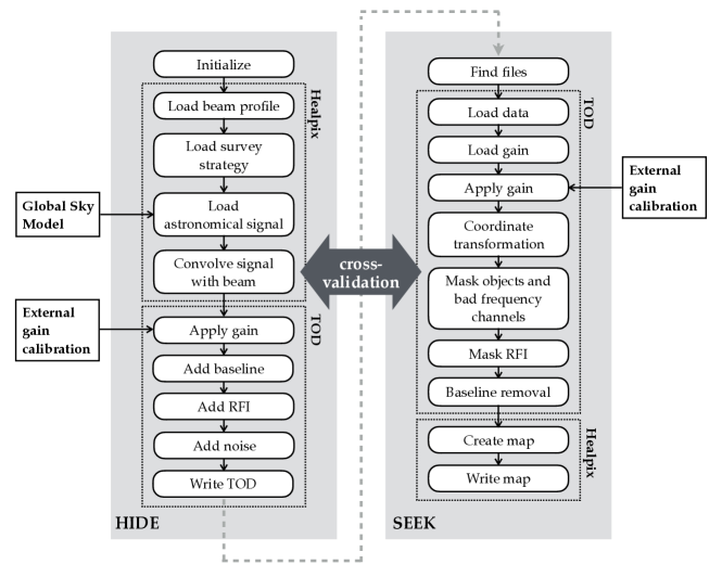
HIDE is a simulation pipeline for single-dish radio telescopes and SEEK is a data processing pipeline for observed or simulated radio telescope data. We have developed the two independent software packages simultaneously, which means that one pipeline can be used to cross validate the other. For example, in HIDE we simulate radio frequency interference (RFI) signals, while in SEEK we detect and mask the RFI signals. This suggests that the quality of the RFI masking in SEEK can be assessed using simulated data from HIDE. On the other hand, the goodness of the modeling in HIDE can be verified by processing real data with SEEK and comparing the results with the simulation. Both pipelines share a common design. Fig. 1 shows a schematic illustration of both packages.
To ensure the common design and facilitate the switching between HIDE & SEEK, both package are based on the simple plugin-based workflow engine Ivy, which we introduce in Section 2.1. In Section 2.2 we briefly describe the two main data structures that are used in HIDE & SEEK.
2.1 Ivy: Plugin-based workflow engine
Ivy is a generic workflow engine written in Python and is open-source under the GPLv3 license111http://github.com/cosmo-ethz/ivy. Its architecture ensures that individual elements of pipelines (which we refer as “plugins” here) are self-contained. The interaction between the plugins is done via a context object that is passed from plugin to plugin by the framework. Ivy’s design fosters reusability and maintainability of the code. As every plugin is loosely coupled to the pipeline and the other plugins, unit testing the individual components becomes greatly simplified. Furthermore, new features can easily be added to an existing pipeline in the form of a new plugin without interfering with the other plugins.
A pipeline developed with the Ivy framework always consists of a configuration file, that contains a list of the plugins that belong to this pipeline and parameters that are used by the plugins. An Ivy pipeline can be executed in parallel on multiple CPU cores with minimal work. By default Ivy uses Python’s built-in multiprocessing package but alternative parallelization scheme such as IPython cluster can be chosen. The workload is automatically distributed among the available CPU’s and Ivy executes the plugins in parallel.
2.2 Data structures: time-ordered data and Healpix maps
The two relevant data structures used in HIDE & SEEK are time-ordered data (TOD) and Healpix [14] maps. TOD refers to the data type we record at the end of the instrument chain (a bolometer or a spectrometer). Typically, one or multiple values that scale linearly with the signal received by the telescope is recorded over time. In our case, since the measurement instrument is a spectrometer, we have one value per frequency channel per time, which results in a 2D plane with time and frequency on the two axes (see Fig. 3 for an example of the observed and simulated TOD). This data format itself is agnostic about where the signal is from in the sky. Only by combining the data with the telescope pointing we map the TOD to the sky coordinates.
A Hierarchical Equal Area isoLatitude Pixelation (Healpix) map refers to a specific pixelation scheme implemented on a sphere. This format is commonly used in cosmology. Healpix maps have by construction equal-area pixels and the pixelation introduces minimal distortions and errors compared to other projection methods. Healpix maps can be manipulated with the Python wrapper Healpy222https://healpy.readthedocs.io. In this work, we use Healpix maps whenever the celestial coordinate is relevant. This includes the input Milky Way signal in HIDE and the final reconstructed map in SEEK.
2.3 HIDE architecture
HIDE & SEEK both follow the plugin design concept of the Ivy framework described above. The architecture allows the user to easily add new features or replace existing functionality. In the following, we give a high-level overview of the functionalities in both packages.
HIDE is a package for simulating a single dish radio telescope survey. As such, it takes Healpix maps as inputs and processes them into TOD. The design is flexible and can be customized to different instruments and survey designs. In the following, we describe the setup of the HIDE pipeline. This is not an exhaustive list for generic surveys and can easily be extended. The left half of Fig. 1 shows the structure of the pipeline and includes the following steps:
- Initialize
-
The Ivy configuration is loaded into memory and the random seed is initialized to ensure reproducible results.
- Load beam profile
-
A beam response pattern is loaded according to the configuration. The current design supports parametrized Gaussian or Airy [15] profiles and arbitrary beam patterns specified on a grid. The beam profiles can be frequency-dependent.
- Load survey strategy
-
The pointing of the telescope at a given time in the survey is computed according to the desired survey strategy. The plugin converts the telescope pointing from terrestrial coordinates (azimuth, elevation) into equatorial coordinates (RA, Dec). Different strategies can be chosen such as drift-scan surveys333A drift-scan is the survey mode where the telescope is fixed in the period of one day and changes the pointing of the telescope (mainly its elevation) from day to day. Due to the earth’s rotation, the telescope footprint on the sky “drifts” through the full 2 of RA positions at a given Dec on the celestial sphere., or a file-based scanning schedule such that a planned survey can be exactly simulated.
- Load astronomical signal
-
The astronomical signal used for the simulation is loaded. Here we use the Global Sky Model [GSM, 16], which is a synthetic model of the Milky Way as a function of frequency based on a large number of radio data sets. The GSM is stored as Healpix maps on a grid of frequencies and interpolated to the desired frequency when needed. The GSM maps are in units of brightness temperature (Kelvin).
- Convolve signals with beam
-
For each telescope pointing defined by the survey strategy, the telescope beam response is convolved with the astronomical signals and appended to the TOD array.
- Apply gain
-
To transform the TOD from units of Kelvin into internal units (Analog-to-digital unit, ADU) as recorded in the instrument, we multiply the TOD by a gain template. This information can come from external calibration or specifications of the instrument.
- Add baseline
-
An frequency and point dependent baseline offset is added to the TOD to account for contributions to the overall intensity from the instrument, the environment, etc. (see Section 3.1 for more details)
- Add RFI
-
A simulated RFI signal is added to the TOD array (see Section 3.1 for the specific model derived from data).
- Add noise
-
Gaussian (white) noise and and (pink) noise is added to the data to model noise contribution from the atmosphere and electronics.
- Write TOD
-
The simulations are written to disk in TOD format.
We note that the most computationally demanding step in the HIDE pipeline is the step of convolving the signals with the beam. We speed up this step by using Quaternions and a KD-tree data structure. The technical details of this operation is described in A.
2.4 SEEK architecture
SEEK is a flexible and easy-to-extend data processing pipeline for single dish radio telescopes. It takes the observed (or simulated) TOD in the time-frequency domain as an input and processes it into Healpix maps while applying calibration and automatically masking RFI. The data processing is parallelized using Ivy’s parallelization scheme.
We outline the setup of the SEEK pipeline below. Again, this list is not exhaustive but can easily be extended and modified given a different experiment. The structure of the SEEK pipeline is illustrated in the right half of Fig. 1 and includes the following steps:
- Find files
-
The file system is traversed to find simulated or observed data for a given time period and file-name convention.
- Load data
-
The data is loaded from the file system into memory and smoothed if specified by the user. SEEK is currently able to process both FITS [17] and HDF5444https://www.hdfgroup.org/HDF5 data formats. The design concept of Ivy ensures that the other plugins do not depend on the origin of the data. Therefore extending the support for further file formats can be implemented without interfering with the other functionalities.
- Apply gain
-
A gain factor is computed by using special calibration data that was collected on dedicated calibration days in the survey. Alternatively, an externally provided template can be loaded from the file system. This gain factor is applied to the TOD to convert the instrument-recorded values (ADU) to physical units (Kelvins).
- Coordinate transformation
-
The telescope pointing at each given time is connected to the TOD to give each pixel in the TOD a terrestrial coordinate. These coordinates are now transformed into equatorial coordinates corresponding to a given point in the celestial sphere.
- Mask objects and bad frequency channels
-
The TOD is masked if known bright objects such as the Sun and the Moon are too close to the telescope pointing. Furthermore, frequency bands known to be unusable (e.g., seriously contaminated by satellite communication bands) are masked.
- Mask RFI
-
The TOD is analyzed and pixels identified as contaminated by RFI are masked (see B for more details on SEEK’s automated RFI masking mechanism).
- Baseline removal
-
The baseline level per frequency is estimated from the median value over time of the cleaned TOD. This baseline is subtracted from the TOD.
- Create map
-
For every frequency channel the TOD is processed into a Healpix map. By default, each pixel in the Healpix map is filled with the mean value of all measurements in that pixel. One can also invoke an outlier-rejection step to avoid uncleaned RFI contaminating the mean.
- Write map
-
The Healpix maps and auxiliary information such as the frequency range and redshift information is written to disk in HDF5 file format.
In the SEEK pipeline, tackling the RFI is the most computationally challenging task. This includes both the RFI masking in the TOD plane and the final outlier-rejection applied at the Healpix map level. We describe our specific treatment of RFI in B.
2.5 Quality assurance
We developed HIDE & SEEK using best practice from software engineering. In particular, we use tools common in the Python community. Both packages follow a standardized packaging, which simplifies the development and installation including resolving dependent third party packages. The standardization released by the Python Package authority defines the directory structures of a package, which enforces the separation of functionality and makes it easier for new developers to engage in the project. Furthermore, it defines how to store meta-information of the package. In order to maintain a high level of quality and that newly developed features do not infer with existing code, we rigorously test the functionality of the packages with unit tests. To develop those tests we use the common testing framework py.test. Finally, both packages are fully documented using the standardized reStructuredText syntax such that we can automatically generate and publish a documentation555https://hide.readthedocs.io666https://seek.readthedocs.io using the Sphinx package.
3 Forward-modeling a Galactic survey at 990 – 1260 MHz with HIDE & SEEK
In this section, we describe how we apply HIDE & SEEK to model and analyze data for a mock Galactic survey. The design of this mock survey is based on the early Science Verification (SV) data from the Bleien Observatory as described in C16 and allows us to develop realistic models and test the robustness of the code. This data set was collected using a 7m single-dish telescope operating in drift-scan mode with a frequency range of 990 – 1260 MHz. In addition to the continuous scanning, calibration data was taken every 8 days to provide an anchor for various calibration tests. For more details of this data set, we refer the readers to C16.
We discuss below the survey-specific implementations that we have adopted in HIDE (Section 3.1) and SEEK (Section 3.2), respectively. For other experiments, these implementations may need to be modified or replaced. We then show an example of a forecast for the Galactic survey in Section 3.3 with the current pipelines.
3.1 Simulating a Galactic survey with HIDE
We customize the functionalities of HIDE to match the characteristics of the SV data from the Bleien Observatory. For the beam profile, or the angular response of our telescope, we use an Airy disk profile, which is a good approximation for an underilluminated 7m parabolic dish (C16). For the size of the beam, we use values inferred from transits of the Sun as described in C16. We generate data with MHz bandwidth between 990 MHz and 1260 MHz, resulting in 276 frequency channels. We use a drift-scan strategy that follows the schedule used in the SV data.
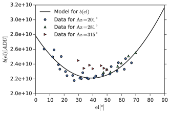
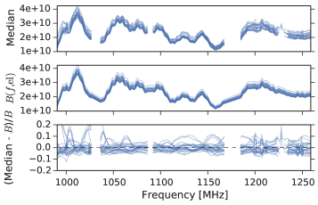
We make the simplified assumption that the TOD has a frequency- and elevation-dependent baseline that is otherwise independent of azimuth and time of the pointing as well as its Galactic coordinates. We furthermore assume that the frequency- and elevation-dependencies factorize, i.e. our baseline is given by
| (1) |
where is the frequency, is the elevation, is the frequency-dependent baseline and is a further elevation-dependent modulation of the baseline. To generate the model parameters for Eq. (1) that are motivated by data, we calculate the median of the TOD over a time window during the night (from midnight to 4:00 UT) over all survey days during SV after RFI mitigation. We then fit a second-order polynomial to the mean of the medians as a function of elevation (see Figure 2, left panel). Finally, we use the mean of the normalized medians as a model for the frequency-dependent baseline . In the right panel of Figure 2, we show the agreement between the observed medians and the calibrated model . We note that this is a simplified model. In D we discuss the influcence of day time and telescope pointing on the baseline for the SV data from the Bleien Observatory.
As shown in C16, the instrument noise in our TOD is very close to white noise due to the stable phase-switch implemented in the system. To model the amplitude of the noise, we estimate the standard deviation from TOD recorded in the night during SV. To avoid biases from RFI that was not properly mitigated, we estimate the scale of the noise per frequency channel as the mean of the and percentiles of the TOD for a given night. We use the mean of the estimated scales over all days for clean channels and the minimum over all days for the contaminated channels as model for the standard deviation of the TOD in units of ADU.
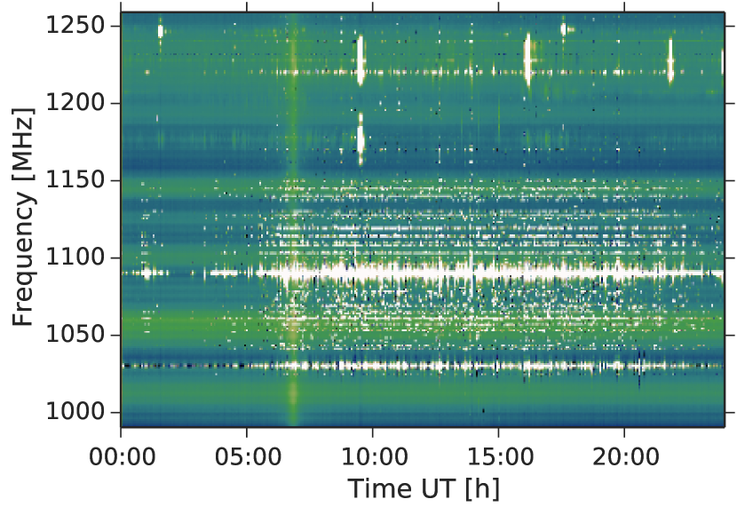
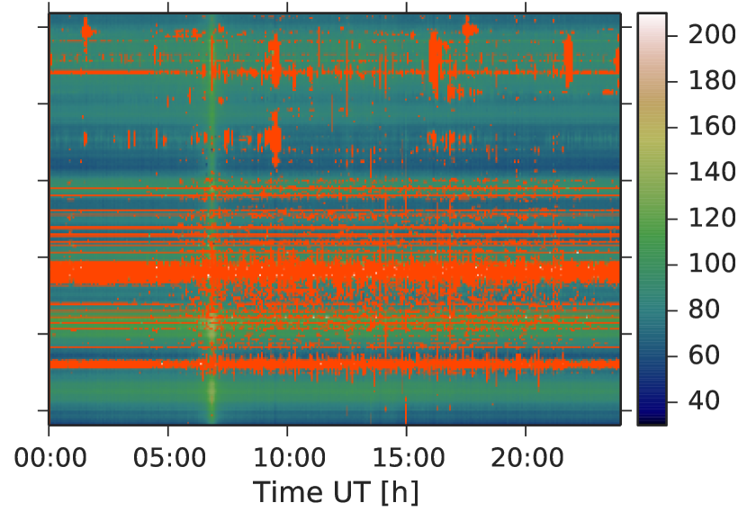
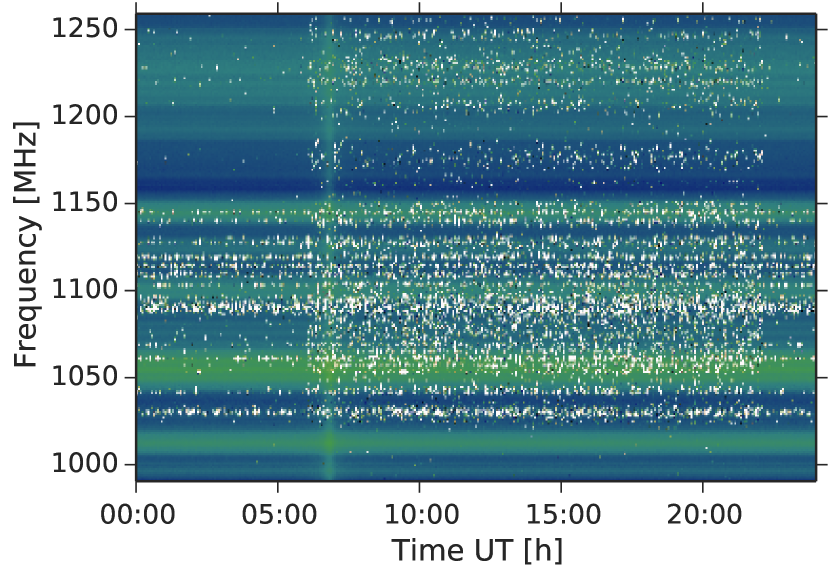
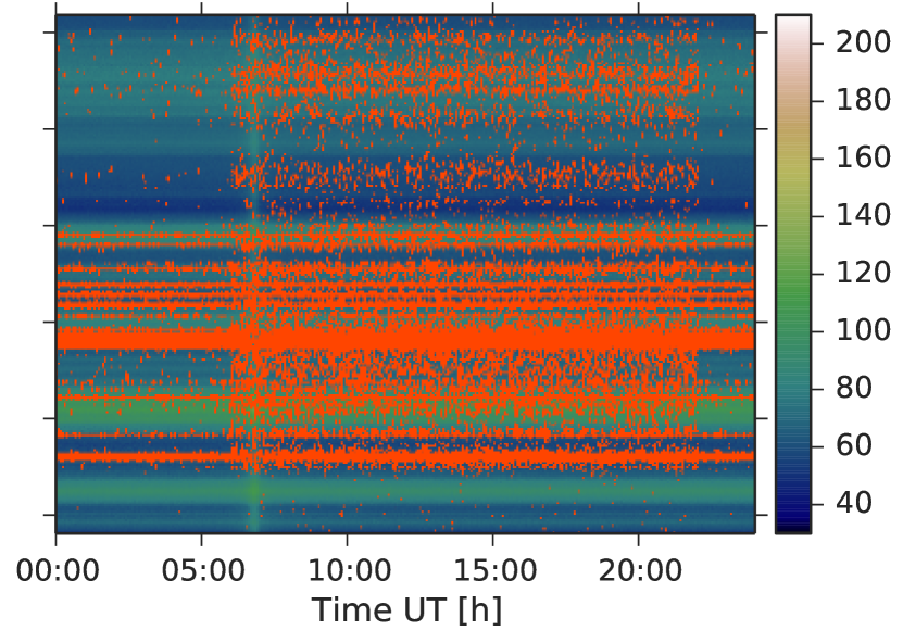
The Bleien Observatory is in a location with non-negligible RFI from human produced sources such as satellites and aircraft communication in the frequency range of interest. Due to the large variety of distinct RFI patterns, developing a realistic RFI model is challenging. As a result, we choose to adopt a simple model for the RFI, where each RFI burst is defined by the same profile in time and frequency (either exponential or Gaussian) and an amplitude. For each frequency, the amplitudes are sampled randomly from a uniform distribution between the standard deviation of the noise and a maximum value inferred from the real data. The rate of RFI bursts per frequency is chosen such that, on average, the number of pixels affected by RFI greater than the noise-level is matching the fraction of masked pixels inferred from the real data. This model can be implemented efficiently by starting with a zero time-frequency plane and setting the randomly chosen positions in time to the randomly drawn amplitudes for each frequency. The final simulated RFI is then given by a two-dimensional FFT convolution of the time-frequency plane with the chosen RFI profile. Figure 3 shows the TOD from the Bleien Observatory (first row) on March 21st, 2016, next to a simulated TOD from HIDE (second row). We note that even though this model is not capturing all aspects of the RFI, it approximately reproduces the RFI-induced data-loss and gives us the possibility to explore the performance of the RFI mitigation in SEEK.
3.2 Analyzing simulated data with SEEK
Next, we analyze the TOD and reconstruct the astronomical signals with SEEK. Having a simulation that is expected to be close to the observation allows us to implement a SEEK pipeline that can be used for the processing of the observation as well as simulation data with minimal modifications.
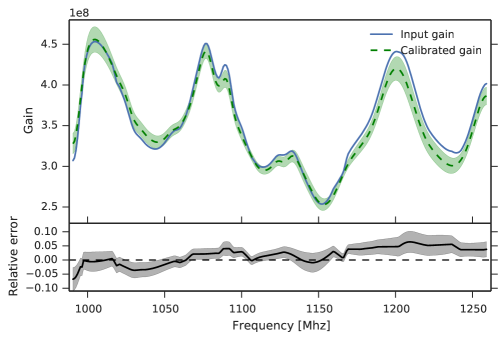
The first step after loading the TOD in the SEEK pipeline is to obtain the gain factor that converts the observed ADU values in the TOD into physical units. This procedure is referred to as flux calibration and the exact implementation is described in C. Fig. 4 shows the gain factors used for the simulation in HIDE (blue line) and the gain factor recovered from SEEK’s flux calibration. The accuracy of the flux calibration is biased by the RFI contamination and the noise in the data set. We use a simplified model and assume that is constant over time. From repeated measurements in SV we see variation in can vary up to .
For object-masking, we configure SEEK such that data is masked if the angular separation of the telescope pointing and the Sun is smaller than . Depending on the Moon phase data is masked if the separation is smaller than .
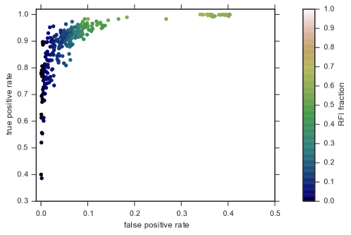
For RFI mitigation we have implemented the SumThreshold algorithm [18] with a morphological dilation of the resulting mask (for more details we refer to B). We set the parameters for the SumThreshold and mask dilation such that most of the RFI is being masked while minimizing the fraction of incorrectly masked data. The tuning of these parameters is done by analyzing the RFI masks of simulated data where the positions of the RFI pixels are exactly known. We then inspect the mask visually and statistically. Fig. 5 shows the receiver operating characteristic (ROC) curve of the mask obtained from SumThreshold and mask dilation. The x-axis displays the ratio of pixels incorrectly labeled as RFI and the y-axis represents the ratio of correctly masked pixels. Each point represents a different frequency while the color is showing the fraction of RFI in this channel. If the RFI contamination is low in a specific channel, SumThreshold has a low probability to mask the RFI pixels. As the fraction of contaminated pixels increases, the algorithm correctly masks the unwanted signal while maintaining a low rate of incorrectly masked clean pixels. In highly RFI-contaminated channels the true positive rate reaches almost . However, due to the high density of masked pixels, the mask dilation also increases the false positive rate.
Fig. 3 displays the visual inspection of a representative observed and simulated data set recorded on 21st of March 2016. The two left panels (observed and simulated TOD respectively) show the unmasked data where strong broad- and narrow-band RFI contamination is visible. The right panels show the same data overlaid with the RFI mask obtained from SumThreshold and mask dilation. Most of the RFI is well captured including weaker narrow-band RFI not visible in the left panels.
| Name | Value | |
| HIDE | Scanning strategy | Drift scan |
| Start date | 16.12.2015 | |
| End date | 26.05.2016 | |
| Telescope latitude | 47.344∘ | |
| Telescope longitude | 8.114∘ | |
| Dish diameter | 7 m | |
| Beam profile | Frequency-dependent Airy disk | |
| Astronomical signal | Global Sky Model with artificial calibration sources | |
| Near earth signal | Bleien horizon model (Fig. 2) | |
| RFI model | Bleien RFI model (Fig. 3) | |
| SEEK | Sum threshold | , smoothing kernel:4020 pixels |
| , | ||
| Mask dilation | Binary dilation with pixel structure | |
| Healpix map making | Pixel averaging with outlier rejection | |
| Minimum Sun separation | ||
| Minimum Moon separation | ||
| Healpix resolution | Nside=64 (0.84 deg2) |
3.3 Forecast
In this section we apply the full HIDE & SEEK framework to produce an end-to-end simulation for the mock Galactic survey described above. That is, given the survey design and our understanding of the data characteristics from the Bleien Observatory, we forecast the expected map of the Milky Way we will measure at the end of SV data collection after processing all the data through SEEK. We also forecast the expected signal-to-noise ratio of the observed Milky Way at different positions on the sky.
For this purpose, we set up a suite of HIDE simulations with the parameters listed in the top half of Table 1, and analyze the simulations using SEEK with the parameters listed in the bottom half of Table 1. These parameters are chosen to best match the SV data set from the Bleien Observatory. We show examples of the resulting Healpix maps for this forecast run at 991.5 MHz in the top-left panel of Fig. 6. To obtain the pure “signal” for the signal-to-noise calculation described below, we also create a second HIDE simulation without observational effects such as noise, RFI, gain, and baseline. Analyzing this second simulation with SEEK yields a map that is convolved in the same way as the forecasted map, but does not suffer from any other observational effects.
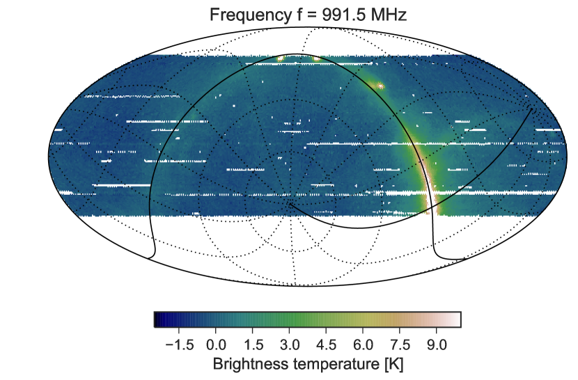
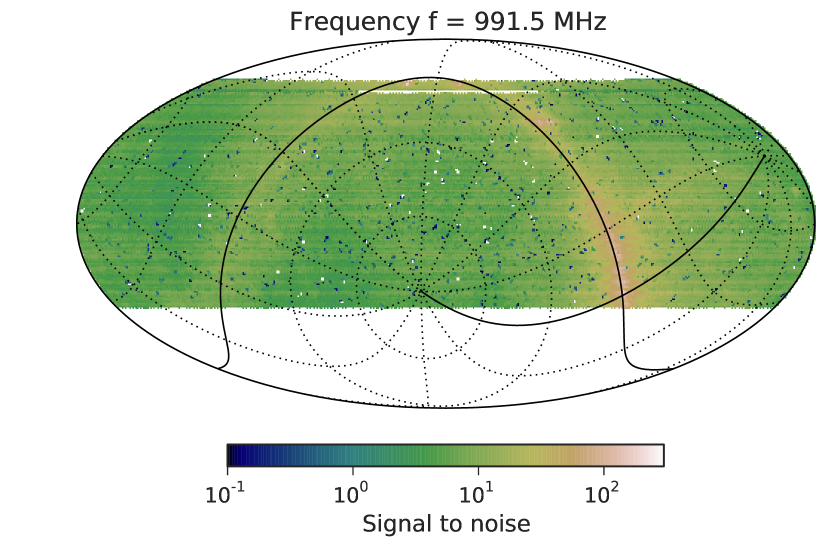
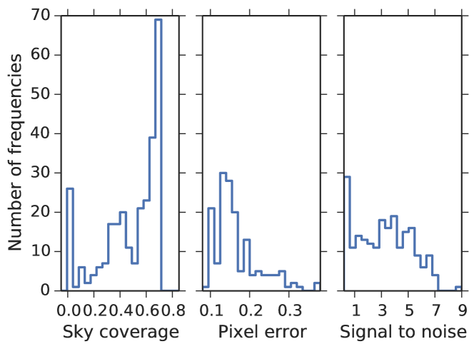
From the SV data, we inferred strong variations of the RFI contamination over frequencies as well as time of day. RFI from airplane communication, for example, only happens during the day as Zurich airport is open from 6:00 am to 11:00 pm UT and affects the TOD in the frequency range from MHz to MHz (see Fig. 3, top left panel). As RFI leads to data-loss, both the signal to noise and the sky coverage of our forecasts depend on frequency. We define signal-to-noise of a pixel in a given frequency channel as the ratio between the clean simulation (signal) and the uncertainty in the forecasted map estimated from the standard deviation in each pixel (noise). As an example, we show the signal-to-noise map at a frequency of 991.5 MHz in the top-right panel of Fig. 6. We further define the sky coverage as the ratio between the number of pixels with at least 2 observations (which can come either from different passes of the drift scan or different time dumps of the same pass) and the total number of pixels in the sky.
In the lower right panel of Fig. 6 we show the distribution over frequencies of the total sky coverage, median noise, and median signal-to-noise for our forecasts simulations. We find an overall median signal-to-noise of 2.3. The median signal-to-noise is 6.5 at the Galactic plane, 2.8 – 3.4 at 20 degrees, 2.0 – 2.6 at 40 degees and 1.6 – 2.5 at 60 degrees off the plane. The best frequencies in the ranges 990 MHz to 1010 MHz and 1185 MHz to 1195 MHz achieve a median signal-to-noise of approximately 9 and 8, respectively. For the noise in our maps, we find a median error of 0.24 K and a median effective integration time of 149 sec. The best frequency range from 1185 MHz to 1195 MHz reaches an error of 0.09 K. Finally, the median sky coverage is given by 57% and the highest values of 70% are achieved by the channels from 990 MHz to 1010 MHz.
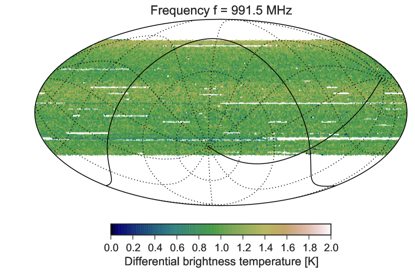
We also study systematic differences between the forecasted and the map without observational effects by looking at the difference map between them shown in the lower left panel of Fig. 6. We find that the systematic differences in the maps are due to cumulated inaccuracies of the reconstruction of baseline and gain described in section 3.2 as well as unmitigated RFI. The mild elevation dependent stripes in Fig. 6 imply that the dominant contribution to the systematics is coming from the baseline correction which is the only elevation-dependent artifact in the simulations. We defer the development of a more complicated and realistic baseline removal to future work. This uncertainty associated with the baseline removal increases the total noise and lowers the signal-to-noise ratio of the maps. The overall median signal-to-noise with systematic uncertainty is 2.0, with a median signal-to-noise of 6.3 at the Galactic plane, 2.8 – 3.5 at 20 degrees, 2.0 – 2.7 at 40 degees and 1.7 – 2.6 at 60 degrees off the plane. A median signal-to-noise of 5 – 6 is achieved in the cleanest frequency channels.
4 Conclusion
In this paper, we present two software packages, HIDE & SEEK, for simulating and processing data from single-dish radio surveys. HIDE simulates the entire system chain of a radio telescope from the astronomical signal to the time-ordered-data (TOD). SEEK on the other hand processes simulated and real observed TOD to Healpix maps while calibrating the signal and automatically masking contamination from radio frequency interference (RFI). The two packages together provide an end-to-end forward-modeling framework that can be used to systematically understand and test the various steps in the data processing procedure. They can also be used independently if only simulation or data processing is needed. The packages were developed based on the data taken at the Bleien Observatory, but can be easily adjusted to model and process similar projects. The other strength of using both HIDE & SEEK is the possibility to perform cross-validation between the simulation and the analysis algorithm. We demonstrate how the two packages are used together to study systematic effects such as imperfect baseline removal and RFI leakage.
We present the main architecture of the codes and how typical data is simulated and processed. We then describe more specifically how we apply the two packages to a forward-modeling exercise of a Galactic survey at 990 – 1260 MHz. We use HIDE to simulate the entire survey with the main survey characteristics matched to the Science Verification data from the Bleien Observatory. We then process this simulated data with SEEK, using settings close to that used for the observed data. The result of this forward model is a forecast of the expected output from an idealized Galactic survey, with simplifications that are well-understood. We predict a median sky coverage of 50% and a median signal-to-noise ratio of 2.3. In the channels from 990 MHz to 1010 MHz we expect a total sky coverage up to 70% with median signal-to-noise ratio of approximately 9 without systematic errors and 5 – 6 with systematic errors.
HIDE & SEEK follow common software engineering best practices. Being compliant with well-established coding standards, they offer great flexibility for defining data processing pipelines. Although some of the current implementations in HIDE & SEEK are relatively simple and more general compared to existing software such as [19, 20, 11], they have the advantage of being open-source code with a rigorous structure, and thus provide an easy-to-use foundation to build upon for more complicated functionalities. We have developed both packages in pure Python and increase the performance of computationally intensive parts by just-in-time compilation. By doing so, we are able to perform the RFI mitigation of the TOD in SEEK at an rate of 190-200 GB/h/CPU. Using Ivy’s parallelization scheme, we can furthermore distribute the workload to multiple cores and make efficient use of the available hardware. This allows us to easily process the expected data volume from a five-month survey on a modern laptop. In HIDE we implemented an efficient beam convolution on the sphere by using Quaternions combined with a KD-Tree. Creating the simulations for the Galactic survey with HIDE took around 3 hours on a single-core of an average notebook. Further information such as documentation of the software can be found at http://hideseek.phys.ethz.ch/.
Appendix A Implementation of beam convolution on a sphere
In order to convolve the beam response with the simulated astronomical signal, we have to rotate the grid that defines the beam geometry on a sphere. As this step is repeated for every telescope pointing defined by the scanning strategy as well as for every simulated frequency, high efficiency for the operation is crucial.
Conventionally, spherical rotations are implemented by using the Euler matrix rotation. Applying this rotation scheme to a Healpix map requires transforming the spherical pointing angles ( and ) into Euler coordinates (). This involves computing the rotation matrix , applying this matrix to the coordinate vector, transforming the results back into spherical coordinates, and finally performing the convolution. Typically, applying rotation on multiple axes requires a repetition of the above steps for each axis. This can be computationally even more demanding and numerically less stable.
We have implemented all the coordinate rotations with Quaternions, a technique commonly used in 3D computer vision [21]. Rotations over multiple axes can be concentrated into one operation with Quaternions, which make them computationally more efficient and stable. Furthermore they do not suffer from the so-called gimbal lock as Euler rotation do, where a rotation along one axis may produce coordinates that do not allow further rotations [21].
Additionally, this allowed us to easily implement a lookup table with a binary search for the and function to further speed up the rotations. In order to efficiently find the pixels relevant for the rotation of the beam geometry we also use store all the Healpix pixel information in a KD-Tree adapted for spherical coordinates.
Appendix B RFI masking
The SEEK package was designed to be able to process data that is heavily contaminated with RFI. SEEK’s automated RFI masking mechanism is based on two steps: the SumThreshold algorithm and a Healpix pixel-based outlier rejection. The SumThreshold method was first proposed in [18] and since then successfully implemented in different radio processing pipelines [e.g., 19, 20]. Its simple concept and high detection efficiency makes it an attractive candidate for the SEEK package.
SumThreshold gradually builds a mask that flags the unwanted RFI in the data. The underlying assumption of the algorithm is that the astronomical signal is relatively smooth in both time and frequency (i.e., on the TOD plane), while RFI signals have sharp edges. Under this assumption, SumThreshold iteratively improves a model of the true astronomical signal by smoothing the TOD with a Gaussian filter. It then clips pixels that lie above a certain threshold after subtracting this model from the data. The masking naturally starts with localized, strong RFI bursts. The threshold is progressively lowered in each iteration such that more RFI is detected and masked along the process. We also take into account that RFI often extends in both time and frequency directions. That is, the algorithm combines neighboring pixels and masks them if their sum exceeds a threshold. Due to this underlying assumption SumThreshold has to be applied with precaution to spectral line data, which can show non-smooth signatures. RFI originating from radio point sources, such as planes or satellites is well captured. However, depending on the instrument configuration natural point sources could be incorrectly masked by the algorithm.
Finally, we apply a morphological dilation of the mask, i.e. we enlarge the mask depending on the density of masked pixels in a region in order to capture possible missed RFI leakage. The iterative Gaussian smoothing in the presence of a mask is the most computationally intensive part. In order to accelerate the process while keeping the code fully Python, we use the HOPE just-in-time compiler package [22], which translates the Python code into C++ and compiles at runtime. This allows SEEK to perform the RFI mitigation step at a rate of 190-200 GB/h/CPU, which is faster than other existing Python implementations of the similar algorithm [e.g. 20].
The second step in the RFI mitigation is applied during the Healpix map-making process. Pixel values belonging to the same Healpix pixel and same frequency are analyzed in order to remove outliers. We use a simple but robust outlier criterion defined through , where
with
where is the median of , the median of and a predefined threshold. This replaces the mean and standard deviation often used in sigma clipping, which can be biased toward the outliers.
Appendix C Flux calibration
We are interested in converting the raw data value that is recorded in the native instrument units of ADU into a brightness temperature with the units of Kelvin – this process is referred as flux calibration. Brightness temperature is a measure of the luminosity of the source under a given resolution, and is independent of other instrument properties. We refer to this conversion as “Gain” , or
| (2) |
For the data set used in this work, calibration data taken during the survey consists of several transit measurements of astronomical sources with well known spectra. Transit measurements are taken with the telescope parked at some position on the sky where the source of interest is expected to cross due to the rotation of the Earth. The data from these transits give an estimate of the beam response profile. Since we know the spectra of these sources, we can derive given our knowledge of the beam.
| (3) |
where is the wavelength in meters, is the effective aperture size of the instrument in square meters, is the Planck constant, is the spectral density of the reference source in Jansky (10), and is the measured ADU value at the peak of the transit for the reference source. is defined through
| (4) |
where is the beam solid angle defined
| (5) |
and is the beam profile with its peak normalized to 1.
We calculate assuming the an Airy disk profile with size measured from transit data of the Sun. For , since we are only interested in the main beam here, we fit the transit data with a Gaussian profile.
Appendix D Apply SEEK to SV data at the Bleien Observatory
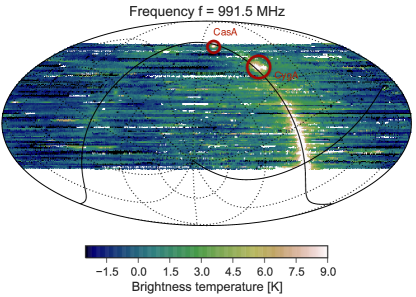
We have used SEEK to process the SV data from Bleien (see C16 for details of the SV data) to demonstrate the usability of SEEK on real data. Fig. 7 shows the resulting map at MHz with MHz bandwidth at a Healpix resolution of nside. The Galactic plane is clearly visible, as well as the brightest point sources close to the plane such as Cassiopeia A and Cygnus A. There are, however, clear patterns of stripes in the declination direction in the map, which corresponds to the drift-scan pattern used in the SV data. These patterns originate from a time-varying baseline which varies on the time scale of several hours and cannot be removed with our simple baseline-removal method in SEEK. The baseline also appears to be correlated with the ambient temperature and thus higher during day time. This coincides with the time where the Galactic center is observed in the SV months, making the Galactic center brighter than expected. Furthermore, comparing Fig. 7 and Fig. 6, we see a higher masked area in the data, which originates from artifacts in the data that were manually masked. These artifacts appear as broad-band, bright bursts that are potentially related to the moisture on the cover of the feed horn.
After a quantitative analysis of the maps from SV, we find that the statistical uncertainty of the maps are close to expectation from the simulations. However, the systematic uncertainties associated with the varying baseline will limit the usage of these maps in cosmological studies. We conclude that the stability of the overall system needs to be improved. Although the electronic chain described in C16 is stable, the existing observatory environment and other supporting infrastructure still need further upgrades to meet the stringent requirements set for cosmological surveys.
Below, we discuss several aspects of the system stability that we plan on improving in the future. In parallel, we will also work on incorporating these effects in the HIDE simulations and developing more sophisticated baseline-removal techniques in SEEK. First, the temperature of the main electronics is only controlled by a moderate heating system which can regulate temperature swings up to 40 degrees. Unfortunately, during the survey, there were several occasions where the temperature change exceeded this range and the electronic temperature was no longer regulated, which in turn resulted in fluctuations of the baseline. Furthermore, temperature at the feed horn is not controlled, which adds to the baseline instability. Second, the frontend electronics were not properly shielded. This means that water from rain and dew leaks in under extreme weather conditions, and the frontend is more heated by the Sun at certain pointing directions than others. During the SV observations, there were incidents of heavy rainfall that caused the frontend to response strangely and/or stop responding.
All these valuable lessons learned from studying the SV data will feed into the next stage of observations at the Bleien Observatory as well as other future surveys.
Appendix E Code distribution
Detailed documentation and installation instructions can be found on the package website http://hideseek.phys.ethz.ch/. The HIDE & SEEK packages are released under the GPLv3 license The development is coordinated on GitHub http://github.com/cosmo-ethz/hide and http://github.com/cosmo-ethz/seek. We welcome all contributions to the code development.
Appendix F TOD file format
The default TOD file format and structure used in HIDE & SEEK are designed to be consistent with that collected at the Bleien Observatory. All files are in HDF5 file formats, and are compressed using the common lossless gzip compression. Each HDF5 file contains several “dataset” units. Four datasets are used to store the time-frequency planes (“P/Phase0”, “P/Phase1”, ‘P2/Phase0”, and “P2/Phase1”) and an additional dataset for the time-axis that records the time-stamp for each pixel (“TIME”). The structure of the four time-frequency planes originated from the special design of the BGS project777These four time-frequency planes include both the measured spectrum () and the measured squared spectrum () for both voltage phases ( and )., but one can easily adapt HIDE & SEEK to a different file format.
References
- [1] M. Reinecke, K. Dolag, R. Hell, M. Bartelmann, T. Enßlin, A simulation pipeline for the planck mission, Astronomy & Astrophysics 445 (1) (2006) 373–373.
- [2] B. Nord, A. Amara, A. Réfrégier, L. Gamper, L. Gamper, B. Hambrecht, C. Chang, J. Forero-Romero, S. Serrano, C. Cunha, et al., Spokes: An end-to-end simulation facility for spectroscopic cosmological surveys, Astronomy and Computing 15 (2016) 1–15.
- [3] S. Bridle, J. Shawe-Taylor, A. Amara, D. Applegate, S. T. Balan, J. Berge, G. Bernstein, H. Dahle, T. Erben, M. Gill, et al., Handbook for the great08 challenge: An image analysis competition for cosmological lensing, The Annals of Applied Statistics (2009) 6–37.
- [4] A. Refregier, A. Amara, A way forward for cosmic shear: Monte-carlo control loops, Physics of the Dark Universe 3 (2014) 1–3.
- [5] C. Bruderer, C. Chang, A. Refregier, A. Amara, J. Berge, L. Gamper, Calibrated ultra fast image simulations for the dark energy survey, arXiv preprint arXiv:1504.02778.
- [6] J. R. Peterson, J. G. Jernigan, S. M. Kahn, A. P. Rasmussen, E. Peng, Z. Ahmad, J. Bankert, C. Chang, C. Claver, D. K. Gilmore, E. Grace, M. Hannel, M. Hodge, S. Lorenz, A. Lupu, A. Meert, S. Nagarajan, N. Todd, A. Winans, M. Young, Simulation of Astronomical Images from Optical Survey Telescopes Using a Comprehensive Photon Monte Carlo Approach, ApJS218 (2015) 14. arXiv:1504.06570, doi:10.1088/0067-0049/218/1/14.
- [7] R. A. Battye, I. W. A. Browne, C. Dickinson, G. Heron, B. Maffei, A. Pourtsidou, H I intensity mapping: a single dish approach, MNRAS434 (2013) 1239–1256. arXiv:1209.0343, doi:10.1093/mnras/stt1082.
- [8] M. Santos, P. Bull, D. Alonso, S. Camera, P. Ferreira, G. Bernardi, R. Maartens, M. Viel, F. Villaescusa-Navarro, F. B. Abdalla, M. Jarvis, R. B. Metcalf, A. Pourtsidou, L. Wolz, Cosmology from a SKA HI intensity mapping survey, Advancing Astrophysics with the Square Kilometre Array (AASKA14) (2015) 19arXiv:1501.03989.
- [9] M.-A. Bigot-Sazy, Y.-Z. Ma, R. A. Battye, I. W. A. Browne, T. Chen, C. Dickinson, S. Harper, B. Maffei, L. C. Olivari, P. N. Wilkinsondagger, HI Intensity Mapping with FAST, in: L. Qain, D. Li (Eds.), Frontiers in Radio Astronomy and FAST Early Sciences Symposium 2015, Vol. 502 of Astronomical Society of the Pacific Conference Series, 2016, p. 41. arXiv:1511.03006.
- [10] J. D. Swinbank, T. D. Staley, G. J. Molenaar, E. Rol, A. Rowlinson, B. Scheers, H. Spreeuw, M. E. Bell, J. W. Broderick, D. Carbone, H. Garsden, A. J. van der Horst, C. J. Law, M. Wise, R. P. Breton, Y. Cendes, S. Corbel, J. Eislöffel, H. Falcke, R. Fender, J.-M. Grießmeier, J. W. T. Hessels, B. W. Stappers, A. J. Stewart, R. A. M. J. Wijers, R. Wijnands, P. Zarka, The LOFAR Transients Pipeline, Astronomy and Computing 11 (2015) 25–48. arXiv:1503.01526, doi:10.1016/j.ascom.2015.03.002.
- [11] J. P. McMullin, B. Waters, D. Schiebel, W. Young, K. Golap, CASA Architecture and Applications, in: R. A. Shaw, F. Hill, D. J. Bell (Eds.), Astronomical Data Analysis Software and Systems XVI, Vol. 376 of Astronomical Society of the Pacific Conference Series, 2007, p. 127.
- [12] R. Dodson, K. Vinsen, C. Wu, A. Popping, M. Meyer, A. Wicenec, P. Quinn, J. van Gorkom, E. Momjian, Imaging SKA-scale data in three different computing environments, Astronomy and Computing 14 (2016) 8–22. arXiv:1511.00401, doi:10.1016/j.ascom.2015.10.007.
- [13] C. Chang, C. Monstein, J. Akeret, S. Seehars, A. Refregier, A. Amara, A. Glauser, B. Stuber, An Integrated System at the Bleien Observatory for Mapping the Galaxy, ArXiv e-printsarXiv:1607.07451.
- [14] K. M. Górski, E. Hivon, A. J. Banday, B. D. Wandelt, F. K. Hansen, M. Reinecke, M. Bartelmann, HEALPix: A Framework for High-Resolution Discretization and Fast Analysis of Data Distributed on the Sphere, ApJ622 (2005) 759–771. arXiv:astro-ph/0409513, doi:10.1086/427976.
- [15] G. B. Airy, Ueber die Diffraction eines Objectivs mit kreisrunder Apertur, Annalen der Physik 121 (1838) 86–95. doi:10.1002/andp.18381210906.
- [16] A. de Oliveira-Costa, M. Tegmark, B. M. Gaensler, J. Jonas, T. L. Landecker, P. Reich, A model of diffuse Galactic radio emission from 10 MHz to 100 GHz, MNRAS388 (2008) 247–260. arXiv:0802.1525, doi:10.1111/j.1365-2966.2008.13376.x.
- [17] D. C. Wells, E. W. Greisen, R. H. Harten, FITS - a Flexible Image Transport System, A&AS44 (1981) 363.
- [18] A. Offringa, A. de Bruyn, M. Biehl, S. Zaroubi, G. Bernardi, V. Pandey, Post-correlation radio frequency interference classification methods, Monthly Notices of the Royal Astronomical Society 405 (1) (2010) 155–167.
- [19] A. Offringa, A. de Bruyn, S. Zaroubi, M. Biehl, A lofar rfi detection pipeline and its first results, arXiv preprint arXiv:1007.2089.
- [20] L. W. Peck, D. M. Fenech, Serpent: Automated reduction and rfi-mitigation software for e-merlin, Astronomy and Computing 2 (2013) 54–66.
- [21] K. Shoemake, Animating rotation with quaternion curves, in: ACM SIGGRAPH computer graphics, Vol. 19, ACM, 1985, pp. 245–254.
- [22] J. Akeret, L. Gamper, A. Amara, A. Refregier, Hope: A python just-in-time compiler for astrophysical computations, Astronomy and Computing 10 (2015) 1–8.