Quantifying Uncertainties in Fault Slip Distribution during the Tōhoku Tsunami using Polynomial Chaos

Abstract

An efficient method for inferring Manning’s $n$ coefficients using water surface elevation data was presented in Sraj et al. [1] focusing on a test case based on data collected during the Tōhoku earthquake and tsunami. Polynomial chaos expansions were used to build an inexpensive surrogate for the numerical model GeoClaw, which were then used to perform a sensitivity analysis in addition to the inversion. In this paper, a new analysis is performed with the goal of inferring the fault slip distribution of the Tōhoku earthquake using a similar problem setup. The same approach to constructing the PC surrogate did not lead to a converging expansion, however an alternative approach based on Basis-Pursuit DeNoising was found to be suitable. Our result shows that the fault slip distribution can be inferred using water surface elevation data whereas the inferred values minimizes the error between observations and the numerical model. The numerical approach and the resulting inversion are presented in this work.

1 Introduction

Natural disasters impacting coastlines have long been some of the most dangerous and unpredictable of all natural hazards, and among these tsunamis are particularly devastating. Due to their rarity, it is extremely challenging to accurately understand and predict these events, owing to the uncertainties in their generation, primarily subduction zone earthquakes, and evolution, primarily the characterization of physical processes and bathymetric measurements. Quantifying such uncertainties using available past event data is critical to help guide decision making during and after an event and also assists in building more accurate models.

One of the greatest sources of uncertainty in tsunami modeling lies with the earthquake that generates the tsunami. This is mitigated in the far field by the nature of the shallow water equations but in the near-field this uncertainty can lead to significant discrepancies between predicted and actual flooding. This is particularly troublesome when attempting to forecast tsunami run-up as the immediately available fault movement is coarse in resolution and highly uncertain itself. To mitigate this and improve the understanding of these predictions, we propose an avenue for reconstructing the slip motion based on tsunami observations immediately available via the DART buoy system.

A number of efforts towards quantification of uncertainty in the context of tsunamis have been undertaken. Some studies have looked at fitting multiple earthquake models, attempting to ascertain the best fit to available data while allowing for simple variation in their initiation [2], while others have looked at other types of generation mechanisms such as land-slide generated tsunamis [3]. Similar approaches to other problems within the context of the ocean have also been presented. Examples of these include studies examining tidal simulations that employed an adjoint or Kalman filtering based approach [4, 5, 6, 7, 8]. Recently, the authors also presented an efficient method for the inversion of Manning’s $n$ coefficients that used water surface elevation data collected during the Tōhoku earthquake and tsunami [1]. The efficiency of the method stems from using a Polynomial Chaos (PC) surrogate model that approximated the forward model GeoClaw simulating the tsunami. The surrogate was constructed using a non-intrusive spectral projection (NISP) method and was used within a Bayesian inference formalism to avoid multiple runs of the forward model. We note that Bayesian inversion of the distribution of fault slip has also been studied using synthetic data of surface displacement [9].

The PC method uses polynomials to approximate a forward model (or a function) and has been employed in the literature in various applications including large-scale models [10, 11, 12, 13, 14]. In those applications, traditional spectral projection methods [12, 15, 16] to construct the PC model were successfully implemented. In recent studies, however, the spectral projection technique failed to construct faithfully a PC expansion that represents the forward model [17, 55]. This was due to the non-linearity of the forward model and to the internal noise that was present, leading to PC expansion convergence issues. Instead, a compressed sensing technique called Basis-Pursuit-DeNoising (BPDN) was implemented to determine the PC expansion coefficients [19]. This technique first estimates the noise in the model (if any) and then solves an optimization problem to determine the PC expansion coefficients by assuming sparsity in the coefficients and fitting the PC surrogate to a set of random model runs subject to the estimated noise. BPDN was also recently implemented to build a proxy model for an ocean model with initial and wind forcing uncertainties [20]. In that application, there was no noise in the model outputs, however, the BPDN method was used as it does not require simulations at pre-specified sets of parameters which is a requirement by the NISP method.

In this work, we seek to quantify the uncertainties of the generating earthquake by parameterizing the slip field in space. The basic approach is the same as the one employed in [1] where a Polynomial Chaos (PC) surrogate is constructed [21, 22] and used for the inversion process using Bayesian inference [23]. In the case of the parameterized slip field, however, the specific method of constructing a PC surrogate using the NISP method was not successful. Instead the BDPN method proved more effective and capable of overcoming the convergence issues of the NISP approach and is the primary contribution presented in this paper. We also present results that show the ability of inferring the fault slip distribution using the DART buoys.

The remainder of the article is laid out as follows. In Section 2, the essential setup of the forward model is briefly described as well as the earthquake parameterization considered. In Section 3, the formulation of the inverse problem including the approaches explored for the construction of the polynomial chaos surrogate are detailed. Section 4 presents results of the PC construction using both NISP and BPDN methods in addition to results of the forward and inverse problems. Finally a discussion of the results and some conclusions are outlined in Section 5.

2 Problem Setup

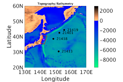
The Tōhoku tsunami of 2011 was the most observed tsunami in history providing us with a wealth of observational data. The earthquake had an estimated magnitude of 9.0 ($\text{M}_{\text{w}}$) causing massive damage across Japan due to the earthquake alone. The epicenter of the earthquake was located approximately 72 km east of the Tōhoku region as indicated in Figure 1(Left). This section is devoted to the description of the forward model used to simulate the tsunami and the parameterization of the earthquake slip field.

2.1 Forward Model

The forward numerical model employed in this study is GeoClaw, a package that has been used to model a number of geophysical phenomena, mostly notably tsunamis for which it has been validated and approved for hazard mapping projects [25]. It solves the non-linear, two-dimensional shallow water equations

$$\frac{\partial{}}{\partial{t}}h+\frac{\partial{}}{\partial{x}}(hu)+\frac{\partial{}}{\partial{y}}(hv)=0,$$ (1)

$$\frac{\partial{}}{\partial{t}}(hu)+\frac{\partial{}}{\partial{x}}\left(hu^{2}+\frac{1}{2}gh^{2}\right)+\frac{\partial{}}{\partial{y}}(huv)=~{}~{}fhv-gh\frac{\partial{}}{\partial{x}}b-C_{f}|{\mathchoice{\mbox{\boldmath$\displaystyle{u}$}}{\mbox{\boldmath$\textstyle{u}$}}{\mbox{\boldmath$\scriptstyle{u}$}}{\mbox{\boldmath$\scriptscriptstyle{u}$}}}|hu,$$

$$\frac{\partial{}}{\partial{t}}(hv)+\frac{\partial{}}{\partial{x}}(huv)+\frac{\partial{}}{\partial{y}}\left(hv^{2}+\frac{1}{2}gh^{2}\right)=-fhu-gh\frac{\partial{}}{\partial{y}}b-C_{f}|{\mathchoice{\mbox{\boldmath$\displaystyle{u}$}}{\mbox{\boldmath$\textstyle{u}$}}{\mbox{\boldmath$\scriptstyle{u}$}}{\mbox{\boldmath$\scriptscriptstyle{u}$}}}|hv,$$

where $h$ is the depth of the water column, $u$ and $v$ the velocities in the longitudinal and latitudinal directions respectively, $g$ the acceleration due to gravity, $b$ the bathymetry, $f$ the Coriolis parameter, and $C_{f}$ the bottom friction coefficient. The sea-surface anomaly $\eta$, the difference between a specified datum, such as mean tide level, and the modeled sea-surface, is $\eta=h+b$.

GeoClaw is an off-shoot of Clawpack that solves systems of hyperbolic equations in conservative and non-conservative form. The primary computational kernel is the Riemann solver which determines fluctuations, wave speeds and strengths. The Riemann solver in GeoClaw contains a number of features relevant to tsunami modeling including: (1) inundation (flooding at the shore); (2) well-balanced formulation, providing the ability to handle topographical features while maintaining steady-states (most notably an ocean at rest); and (3) inclusion of entropy correction that handle rarefaction of the flow [26]. One of the key components that makes GeoClaw effective at modeling trans-oceanic tsunamis is its use of adaptive mesh refinement (AMR). AMR allows resolution of the model to follow features of the solution of interest, such as the wave height difference from sea-level. GeoClaw implements these schemes via block-structured AMR as detailed in [27, 28].

Much of the setup for the Tōhoku simulations presented was adapted from the GeoClaw simulations presented in [2] including the refinement strategy. This includes resolutions ranging from 1 degree in both longitude and latitude to 75” resolution. The bathymetry used here is a combination of ETOPO 1’ and 4’ resolution data [29]; the finer bathymetry used in [2] to model inundation appropriately was excluded as this study does not include inundation data in the inversion.

2.2 Parametric Representation of the Slip Distribution

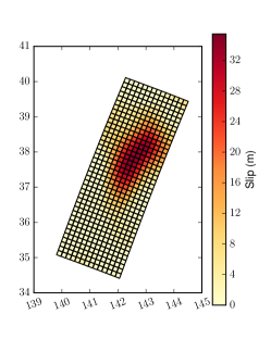
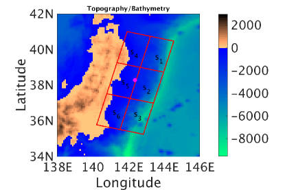
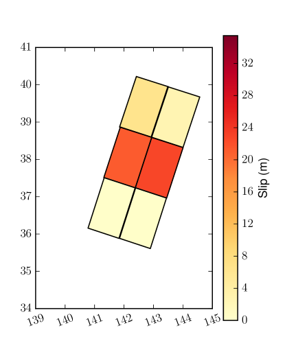
The overall goal of this article is to invert for the source earthquake using observational data available immediately after the earthquake. In order to simplify the investigation of the problem formulation, the base geometry of the fault was assumed fixed while the slip on the fault is assumed to be uncertain. Based on previous inversions, the slip magnitude was constrained between the similar slips proposed in [30] of $s_{max}=30~{}m$ and no-slip $s_{min}=0~{}m$ (see Figure 1 right). Additionally the fault was broken up into 6 sub-regions of which each can have a unique slip value in the inversion (see Figure 2) and cover the largest area of slip. The initial uncertainty was represented as a non-informative, uniform distribution with the limits mentioned above. The uncertainty is then quantified through PC expansions as in [12, 13].

3 Formulation

In this section, we describe the different steps of our method to numerically solve the inverse problem stated above. In Section 3.1, we analyze the available observations used in the Bayesian inference step, outlined in Section 3.2. Finally, in Section 3.3, we provide some details on a key ingredient of our methodology i.e. constructing a surrogate of the forward model for the sake of accelerating the Bayesian inference.

3.1 Observations

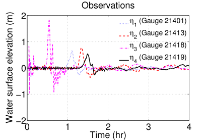
We use observations consisting of water surface elevation measurements collected for a period of around $4$ hours during the event at four different gauge locations. These gauges are part of the Deep-ocean Assessment and Reporting of Tsunamis (DART) buoy system developed and maintained by the National Oceanic and Atmospheric Administration (NOAA) with the purpose of providing early-warning detection and forecasting of tsunami propagation in the Pacific Ocean [31]. The four selected gauges are the closest to the earthquake source of the Tōhoku tsunami denoted by Gauge 21401, 21413, 21418, and 21419. The locations of these buoys are shown in Figure 1 (Left) where the bathymetry and topography of the numerical domain is also shown. The de-tided water surface elevation data for the event at the four gauges are shown in Figure 3 (Left). The readers are referred to [32] for details on the data processing methodologies used for the DART buoy data.

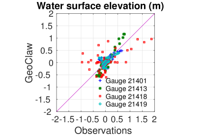
Prior to using these observations for the inference of the fault slip distribution, we verify the ability of GeoClaw to realistically simulate water surface elevation during the Tōhoku tsunami. To this end, we ran a single simulation of GeoClaw with default parameters and fault slip distribution from Ammon et al. [30] to predict the water surface elevation at the four gauges. We compare these with their DART counterparts and plot them in Figure 3 (Right) as a scatter plot for the gauges 21401, 21413, 21418 and 21419. The data points are colored differently for the different gauges and the variance of the difference between observations and simulations was calculated to be $7.99\times 10^{-3}~{}m^{2},9.65\times 10^{-3}~{}m^{2},4.62\times 10^{-2}~{}m^{2}$ and $5.86\times 10^{-3}~{}m^{2}$, respectively. These variances are consistent with the distance from the gauges to the epicenter of the earthquake located approximately 72 kilometers east of Japan. The smallest variance was at gauge 21419 (the farthest gauge from the epicenter) while the higher variance was at gauge 21418 that can be attributed to its proximity to the epicenter of the earthquake as well as to the shore region. The scatter plot along with the calculated variances indicate a reasonable agreement between the simulations and the observations at the different gauges. The overall differences between the simulations and observations can likely be attributed to uncertainties in the input data such as the Manning’s $n$ coefficients [1], fault slip distribution, errors in the earthquake rupture model, insufficiently accurate bathymetry in the near-shore region, and to model errors, such as unresolved effects and approximations inherent in the shallow water model.

3.2 Inverse problem

Bayesian inference is a well-established probabilistic approach to inverse problems in which all forms of uncertainty are expressed in terms of random variables. This method provides complete posterior statistics and not just a single value for the quantity of interest ($QoI$) [33]. Consider a set of $N$ water surface elevation observations ${\mathchoice{\mbox{\boldmath$\displaystyle{\eta}$}}{\mbox{\boldmath$\textstyle{\eta}$}}{\mbox{\boldmath$\scriptstyle{\eta}$}}{\mbox{\boldmath$\scriptscriptstyle{\eta}$}}}_{j}=\{{\eta}_{j}^{k}\}_{k=1}^{N}$ measured at the different DART buoy gauges $j=1,2,3$ and $4$, corresponding to gauges 21401, 21413, 21418 and 21419, respectively. Let ${\mathchoice{\mbox{\boldmath$\displaystyle{s}$}}{\mbox{\boldmath$\textstyle{s}$}}{\mbox{\boldmath$\scriptstyle{s}$}}{\mbox{\boldmath$\scriptscriptstyle{s}$}}}=\{s_{i}\}_{i=1}^{m=6}$ be a vector of uncertain parameters representing the six fault slip values. We consider the forward model ${\mathchoice{\mbox{\boldmath$\displaystyle{G}$}}{\mbox{\boldmath$\textstyle{G}$}}{\mbox{\boldmath$\scriptstyle{G}$}}{\mbox{\boldmath$\scriptscriptstyle{G}$}}}_{j}({\mathchoice{\mbox{\boldmath$\displaystyle{s}$}}{\mbox{\boldmath$\textstyle{s}$}}{\mbox{\boldmath$\scriptstyle{s}$}}{\mbox{\boldmath$\scriptscriptstyle{s}$}}})=\{{G}_{j}^{k}({\mathchoice{\mbox{\boldmath$\displaystyle{s}$}}{\mbox{\boldmath$\textstyle{s}$}}{\mbox{\boldmath$\scriptstyle{s}$}}{\mbox{\boldmath$\scriptscriptstyle{s}$}}})\}_{k=1}^{N}$ represented by GeoClaw that predicts the $N$ data at the $j^{th}$ gauge as a function of the vector of parameters $\textstyle{s}$ given observations ${\mathchoice{\mbox{\boldmath$\displaystyle{\eta}$}}{\mbox{\boldmath$\textstyle{\eta}$}}{\mbox{\boldmath$\scriptstyle{\eta}$}}{\mbox{\boldmath$\scriptscriptstyle{\eta}$}}}_{j}$. Bayes’s theorem can be applied that yields:

$$\pi({\mathchoice{\mbox{\boldmath$\displaystyle{s}$}}{\mbox{\boldmath$\textstyle{s}$}}{\mbox{\boldmath$\scriptstyle{s}$}}{\mbox{\boldmath$\scriptscriptstyle{s}$}}}|{{\mathchoice{\mbox{\boldmath$\displaystyle{\eta}$}}{\mbox{\boldmath$\textstyle{\eta}$}}{\mbox{\boldmath$\scriptstyle{\eta}$}}{\mbox{\boldmath$\scriptscriptstyle{\eta}$}}}}_{j})\propto\pi({{\mathchoice{\mbox{\boldmath$\displaystyle{\eta}$}}{\mbox{\boldmath$\textstyle{\eta}$}}{\mbox{\boldmath$\scriptstyle{\eta}$}}{\mbox{\boldmath$\scriptscriptstyle{\eta}$}}}}_{j}|{\mathchoice{\mbox{\boldmath$\displaystyle{s}$}}{\mbox{\boldmath$\textstyle{s}$}}{\mbox{\boldmath$\scriptstyle{s}$}}{\mbox{\boldmath$\scriptscriptstyle{s}$}}})\ \pi({\mathchoice{\mbox{\boldmath$\displaystyle{s}$}}{\mbox{\boldmath$\textstyle{s}$}}{\mbox{\boldmath$\scriptstyle{s}$}}{\mbox{\boldmath$\scriptscriptstyle{s}$}}}),$$ (2)

where $\pi({\mathchoice{\mbox{\boldmath$\displaystyle{s}$}}{\mbox{\boldmath$\textstyle{s}$}}{\mbox{\boldmath$\scriptstyle{s}$}}{\mbox{\boldmath$\scriptscriptstyle{s}$}}})$ is the prior of $\textstyle{s}$, $\pi({{\mathchoice{\mbox{\boldmath$\displaystyle{\eta}$}}{\mbox{\boldmath$\textstyle{\eta}$}}{\mbox{\boldmath$\scriptstyle{\eta}$}}{\mbox{\boldmath$\scriptscriptstyle{\eta}$}}}}_{j}|{\mathchoice{\mbox{\boldmath$\displaystyle{s}$}}{\mbox{\boldmath$\textstyle{s}$}}{\mbox{\boldmath$\scriptstyle{s}$}}{\mbox{\boldmath$\scriptscriptstyle{s}$}}})$ is the likelihood function and $\pi({\mathchoice{\mbox{\boldmath$\displaystyle{s}$}}{\mbox{\boldmath$\textstyle{s}$}}{\mbox{\boldmath$\scriptstyle{s}$}}{\mbox{\boldmath$\scriptscriptstyle{s}$}}}|{{\mathchoice{\mbox{\boldmath$\displaystyle{\eta}$}}{\mbox{\boldmath$\textstyle{\eta}$}}{\mbox{\boldmath$\scriptstyle{\eta}$}}{\mbox{\boldmath$\scriptscriptstyle{\eta}$}}}}_{j})$ is the posterior of $\textstyle{s}$. The likelihood function $L({\mathchoice{\mbox{\boldmath$\displaystyle{s}$}}{\mbox{\boldmath$\textstyle{s}$}}{\mbox{\boldmath$\scriptstyle{s}$}}{\mbox{\boldmath$\scriptscriptstyle{s}$}}}|{{\mathchoice{\mbox{\boldmath$\displaystyle{\eta}$}}{\mbox{\boldmath$\textstyle{\eta}$}}{\mbox{\boldmath$\scriptstyle{\eta}$}}{\mbox{\boldmath$\scriptscriptstyle{\eta}$}}}}_{j})=\pi({{\mathchoice{\mbox{\boldmath$\displaystyle{\eta}$}}{\mbox{\boldmath$\textstyle{\eta}$}}{\mbox{\boldmath$\scriptstyle{\eta}$}}{\mbox{\boldmath$\scriptscriptstyle{\eta}$}}}}_{j}|{\mathchoice{\mbox{\boldmath$\displaystyle{s}$}}{\mbox{\boldmath$\textstyle{s}$}}{\mbox{\boldmath$\scriptstyle{s}$}}{\mbox{\boldmath$\scriptscriptstyle{s}$}}})$ can be formulated assuming that independent additive errors account for the discrepancy between the predicted, ${\mathchoice{\mbox{\boldmath$\displaystyle{G}$}}{\mbox{\boldmath$\textstyle{G}$}}{\mbox{\boldmath$\scriptstyle{G}$}}{\mbox{\boldmath$\scriptscriptstyle{G}$}}}_{j}({\mathchoice{\mbox{\boldmath$\displaystyle{s}$}}{\mbox{\boldmath$\textstyle{s}$}}{\mbox{\boldmath$\scriptstyle{s}$}}{\mbox{\boldmath$\scriptscriptstyle{s}$}}})=\{{G}_{j}^{k}({\mathchoice{\mbox{\boldmath$\displaystyle{s}$}}{\mbox{\boldmath$\textstyle{s}$}}{\mbox{\boldmath$\scriptstyle{s}$}}{\mbox{\boldmath$\scriptscriptstyle{s}$}}})\}_{k=1}^{N}$, and observed ${\mathchoice{\mbox{\boldmath$\displaystyle{\eta}$}}{\mbox{\boldmath$\textstyle{\eta}$}}{\mbox{\boldmath$\scriptstyle{\eta}$}}{\mbox{\boldmath$\scriptscriptstyle{\eta}$}}}_{j}=\{{\eta}_{j}^{k}\}_{k=1}^{N}$, values of water surface elevation such that:

$${\epsilon}_{j}^{k}={G}_{j}^{k}({\mathchoice{\mbox{\boldmath$\displaystyle{s}$}}{\mbox{\boldmath$\textstyle{s}$}}{\mbox{\boldmath$\scriptstyle{s}$}}{\mbox{\boldmath$\scriptscriptstyle{s}$}}})-{\eta}_{j}^{k},\quad j=1\ldots 4,\quad k=1\ldots N,$$

where ${{\mathchoice{\mbox{\boldmath$\displaystyle{\epsilon}$}}{\mbox{\boldmath$\textstyle{\epsilon}$}}{\mbox{\boldmath$\scriptstyle{\epsilon}$}}{\mbox{\boldmath$\scriptscriptstyle{\epsilon}$}}}}_{j}=\{{\epsilon}_{j}^{k}\}_{k=1}^{N}$ are assumed to be i.i.d. random variables with density $p_{\epsilon_{j}}$. The likelihood function can then be written as

$$L({\mathchoice{\mbox{\boldmath$\displaystyle{s}$}}{\mbox{\boldmath$\textstyle{s}$}}{\mbox{\boldmath$\scriptstyle{s}$}}{\mbox{\boldmath$\scriptscriptstyle{s}$}}}|{{\mathchoice{\mbox{\boldmath$\displaystyle{\eta}$}}{\mbox{\boldmath$\textstyle{\eta}$}}{\mbox{\boldmath$\scriptstyle{\eta}$}}{\mbox{\boldmath$\scriptscriptstyle{\eta}$}}}}_{j})=\prod_{j=1}^{4}\prod_{k=1}^{N}p_{\epsilon_{j}}(G_{j}^{k}({\mathchoice{\mbox{\boldmath$\displaystyle{s}$}}{\mbox{\boldmath$\textstyle{s}$}}{\mbox{\boldmath$\scriptstyle{s}$}}{\mbox{\boldmath$\scriptscriptstyle{s}$}}})-{\eta}_{j}^{k}).$$ (3)

In our application, the measurements may vary significantly from one gauge to another and the observations collected may be exposed to different measurement errors; therefore, it is reasonable to assume that the errors are normally distributed with zero mean and a variance that depends on location, i.e.  $\epsilon_{j}^{k}\sim N(0,\sigma_{j}^{2})$ where $\sigma_{j}^{2}$ ($j=1\ldots 4$) is the variance at the different gauges. Thus the likelihood function can be expressed as

$$L({\mathchoice{\mbox{\boldmath$\displaystyle{s}$}}{\mbox{\boldmath$\textstyle{s}$}}{\mbox{\boldmath$\scriptstyle{s}$}}{\mbox{\boldmath$\scriptscriptstyle{s}$}}}|{{\mathchoice{\mbox{\boldmath$\displaystyle{\eta}$}}{\mbox{\boldmath$\textstyle{\eta}$}}{\mbox{\boldmath$\scriptstyle{\eta}$}}{\mbox{\boldmath$\scriptscriptstyle{\eta}$}}}}_{j})=\prod_{j=1}^{4}\prod_{k=1}^{N}\frac{1}{\sqrt{2\pi\sigma_{j}^{2}}}\exp\left\{\frac{-(G_{j}^{k}({\mathchoice{\mbox{\boldmath$\displaystyle{s}$}}{\mbox{\boldmath$\textstyle{s}$}}{\mbox{\boldmath$\scriptstyle{s}$}}{\mbox{\boldmath$\scriptscriptstyle{s}$}}})-\eta^{k}_{j})^{2}}{2\sigma_{j}^{2}}\right\},$$ (4)

and the joint posterior in Equation 2 becomes

$$\pi({\mathchoice{\mbox{\boldmath$\displaystyle{s}$}}{\mbox{\boldmath$\textstyle{s}$}}{\mbox{\boldmath$\scriptstyle{s}$}}{\mbox{\boldmath$\scriptscriptstyle{s}$}}}|\eta^{k}_{j})\propto\prod_{j=1}^{4}\prod_{k=1}^{N}\frac{1}{\sqrt{2\pi\sigma_{j}^{2}}}\exp\left\{\frac{-(G_{j}^{k}({\mathchoice{\mbox{\boldmath$\displaystyle{s}$}}{\mbox{\boldmath$\textstyle{s}$}}{\mbox{\boldmath$\scriptstyle{s}$}}{\mbox{\boldmath$\scriptscriptstyle{s}$}}})-\eta^{k}_{j})^{2}}{2\sigma_{j}^{2}}\right\}\prod_{i=1}^{6}\pi(s_{i}).$$

The variance $\sigma_{j}^{2}$ is not well known a priori, thus it is treated as a hyper-parameter that becomes an additional parameter for Bayesian inference endowed with a prior which is updated based on available observations. In this case the joint posterior is finally expressed as

$$\pi(s_{i},\sigma_{j}^{2}|\eta_{j}^{k})\propto\prod_{j=1}^{4}\prod_{k=1}^{N}\frac{1}{\sqrt{2\pi\sigma_{j}^{2}}}\exp\left\{\frac{-(G_{j}^{k}({\mathchoice{\mbox{\boldmath$\displaystyle{s}$}}{\mbox{\boldmath$\textstyle{s}$}}{\mbox{\boldmath$\scriptstyle{s}$}}{\mbox{\boldmath$\scriptscriptstyle{s}$}}})-\eta^{k}_{j})^{2}}{2\sigma_{k}^{2}}\right\}\ \prod_{i=1}^{6}\pi(s_{i})\prod_{j=1}^{4}\pi(\sigma_{j}^{2}).$$ (5)

Finally, proper priors are chosen for the uncertain parameters based on some a priori knowledge about them. In our case, we chose a non-informative uniform prior for all six fault slip values, with $s_{i}$ in the range $[s_{min}-s_{max}]$ so that $\pi(s_{i})=\frac{1}{s_{max}-s_{min}}$. Regarding the noise variance, the only information known is that $\sigma_{j}^{2}$ is always positive. We thus assume a Jeffreys prior [34] for $\sigma_{j}^{2}$, expressed as:

$$\pi(\sigma_{j}^{2})=\begin{cases}\displaystyle\frac{1}{\sigma_{j}^{2}}&\text{for~{}}\sigma_{j}^{2}>0,\\ 0&\text{otherwise}.\end{cases}$$ (6)

The described Bayesian formulation requires sampling the resulting posterior (Equation 5) to estimate the joint posterior of the parameters. Markov Chain Monte Carlo (MCMC) methods are convenient and popular sampling strategies that require a large number of posterior evaluations. We rely on an adaptive Metropolis MCMC algorithm  [35, 36] to efficiently sample the posterior distribution. In addition, we build a surrogate model of the model response for further reduction in computational time as explained below.

3.3 Surrogate model

To accelerate the process of sampling the posterior (Equation 5) using MCMC, we build a surrogate model of the $QoIs$, namely the ${\mathchoice{\mbox{\boldmath$\displaystyle{\eta}$}}{\mbox{\boldmath$\textstyle{\eta}$}}{\mbox{\boldmath$\scriptstyle{\eta}$}}{\mbox{\boldmath$\scriptscriptstyle{\eta}$}}}_{j}$’s using a small ensemble of GeoClaw model runs. For this purpose, we apply a probabilistic method to express the $QoI$ as a function of the uncertain model inputs, namely the Polynomial Chaos (PC) method [24, 37]. As the name indicates, the function would be in the form of a polynomial expansion [38, 37] that is truncated at a specific order. This approach was adopted in [1] to build a surrogate model for the water surface elevation and then used to determine statistical properties (mean and variance) as well as sensitivities [39]. Additionally the surrogate model was used for efficient sampling of the posteriors. We briefly show here the process of constructing a PC surrogate for the $QoI$; for more details on the PC method the reader is referred to [24].

3.3.1 Polynomial Chaos

We denote by $G=G({\mathchoice{\mbox{\boldmath$\displaystyle{\xi}$}}{\mbox{\boldmath$\textstyle{\xi}$}}{\mbox{\boldmath$\scriptstyle{\xi}$}}{\mbox{\boldmath$\scriptscriptstyle{\xi}$}}})$ our $QoI$ which is the water surface elevation produced by GeoClaw; ${\mathchoice{\mbox{\boldmath$\displaystyle{\xi}$}}{\mbox{\boldmath$\textstyle{\xi}$}}{\mbox{\boldmath$\scriptstyle{\xi}$}}{\mbox{\boldmath$\scriptscriptstyle{\xi}$}}}=[\xi_{1},...,\xi_{m}]$ denotes the canonical vector of $m$ random variables that parameterize the uncertain fault slip values as follows:

$$\xi_{i}=\frac{2s_{i}-(s_{min}+s_{min})}{(s_{min}-s_{max})}.$$

The PC method seeks to represent $G$ as a function of the uncertain input variables $\textstyle{\xi}$ as

$$G({\mathchoice{\mbox{\boldmath$\displaystyle{\xi}$}}{\mbox{\boldmath$\textstyle{\xi}$}}{\mbox{\boldmath$\scriptstyle{\xi}$}}{\mbox{\boldmath$\scriptscriptstyle{\xi}$}}})\approx\sum_{k=0}^{R}g_{k}\psi_{k}({\mathchoice{\mbox{\boldmath$\displaystyle{\xi}$}}{\mbox{\boldmath$\textstyle{\xi}$}}{\mbox{\boldmath$\scriptstyle{\xi}$}}{\mbox{\boldmath$\scriptscriptstyle{\xi}$}}}),$$ (7)

where $g_{k}$ are the polynomial coefficients to be determined, and $\psi_{k}({\mathchoice{\mbox{\boldmath$\displaystyle{\xi}$}}{\mbox{\boldmath$\textstyle{\xi}$}}{\mbox{\boldmath$\scriptstyle{\xi}$}}{\mbox{\boldmath$\scriptscriptstyle{\xi}$}}})$ are tensor products of the scaled Legendre polynomials [24] forming an orthogonal basis of the space of square integrable functions of the underlying uniform probability distributions $\rho({\mathchoice{\mbox{\boldmath$\displaystyle{\xi}$}}{\mbox{\boldmath$\textstyle{\xi}$}}{\mbox{\boldmath$\scriptstyle{\xi}$}}{\mbox{\boldmath$\scriptscriptstyle{\xi}$}}})$ with

$$\left<\psi_{i},\psi_{j}\right>=\int\psi_{i}({\mathchoice{\mbox{\boldmath$\displaystyle{\xi}$}}{\mbox{\boldmath$\textstyle{\xi}$}}{\mbox{\boldmath$\scriptstyle{\xi}$}}{\mbox{\boldmath$\scriptscriptstyle{\xi}$}}})\;\psi_{j}({\mathchoice{\mbox{\boldmath$\displaystyle{\xi}$}}{\mbox{\boldmath$\textstyle{\xi}$}}{\mbox{\boldmath$\scriptstyle{\xi}$}}{\mbox{\boldmath$\scriptscriptstyle{\xi}$}}})\;\rho({\mathchoice{\mbox{\boldmath$\displaystyle{\xi}$}}{\mbox{\boldmath$\textstyle{\xi}$}}{\mbox{\boldmath$\scriptstyle{\xi}$}}{\mbox{\boldmath$\scriptscriptstyle{\xi}$}}})\;\mbox{d}{\mathchoice{\mbox{\boldmath$\displaystyle{\xi}$}}{\mbox{\boldmath$\textstyle{\xi}$}}{\mbox{\boldmath$\scriptstyle{\xi}$}}{\mbox{\boldmath$\scriptscriptstyle{\xi}$}}}=\delta_{ij}\left\langle{\psi_{i}^{2}}\right\rangle,$$ (8)

The PC coefficients $g_{k}$ can be determined using a number of methods. In this work, we rely on non-intrusive approaches [40, 15] that use a set of deterministic model runs $G({\mathchoice{\mbox{\boldmath$\displaystyle{\xi}$}}{\mbox{\boldmath$\textstyle{\xi}$}}{\mbox{\boldmath$\scriptstyle{\xi}$}}{\mbox{\boldmath$\scriptscriptstyle{\xi}$}}})$ evaluated at particular realizations of $\textstyle{\xi}$. In particular, we relied on two non-intrusive methods described in Section 3.3.2 and Section 3.3.3 below. The reasoning behind using these two methods is explained in the results section.

3.3.2 Non-Intrusive Spectral Projection

The Non-Intrusive Spectral Projection (NISP) method makes use of the orthogonality of the polynomial basis and applies a Galerkin projection to find the PC expansion coefficients [41, 42] as

$$g_{k}=\frac{\left<G,\psi_{k}\right>}{\left<\psi_{k},\psi_{k}\right>}=\frac{1}{\left<\psi_{k},\psi_{k}\right>}\int G\psi_{k}({\mathchoice{\mbox{\boldmath$\displaystyle{\xi}$}}{\mbox{\boldmath$\textstyle{\xi}$}}{\mbox{\boldmath$\scriptstyle{\xi}$}}{\mbox{\boldmath$\scriptscriptstyle{\xi}$}}})\rho({\mathchoice{\mbox{\boldmath$\displaystyle{\xi}$}}{\mbox{\boldmath$\textstyle{\xi}$}}{\mbox{\boldmath$\scriptstyle{\xi}$}}{\mbox{\boldmath$\scriptscriptstyle{\xi}$}}})\mbox{ d}{\mathchoice{\mbox{\boldmath$\displaystyle{\xi}$}}{\mbox{\boldmath$\textstyle{\xi}$}}{\mbox{\boldmath$\scriptstyle{\xi}$}}{\mbox{\boldmath$\scriptscriptstyle{\xi}$}}}.$$

A numerical quadrature is used to approximate the integrals with

$$\int G\psi_{k}({\mathchoice{\mbox{\boldmath$\displaystyle{\xi}$}}{\mbox{\boldmath$\textstyle{\xi}$}}{\mbox{\boldmath$\scriptstyle{\xi}$}}{\mbox{\boldmath$\scriptscriptstyle{\xi}$}}})\rho({\mathchoice{\mbox{\boldmath$\displaystyle{\xi}$}}{\mbox{\boldmath$\textstyle{\xi}$}}{\mbox{\boldmath$\scriptstyle{\xi}$}}{\mbox{\boldmath$\scriptscriptstyle{\xi}$}}})\mbox{ d}{\mathchoice{\mbox{\boldmath$\displaystyle{\xi}$}}{\mbox{\boldmath$\textstyle{\xi}$}}{\mbox{\boldmath$\scriptstyle{\xi}$}}{\mbox{\boldmath$\scriptscriptstyle{\xi}$}}}\approx\sum_{q=1}^{Q}G({\mathchoice{\mbox{\boldmath$\displaystyle{\xi}$}}{\mbox{\boldmath$\textstyle{\xi}$}}{\mbox{\boldmath$\scriptstyle{\xi}$}}{\mbox{\boldmath$\scriptscriptstyle{\xi}$}}}_{q})\psi_{k}({\mathchoice{\mbox{\boldmath$\displaystyle{\xi}$}}{\mbox{\boldmath$\textstyle{\xi}$}}{\mbox{\boldmath$\scriptstyle{\xi}$}}{\mbox{\boldmath$\scriptscriptstyle{\xi}$}}}_{q})\omega_{q},$$

where ${\mathchoice{\mbox{\boldmath$\displaystyle{\xi}$}}{\mbox{\boldmath$\textstyle{\xi}$}}{\mbox{\boldmath$\scriptstyle{\xi}$}}{\mbox{\boldmath$\scriptscriptstyle{\xi}$}}}_{q}$ and $\omega_{q}$ are the multi-dimensional quadrature points and weights, respectively, and $Q$ is the total number of nodes in the multi-dimensional quadrature. $G({\mathchoice{\mbox{\boldmath$\displaystyle{\xi}$}}{\mbox{\boldmath$\textstyle{\xi}$}}{\mbox{\boldmath$\scriptstyle{\xi}$}}{\mbox{\boldmath$\scriptscriptstyle{\xi}$}}}_{q})$ is the model prediction evaluated at the quadrature values ${\mathchoice{\mbox{\boldmath$\displaystyle{\xi}$}}{\mbox{\boldmath$\textstyle{\xi}$}}{\mbox{\boldmath$\scriptstyle{\xi}$}}{\mbox{\boldmath$\scriptscriptstyle{\xi}$}}}_{q}$. We note that the order of quadrature should be commensurated with the PC truncation order, and should be high enough to avoid aliasing artifacts.

3.3.3 Basis-Pursuit DeNoising

Basis-Pursuit DeNoising (BPDN) is a non-intrusive method for finding the PC coefficients using a number of random model evaluations. BPDN is based on the compressed sensing methodology that assumes sparsity in a signal, in our case the PC coefficients, and seeks to determine the non-zero coefficients. using optimization techniques [40, 43, 19]. Let ${{\mathchoice{\mbox{\boldmath$\displaystyle{g}$}}{\mbox{\boldmath$\textstyle{g}$}}{\mbox{\boldmath$\scriptstyle{g}$}}{\mbox{\boldmath$\scriptscriptstyle{g}$}}}}=[g_{0},...,g_{R}]$ be the vector of PC coefficients to be determined and ${\mathchoice{\mbox{\boldmath$\displaystyle{G}$}}{\mbox{\boldmath$\textstyle{G}$}}{\mbox{\boldmath$\scriptstyle{G}$}}{\mbox{\boldmath$\scriptscriptstyle{G}$}}}=[G({\mathchoice{\mbox{\boldmath$\displaystyle{\xi}$}}{\mbox{\boldmath$\textstyle{\xi}$}}{\mbox{\boldmath$\scriptstyle{\xi}$}}{\mbox{\boldmath$\scriptscriptstyle{\xi}$}}}_{1}),...,G({\mathchoice{\mbox{\boldmath$\displaystyle{\xi}$}}{\mbox{\boldmath$\textstyle{\xi}$}}{\mbox{\boldmath$\scriptstyle{\xi}$}}{\mbox{\boldmath$\scriptscriptstyle{\xi}$}}}_{S})]$ be the vector of random model evaluations at the sampled ${\mathchoice{\mbox{\boldmath$\displaystyle{\xi}$}}{\mbox{\boldmath$\textstyle{\xi}$}}{\mbox{\boldmath$\scriptstyle{\xi}$}}{\mbox{\boldmath$\scriptscriptstyle{\xi}$}}}_{s}$. We also let $\Psi$ be a matrix whose rows are evaluations of the PC basis functions $\psi_{k}({\mathchoice{\mbox{\boldmath$\displaystyle{\xi}$}}{\mbox{\boldmath$\textstyle{\xi}$}}{\mbox{\boldmath$\scriptstyle{\xi}$}}{\mbox{\boldmath$\scriptscriptstyle{\xi}$}}})$ at the sampled ${\mathchoice{\mbox{\boldmath$\displaystyle{\xi}$}}{\mbox{\boldmath$\textstyle{\xi}$}}{\mbox{\boldmath$\scriptstyle{\xi}$}}{\mbox{\boldmath$\scriptscriptstyle{\xi}$}}}_{s}$. We therefore transform Equation 7 into the following system in matrix form to solve for:

$${\mathchoice{\mbox{\boldmath$\displaystyle{G}$}}{\mbox{\boldmath$\textstyle{G}$}}{\mbox{\boldmath$\scriptstyle{G}$}}{\mbox{\boldmath$\scriptscriptstyle{G}$}}}=\Psi{\mathchoice{\mbox{\boldmath$\displaystyle{g}$}}{\mbox{\boldmath$\textstyle{g}$}}{\mbox{\boldmath$\scriptstyle{g}$}}{\mbox{\boldmath$\scriptscriptstyle{g}$}}}.$$

The sparsity in the system is exploited by constraining the system and minimizing its ”energy”, which is its $\ell_{1}$-norm, and thus solving the optimization problem

$${\cal{O}}_{1,\delta}\approx\left\{\arg\!\min_{{{\mathchoice{\mbox{\boldmath$\displaystyle{g}$}}{\mbox{\boldmath$\textstyle{g}$}}{\mbox{\boldmath$\scriptstyle{g}$}}{\mbox{\boldmath$\scriptscriptstyle{g}$}}}}}||{{\mathchoice{\mbox{\boldmath$\displaystyle{g}$}}{\mbox{\boldmath$\textstyle{g}$}}{\mbox{\boldmath$\scriptstyle{g}$}}{\mbox{\boldmath$\scriptscriptstyle{g}$}}}}||_{1}:||{\mathchoice{\mbox{\boldmath$\displaystyle{G}$}}{\mbox{\boldmath$\textstyle{G}$}}{\mbox{\boldmath$\scriptstyle{G}$}}{\mbox{\boldmath$\scriptscriptstyle{G}$}}}-\Psi{\mathchoice{\mbox{\boldmath$\displaystyle{g}$}}{\mbox{\boldmath$\textstyle{g}$}}{\mbox{\boldmath$\scriptstyle{g}$}}{\mbox{\boldmath$\scriptscriptstyle{g}$}}}||_{2}\leq\delta\right\}.$$ (9)

In this specific method, we assumed the presence of noise $\delta$ in the signal that is estimated a priori in contrast to the Basis-Pursuit (BP) technique where no noise is assumed [44]. The noise $\delta$ is determined using a cross-validation method that assures the computed PC coefficients not only fit the random model evaluations but also accurately approximate the model [19]. The system ${\cal{O}}_{1,\delta}$ is then solved using standard $\ell_{1}$-minimization solvers such as the MATLAB package SPGL1 [45], that is based on the spectral projected gradient algorithm [46].

4 Results

4.1 PC Expansion Construction and Validation

The construction of the PC surrogate for the water surface elevation using non-intrusive methods requires an ensemble of forward model runs. The shape (distribution) of the ensemble and number of members (model runs) is dictated by the particular method employed. In this work, we employ two different methods that require two different ensembles as follows:

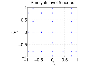
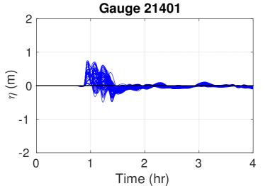
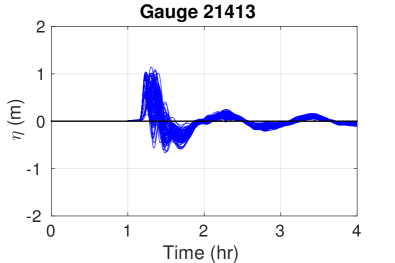
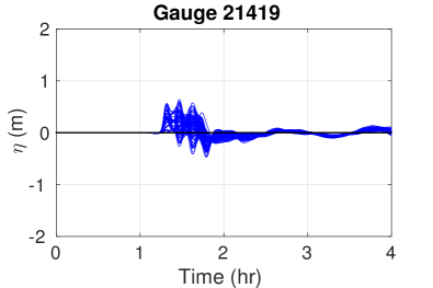
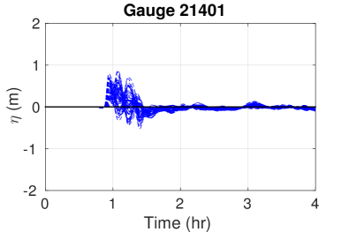
1. NISP requires a quadrature to compute the PC coefficients [1]. Here, we adopted a sparse nested Smolyak quadrature [47, 48, 49]. In particular, Smolyak level 5 grid rule was used requiring a total number of $Q=1889$ quadrature nodes for the case of $m=6$ uncertain parameters to accurately approximate PC expansion of order $p=5$. A two-dimensional projection of the quadrature grid is shown in Figure 4 (Left) on the ${\mathchoice{\mbox{\boldmath$\displaystyle{\xi}$}}{\mbox{\boldmath$\textstyle{\xi}$}}{\mbox{\boldmath$\scriptstyle{\xi}$}}{\mbox{\boldmath$\scriptscriptstyle{\xi}$}}}_{1}-{\mathchoice{\mbox{\boldmath$\displaystyle{\xi}$}}{\mbox{\boldmath$\textstyle{\xi}$}}{\mbox{\boldmath$\scriptstyle{\xi}$}}{\mbox{\boldmath$\scriptscriptstyle{\xi}$}}}_{2}$ plane. The evolution of the water surface elevation predicted by GeoClaw at these nodes is shown in Figure 5 at the four different gauges.

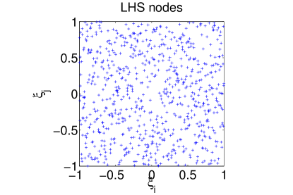
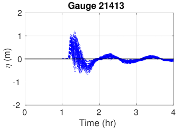
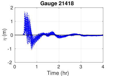
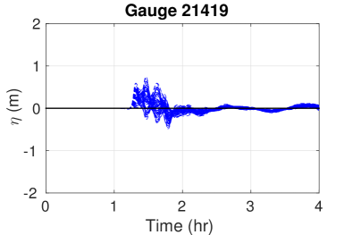
2. BPDN accommodates both regular and random sampling to determine the PC coefficients. Here, we used a Latin-Hyper-Cube (LHS) sample consisting of 729 GeoClaw realizations whose nodes are shown in Figure 4 (Right) when projected on the ${\mathchoice{\mbox{\boldmath$\displaystyle{\xi}$}}{\mbox{\boldmath$\textstyle{\xi}$}}{\mbox{\boldmath$\scriptstyle{\xi}$}}{\mbox{\boldmath$\scriptscriptstyle{\xi}$}}}_{1}-{\mathchoice{\mbox{\boldmath$\displaystyle{\xi}$}}{\mbox{\boldmath$\textstyle{\xi}$}}{\mbox{\boldmath$\scriptstyle{\xi}$}}{\mbox{\boldmath$\scriptscriptstyle{\xi}$}}}_{2}$ plane. The evolution of the water surface elevation predicted by GeoClaw at these nodes is shown in Figure 6 at the four different gauges.

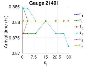
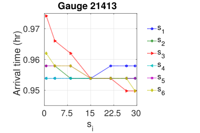
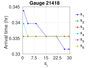
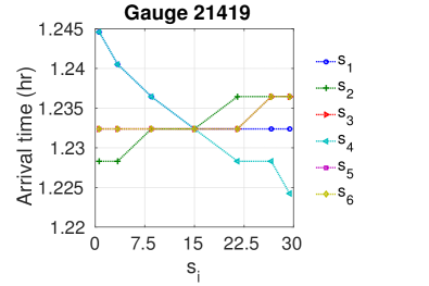
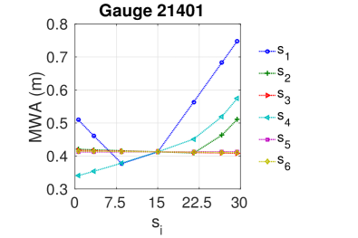
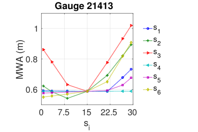
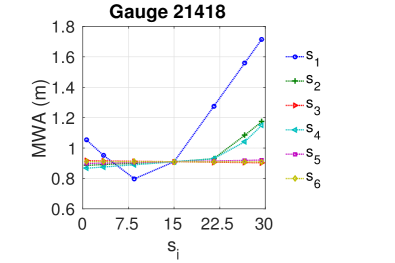
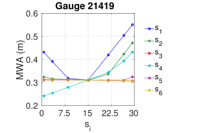
In both sets of realizations, we notice that the variability in water surface elevation is significant at all gauges. This variability in the prediction of water surface elevation persists till the end of the simulations for all gauges as well. It is noticed that this variability is present in the arrival time in addition to the Maximum Wave Amplitude (MWA). To confirm, we estimate the arrival time and MWA of the 1889 realizations corresponding to the quadrature sample and plot them as functions of the different slip values $s_{i}$ on the subfaults (other values are set to $s_{j}=15$) in Figure 7 and Figure 8, respectively. We clearly notice the significant variation of arrival time with the slip values and similarly for the MWA. These variations are expected to be challenging when computing the PC coefficients as it might require a high order PC expansion [50].

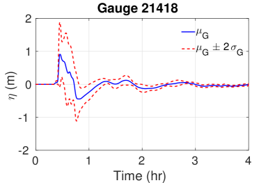
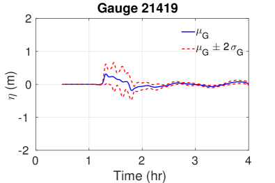
Finally, we note that the average arrival time and average MWA are both consistent with the distance from the gauge to the epicenter of the earthquake (located approximately 72 kilometer east of Japan). For instance, gauge 21418 is the closest to the source as shown in Figure 1 with the shortest arrival time and largest MWA, while on the other hand, gauge 21419 is the farthest from the source with the longest arrival time and smallest MWA.

4.1.1 Non-Intrusive Spectral Projection

The PC expansion coefficients are first computed using the output of the 1889 quadrature ensemble. The constructed PC surrogate is validated using the normalized relative error (NRE) that measures the accuracy of predicted values by the PC surrogate using an independent set of GeoClaw simulations as follows:

$$NRE=\frac{\displaystyle\left(\sum_{q=1}^{S}\left|G({\mathchoice{\mbox{\boldmath$\displaystyle{\xi}$}}{\mbox{\boldmath$\textstyle{\xi}$}}{\mbox{\boldmath$\scriptstyle{\xi}$}}{\mbox{\boldmath$\scriptscriptstyle{\xi}$}}}_{s})-\sum_{k=0}^{R}g_{k}\psi_{k}({\mathchoice{\mbox{\boldmath$\displaystyle{\xi}$}}{\mbox{\boldmath$\textstyle{\xi}$}}{\mbox{\boldmath$\scriptstyle{\xi}$}}{\mbox{\boldmath$\scriptscriptstyle{\xi}$}}}_{q})\right|^{2}\right)^{1/2}}{\displaystyle\left(\sum_{q=1}^{S}\left|G({\mathchoice{\mbox{\boldmath$\displaystyle{\xi}$}}{\mbox{\boldmath$\textstyle{\xi}$}}{\mbox{\boldmath$\scriptstyle{\xi}$}}{\mbox{\boldmath$\scriptscriptstyle{\xi}$}}}_{s})\right|^{2}\right)^{1/2}},$$ (10)

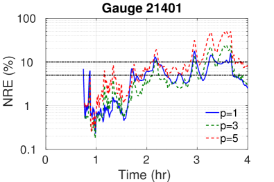
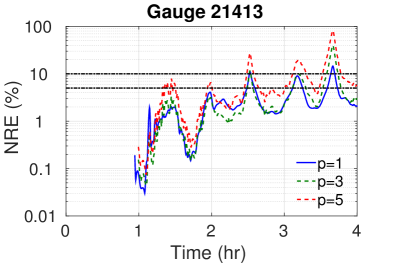
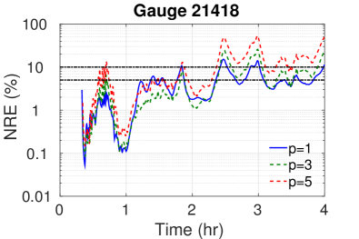
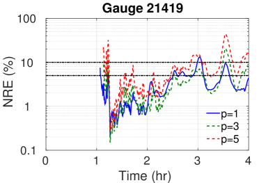
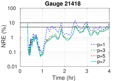
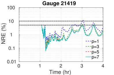
where $G({\mathchoice{\mbox{\boldmath$\displaystyle{\xi}$}}{\mbox{\boldmath$\textstyle{\xi}$}}{\mbox{\boldmath$\scriptstyle{\xi}$}}{\mbox{\boldmath$\scriptscriptstyle{\xi}$}}}_{s})$ is the $QoI$ corresponding to the LHS sample that were not used in the PC construction process. The evolution of NRE is shown in Figure 9 for different PC orders as indicated. The horizontal dotted lines are guides to the eye indicating the $5\%$ and $10\%$ errors. The calculated NRE appears to be larger than $10\%$ for PC order $p=1$ at certain times that amplifies with increasing PC order. This indicates convergence issues in the PC that leads to inaccuracies in the representation of the $QoI$. This is noticed for all the gauges.

We conclude that the construction of a converging PC expansion using the NISP method was not successful which promoted us to use an to alternative method. The large errors can be attributed to the large variation in the arrival times and the MWA that is not tolerated by the NISP method. One option to overcome this issue is preconditioning the $QoI$. This idea was proposed in [51, 16], where appropriate transformations of the original time-dependent $QoI$ into a new one having a tight sparse PC expansion, thus requiring less effort to be projected. Instead we resort here to a recent compressed technique as explained above.

4.1.2 Basis-Pursuit DeNoising

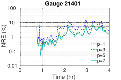
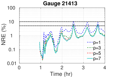
We next applied the BPDN method to estimate the PC coefficients [19] using the LHS sample consisting of 729 GeoClaw realizations. We again quantified the agreement between the PC surrogate and the GeoClaw realizations where we now calculate the NRE using the Smolyak quadrature sample (not used in the PC coefficients estimation). The evolution of error shown in Figure 10 indicate a better agreement (compared to NISP) whereas the maximum error was found to decrease as the PC order is increased. The average error is less than $5\%$, indicating that BPDN is successful in constructing a surrogate that yields accurate $QoI$ predictions.

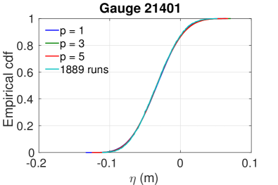
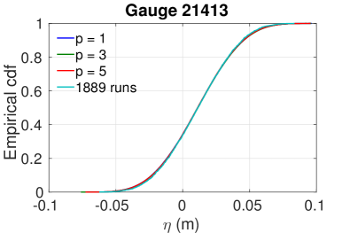
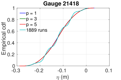
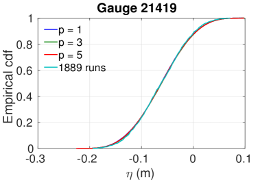
We also computed the empirical CDF of water surface elevation at the different gauges using samples from the PC surrogate for different orders. We also computed the CDF using the 1889 GeoClaw model runs and compare them to the PC-estimated ones and plot them in Figure 11. These different panel show that the CDFs obtained using higher order bases agree with each other and with the CDF obtained from the full model runs directly.

In conclusion, these tests provide confidence that the PC expansion is a faithful model surrogate that can be used in both the forward and inverse problems.

4.2 Statistical Analysis

The PC expansion created using an ensemble of GeoClaw simulations simplifies the calculations of the statistical moments of model output $G$ as the expectation and variance can be computed from the PC coefficients as follows:

$$\mu_{G}=\int G\,\rho({\mathchoice{\mbox{\boldmath$\displaystyle{\xi}$}}{\mbox{\boldmath$\textstyle{\xi}$}}{\mbox{\boldmath$\scriptstyle{\xi}$}}{\mbox{\boldmath$\scriptscriptstyle{\xi}$}}})\,\mbox{d}{\mathchoice{\mbox{\boldmath$\displaystyle{\xi}$}}{\mbox{\boldmath$\textstyle{\xi}$}}{\mbox{\boldmath$\scriptstyle{\xi}$}}{\mbox{\boldmath$\scriptscriptstyle{\xi}$}}}\approx\left<G,\psi_{0}\right>_{\cal Q}=G_{0},$$ (11)

$$\sigma^{2}_{G}=\int(G-\mu_{G})^{2}\,\rho({\mathchoice{\mbox{\boldmath$\displaystyle{\xi}$}}{\mbox{\boldmath$\textstyle{\xi}$}}{\mbox{\boldmath$\scriptstyle{\xi}$}}{\mbox{\boldmath$\scriptscriptstyle{\xi}$}}})\,\mbox{d}{\mathchoice{\mbox{\boldmath$\displaystyle{\xi}$}}{\mbox{\boldmath$\textstyle{\xi}$}}{\mbox{\boldmath$\scriptstyle{\xi}$}}{\mbox{\boldmath$\scriptscriptstyle{\xi}$}}}\approx\sum_{k=1}^{R}G_{k}^{2}\left<\psi_{k},\psi_{k}\right>.$$ (12)

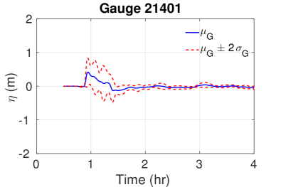
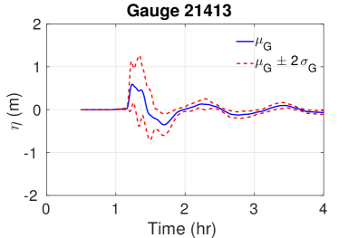
The evolution of the mean of the sea-surface elevation $\mu_{G}$ along with two standard deviation bounds ($\pm 2\sigma_{G}$) are thus computed from the PC coefficients and plotted in Figure 12 at the four gauges. Note that the evolution shown starts at $t=2hrs$ when the uncertainty becomes significant. An interesting observation is that the standard deviation in water surface elevations waxes and wanes as the tsunami evolves. The narrowing of the variance at these instances is possibly associated with the waves that arrive due to reflections from a single source and then move away from the gauge location imposing no variance in the water surface elevation.

4.3 Fault Slip Inference

Finally with our PC surrogate in hand we can solve the inverse problem, estimating the fault slip values as well as the variance of the noise in the measured data using Bayesian inference. For this purpose, we implement an adaptive MCMC method  [36, 35] to sample the posterior distributions in Equation 5 and consequently update the uncertain parameters.

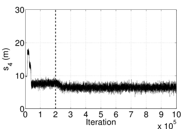
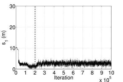
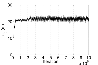
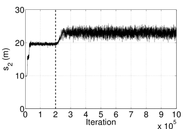
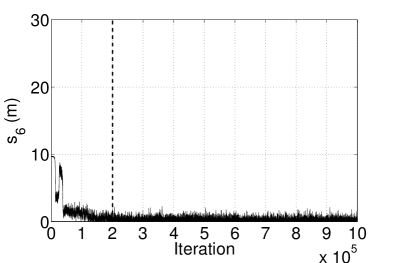
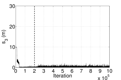
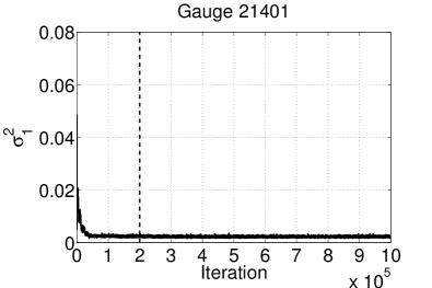
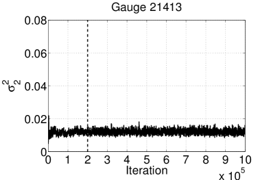
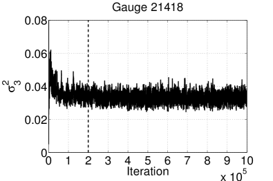
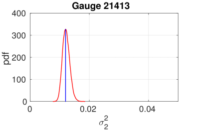
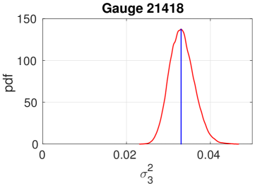
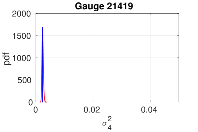
The posterior was sampled $10^{6}$ times after which we find negligible change in the estimated posteriors of the fault slip values: $s_{1}\ldots s_{6}$ as well as for the noise variance $\sigma^{2}_{1}\ldots\sigma^{2}_{4}$ with further iterations. Figure 13 plots the sample chains for the input parameters for different iterations of the MCMC algorithm. The different panels show well-mixed chains for all input parameters where the chains of $s_{1},s_{2},s_{4}$ and $s_{5}$ appear to be concentrated in an area of the parameter prior range. In contrast, the $s_{3}$ and $s_{6}$ chains appear to be concentrated in the lower end of the parameter range. The running mean plotted in Figure 14 is an indication of the convergence of the MCMC. The chains for the noise variances ($\sigma^{2}_{1}\ldots\sigma^{2}_{4}$) are shown in Figure 15 at the different gauges and appear to be well mixed with a well defined posterior range. The maximum variance appears to be at gauge 21418 and its range lies between 0.025 and 0.045.

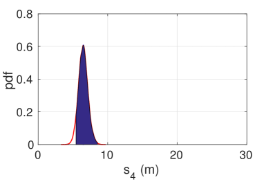
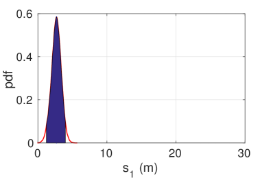
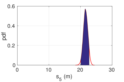
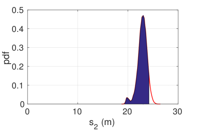
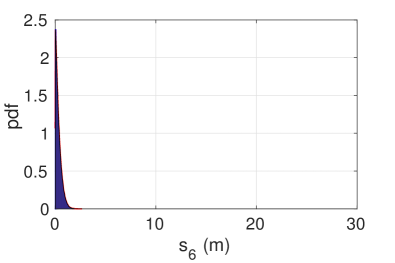
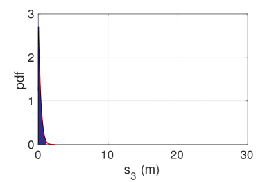
We used Kernel Density Estimation (KDE) [53, 54] to determine the marginalized posterior probability distribution functions (pdfs) using the computed MCMC chains and plot them in Figure 16 for the different parameters. The first $2\times 10^{5}$ MCMC iterations were considered as the burn-in period and thus discarded. The shapes of the marginalized posterior pdfs are consistent with the chains shown in Figure 13 where the pdfs of $s_{1},s_{2},s_{4}$ and $s_{5}$ appear to have a Gaussian-like shape with a well-defined peak; the Maximum A Posteriori (MAP) values are estimated to be $2.7,~{}23,~{}6.5$ and $21.5$ respectively. On the other hand, for $s_{3}$ and $s_{6}$ and the pdfs exhibit also a well-defined peak, but with an extended tail towards the smaller slip values; the mean values are estimated to be $0.3$ for both. The 95% intervals of high posterior probability are shown as shaded regions for the inferred parameters.

Regarding the noise variances, their pdfs are shown in Figure 17 at the different gauges. The pdfs appear to be well-defined and Gaussian shaped with a clear MAP values. These MAP values can be used to estimate the maximum water surface elevation standard deviation that was found to be $\sigma_{3}=0.182~{}m$ at gauge 21418. This value is a reflection of the mismatch between the model and observed data. The $\sigma^{2}_{i}$ estimates are noticeably lower than those obtained with GeoClaw default slip distribution (shown in Figure 3 (Right)): $2.27\times 10^{-3}~{}m^{2}$ versus $7.99\times 10^{-3}~{}m^{2}$, $1.22\times 10^{-2}~{}m^{2}$ versus $9.65\times 10^{-3}~{}m^{2}$, $3.32\times 10^{-2}~{}m^{2}$ versus $4.62\times 10^{-2}~{}m^{2}$, $2.38\times 10^{-3}~{}m^{2}$ versus $5.86\times 10^{-3}~{}m^{2}$ at gauges 20401, 21413, 21418 and 21419, respectively.

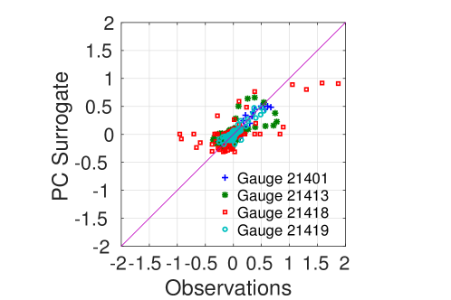
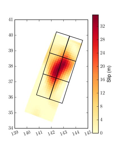
The scatter plot shown in Figure 18 uses inferred MAP values. Thus, the parameters MAP values have reduced the discrepancies between simulated water surface elevation and DART buoy data. This comparison can be seen as an evaluation of the a posteriori goodness-of-fit. Additionally Figure 19 shows the comparison between the MAP values and the Ammon et al. model [30]. Note that the inverted fault leads to a moment and magnitude of $M_{o}=3.43900\times 10^{22}$, $M_{w}=8.99095$, respectively, whereas the Ammon et al. model yields a moment and magnitude of $M_{o}=3.63595\times 10^{22}$ and $M_{w}=9.00708$.

5 Discussion and Conclusions

In this study, we sought to estimate the fault slip distribution that plays a critical role in earthquake and tsunami modeling, mainly in the prediction of water surface elevations. To this end, we proposed a low-dimensional parameterization of the fault slip distribution in which we assumed the fault consists of six sub-faults that have different slip magnitudes. The estimation of the fault slip distribution thus boiled down into a six-parameter inverse problem. A Bayesian inference approach was employed that sharpens the initial estimates of the six uncertain parameters based on measured observations. In our test case, the Tōhoku tsunami, we used water surface elevations information collected at four DART buoy gauges. Discrepancies with measurements were accounted for using a Gaussian noise model, whose variance was treated as a hyper parameter that was inferred along with the uncertain fault parameters.

Bayesian inference was accelerated using a surrogate model constructed based on the Polynomial Chaos approach where the output of the forward model GeoClaw was approximated using PC expansions. The PC expansions were constructed based on a compressed sensing approach that uses basis-pursuit denoising technique, to produce a faithful surrogate. This PC surrogate model was additionally used to quantify the uncertainties in the predicted water surface elevations due to the uncertainties in slip values. This included the mean and standard deviation of water surface elevations.

The present study focused on formulating and estimating a low-dimensional representation of the fault slip distribution using UQ techniques, namely Bayesian inference and PC expansions. A high-dimensional representation of the fault slip distribution would, however, require a large number of forward runs that is computational prohibitive. Instead, one could exploit order-reduction techniques to reduce the dimensionality such as Karhunen-Loève expansions [55]. This will be the objective of a future study.

Figure 1: (Left) The topography, bathymetry and gauge locations used in the simulation, fault is highlighted. (Right) Fault Slip distribution from Ammon et al. [30] with the specified subfault boundaries superimposed.

Figure 2: Parameterized slip values in space. The hypocenter of the earthquake is shown by a marker.

Figure 3: (Left) Observed de-tided water surface height at all the DART buoys used.(Right) Scatter plot of the measured water surface elevation against their GeoClaw model counterparts at the four gauges colored differently. The variance of the difference between the two sets of values is: $7.99\times 10^{-3}~{}m^{2},9.65\times 10^{-3}~{}m^{2},4.62\times 10^{-2}~{}m^{2},5.86\times 10^{-3}~{}m^{2}$ at each gauge.

Figure 4: 2-D projection of the nodes of (Left) Smolyak quadrature and (Right) Latin-Hypercube sample.

Figure 5: 1889 realizations of the evolution of the GeoClaw simulated water surface elevation corresponding to the Smolyak quadrature nodes of PC order 5 at the different gauges.

Figure 6: 729 realizations of the evolution of the GeoClaw simulated water surface elevation corresponding to the LHS sample at the different gauges.

Figure 7: Arrival time function of slip values for the quadrature sample at different gauges.

Figure 8: Maximum Wave Amplitude function of slip values for the quadrature sample at different gauges.

Figure 9: Evolution of NRE between the LHS sample and the corresponding NISP-estimated PC surrogate at the different gauges.

Figure 10: Evolution of NRE between the quadrature sample and the corresponding BPDN-estimated PC surrogate at the different gauges.

Figure 11: Empirical CDF of PC-estimated water surface elevation at the different gauges compared to that of the 1889 runs.

Figure 12: Evolution of the PC-mean water surface elevation at the different gauges.

Figure 13: Chain samples for the six slip values $s_{1},..,s_{6}$. The vertical dotted lines corresponds to the burn-in iterations.

Figure 14: Running mean of the slips values computed using their corresponding MCMC chains.

Figure 15: Chain samples for the four $\sigma^{2}$ the noise variance. The vertical dotted lines corresponds to the burn-in iterations.

Figure 16: KDE of the marginalized posterior distributions for the six slip values $\Pi(s_{1})$ … $\Pi(s_{6})$. The shaded regions corresponds to the 95% intervals of high posterior probability.

Figure 17: KDE of the marginalized posterior distribution of the noise variance $\Pi(\sigma^{2}_{i})$ at each gauge.

Figure 18: Scatter plot of the measured water surface elevation against their PC model counterparts at the four gauges shown in different colors. The PC model was evaluated using the mean of the fault slip posteriors. The variance of the error between the two sets of values is: $2.27\times 10^{-3}~{}m^{2},1.22\times 10^{-2}~{}m^{2},3.32\times 10^{-2}~{}m^{2},2.38\times 10^{-3}~{}m^{2}$ at each gauge.

Figure 19: (Left) MAP of the inferred fault slip values. (Right) Fault slip distribution from Ammon et al.

References

- [1] I. Sraj, K. Mandli, O. M. Knio, I. Hoteit, Uncertainty Quantification and Inference of Manning’s Friction Coefficients using DART Buoy Data during the Tohoku Tsunami, Ocean Modelling 83 (2014) 82–97. doi:10.1016/j.ocemod.2014.09.001.
- [2] B. T. MacInnes, A. R. Gusman, R. J. LeVeque, Y. Tanioka, Comparison of Earthquake Source Models for the 2011 Tohoku Event Using Tsunami Simulations and Near-Field Observations, Bulletin of the Seismological Society of America 103 (2B) (2013) 1256–1274.
-
[3]
A. Sarri, S. Guillas, F. Dias,
Statistical
emulation of a tsunami model for sensitivity analysis and uncertainty
quantification, Natural Hazards and Earth System Science 12 (6) (2012)
2003–2018.
doi:10.5194/nhess-12-2003-2012.
URL http://www.nat-hazards-earth-syst-sci.net/12/2003/2012/ - [4] S. K. Das, R. W. Lardner, Variational parameter estimation for a two‐dimensional numerical tidal model, International Journal for Numerical Methods in Fluids 15 (3) (1992) 313–327.
- [5] R. W. Lardner, Y. Song, Optimal estimation of Eddy viscosity and friction coefficients for a Quasi‐three‐dimensional numerical tidal model, Atmosphere-Ocean 33 (3) (1995) 581–611.
- [6] M. Verlaan, A. W. Heemink, Tidal flow forecasting using reduced rank square root filters, Stochastic Hydrology and Hydraulics 11 (5) (1997) 349–368.
- [7] A. W. Heemink, E. Mouthaan, M. Roest, E. Vollebregt, K. B. Robaczewska, M. Verlaan, Inverse 3D shallow water flow modelling of the continental shelf, Continental Shelf Research 22 (3) (2002) 465–484.
- [8] M. T., T. Butler, C. Dawson, I. Hoteit, Data assimilation within the advanced circulation (adcirc) modeling framework for the estimation of manning’s friction coefficient, Ocean Modelling 76 (2014) 43–58.
- [9] J. Fukuda, K. M. Johnson, A fully bayesian inversion for spatial distribution of fault slip with objective smoothing, Bulletin of the Seismological Society of America 98 (3) (2008) 1128–1146.
- [10] M. Iskandarani, S. Wang, , A. Srinivasan, C. Thacker, J. Winokur, O. Knio, An overview of uncertainty quantification techniques with application to oceanic and oil-spill simulations , Journal of Geophysical Research: Oceans.
- [11] J. Winokur, P. Conrad, I. Sraj, O. Knio, A. Srinivasan, W. C. Thacker, Y. Marzouk, M. Iskandarani, A priori testing of sparse adaptive polynomial chaos expansions using an ocean general circulation model database, Computational Geosciences 17 (6) (2013) 899–911.
- [12] I. Sraj, M. Iskandarani, A. Srinivasan, W. C. Thacker, J. Winokur, A. Alexanderian, C.-Y. Lee, S. S. Chen, O. M. Knio, Bayesian inference of drag parameters using fanapi axbt data, Monthly Weather Review 141 (7) (2013) 2347–2367.
- [13] I. Sraj, M. Iskandarani, A. Srinivasan, W. C. Thacker, O. M. Knio, Drag parameter estimation using gradients and hessian from a polynomial chaos model surrogate, Monthly Weather Review 142 (2) (2014) 933–941.
- [14] P. Mattern, K. Fennel, M. Dowd, Estimating time-dependent parameters for a biological ocean model using an emulator approach, Journal of Marine Systems 96–97 (2012) 32–47. doi:http://dx.doi.org/10.1016/j.jmarsys.2012.01.015.
- [15] M. Reagan, H. Najm, R. Ghanem, O. Knio, Uncertainty quantification in reacting flow simulations through non-intrusive spectral projection, Combustion and Flame 132 (2003) 545–555.
- [16] A. Alexanderian, J. Winokur, I. Sraj, A. Srinivasan, M. Iskandarani, W. Thacker, O. Knio, Global sensitivity analysis in an ocean general circulation model: a sparse spectral projection approach, Computational Geosciences 16 (2012) 757–778, 10.1007/s10596-012-9286-2.
- [17] S. Wang, M. Iskandarani, A. Srinivasan, C. Thacker, J. Winokur, O. Knio, Propagation of uncertainty and sensitivity analysis in an integral oil-gas plume model , submitted.
- [18] I. Sraj, S. Zedler, C. Jackson, O. Knio, I. Hoteit, Polynomial Chaos-based Bayesian Inference of K-Profile Parameterization in a General Circulation Model of the Tropical Pacific, Monthly Weather Review, in review.
- [19] J. Peng, J. Hampton, A. Doostan, A weighted minimization approach for sparse polynomial chaos expansions, Journal of Computational Physics 267 (2014) 92–111.
- [20] G. Li, M. Iskandarani, M. Le Henaff, J. Winokur, O. Le Maitre, O. Knio, Quantifying initial and wind forcing uncertainties in the Gulf of Mexico , Submitted.
- [21] Y. M. Marzouk, H. N. Najm, L. A. Rahn, Stochastic spectral methods for efficient bayesian solution of inverse problems, Journal of Computational Physics 224 (2) (2007) 560–586. doi:{10.1016/j.jcp.2006.10.010}.
- [22] Y. M. Marzouk, H. N. Najm, Dimensionality reduction and polynomial chaos acceleration of bayesian inference in inverse problems, Journal of Computational Phyics 228 (6) (2009) 1862–1902. doi:10.1016/j.jcp.2008.11.024.
[23]
A. Malinverno,
Parsimonious
bayesian markov chain monte carlo inversion in a nonlinear geophysical
problem, Geophysical Journal International 151 (3) (2002) 675–688.
doi:10.1046/j.1365-246X.2002.01847.x.
URL http://dx.doi.org/10.1046/j.1365-246X.2002.01847.x - [24] O. P. Le Maître, O. M. Knio, Spectral Methods for Uncertainty Quantification, Springer-Verlag, 2010.
- [25] F. I. González, R. J. LeVeque, J. Varkovitzky, P. Chamberlain, B. Hirai, D. L. George, GeoClaw results for the NTHMP tsunami benchmark problems, http://depts.washington.edu/clawpack/links/nthmp-benchmarks/ (2011).
- [26] D. L. George, Augmented Riemann solvers for the shallow water equations over variable topography with steady states and inundation, Journal of Computational Physics 227 (6) (2008) 3089–3113.
- [27] M. J. Berger, J. Oliger, Adaptive mesh refinement for hyperbolic partial differential equations, Journal of Computational Physics 52 (1984) 484–512.
- [28] M. J. Berger, R. J. LeVeque, Adaptive Mesh Refinement using Wave-Propagation Algorithms for Hyperbolic Systems, SIAM Journal on Numerical Analysis 35 (1998) 2298–2316.
- [29] C. Amante, B. W. Eakins, ETOPO1 1 Arc-Minute Global Relief Model: Procedures, Data Sources and Analysis, Tech. Rep. NGDC-24, NOAA (Mar. 2009).
- [30] Ammon, A rupture model of the 2011 off the Pacific coast of Tohoku Earthquake, Earth, Planets and Space 63 (7) (2011) 693–696.
- [31] H. B. Milburn, A. I. Nakamura, F. I. González, Real-time tsunami reporting from the deep ocean, in: Oceans 96 MTS/IEEE Conference, Fort Lauderdale, FL, 1996, pp. 390–394.
[32]
G. Mungov, M. Eblé, R. Bouchard,
Dart® tsunameter
retrospective and real-time data: A reflection on 10 years of processing in
support of tsunami research and operations, Pure and Applied Geophysics
170 (9-10) (2013) 1369–1384.
doi:10.1007/s00024-012-0477-5.
URL http://dx.doi.org/10.1007/s00024-012-0477-5 - [33] A. Tarantola, Inverse Problem Theory and Methods for Model Parameter Estimation, SIAM, Philadelphia, PA, 2005.
- [34] D. S. Sivia, Data Analysis - A Bayesian Tutorial, Oxford Science Publications, Oxford, 2006.
[35]
H. Haario, E. Saksman, J. Tamminen,
An adaptive metropolis algorithm,
Bernoulli 7 (2) (2001) 223–242.
URL http://www.jstor.org/stable/3318737 - [36] G. O. Roberts, J. S. Rosenthal, Examples of adaptive MCMC, Journal of Computational and Graphical Statistics 18 (2) (2009) 349–367. arXiv:http://amstat.tandfonline.com/doi/pdf/10.1198/jcgs.2009.06134, doi:10.1198/jcgs.2009.06134.
- [37] D. Xiu, D. Tartakovsky, Uncertainty quantification for flow in highly heterogeneous porous media, in: W. G. G. Cass T. Miller, Matthew W. Farthing, G. F. Pinder (Eds.), Computational Methods in Water Resources: Volume 1, Vol. 55, Part 1 of Developments in Water Science, Elsevier, 2004, pp. 695 – 703.
- [38] R. G. Ghanem, P. D. Spanos, Stochastic Finite Elements: A Spectral Approach, Springer-Verlag, New York, 1991.
- [39] T. Crestaux, O. L. Maitre, J.-M. Martinez, Polynomial chaos expansion for sensitivity analysis, Reliability Engineering & System Safety 94 (7) (2009) 1161 – 1172, special Issue on Sensitivity Analysis.
- [40] M. Berveiller, B. Sudret, M. Lemaire, Stochastic finite element : a non intrusive approach by regression, Eur. J. Comput. Mech. 15 (2006) 81–92.
- [41] P. Constantine, M. Eldred, E. Phipps, Sparse pseudospectral approximation method, Computer Methods in Applied Mechanics and Engineering 229-232 (2012) 1–12.
- [42] P. R. Conrad, Y. Marzouk, Adaptive Smolyak Speudospectral Approximations, SIAM J. Sci. Comp. 35 (6) (2013) 2643–2670.
- [43] G. Blatman, B. Sudret, Adaptive Sparse Polynomial Chaos Expansion Based on Least Angle Regression, J. Comput. Phys. 230 (6) (2011) 2345–2367.
- [44] D. Donoho, Compressed sensing, IEEE Trans. Inform. Theory 52 (2006) 1289–1306.
[45]
E. v. Berg, M. P. Friedlander,
SPGL1: A solver
for large-scale sparse reconstruction (June 2007).
URL http://www.cs.ubc.ca/labs/scl/index.php/Main/Spgl1 -
[46]
E. van den Berg, M. P. Friedlander,
Probing the pareto frontier for
basis pursuit solutions, SIAM Journal on Scientific Computing 31 (2) (2008)
890–912.
doi:10.1137/080714488.
URL http://link.aip.org/link/?SCE/31/890 - [47] K. Petras, On the smolyak cubature error for analytic functions, Advances in Computational Mathematics 12 (2000) 71–93.
- [48] T. Gerstner, M. Griebel, Dimension-adaptive tensor-product quadrature, COMPUTING 71 (1) (2003) 65–87. doi:10.1007/s00607-003-0015-5.
- [49] S. Smolyak, Quadrature and interpolation formulas for tensor products of certain classes of functions, Dokl. Akad. Nauk SSSR 4 (1963) 240–243.
[50]
A. Alexanderian, O. Le Maître, H. Najm, M. Iskandarani, O. Knio,
Multiscale stochastic
preconditioners in non-intrusive spectral projection, Journal of Scientific
Computing (2011) 1–3510.1007/s10915-011-9486-2.
URL http://dx.doi.org/10.1007/s10915-011-9486-2 -
[51]
A. Alexanderian, O. Le Maître, H. Najm, M. Iskandarani, O. M. Knio,
Computing (2011) 1–35doi:10.1007/s10915-011-9486-2.
URL http://dx.doi.org/10.1007/s10915-011-9486-2 - [52] B. Sudret, Global sensitivity analysis using polynomial chaos expansions, Reliability Engineering & System Safety 93 (7) (2008) 964 – 979, bayesian Networks in Dependability. doi:DOI:10.1016/j.ress.2007.04.002.
[53]
E. Parzen, On estimation of a
probability density function and mode, The Annals of Mathematical Statistics
33 (3) (1962) 1065–1076.
URL http://www.jstor.org/stable/2237880 - [54] B. W. Silverman, Density estimation: for statistics and data analysis, Chapman and Hall, London, 1986.
[55]
I. Sraj, O. P. Le Maître, O. M. Knio, I. Hoteit, Coordinate transformation and Polynomial Chaos for the Bayesian inference of a Gaussian process with parametrized prior covariance function, Computer Methods in Applied Mechanics and Engineering 298 (2016) 205–228.doi:10.1016/j.cma.2015.10.002.
URL http://dx.doi.org/10.1016/j.cma.2015.10.002