Cumulants and Correlation Functions vs the QCD phase diagram

Abstract

In this paper we discuss the relation of particle number cumulants and correlation functions. It is argued that measuring couplings of the genuine multi-particle correlation functions could provide cleaner information on possible non-trivial dynamics in heavy-ion collisions. We extract integrated multi-proton correlation functions from the presently available experimental data on proton cumulants. We find that the STAR data contain significant four-proton correlations, at least at the lower energies, with indication of changing dynamics in central collisions. We also find that these correlations are rather long-ranged in rapidity. Finally, using the Ising model, we demonstrate how the signs of the multi-proton correlation functions may be used to exclude certain regions of the phase diagram close to the critical point.

I Introduction

The search for structures in the QCD phase diagram, such as a critical point or a first order phase coexistence region has been at the forefront of strong interaction research for the last several years. Most experimental and theoretical effort in this regard has concentrated on the measurement and calculation of cumulants of conserved charges, in particular of baryon number cumulants Stephanov et al. (1998); Stephanov (2009); Skokov et al. (2011); Friman et al. (2011); Kitazawa et al. (2014); Adamczyk et al. (2014a, b), see, e.g., Koch (2010) for an overview. Different ideas, based on an intermittency analysis in the transverse momentum phase space are also explored Anticic et al. (2010, 2015).

Cumulants of the particle number distribution have the advantage that they are easily accessible in finite temperature field theory since they are simply given by derivatives of the free energy with respect to an appropriate chemical potential. However they have the disadvantage that they mix correlations of different order. For example in case of a system of uncorrelated particles of one species, say protons, governed by the Poisson distribution, all cumulants are given by the mean number of particles, $K_{i}=\langle N\rangle$ for all $i$. Similarly, for system of uncorrelated resonances which decay in two particles, the cumulants are simply given by $K_{i}=2^{i}\langle N_{\text{res}}\rangle$, with $\langle N_{\text{res}}\rangle$ the average number of resonances. Therefore, a large value for the forth order cumulant does not necessarily mean the presence of strong four-particle correlations (in our illustrative case we have only two-particle correlations). Consequently, the fact that STAR sees a cumulant ratio for protons of $K_{4}/K_{2}\simeq 3.5$ at $\sqrt{s}=7.7{\rm\,GeV}$ Luo (2015) may well be the result of strong two particle correlations, rather than three and four body correlations, which would be expected close to a critical point Stephanov (2009).

Therefore, it would be very valuable if the true correlation functions could be extracted from the measured cumulants. In this paper we will discuss how this can be done, at least for the case of one species of particles, such as protons (see also Ling and Stephanov (2016)). For net-proton cumulants, i.e. cumulants of the difference distribution of protons and anti-protons, this is unfortunately not the case. However, at the beam energies where STAR sees the strongest deviation from Poisson behavior, the number of anti-proton to proton ratio is vanishingly small and thus the anti-protons can be ignored.

This paper is organized as follows. First we demonstrate how the true correlation functions can be related to the cumulants, then we apply these relations to the preliminary STAR data. Next we discuss the centrality, rapidity, and energy dependence of these correlation functions. Finally we illustrate how just the information about the signs of these correlation functions can be used to exclude certain regions around the critical point.

II Cumulants and Correlations Functions

Let us start by introducing the correlation functions, beginning with two particles. The two particle density for particles with momenta $p_{1}$ and $p_{2}$, $\rho_{2}\left(p_{1},p_{2}\right)$, is given by

$$\rho_{2}(p_{1},p_{2})=\rho_{1}(p_{1})\rho_{1}(p_{2})+C_{2}(p_{1},p_{2}),$$ (1)

where $\rho_{1}\left(p\right)$ refers to the one particle density, and $C_{2}(p_{1},p_{2})$ represents the two-particle correlation function.

In general the two particle density and correlation function depend on the momenta of both particles. In the following, we will restrict ourselves to correlations in rapidity and adopt the following notation

$$\rho_{2}\left(y_{1},y_{2}\right) = \int dp_{t,1}d\phi_{1}dp_{t,2}d\phi_{2}\rho_{2}\left(p_{1},p_{2}\right),$$

$$C_{2}\left(y_{1},y_{2}\right) = \int dp_{t,1}d\phi_{1}dp_{t,2}d\phi_{2}C_{2}\left(p_{1},p_{2}\right),$$

$$C_{2} = \int dy_{1}dy_{2}C_{2}\left(y_{1},y_{2}\right),$$ (2)

and similarly for higher order particle densities and correlation functions.

Integrating $\rho_{2}(p_{1},p_{2})$ over the momenta we obtain

$$F_{2}\equiv\left\langle N\left(N-1\right)\right\rangle=\int dp_{1}dp_{2}\,\rho_{2}(p_{1},p_{2})=\left\langle N\right\rangle^{2}+C_{2},$$ (3)

where $N$ is the number of particles under consideration and $C_{2}$ is the integrated two-particle correlation function. In the absence of correlations, $C_{2}(p_{1},p_{2})=0$, we obtain $\langle N^{2}\rangle-\langle N\rangle^{2}=\langle N\rangle$.

The three particle density depends on the single-particle densities as well as the two and three-particle correlation functions

$$\rho_{3}(y_{1},y_{2},y_{3}) = \rho_{1}(y_{1})\rho_{1}(y_{2})\rho_{1}(y_{3})+\rho_{1}(y_{1})C_{2}(y_{2},y_{3})+\rho_{1}(y_{2})C_{2}(y_{1},y_{3})$$ (4)

$$+\,\rho_{1}(y_{3})C_{2}(y_{1},y_{2})+C_{3}(y_{1},y_{2},y_{3}),$$

and is related to the third order factorial moment $F_{3}=\left\langle N\left(N-1\right)\left(N-2\right)\right\rangle$ via

$$F_{3}=\int dy_{1}dy_{2}dy_{3}\rho_{3}\left(y_{1},y_{2},y_{3}\right)=F_{1}^{3}+3F_{1}C_{2}+C_{3},$$ (5)

where $C_{3}$ is the integrated genuine three-particle correlation function and $F_{1}=\langle N\rangle$. Similarly the higher order factorial moments are given by

$$F_{4} = F_{1}^{4}+6F_{1}^{2}C_{2}+4F_{1}C_{3}+3C_{2}^{2}+C_{4},$$ (6)

$$F_{5} = F_{1}^{5}+5F_{1}C_{4}+10F_{1}^{2}C_{3}+10F_{1}^{3}C_{2}+15F_{1}C_{2}^{2}+10C_{2}C_{3}+C_{5},$$ (7)

$$F_{6} = F_{1}^{6}+6F_{1}C_{5}+15F_{1}^{2}C_{4}+20F_{1}^{3}C_{3}+15F_{1}^{4}C_{2}+60F_{1}C_{2}C_{3}+45F_{1}^{2}C_{2}^{2}+15C_{2}C_{4}+10C_{3}^{2}+15C_{2}^{3}+C_{6}.$$ (8)

Before we discuss the connection between the integrated correlation functions and the cumulants, for completeness let us discuss a more formal way of calculating multi-particle integrated correlation functions. The above formulas connect the factorial moments $F_{i}$ with the integrated correlation functions $C_{n}$. For example, $C_{2}=F_{2}-F_{1}^{2}$ (see Eq. (3)), which is simply $\langle N(N-1)\rangle-\langle N\rangle^{2}$. In other words, the integrated correlation functions can be expressed in terms of the factorial moments of the multiplicity distribution. Suppose that the particles under consideration are characterized by the multiplicity distribution $P(N)$, where $N$ in our case is the number of protons. The factorial moment $F_{k}=\langle N!/(N-k)!\rangle$ is conveniently calculated using the generating function $H(z)$

$$F_{k}=\left.\frac{d^{k}}{dz^{k}}H(z)\right|_{z=1},\qquad H(z)=\sum\nolimits_{N}P(N)z^{N},\qquad H(1)=1,$$ (9)

and the integrated correlation function is given by analogous derivatives from the logarithm of $H(z)$.

$$C_{n}=\left.\frac{d^{n}}{dz^{n}}\ln\left[H(z)\right]\right|_{z=1}.$$ (10)

For example, $C_{2}=H^{{}^{\prime\prime}}(1)-(H^{{}^{\prime}}(1))^{2}=F_{2}-F_{1}^{2}$, in agreement with Eq. (3), and it is straightforward to verify Eqs. (5-8) as well.

The particle number cumulants, $K_{n}$, can be expressed in terms of the factorial moments Bzdak and Koch (2012),

$$K_{1} \equiv \langle N\rangle=F_{1},$$

$$K_{2} \equiv \langle(\delta N)^{2}\rangle=F_{1}-F_{1}^{2}+F_{2},$$

$$K_{3} \equiv \langle\left(\delta N\right)^{3}\rangle=F_{1}+2F_{1}^{3}+3F_{2}+F_{3}-3F_{1}(F_{1}+F_{2}),$$ (11)

and

$$K_{4} \equiv \langle\left(\delta N\right)^{4}\rangle-3\langle(\delta N)^{2}\rangle^{2}$$ (12)

$$= F_{1}-6F_{1}^{4}+7F_{2}+6F_{3}+F_{4}+12F_{1}^{2}(F_{1}+F_{2})-3(F_{1}+F_{2})^{2}-4F_{1}(F_{1}+3F_{2}+F_{3}),$$

where $\delta N=N-\langle N\rangle$. Formulas for the higher order cumulants can be found in Ref. Bzdak and Koch (2012).

We note that in the present paper we are interested in the multi-proton correlation functions and thus we consider cumulants and correlations for protons only. In the above equations $N$ denotes the number of protons and not the net-proton number.

Now we can relate the cumulants in terms of the correlation functions and the mean particle number $\langle N\rangle=F_{1}$

$$K_{2} = \left\langle N\right\rangle+C_{2},$$ (13)

$$K_{3} = \left\langle N\right\rangle+3C_{2}+C_{3},$$ (14)

$$K_{4} = \left\langle N\right\rangle+7C_{2}+6C_{3}+C_{4},$$ (15)

and vice versa

$$C_{2} = -\left\langle N\right\rangle+K_{2},$$ (16)

$$C_{3} = 2\left\langle N\right\rangle-3K_{2}+K_{3},$$ (17)

$$C_{4} = -6\left\langle N\right\rangle+11K_{2}-6K_{3}+K_{4}.$$ (18)

Before we apply the above equations to extract the correlation strength from the STAR data, let us make a few more remarks concerning these correlation functions.

It should be clear from Eqs. (16)-(18) that as we approach the critical point, $C_{n}$ is dominated by $K_{n}$ which scales with the highest power of the correlation length $\xi$ Stephanov (2009). Thus, following Stephanov (2009), $C_{2}\sim\xi^{2}$, $C_{3}\sim\xi^{4.5}$, and $C_{4}\sim\xi^{7}$ close to the critical point.

Frequently in the literature, see, e.g., Ref. Lisa et al. (2005), one refers to correlation function where the trivial dependence on the particle density/multiplicity is removed

$$c_{n}\left(y_{1},...,y_{n}\right)=\frac{C_{n}\left(y_{1},...,y_{n}\right)}{\rho_{1}\left(y_{1}\right)\cdots\rho_{1}\left(y_{n}\right)},$$ (19)

which we shall refer to as reduced correlation functions or simply couplings. For example in terms of the reduced correlation functions the two particle density would be given as

$$\rho_{2}\left(y_{1},y_{2}\right)=\rho_{1}\left(y_{1}\right)\rho_{1}\left(y_{2}\right)\left[1+c_{2}\left(y_{1},y_{2}\right)\right].$$ (20)

The reduced correlation functions will prove helpful when studying for instance the centrality dependence of the correlations. Integrating Eq. (19) over rapidity we obtain

$$C_{k}=\left\langle N\right\rangle^{k}c_{k},$$ (21)

where $\left\langle N\right\rangle=\int_{\Delta y}\rho_{1}(y)dy$ depends on the rapidity interval $\Delta y$ and we denote

$$c_{k}=\frac{\int\rho_{1}\left(y_{1}\right)\cdots\rho_{1}\left(y_{k}\right)c_{k}\left(y_{1},...,y_{k}\right)dy_{1}\cdots dy_{k}}{\int\rho_{1}\left(y_{1}\right)\cdots\rho_{1}\left(y_{k}\right)dy_{1}\cdots dy_{k}}.$$ (22)

Using above definition we can write

$$K_{2} = \left\langle N\right\rangle+\left\langle N\right\rangle^{2}c_{2},$$ (23)

$$K_{3} = \left\langle N\right\rangle+3\left\langle N\right\rangle^{2}c_{2}+\left\langle N\right\rangle^{3}c_{3},$$ (24)

$$K_{4} = \left\langle N\right\rangle+7\left\langle N\right\rangle^{2}c_{2}+6\left\langle N\right\rangle^{3}c_{3}+\left\langle N\right\rangle^{4}c_{4}.$$ (25)

Finally we should point out that a direct relation between correlation functions and cumulants can not be established if one considers for example net-proton cumulants. In this case the additional knowledge of various factorial moments is required. The relevant formulas are given in the Appendix.

II.1 Comments

Before we analyze the existing data several comments are warranted.

• First it would be interesting to see how the correlation functions $C_{n}$ and couplings $c_{n}$ scale with multiplicity if the correlations originate from independent sources of correlations, e.g., from resonances/clusters or when A+A is a simple superposition of elementary p+p interactions. This will be useful when studying the centrality dependence of the correlations.

  Suppose we have $N_{s}$ sources of particles, each characterized by the multiplicity distribution $P(n_{i})$. The final multiplicity distribution is given by

  $$P(N)=\sum_{n_{1},n_{2},...,n_{N_{s}}}P(n_{1})P(n_{2})\cdots P(n_{N_{s}})\delta_{n_{1}+...+n_{N_{s}}-N}.$$ (26)

  Calculating the factorial moment generating function we obtain

  $$H(z)=\sum\nolimits_{N}P(N)z^{N}=\left(\sum\nolimits_{n_{1}}P(n_{1})z^{n_{1}}\right)^{N_{s}}=H_{1}(z)^{N_{s}},$$ (27)

  where $H_{1}(z)$ is the factorial moment generating function from a single source. The correlation function, $C_{k}$, is given by

  $$C_{k}=\left.\frac{d^{k}}{dz^{k}}\ln\left[H(z)\right]\right|_{z=1}=N_{\text{s}}\left.\frac{d^{k}}{dz^{k}}\ln\left[H_{1}(z)\right]\right|_{z=1}=N_{s}C_{k}^{(\text{source})},$$ (28)

  where $C_{k}^{(\text{source})}$ is the correlation from a single source. As seen from the above equation $C_{k}$ scales simply with the number of sources since $C_{k}^{(\text{source})}$, being a property of a single independent source, does not depend on $N_{s}$. Comparing Eq. (28) with Eq. (21) we obtain

  $$c_{k}=\frac{N_{s}}{\left\langle N\right\rangle^{k}}C_{k}^{(\text{source})},$$ (29)

  and assuming that the number of produced protons, $N$, is proportional to the number of sources we have for the couplings

  $$c_{k}\sim\frac{1}{\left\langle N\right\rangle^{k-1}}.$$ (30)

  This result is rather straightforward. The correlation strength, $c_{k}$, for the whole system gets diluted once there are many independent sources of correlations. Suppose we have $N_{s}$ sources which correlate two particles each. Then we have $N=2N_{s}$ particles and $N_{s}=N/2$ correlated pairs. The total number of pairs is $N(N-1)/2\simeq 2N_{s}^{2}$ and thus the number of correlated over all pairs scales like $1/N$. Similarly for triplets (now each source correlates three particles) one gets $N/3$ correlated out of $N(N-1)(N-2)/3!\simeq N^{3}/3!$ total triplets, leading to $1/N^{2}$. The scaling, Eq. (30), is expected, e.g., for resonances / clusters of particles or when A+A can be decomposed into elementary p+p collisions.

  We note that the scaling given by Eq. (30) is expected to break down when the sources are not independent. For example when we have one coherent source of correlations, the number of correlated pairs might be proportional to the total number of pairs and $c_{k}$ could become constant

  $$c_{k}\sim\text{const}.$$ (31)

  as a function of $N$. It would be definitely interesting to observe such transition (from $1/N^{k-1}$ to const.) in experimental data. In the next section we will argue that this is the case for central collisions in the preliminary STAR data at the lowest energies.

• Suppose that indeed $c_{2,3,4}$ are constant or depend only very weakly on the number of produced protons. In this case the correlations, $C_{k}=\langle N\rangle^{k}c_{k}$, increase with the number of particles. One scenario would be that the sources of correlation are correlated themselves or that the sources correlate increasing number of particles, e.g., with increasing $N$ clusters get larger (more particles per cluster) leading to $C_{k}^{(\text{source})}$ depending on $N$, see Eq. (29). Given only the integrated reduced correlation function, it is impossible to distinguish between these various scenarios. In any case, centrality independence of the couplings, indicate that the increasing number of particles are correlated and, for the lack of a better term, we will refer to this behavior as “collective”. In this case the cumulants, $K_{n}$, explicitly depend on $\langle N\rangle^{i}$, $i=1,2,...,n$, see Eqs. (23-25). Consequently the cumulant ratios depend on multiplicity which makes the interpretation of the data rather complicated. For example by changing centrality or energy we obviously change $\langle N\rangle$ which may result in nontrivial behavior. For example if $\langle N\rangle\ll 1$, as in the case of anti-protons at low energy, the cumulants are dominated by the leading term and the cumulant ratios are close to $1$ even if couplings carry actually some nontrivial information.

  We conclude that the cumulant ratios are rather tricky to interpret if the couplings, $c_{k}$, are constant as a function of produced protons. It seems that studying correlation functions is more appropriate in this case.

• Similarly we can make some general observations about the rapidity dependence of cumulants and their ratios. To this end let us consider two limits and let us assume the rapidity density is constant, $dN/dy=\rho_{1}(y)=\text{const}$ in rapidity window of interest:

  (a) The correlations are local in rapidity and depend only on the relative distances, $c_{k}(y_{1},\ldots,y_{k})=c_{k}^{0}\delta(y_{1}-y_{2})\cdots\delta(y_{k-1}-y_{k})$. In this case the couplings or reduced correlation functions, Eq. (22), are given by $c_{n}=c_{n}^{0}/(\Delta y)^{n-1}$, where $\Delta y$ is the range in rapidity under consideration (namely, particles are measured in $-\Delta y/2<y<\Delta y/2$). Consequently, the correlation functions $C_{n}$ and the cumulants scale linearly with $\Delta y$

  $$C_{n}\sim\Delta y\quad\rightarrow\quad K_{n}\sim\Delta y.$$ (32)

  In this case the cumulant ratios, e.g., $K_{4}/K_{2}$, do not depend on $\Delta y$.

  (b) The other extreme are long-range correlations, where the correlation functions are constant over the rapidity region of interest. In this case $c_{k}(y_{1},\ldots,y_{k})=c_{k}^{0}$ and $c_{k}$, defined in Eq. (22), equals $c_{k}^{0}$. Thus the correlation functions, $C_{n}=\langle N\rangle^{n}c_{n}$, scale with the n-th power of the rapidity interval $\Delta y$

  $$C_{n}\sim(\Delta y)^{n},$$ (33)

  since $\langle N\rangle\sim\Delta y$. The scaling of the cumulants $K_{n}$ in this case is more subtle since the cumulants depend on correlation functions of various order. For example the fourth order cumulant

  $$K_{4}=\left\langle N\right\rangle+7\left\langle N\right\rangle^{2}c_{2}^{0}+6\left\langle N\right\rangle^{3}c_{3}^{0}+\left\langle N\right\rangle^{4}c_{4}^{0},\qquad\left\langle N\right\rangle=\left\langle N_{\Delta y=1}\right\rangle\Delta y,$$ (34)

  depends on the correlation functions $C_{2}$ to $C_{4}$ and the dependence of $\Delta y$ is thus a polynomial of up to fourth order in $\Delta y$. Here $\langle N_{\Delta y=1}\rangle$ is the average number of particles in $\Delta y=1$. In this case the cumulant ratios do depend (in general) on the size of the rapidity window $\Delta y$. We will discuss this issue in more detail in the next section.

  Of course things get more complicated if the rapidity density $dN/dy$ is not constant and if the correlation length in rapidity is finite but shorter than $\Delta y$.

• It is clear that at very low energy the majority of observed protons originate from the incoming nuclei, and are decelerated to mid rapidity. In the simplest model we may assume that protons stop in a given rapidity $\Delta y$ bin with some probability $p$ leading to binomial distribution

  $$P(N)=\frac{B!}{N!(B-N)!}p^{N}(1-p)^{B-N},$$ (35)

  where $B$ is the total number of protons (that potentially can stop in $\Delta y$) and $pB$ is the mean number of protons observed in a given acceptance. We note that the above formula, representing the simplest stopping model, is equivalent to the problem of global baryon conservation Bzdak et al. (2013), when the contribution from anti-protons may be neglected (low energies). The factorial moment generating function is

  $$H(z)=\sum\nolimits_{N}P(N)z^{N}=\left[1-p(1-z)\right]^{B},$$ (36)

  and the couplings are

  $$c_{2}=-\frac{1}{B},\quad c_{3}=\frac{2}{B^{2}},\quad c_{4}=-\frac{6}{B^{3}}.$$ (37)

  We note that $B$ is changing with centrality and this scenario falls into the class of independent sources of correlations, since protons stop independently in $\Delta y$.

• It would be interesting to measure correlations and couplings between protons and anti-protons and how they change with energy and centrality. In the Appendix we derive suitable formulas, which require the knowledge of additional factorial moments.

• The preliminary STAR data Luo (2015) show a comparatively large ratio of the fourth-order over second-order cumulant, $K_{4}/K_{2}\simeq 3.5$. Given Eqs. (13) and (15) this does not imply a priori the presence of any four particle correlations, since for sufficiently large two-particle correlations, $C_{2}\gg\left\langle N\right\rangle$, the cumulant ratio may be as large as $K_{4}/K_{2}\simeq 7$ without any three- and four-particle correlations.

III Extracting correlation functions from data

Figure 1: Centrality dependence of the two- three- and four-proton correlation functions $C_{2},C_{3},C_{4}$ for collision energies $\sqrt{s}=7.7{\rm\,GeV}$ (a), $11.5{\rm\,GeV}$ (b), and $19.6{\rm\,GeV}$ (c). Results are based on preliminary STAR data Luo (2015).

Having defined the correlation functions and their relation to the cumulants we can now proceed to extract them from the measured proton number cumulants obtained by the STAR collaboration Adamczyk et al. (2014a); Xu (2014); Luo (2015). Here we will concentrate on the preliminary data which cover the transverse momentum range $0.4{\rm\,GeV}<p_{t}<2.0{\rm\,GeV}$ Luo (2015).

Our goal is to extract information about correlations between protons, given by the genuine multi-proton integrated correlation functions, $C_{n}$ and $c_{n}$, using the measured cumulants for protons (not net-proton). It would be also interesting to extract analogous information about the antiproton correlation functions (or even proton-antiproton correlations, see Appendix), however, in this paper we are interested in the lowest beam energies, where the number of antiprotons is small. Let us add here that the cumulant ratio, $K_{4}/K_{2}$, is very similar for protons and net-protons for all measured energies, see a recent review Luo and Xu (2017), including $7.7$ GeV where $K_{4}/K_{2}$ is particularly large.

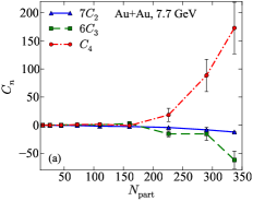
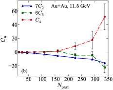
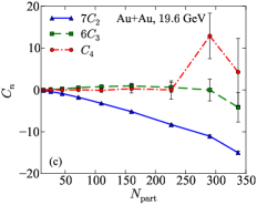
Let us start with the correlation functions $C_{n}$, Eqs. (16-18). They are shown in Fig. 1 as a function of centrality for the three energies, $\sqrt{s}=7.7{\rm\,GeV},\,11.5{\rm\,GeV}\,{\rm and}\,19.6{\rm\,GeV}$. Note that we have multiplied the correlation functions with the appropriate factors so that they reflect their contribution to the fourth order cumulant, Eq. (15). For the two most central points, we find that for all three energies the four-proton correlations are finite and positive, $C_{4}>0$, whereas the two- and three-proton correlations are negative, $C_{2},C_{3}<0$. In addition, for $\sqrt{s}=7.7{\rm\,GeV}$ $C_{4}$ is clearly the dominant contribution to the fourth order cumulant. Thus, the steep rise in the $K_{4}/K_{2}$ cumulant ratio seen in the preliminary STAR data Luo (2015) is indeed due to four-proton correlations. For $\sqrt{s}=19.6{\rm\,GeV}$ on the other hand we find that for the most central point the negative two-particle correlation is the dominant contribution to the fourth order cumulant. Therefore, the fact that the preliminary STAR data show a cumulant ratio below the Poisson baseline, $K_{4}/K_{2}<1$, is due to negative two-proton rather than negative four-proton correlations.

Figure 2: Centrality dependence of three-proton reduced correlation functions $c_{3}$ for collision energies $\sqrt{s}=7.7{\rm\,GeV}$ (a), $11.5{\rm\,GeV}$ (b), and $19.6{\rm\,GeV}$ (c). The horizontal long-dashed line separates positive from negative values. The short dashed lines represent an expectation from the independent source model, $c_{3}\sim 1/\left\langle N\right\rangle^{2}$ with $\left\langle N\right\rangle$ being the number of measured protons. The full lines adds a constant offset to the independent source model. Results are based on preliminary STAR data Luo (2015).

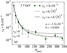
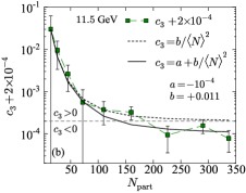
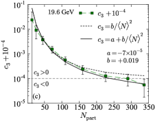
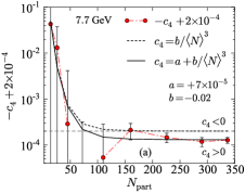
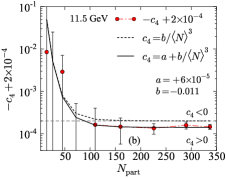
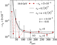
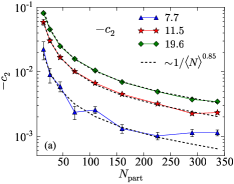
Next we turn to the reduced correlation functions, $c_{2},c_{3},c_{4}$, Eq. (22). In Figs. 2, 3 and  4 (panel (a)) we show their centrality dependence for the three energies under consideration. We find that the reduced two-proton correlations or couplings, $c_{2}$, for all energies scale like $1/\left\langle N\right\rangle^{0.85}$, with $\left\langle N\right\rangle$ being the number of protons, which is close to the $1/\left\langle N\right\rangle$ scaling expected from independent sources, but sufficiently different that this behavior deserves further investigation. At present we have no obvious explanation for this deviation from independent source scaling.

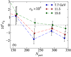
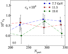
For $N_{\rm part}<200$ the three- and four-proton couplings, within errors, are consistent with $1/\left\langle N\right\rangle^{2}$ and $1/\left\langle N\right\rangle^{3}$ scaling, respectively. In addition the three- and four-proton couplings change sign around $N_{\rm part}\simeq 200$ whereas $c_{2}$ remains negative for all centralities. At roughly the same centrality, the three- and four-proton couplings flatten out, most prominently at the lowest two energies. Concentrating on the lowest energy, $\sqrt{s}=7.7{\rm\,GeV}$, we find that for $N_{\rm part}>200$ all three reduced correlation functions remain constant, indicating stronger correlations than an independent source picture would suggest. As discussed above, this “collective” behavior may be due to either correlations among the sources or due to sources which correlate increasingly more particles (e.g., clusters increase their particle content with increasing $N$). It is interesting to note, that the transition from independent source scaling to “collective” behavior is accompanied with a change of sign of the three- and four-proton couplings. Apparently some new dynamics comes into play at $N_{\rm part}\simeq 200$. The two right panels of Fig. 4 show this region in more detail. It appears that the centrality independence is most significant for the lower energies, whereas it would be difficult to argue for a centrality independence, especially for $c_{3}$, at $19.6{\rm\,GeV}$.

We note that the purpose of the solid and dashed lines presented in Figs. 2, 3 and  4 (panel (a)) is to guide the eye and demonstrate that the preliminary STAR data are roughly consistent (except most central collisions) with $c_{k}\sim 1/\left\langle N\right\rangle^{k-1}$ expected from the independent source model, where $\left\langle N\right\rangle$ is the number of protons at a given centrality. Finally, let us also add that according to the preliminary STAR data $\left\langle N\right\rangle\sim N_{\rm part}^{1.25}$, which allows to translate the number of protons to the number of participants.

Figure 3: Same as Fig. 2 but for the four-proton reduced correlation function $c_{4}$.

Figure 4: Panel (a): Centrality dependence of two-proton reduced correlation functions $c_{2}$ for collision energies $\sqrt{s}=7.7{\rm\,GeV}$, $11.5{\rm\,GeV}$, and $19.6{\rm\,GeV}$. The dashed lines are to guide the eye and demonstrate that $c_{2}\sim 1/\left\langle N\right\rangle^{0.85}$, where $\left\langle N\right\rangle$ is the number of protons. Panel (b): Most central points for the three-proton reduced correlation $c_{3}$ function for energies $\sqrt{s}=7.7{\rm\,GeV}$, $11.5{\rm\,GeV}$, and $19.6{\rm\,GeV}$. Panel (c): Most central points for the four-proton reduced correlation function $c_{4}$ for energies $\sqrt{s}=7.7{\rm\,GeV}$, $11.5{\rm\,GeV}$, and $19.6{\rm\,GeV}$. Results are based on preliminary STAR data Luo (2015).

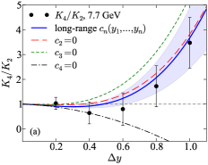
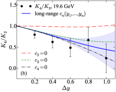
Next let us turn to the dependence of the cumulant ratio $K_{4}/K_{2}$ on the size of the rapidity window $\Delta y$, where protons are accepted. Preliminary results of this ratio has been shown by STAR for rapidity windows up to $\Delta y\leq 1$ Luo (2015). As discussed in section II.1 the cumulant ratio $K_{4}/K_{2}$ is constant in case of short range correlations in rapidity. For long range correlations, on the other hand, the dependence of the cumulants on the rapidity is a given by a polynomial of up to $n^{\rm{th}}$ order, where $n$ is the order of the cumulant. In Fig. 5 we show the preliminary STAR data Luo (2015) for both $7.7{\rm\,GeV}$ and $19.6{\rm\,GeV}$ together with the results assuming long range correlations. Clearly the STAR data show a significant dependence on $\Delta y$, ruling out short-range correlations. The predictions based on long-range correlations, on the other hand, agree with the preliminary STAR data rather well.

The blue solid lines in Fig. 5 were generated using Eq. (34) for $K_{4}$ and an analogous expression for $K_{2}$. From the preliminary STAR data we have $\langle N_{\Delta y=1}\rangle=39.3$ for central $7.7$ GeV and $24.9$ for $19.6$ GeV. Using $\langle N\rangle=\langle N_{\Delta y=1}\rangle\Delta y$ we obtain the rapidity dependence of $\langle N\rangle$. In case of long-range correlation there are three unknown parameters $c_{n}^{0}$ for $n=2,3,4$. We determine them using the STAR values of $K_{2,3,4}$ at $\Delta y=1$, which allow to calculate $C_{n}$ and consequently $c_{n}=c_{n}^{0}$. Having $c_{n}^{0}$ (determined from $\Delta y=1$) we can calculate $K_{4}/K_{2}$ for arbitrary values of $\Delta y$.

In Fig. 5 we also show the resulting rapidity dependence when we set one of the couplings to zero. For $7.7{\rm\,GeV}$ setting $c_{2}=0$ makes hardly any difference and even $c_{3}=0$ bring the result close within errors. Clearly, as already emphasized, the ratio $K_{4}/K_{2}$ for central $7.7{\rm\,GeV}$ collisions is dominated by four-proton correlations. This is different for $19.6{\rm\,GeV}$ shown in panel (b). The $K_{4}/K_{2}$ ratio drops more or less linearly with $\Delta y$. This dependence suggests that the second order correlation function $C_{2}$ dominates the cumulant ratio, and that $C_{2}$ is negative. This is quantified by our results. While $c_{3}=0$ or $c_{4}=0$ still gives reasonable agreement, setting $c_{2}=0$ totally misses the data. This observation supports our previous finding that the drop in the cumulant ratio below the Poisson limit, $K_{4}/K_{2}<1$ at $19.6{\rm\,GeV}$ originates from negative two-proton correlation.

Figure 5: Dependence on the rapidity window $\Delta y$ of the cumulant ratio $K_{4}/K_{2}$. The full line corresponds to our prediction assuming long-range correlations (see text fore details). The shaded area represent the error on this prediction. The long-dashed (red), short-dashed (green) and dot-dashed (black) curve correspond to setting $c_{2}=0$ or $c_{3}=0$ or $c_{4}=0$, respectively. Panel (a) is for $\sqrt{s}=7.7{\rm\,GeV}$ and panel (b) for $\sqrt{s}=19.6{\rm\,GeV}$. The data are preliminary STAR results Luo (2015).

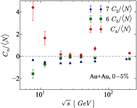
Finally in Fig. 6 we show the energy dependence of the cumulants $C_{n}$ which we scaled by the number of particles, $C_{n}/\left\langle N\right\rangle$ and multiplied by the appropriate factors to reflect their relative contribution to the fourth order cumulant, Eq. (15). Here we include points for the proton correlations up to $\sqrt{s}=200{\rm\,GeV}$ to show the overall trend although at energies larger that $19.6{\rm\,GeV}$ anti-protons become non-negligible, and thus the physical interpretation is less clear. In spite of that there seems to be a clear trend as we lower the energy. Aside from an excursion at $62.4{\rm\,GeV}$ the scaled four-particle correlation seems to be small, slightly positive before it significantly increases for the two lowest energies. Clearly the excursion at $62.4{\rm\,GeV}$ needs further scrutiny. Similarly, the scaled three-proton correlation stays flat and negative before it decreases even further at the lowest energy. The scaled two-particle correlation, on the other hand, seem to exhibit a shallow minimum around $20-30{\rm\,GeV}$. At lower energies it tends towards zero, and one might be inclined to speculate that it may turn positive at even lower energies. Needless to say, the strong energy dependence of the three- and four-proton correlations together with the prospect of the two particle correlation changing sign warrants measurements at even lower energies.

Figure 6: Energy dependence for the scaled correlation functions $C_{n}/\left\langle N\right\rangle$ weighted with the appropriate factor to reflect the relative contribution to the fourth order cumulant $K_{4}$ (see Eq. (15)). The 200 GeV point for $C_{2}$ is shifted for clarity. Results are based on preliminary STAR data Luo (2015).

To summarize this section, we have used the preliminary STAR data on proton cumulants to extract information about the correlation functions and couplings for protons. We find that at the lowest beam energy of $7.7{\rm\,GeV}$ there are significant four-proton correlations which dominate the fourth order cumulant. At $19.9{\rm\,GeV}$, on the other hand, the fourth order cumulant is dominated by a negative two-proton correlation. We further observed that for the lowest energies the centrality dependence change from that of an independent source model to a “collective” one at $N_{\rm part}\simeq 200$. At about the same centrality the three- and four-proton couplings change sign, indicating a change in the underlying dynamics. Finally, an analysis of the rapidity dependence indicates that the correlations are long-range in rapidity. Of course given the fact that $\Delta y\leq 1$ we can not rule out a finite correlation length which is somewhat larger that $\delta y=1$. The rapidity dependence also confirms our finding that the cumulant ratio $K_{4}/K_{2}$ is dominated by (positive) four-proton correlations at $7.7{\rm\,GeV}$ and by (negative) two-proton correlations at $19.6{\rm\,GeV}$. Finally, the scaled correlations show interesting dependence on the energy especially at the lowest available energies, which clearly calls for measurements at even lower energies that $\sqrt{s}=7.7{\rm\,GeV}$.

IV Potential implications for the search of a critical point

In this section we want to explore to which extent the signs of the correlation functions $C_{2},C_{3},C_{4}$ can be used to exclude regions around a QCD critical point. Here we use universality arguments in analogy to Nonaka and Asakawa (2005); Stephanov (2011) exploiting the fact that the critical point belongs to the Ising universality class. This exercise should be considered a feasibility study with the aim to demonstrate that the signs of the correlation functions provide already very important information. For a more quantitative analysis of experimental data, additional effects need to be accounted for Hippert et al. (2016). For example it is known that the non-equilibrium effects can significantly alter the cumulants and the correlation functions Kitazawa et al. (2014); Mukherjee et al. (2015); Herold et al. (2016). These effects and possibly others, need to be corrected for in an analysis of experimental data before any comparison with an equilibrium phase diagram is possible. We emphasize again that our goal here is simply to demonstrate that the signs of the correlation functions carry non-trivial information and, when all effects are taken into account (if at all possible), could be used to exclude certain regions of the QCD phase-diagram.

In the scaling domain density and reduced temperature in the QCD setting can be mapped to the Ising variables reduced temperature $t$ and magnetic field $H$. The precise mapping to the conventionally used coordinates temperature $T$ and chemical potential $\mu$ is of no relevance for this argument, we only note that $H=t=0$ maps to the critical point and that the reduced temperature axis $t$ is tangential to the phase boundary at the critical point. The simplest qualitative parametrizations of freeze-out lines in terms of Ising variables is given by $H=\text{const.}$ lines, see also the discussion in Nonaka and Asakawa (2005); Stephanov (2011). Furthermore, the signs of correlation functions do not really depend on the variables used, we avoid a discussion of the precise mapping from Ising to QCD variables and stay with those of the Ising model.

We start from the standard parameterization of the magnetization $M$ in the scaling domain in Ising variables that is given in parametric form Guida and Zinn-Justin (1997)

$$M(R,\theta)=m_{0}R^{\beta}\theta$$ (38)

in terms of the auxiliary variables $R$ and $\theta$ together with the relations

$$t(R,\theta)=R(1-\theta^{2});\quad H(R,\theta)=h_{0}R^{\beta\delta}h(\theta)\,,$$ (39)

where $m_{0}$ in (38) and $h_{0}$ in (39) denote normalization constants. To keep the discussion as simple as possible we employ a parameterization for $h(\theta)$ in the form of the linear parametric model Schofield (1969), namely

$$h(\theta)=\theta(3-2\theta^{2})\,.$$ (40)

Now the cumulants are obtained by differentiating the magnetization with respect to the magnetic field $H$

$$K_{n}(t,H)=\left(\frac{\partial^{n-1}M(t,H)}{(\partial H)^{n-1}}\right)_{t}\,,$$ (41)

resulting in, cf. Mukherjee et al. (2015),

$$K_{1}(t,H) =m_{0}R^{1/3}\theta\,,$$

$$K_{2}(t,H) =\frac{m_{0}}{h_{0}}\frac{1}{R^{4/3}(3+2\theta^{2})}\,,$$

$$K_{3}(t,H) =\frac{m_{0}}{h_{0}^{2}}\frac{4\theta(9+\theta^{2})}{R^{3}(-3+\theta^{2})(3+2\theta^{2})^{3}}\,,$$

$$K_{4}(t,H) =12\frac{m_{0}}{h_{0}^{3}}\frac{81-783\theta^{2}+105\theta^{4}-5\theta^{6}+2\theta^{8}}{R^{14/3}(-3+\theta^{2})^{3}(3+2\theta^{2})^{5}}\,,$$ (42)

together with the implicit relations (39). For simplicity we inserted the approximate values $\beta=1/3$ and $\delta=5$ for the Ising critical exponents in (42). However we checked that the results stay qualitatively unchanged under a variation of these values. Inserting (42) into Eqs. (16)-(18) and using $\langle N\rangle=K_{1}$ (see Eq. (11)) we can evaluate the couplings $C_{n}$ as a function of $t$ and $H$. For definiteness we fixed the normalization constants $m_{0}$ and $h_{0}$ by imposing the normalization conditions $M(-1,0+)=1$ and $M(0,1)=1$. In Fig. 7 we show as shaded areas which region around the critical point is excluded by the fact that the measured correlations functions $C_{n}$ have a certain sign. In addition, for orientation we also show the regions where the cumulant ratio $K_{4}/K_{2}$ is positive and negative (see caption for details). For suggestive reasons we inverted the direction of the $t$-axis in all figures as in the simplest mapping, the reduced temperature in QCD maps to the magnetic field in Ising variables, whereas the reduced chemical potential $\mu-\mu_{c}-1$ maps to the negative reduced temperature $-t$ in Ising variables. In this way the orientation of the plots in Ising variables can be roughly identified with the orientation of a conventional $T-\mu$ phase diagram for QCD. In all figures, the critical point is located at $H=t=0$. Note that whereas $K_{2N}$ ($K_{2N+1}$) is (anti-)symmetric with respect to $H\to-H$, the couplings $C_{n}$ as a sum of symmetric and antisymmetric terms no longer show this symmetry.

(a) Exclusion area from $C_{2}<0$. .

(b) Exclusion area from $C_{3}<0$. .

(c) Exclusion area from $C_{4}>0$. .

Figure 7: Density plot of $K_{4}/K_{2}$ where red(blue) denotes positive(negative) values with excluded areas by imposing conditions on the signs of $C_{2}$, $C_{3}$ or $C_{4}$. The critical point is located at $H=t=0$. Excluded regions are indicated by the shaded areas.

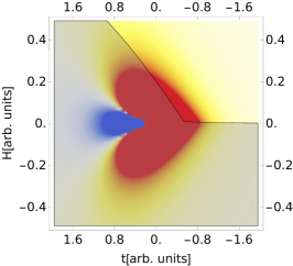
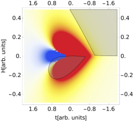
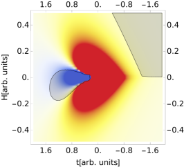
In Figs. (7a-7c) we show as the shaded areas the excluded regions around the critical point due to the conditions $C_{2}<0$, $C_{3}<0$, and $C_{4}>0$. Clearly the sign of the 2-particle correlation function, $C_{2}$, imposes the strongest constraint. In a sense this is good news, since the experimental determination of the two particle correlation function requires the least statistics as it requires only the measurement of the variance of the proton distribution. In addition, the measurement of $C_{2}$ is less affected by systematic uncertainties than higher order correlations, which probe the tails of the distribution. Also, one would expect that the aforementioned dynamical effects are likely to be better controlled and accounted for in case of the two particle correlations.

In conclusion, our schematic study showed that the signs of the correlations $C_{n}$ are a useful tool to exclude regions in the QCD phase diagram close to the critical point. The fact that the sign of the two particle correlations impose the strongest constraint suggests that both experimental as well as theoretical work should first and foremost concentrate on the quantitative understanding of two particle correlations.

V Summary and Conclusions

In this paper we have extracted the two- three- and four-proton correlation functions based on preliminary data of the STAR collaboration. We have discussed how these correlation functions are expected to scale with centrality and rapidity under various assumptions. We found that (a) at the lowest beam energy of $7.7{\rm\,GeV}$ there are significant four-proton correlations. (b) At $19.9{\rm\,GeV}$ the fourth order cumulant is dominated by a negative two-particle correlation. (c) For the lowest energies the centrality dependence change from that of an independent source model to a “collective” one at $N_{\rm part}\simeq 200$. At roughly the same centrality the three- and four-proton couplings change sign, indicating a change in the underlying dynamics. (d) The preliminary data on the rapidity dependence of the cumulant ratio $K_{4}/K_{2}$ rules out short-range rapidity correlations and is consistent with long-range ($\Delta y>1$) correlations. (e) We looked at the energy dependence of the relative contributions to the fourth order cumulant, $K_{4}$ and found that, with an excursion at $62.4{\rm\,GeV}$ the scaled correlation are rather constant from $200{\rm\,GeV}$ down to $19.6{\rm\,GeV}$. At lower energies both the three and four-proton correlations show a significant energy dependence.

We also explored to which extend the signs of the correlations functions $C_{n}$ constraint allowed regions in the phase diagram close tho the critical point. We found that the strongest constraint arises from the two-particle correlations. This suggests that both experimental as well as theoretical work should first focus on the quantitative understanding of the two particle correlations.

Finally, we should stress that the present analysis is based on preliminary data. Furthermore, one should not forget that there are sources of correlations other that critical dynamics. These need to be removed and understood, and we believe that a study of correlations functions, preferably differential in some of their variables, will be essential to make progress in the search for a QCD critical point.

Appendix A Correlation functions

Here we derive formulas for the couplings of the multi-particle genuine correlation functions for the case of protons and anti-protons. Let $P(N,\bar{N})$ denotes the multiplicity distribution of protons, $N$, and antiprotons, $\bar{N}$. The factorial moment generating function is given by

$$H(z,\bar{z})=\sum\nolimits_{N}\sum\nolimits_{\bar{N}}P(N,\bar{N})z^{N}\bar{z}^{\bar{N}}.$$ (43)

The factorial moments are given by

$$F_{i,k}\equiv\left\langle\frac{N!}{(N-i)!}\frac{\bar{N}!}{(\bar{N}-k)!}\right\rangle=\left.\frac{d^{i}}{dz^{i}}\frac{d^{k}}{d\bar{z}^{k}}H(z,\bar{z})\right|_{z=1,\bar{z}=1}.$$ (44)

The correlation function generating function is given by

$$G(z,\bar{z})=\ln\left[H(z,\bar{z})\right],$$ (45)

and

$$C_{n+m}^{(n,m)} = \int C_{n+m}^{(n,m)}(y_{1},\ldots,y_{n},\bar{y}_{1},...,\bar{y}_{m})dy_{1}\cdots dy_{n}d\bar{y}_{1}\cdots d\bar{y}_{m}$$ (46)

$$= \left.\frac{d^{n}}{dz^{n}}\frac{d^{m}}{d\bar{z}^{m}}G(z,\bar{z})\right|_{z=1,\bar{z}=1},$$

where $C_{n+m}^{(n,m)}$ is $n+m$ correlation function with $n$ protons and $m$ anti-protons. When we have only protons we have $C_{n}\equiv C_{n+0}^{(n,0)}$.

Performing straightforward calculations we obtain:

$$C_{2}^{(2,0)} = -F_{1,0}^{2}+F_{2,0}$$ (47)

$$C_{2}^{(1,1)} = -F_{0,1}F_{1,0}+F_{1,1}$$

$$C_{3}^{(3,0)} = 2F_{1,0}^{3}-3F_{1,0}F_{2,0}+F_{3,0}$$

$$C_{3}^{(2,1)} = 2F_{0,1}F_{1,0}^{2}-2F_{1,0}F_{1,1}-F_{0,1}F_{2,0}+F_{2,1}$$

$$C_{4}^{(4,0)} = -6F_{1,0}^{4}+12F_{1,0}^{2}F_{2,0}-3F_{2,0}^{2}-4F_{1,0}F_{3,0}+F_{4,0}$$

$$C_{4}^{(3,1)} = -6F_{0,1}F_{1,0}^{3}+6F_{1,0}^{2}F_{1,1}+6F_{0,1}F_{1,0}F_{2,0}-3F_{1,1}F_{2,0}-3F_{1,0}F_{2,1}-F_{0,1}F_{3,0}+F_{3,1}$$

$$C_{4}^{(2,2)} = (-6F_{0,1}^{2}+2F_{0,2})F_{1,0}^{2}+8F_{0,1}F_{1,0}F_{1,1}-2F_{1,1}^{2}-2F_{1,0}F_{1,2}+(2F_{0,1}^{2}-F_{0,2})F_{2,0}-2F_{0,1}F_{2,1}+F_{2,2}$$

where $F_{1,0}=\langle N\rangle$, $F_{0,1}=\langle\bar{N}\rangle$. The remaining correlations $C_{n+m}^{(n,m)}$ for $m>n$ can be easily obtained by a simple change of indexes $F_{i,k}\rightarrow F_{k,i}$.

The above equations allow to express factorial moments through correlation functions. Using formulas for the cumulants, Ref. Bzdak and Koch (2012), we obtain

$$K_{2} = \left\langle N\right\rangle+\left\langle\bar{N}\right\rangle+C_{2}^{(2,0)}+C_{2}^{(0,2)}-2C_{2}^{(1,1)}$$ (48)

$$K_{3} = \left\langle N\right\rangle-\left\langle\bar{N}\right\rangle+3C_{2}^{(2,0)}-3C_{2}^{(0,2)}+C_{3}^{(3,0)}-C_{3}^{(0,3)}-3C_{3}^{(2,1)}+3C_{3}^{(1,2)}$$

$$K_{4} = \left\langle N\right\rangle+\left\langle\bar{N}\right\rangle+7C_{2}^{(2,0)}+7C_{2}^{(0,2)}-2C_{2}^{(1,1)}+6C_{3}^{(3,0)}+6C_{3}^{(0,3)}-6C_{3}^{(2,1)}-6C_{3}^{(1,2)}+$$

$$C_{4}^{(4,0)}+C_{4}^{(0,4)}-4C_{4}^{(3,1)}-4C_{4}^{(1,3)}+6C_{4}^{(2,2)}$$

Finally the reduced correlation functions or couplings are related to $C_{n+m}^{(n,m)}$ through

$$c_{n+m}^{(n,m)}=\frac{C_{n+m}^{(n,m)}}{\left\langle N\right\rangle^{n}\left\langle\bar{N}\right\rangle^{m}},$$ (49)

or

$$c_{n+m}^{(n,m)}=\frac{\int\rho_{1}\left(y_{1}\right)\cdots\rho_{1}\left(y_{n}\right)\rho_{1}\left(\bar{y}_{1}\right)\cdots\rho_{1}\left(\bar{y}_{m}\right)c_{n+m}^{(n,m)}(y_{1},\ldots,y_{n},\bar{y}_{1},...,\bar{y}_{m})dy_{1}\cdots dy_{n}d\bar{y}_{1}\cdots d\bar{y}_{m}}{\int\rho_{1}\left(y_{1}\right)\cdots\rho_{1}\left(y_{n}\right)\rho_{1}\left(\bar{y}_{1}\right)\cdots\rho_{1}\left(\bar{y}_{m}\right)dy_{1}\cdots dy_{n}d\bar{y}_{1}\cdots d\bar{y}_{m}}.$$ (50)

References

- Stephanov et al. (1998) M. A. Stephanov, K. Rajagopal, and E. V. Shuryak, Phys. Rev. Lett. 81, 4816 (1998) .
- Stephanov (2009) M. Stephanov, Phys.Rev.Lett. 102, 032301 (2009) .
- Skokov et al. (2011) V. Skokov, B. Friman, and K. Redlich, Phys.Rev. C83, 054904 (2011) .
- Friman et al. (2011) B. Friman, F. Karsch, K. Redlich, and V. Skokov, Eur.Phys.J. C71, 1694 (2011) .
- Kitazawa et al. (2014) M. Kitazawa, M. Asakawa, and H. Ono, Phys.Lett. B728, 386 (2014) .
- Adamczyk et al. (2014a) L. Adamczyk et al. (STAR), Phys. Rev. Lett. 112, 032302 (2014a) .
- Adamczyk et al. (2014b) L. Adamczyk et al. (STAR), Phys. Rev. Lett. 113, 092301 (2014b) .
- Koch (2010) V. Koch, in Relativistic Heavy Ion Physics, Landolt-Boernstein New Series I, Vol. 23, edited by R. Stock (Springer, Heidelberg, 2010) pp. 626–652 .
- Anticic et al. (2010) T. Anticic et al. (NA49), Phys. Rev. C81, 064907 (2010) .
- Anticic et al. (2015) T. Anticic et al. (NA49), Eur. Phys. J. C75, 587 (2015) .
- Luo (2015) X. Luo (STAR), Proceedings, 9th International Workshop on Critical Point and Onset of Deconfinement (CPOD 2014): Bielefeld, Germany, November 17-21, 2014, PoS CPOD2014, 019 (2015) .
- Ling and Stephanov (2016) B. Ling and M. A. Stephanov, Phys. Rev. C93, 034915 (2016) .
- Bzdak and Bozek (2016) A. Bzdak and P. Bozek, Phys. Rev. C93, 024903 (2016) .
- Bzdak and Koch (2012) A. Bzdak and V. Koch, Phys. Rev. C86, 044904 (2012) .
- Lisa et al. (2005) M. A. Lisa, S. Pratt, R. Soltz, and U. Wiedemann, Ann. Rev. Nucl. Part. Sci. 55, 357 (2005) .
- Bzdak et al. (2013) A. Bzdak, V. Koch, and V. Skokov, Phys. Rev. C87, 014901 (2013) .
- Xu (2014) N. Xu (STAR), Proceedings, 24th International Conference on Ultra-Relativistic Nucleus-Nucleus Collisions (Quark Matter 2014), Nucl. Phys. A931, 1 (2014) .
- Luo and Xu (2017) X. Luo and N. Xu, arXiv:1701.02105 [nucl-ex] .
- Nonaka and Asakawa (2005) C. Nonaka and M. Asakawa, Phys. Rev. C71, 044904 (2005) .
- Stephanov (2011) M. Stephanov, Phys.Rev.Lett. 107, 052301 (2011) .
- Hippert et al. (2016) M. Hippert, E. S. Fraga, and E. M. Santos, Phys. Rev. D93, 014029 (2016) .
- Mukherjee et al. (2015) S. Mukherjee, R. Venugopalan, and Y. Yin, Phys. Rev. C92, 034912 (2015) .
- Herold et al. (2016) C. Herold, M. Nahrgang, Y. Yan, and C. Kobdaj, Phys. Rev. C93, 021902 (2016) .
- Guida and Zinn-Justin (1997) R. Guida and J. Zinn-Justin, Nucl. Phys. B489, 626 (1997) .
- Schofield (1969) P. Schofield, Phys. Rev. Lett. 22, 606 (1969).