Thermalization rates in the one dimensional Hubbard model with next-to-nearest neighbor hopping
Abstract
We consider a fermionic Hubbard chain with an additional next-to-nearest neighbor hopping term. We study the thermalization rates of the quasi-momentum distribution function within a quantum Boltzmann equation approach. We find that the thermalization rates are proportional to the square of the next-to-nearest neighbor hopping: Even weak next-to-nearest neighbor hopping in addition to nearest neighbor hopping leads to thermalization in a two-particle scattering quantum Boltzmann equation in one dimension. We also investigate the temperature dependence of the thermalization rates, which away from half filling become exponentially small for small temperature of the final thermalized distribution.
I Introduction
Understanding thermalization in quantum systems is essential to determine whether an experimental setup can be described by equilibrium concepts. Experimentally, this question becomes particularly relevant in cold atomic gases where unitary time evolution of closed quantum many body systems can be observed because the decohering effect of the environment is negligible (or at least under control) for the relevant time scales Greiner et al. (2002); Kinoshita et al. (2006); Hofferberth et al. (2007); Bloch et al. (2008); Schreiber et al. (2015); Langen et al. (2015). The ground breaking experiment of Kinoshita et al. Kinoshita et al. (2006) was the starting point for an ongoing theoretical effort to understand thermalization of low dimensional quantum many body systems. Their work considered the nonequilibrium dynamics of a 1d Bose gas with point-like interaction. Leaving aside heating and loss effects, they did not observe thermalization on the longest time scales accessible in their 1d experiment, while they reported rapid thermalization for the 3d equivalent of their system. So one key theoretical question is to understand this difference between the thermalization behavior of one dimensional and higher dimensional quantum systems.
A theoretical investigation of this question first requires a definition of what one means by thermalization. Obviously, under unitary time evolution a pure state always remains a pure state and never becomes a mixed state as employed to describe a thermal ensemble.
Therefore a more useful definition of thermalization is that the expectation values of an experimentally relevant set of observables are described by thermal values. This is the definition used in our work and we will show thermalization in this sense with respect to a certain set of observables, namely the momentum distribution function.
Theoretical research in the past decade has revealed different thermalization behavior of integrable and non-integrable systems. While the notion of integrability in quantum systems is not uniquely defined (Caux and Mossel, 2011), these differences do not seem to play a role with respect to thermalization: The long-time limit of an initial state can be described (with respect to a relevant set of observables) as a generalized Gibbs ensemble that takes into account the expectation values of the conserved quantities of the integrable model Rigol et al. (2007). On the other hand, in non-integrable systems it has been shown that even a single eigenstate can be typical for an entire thermal ensemble in the sense that expectation values of few body observables are indistinguishable. This important observation regarding the foundations of quantum statistical mechanics is called eigenstate thermalization hypothesis (ETH) Deutsch (1991); Srednicki (1994); Rigol et al. (2008). Hence the question arises what happens at the transition from integrability to non-integrability. We will address this issue for a specific one-dimensional quantum system which is of paradigmatic importance for condensed-matter physics, namely the Hubbard model.
Studying the thermalization dynamics in 1d quantum systems explicitly is very challenging. For weak quantum quenches in higher spatial dimensions one generically expects three distinct time regimes: an initial buildup of quasiparticles, a prethermalized (Eckstein et al., 2009; Gring et al., 2012; Fagotti, 2014; Bertini and Fagotti, 2015) time regime (having non-thermal quasi-stationary states) and a long time thermalization described by a quantum Boltzmann-equation (QBE). This picture has been established by studying the quench dynamics of the Hubbard model for dimensions both analytically and numerically Moeckel and Kehrein (2008); Eckstein et al. (2009). In one dimension the general consensus is that the Boltzmann dynamics is ineffective for two particle scattering processes due to the simultaneous conservation of single particle energies and momenta. Therefore the thermalization time scale in one dimension is expected to be much longer (for example via multi particle scattering processes). Putting it otherwise, the prethermalized time regime will extend to much longer times.
This behavior is difficult to investigate numerically. Methods like t-DMRG are limited to not too large times due to the entanglement growthManmana et al. (2007), and exact diagonalization methods are intrinsically limited to small finite systems and require an extrapolation to infinite system size. A noteable exception is a recent paper by Bertini et al. Bertini et al. (2015), which uses a combination of numerical and analytical methods to show how the prethermalized regime evolves towards thermal equilibrium after a quench in a dimerized 1d model of spinless fermions. Similarly, in our work we want to contribute to understanding the thermalization behavior of 1d systems by giving an explicit estimate for the thermalization rate based on a QBE approach in the 1d fermionic Hubbard model. Specifically, we investigate the role of an additional next-to-nearest-neighbor-hopping-term (NNNH) which is tuned by the prefactor within a QBE approximation. While one sometimes finds the assertion that there is no thermalization from a Boltzmann equation with 2-particle scattering in one dimension, we find that this is not true in our model. This observation was already made by Fürst et al. Fürst et al. (2012, 2013a) and we elaborate on this initial finding systematically in this paper by deriving all thermalization rates within a linear approximation. Only for the case of nearest neighbor hopping only without next-to-nearest neighbor hopping does the system not thermalize, any nonvanishing next-to-nearest neighbor hopping leads to thermalization in the long time limit.
The article is structured as follows. In Sec. II we introduce our model, the 1d fermionic Hubbard model (FHM) with a next-to-nearest neighbor hopping term (NNNH), and our method, the quantum Boltzmann equation approach (QBE). We will use a linearized Boltzmann equation to find the relaxation times. Furthermore we will comment on the conserved quasi-momentum distribution (QMD) Fürst et al. (2012) in the standard FHM. Sec. III is devoted to our results and the conclusions are summed up in Sec. IV. App. A shows the stationarity of certain QMD s. We explain our numerics in App. B. App. D is about constructing a generalized Gibbs ensemble (GGE) at low temperatures.
II Model and method
II.1 Model
We consider the Fermi-Hubbard model (FHM) with an additional NNNH,
| (1) | ||||
Measuring energies in units of the hopping , we define dimensionless parameters and . will denote the final temperature of the thermalized state, which is therefore determined by the energy of the initial state. Obviously implies that the initial state is the ground state.
The dispersion relation of our model is
| (2) |
It is measured in units of , such that the kinetic energy is and the dimensionless inverse temperature is .
II.2 Boltzmann-Equation
A QBE describes the long time behavior of the QMD Erdös et al. (2004); Fürst et al. (2012, 2013a, 2013b)
| (3) |
Here we defined the expectation value . We assume the initial state to satisfy restricted quasi-freeness. This means that there is a (approximate) Wick theorem for the 4-point and 6-point functions. The QBE is valid on kinetic time scales(Fürst et al., 2013b), i.e. times of . We operate under the normal assumption that the Boltzmann-description is still valid on longer times.
This time evolution was previously investigated by Fürst et al (Fürst et al., 2012, 2013a) for some initial states. They found that for , the system runs into a non-thermal stationary state. However, for they have seen that their initial states thermalize. The thermalization times they found for small were much larger than the relaxation times for the case.
The QBE is
| (4) |
The collision term is a non-linear operator that depends on the QMD . Thus is a function of and . We use the QBE of Fürst et al. (2012) for the 1d FHM. We restrict ourselves to the spin-symmetric case in which - and -spin fermions have the same QMD,
| (5) |
In the spin symmetric case we can also assume
| (6) |
We obtain the collision term
| (7) |
Here we introduced the notation . is the change in energy and the change in total momentum. The sum over allows for Umklapp processes. The matrix element of the Fermi-Hubbard-interaction simply leads to the prefactor . The prefactor’s time scale is . For a typical half bandwidth of this timescale is .
Note that the Fermi-Dirac distribution makes the collision term vanish, as can be verified easily. This corresponds to the well-known fact that thermal distributions are fixed points of the Boltzmann equation.
Also note that the applicability of the quantum Boltzmann equation relies on fermionic quasiparticle lifetimes of order or larger than the scattering time. In the one dimensional Hubbard model the appropriate quasiparticles are bosonic (spinons and holons). However, if their velocities do not differ much one can still use the fermionic quasiparticle picture for not too long times, which provides the justification for our approach.
II.3 Dispersion relations
The QBE describes time evolution due to 2-particle-collisions. The ability of thermalization due to 2-particle-collisions strongly depends on the dispersion relation . For instance, if it was quadratic, i.e. , momentum conservation and energy conservation lead to the following constraints on the 2-particle-collision:
| (8) |
This is equivalent to
| (9) |
These are two trivial scattering channels. This means that the collision term is zero, i.e. these interaction-channels do not change the QMD. All dispersion relations permit these trivial channels. While other dispersion relations like nearest-neighbor hopping, , allow additional scattering processes, the general consensus in the literature is that in one dimension these additional scattering processes are not sufficient to lead to thermalization. However, building on the work of Fürst et al. Fürst et al. (2012, 2013a), we will show systematically that adding a next-to-nearest-neighbor hopping term does indeed lead to thermalization from two particle scattering, contrary to that often stated opinion in the literature.
II.4 Linearization
We want to find the relaxation rates. Therefore we linearize the QBE around its thermal distribution, the Fermi-Dirac distribution
| (10) |
This approximation becomes exact in the limit of small perturbations around the thermal distribution: We will show that asymptotically a thermal distribution is reached, which therefore provides an a posteriori justification for the linearization. Hence we obtain the exact time scales describing the late time approach to the thermal distribution. The linearization worked out in this subsection follows the scheme described in Haug and Jauho (1996). We start out by introducing a perturbation that we put into the exponent of the Fermi-Dirac distribution:
| (11) | ||||
This ansatz has two advantages over the naive scheme . First one does not have to care so much about the magnitude of . In the naive scheme one would have to require . For us instead it is sufficient to assume . The second advantage a much better numerical stability for low temperatures.
Plugging Eq. 11 into the QBE in Eq. 4, we get a rate equation for the perturbation using the stationarity of the Fermi-Dirac distribution, :
| (12) |
Here we have neglected higher order terms in the perturbation , so from now on we can work with the linear operator .
II.5 Expansion in eigenfunctions
This linear operator is positive semi-definite and Hermitian with respect to the scalar product
| (13) |
which induces the norm . The eigenfunctions of are denoted by and the associated eigenvalues by . We expand the perturbation in using and find
| (14) |
The coefficients are determined by the initial perturbation . They measure the contribution of the eigenfunction to the perturbation . The exponential factor shows that the are the rates we are looking for. Due to the fact, that is positive semi-definite, the eigenvalues are non-negative and we order them by size, .
If an eigenvalue is zero, its corresponding contribution to the perturbation persists for all times. There are two eigenvalues which are always zero:
| (15) |
They correspond to the eigenfunctions and . A nonzero contribution from these eigenfunctions in our perturbation simply changes the temperature and the chemical potential according to Eq. 11:
| (16) | ||||
Therefore these two eigenvalues do not set the thermalization rate: we can eliminate their contributions and by using the correct final temperature and chemical potential in Eq. 11. Thus it is the eigenvalue which sets the thermalization rate if the initial perturbation has nonzero overlap with the corresponding eigenvector, . In general the first eigenvalue , with sets the thermalization rate. We will later see that this is important when approaching half filling because shows very different behavior from . So its respective eigenfunction will be of special interest.
II.6 Stationary distributions
In the integrable case with nearest-neighbor-hopping only, , Fürst et al. Fürst et al. (2012) found non-thermal stationary QMD s. These distributions have the form
| (17) |
where is antisymmetric around and is arbitrary. This means that the are stationary perturbations for and the corresponding eigenvalues of the linearized Boltzmann operator vanish.
One can immediately see that all these form a connected subspace of , i.e. the can be smoothly transformed into each other. Obviously the thermal QMD s also belong to this subspace. For we expect these eigenvectors to change in order , i.e. . Furthermore we expect them to become long lived and eventually decay to a thermal QMD. We denote these quasi-stationary as well as their associated stationary distributions (for ) as “quasi-stationary QMD” (QSQMD). They turn out to have the (slightly broken) symmetry
| (18) |
An arbitrary initial QMD will relax into a QSQMD on short time scales. For it will then slowly flow to the respective thermal QMD.
For later reference, Ref. Fürst et al. (2012) found that for the only processes that contribute in the QBE fulfill . For small this constraint becomes
| (19) |
For larger next-to-nearest-neighbor hopping, , there is an additional interaction channel. In this work we restrict ourselves to , where only one interaction channel has to be considered.
III Results
III.1 Relaxation rates
In order to obtain the relaxation rates we first compute a discretized version of the operator . The main difficulty is that a careful interpolation needs to be performed in order to achieve high accuracy. The reason for this is that energy conservation makes it necessary to evaluate the perturbation between grid-points of the discretization. Then we diagonalize the discretized operator and perform a finite size scaling analysis of the eigenvalues. A detailed description of the numerics is given in App. B.
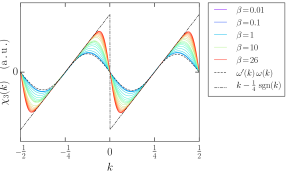
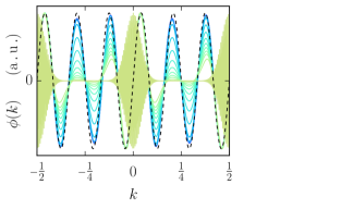
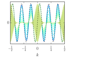
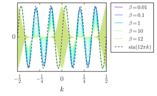
First of all we verify some analytical facts mentioned above. The first two eigenvalues are at least about times smaller than the largest eigenvalue. As expected from the discussion in Sec. II.5, the corresponding eigenfunctions are superpositions of the constant function and the dispersion relation. Figs. 1 and 2 show eigenfunctions of correspoding to low lying (nonvanishing) eigenvalues. They are antisymmetric around up to a correction of . So they have the correct symmetry as given by Eq. 18 to be a perturbation corresponding to a QSQMD.
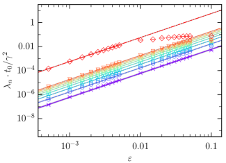
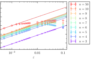
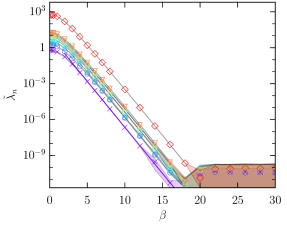
The two double logarithmic plots in Fig. 3 show the lowest non-zero eigenvalues for and . Plotted are the eigenvalues after extrapolating to an infinitesimal discretization grid of the linearized Boltzmann operator. The lines are fits with a quadratic -dependence. For the fits we only used points in the -regime of the eigenvalues. These fits show that for sufficiently small every low lying eigenvalue has a quadratic dependence on the relative strength to the next-to-nearest-neighbor hopping. Fig. 3 also shows that the linear fits are an upper bound to their respective eigenvalue.
From this data we can already conclude that nearest-neighbor hopping plus nonvanishing next-to-nearest-neighbor hopping is indeed sufficient to achieve thermalization via two particle scattering in one dimension. The thermalization rates are quadratic in the relative strength of the next-to-nearest-neighbor hopping (for small ).
Similar data like in Fig. 3 was obtained for chemical potentials and for the inverse final temperature ranging from to . In all cases the eigenvalues are proportional to for sufficiently small , so the lowest non-zero eigenvalues obey
| (20) |
for and sufficiently small. Here are the proportionality factors which we will denote “rescaled eigenvalues”. One can also show analytically that there are no terms proportional to .

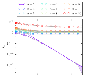
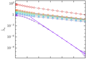
Fig. 4 shows three plots depicting the rescaled eigenvalues as functions of . The first non-zero eigenvalue decreases exponentially as a function of inverse temperature for all fillings. The higher eigenvalues () decay exponentially away from half filling, but are asymptotically constant for at half filling. The straight lines are fits to exponential behavior which we can parametrize as
| (21) |
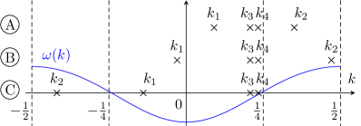
This behavior can be explained by Umklapp processes (see also Ref. Rosch and Andrei (2000)). At half filling the situation is shown in Fig. 5. Consider for example two particles with momenta . They can scatter into and . The latter becomes by subtraction of the reciprocal lattice vector. This process becomes less likely away from half filling. The Fermi points shift apart (or together) when changing the filling and Umklapp processes like the one depicted in Fig. 5 cannot happen any more. Therefore Umklapp processes are most effective at half filling for low final temperatures.
Therefore generically thermalization becomes exponentially slow as a function of the inverse final temperature (equivalently: the inverse initial excitation energy) away from half filling. At half filling only the eigenvector shows this behavior, so at half filling there is no exponential slowdown of thermalization as a function of inverse final temperature if the initial perturbation does not couple to this eigenvector. Therefore this eigenvalue and its eigenfunction are of special interest. The next sections will deal with understanding this eigenfunction .
III.2 Structure of
The values of the initial perturbation around and are not important for small temperatures since they are suppressed by the factor , see Eq. 11. So based on Fig. 1 a good approximation of the third eigenfunction is given by
| (22) |
This is shown in Fig. 6. One can see that approaches zero in the limit , which means that indeed is a good approximation. Using this result one can show App. C that Umklapp and forward scattering do not contribute in , only backscattering can occur. But backscattering is limited to being in the vicinity of or , which leads to the exponential suppression of as a function of inverse temperature App. C.
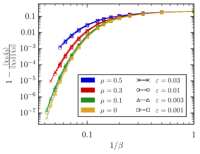
In the following we consider two operators which have a connection to . The first operator, , comes from the approximate eigenfunction . The other operator will turn out to be the total energy current operator .
Let us first construct operators in state space using the eigenfunctions of :
| (23) |
Their expectation values are
| (24) | ||||
where . Since is proportional to this indicates if there is a slowly decaying perturbation in the system.
An operator can be used for the construction of a generalized Gibbs ensemble (GGE) that describes the long time limit of the QMD provided that . For the integrable case, , there are infinitely many zero eigenvalues and therefore an infinite number of conserved charges that enter such a GGE.
Now we consider specifically . As discussed above, the eigenvalue is very small for low final temperatures. So may be used for the construction of a GGE (see App. D), that describes the QMD on time scales . In order to give the the operator a physical meaning, we replace with its approximation , Eq. 22:
| (25) |
with the constant . The momentum term of leads to the total momentum operator , the signum function results in the operator . Here counts the particle number on the left side of the Brioullin zone, and the particle number on the right side. The reason for the long living expectation value of is the same as for the approximate stationarity of : Umklapp processes are ineffective even at half filling.
Long living currents:
On times the perturbation has decayed to and its exponential factor is still approximately one. Fig. 1 shows that is asymmetric around . So the corresponding momentum distribution is also asymmetric corresponding to nonvanishing currents. The operators of the total particle and energy current are
| (26) |
respectively. The local current operators and fulfill a discretized version of the continuity equation. is simply the group velocity and also includes the dispersion relation. Following the scheme in Eq. 24, the expectation values evaluate to
| (27) |
One can show numerically and analytically that is not zero. Notice that the right hand side of Eq. 27 is independent of system size, as is the left hand side. Therefore there are long living currents if one creates an initial perturbation that fulfills .
IV Conclusions
We have investigated the long time behavior of the quasi-momentum distribution of a one-dimensional fermionic Hubbard model with additional next-to-nearest-neighbor hopping . Using a linearized Boltzmann equation we could systematically verify that thermalization occurs from two particle scattering processes if is nonzero Fürst et al. (2012, 2013a). It is often stated that a Boltzmann equation with two particle scattering is ineffective in one dimension because of simultaneous energy and momentum conservation. Following Fürst et al. Fürst et al. (2012, 2013a) we have therefore verified that this statement is incorrect for a band dispersion described by nearest neighbor plus next-to-nearest-neighbor hopping.
Away from half filling the relaxation rates are quadratic in the relative strength of the next-to-nearest-neighbor hopping and are exponentially suppressed as a function of inverse final temperature. This implies that thermalization occurs, but on an exponentially increasing time scale for low excitation energy of the initial perturbation. At half filling this picture is different since Umklapp processes play an important role even at low temperatures: at half filling the only perturbation with such an exponential slowdown corresponds to the current, all other perturbations decay with a constant rate (still proportional to ) in the low temperature limit. Notice the difference to the behavior predicted by the QBE in higher dimensions where the smallest relaxation rates are proportional to .(Kabanov and Alexandrov, 2008) In a pump-probe experiment this would translate into a much stronger (exponential) dependence of the thermalization time scale on fluence in one dimension.
V Acknowledgments
We thank H. Spohn, A. Mitra, G. Mussardo, M. Medvedyeva, I. Homrighausen, D. Fioretto, R. Härtle, and S. R. Manmana for helpful discussions. This work was supported by the SFB1073 (project B03) of the Deutsche Forschungsgemeinschaft (DFG).
Appendix A Stationary distributions of the standard FHM
Appendix B Numerics
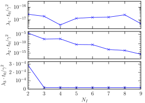

To get the thermalization rates we need to find the eigenvalues of . Therefore we discretize the operator, diagonalize it and extrapolate its spectrum to the continuum limit.
We discretize by discretizing momentum space:
| (30) |
The discretized operator is denoted by the matrix , the discretized perturbation by the vector :
| (31) |
Then we need to obtain the non-trivial solutions of . It can be shown that for every there is exactly one non-trivial solution as long as . This is because the dispersion relation is symmetric around zero, monotonic in the interval , and periodic. We numerically calculate the solutions by a Newton-Raphson procedure. In general these solutions are not on the grid . But considering the formula for , Eq. 12, we realize that the perturbation has to be evaluated at . This can only be done with an interpolation of the discretized perturbation .
This is why we have to use an interpolation scheme to evaluate . A naive interpolation, like using step functions or linear functions, leads to large errors. So we use
| (32) | ||||
where is the number of interpolation momenta, are the nearest discretized momenta next to and the respective weights. These weights are calculated such that is approximated in the best possible way. In our case there is exactly one solution for a given tuple . This is why the sum over is dropped in the last line of Eq. Eq. 32.
Using our interpolation scheme for we obtain
| (33) |
For our purposes we found that is a reasonable choice. The speed of the numerical evaluation is still fast enough while providing high precision. This is shown in Fig. 7. There we plotted the first three eigenvalues. is fluctuating around . The reason is the simple nature of its corresponding eigenfunction . It is an exact eigenfunction for any discretization in our numerics due to the fact that trivially. So measures the resolution of zero. The eigenfunction , however, is curved and therefore the numerical eigenfunction is influenced by the interpolation scheme. Thus measures the numerical precision including the interpolation scheme. Additionally we plotted in Fig. 7 as a reference for the other eigenvalues. One can see that from on it does not change any more and becomes independent of our interpolation scheme.
The eigenvalues of are found by exact diagonalization. These are then extrapolated to to obtain the eigenvalues of , see Fig. 8. Figs. 8A and B show that for lower oscillations are visible for the lower eigenvalues. But for higher (like in C) these oscillations disappear. However, always shows a strong exponential decay towards . So one has to cover a variety of extrapolations. Therefore we use a script, which extrapolates our data for several , and . It fits a constant function, an exponential function and the function to the data. Then the script chooses the one with the smallest error (straight lines). The value at as well as the error are used to create the plots in Fig. 3.
Appendix C Scattering processes for
In Sec. III.2 we consider to explain the smallness of the eigenvalue corresponding to the eigenfunction . In order to do that we need two ingredients. Note that both apply to all eigenfunctions. The first one is the fact that the mean momentum lies in an -region around , see Eq. 19. The second ingredient is the structure of , which contains all the Fermi functions:
| (34) | ||||
For away from full or empty filling both Eqs. 19 and 34 make and lie on the same side of the Brioullin zone. This means that either both are positive or both are negative. Since we only explain the linear regions of , is away from and . This and Eq. 19 make also and lie on the same side of the Brioullin zone. Thus in with around there is no backward scattering like Fig. 9B. There is only forward and Umklapp scattering like illustrated in Fig. 9A and C, respectively.
Now we use the linear form of and consider the factor
| (35) |
in . The approximate eigenfunction , see Eq. 22, consists of two terms. These are the momentum or identity function and the signum function . We calculate Eq. 35 for both functions separately.
First we consider forward scattering, i.e. all have the same sign, see e.g. Fig. 9A. Plugging the momentum function into Eq. 35 gives because forward scattering processes obey momentum conservation. Plugging the signum function into Eq. 35 gives zero, too. So forward scattering does not contribute to .
Now we consider Umklapp scattering, see e.g. Fig. 9C. There momentum is not conserved. Thus plugging the momentum function into Eq. 35 we obtain the momentum change . It is compensated by the signum function plugged into Eq. 35: . This has the same sign as the momentum change, which leads to cancellation in Eq. 35. This explains the signum function’s prefactor of in the approximate eigenfunction. So Umklapp scattering does not contribute to , similar to forward scattering.
Appendix D GGE for
In Sec. II.4 we learned that the first non-trivial eigenvalue is . In Fig. 1 we saw that for the associated eigenfunction approaches . In the following we derive the respective (approximately) conserved quantity. The generalized Gibbs ensemble (GGE) is
| (36) |
The conserved quantity has the form
| (37) |
We find
| (38) |
analogous to the standard text book derivation of the Fermi-Dirac-distribution. Comparing this to Eq. 11, where we defined our linearization of , we identify . Therefore
| (39) | ||||
Note that the factor does not depend on . It is due to the fact that has to be antisymmetric around for a quasi-stationary state, see Sec. II.6.
References
- Greiner et al. (2002) M. Greiner, O. Mandel, T. W. Hänsch, and I. Bloch, Nature 419, 51 (2002).
- Kinoshita et al. (2006) T. Kinoshita, T. Wenger, and D. S. Weiss, Nature 440, 900 (2006).
- Hofferberth et al. (2007) S. Hofferberth, I. Lesanovsky, B. Fischer, T. Schumm, and J. Schmiedmayer, Nature 449, 324 (2007).
- Bloch et al. (2008) I. Bloch, J. Dalibard, and W. Zwerger, Rev. Mod. Phys. 80, 885 (2008).
- Schreiber et al. (2015) M. Schreiber, S. S. Hodgman, P. Bordia, H. P. Lüschen, M. H. Fischer, R. Vosk, E. Altman, U. Schneider, and I. Bloch, Science 349, 842 (2015).
- Langen et al. (2015) T. Langen, S. Erne, R. Geiger, B. Rauer, T. Schweigler, M. Kuhnert, W. Rohringer, I. E. Mazets, T. Gasenzer, and J. Schmiedmayer, Science 348, 207 (2015).
- Caux and Mossel (2011) J.-S. Caux and J. Mossel, Journal of Statistical Mechanics: Theory and Experiment 2011, P02023 (2011).
- Rigol et al. (2007) M. Rigol, V. Dunjko, V. Yurovsky, and M. Olshanii, Phys. Rev. Lett. 98, 050405 (2007).
- Deutsch (1991) J. M. Deutsch, Phys. Rev. A 43, 2046 (1991).
- Srednicki (1994) M. Srednicki, Phys. Rev. E 50, 888 (1994).
- Rigol et al. (2008) M. Rigol, V. Dunjko, and M. Olshanii, Nature 452, 854 (2008).
- Eckstein et al. (2009) M. Eckstein, M. Kollar, and P. Werner, Phys. Rev. Lett. 103, 056403 (2009).
- Gring et al. (2012) M. Gring, M. Kuhnert, T. Langen, T. Kitagawa, B. Rauer, M. Schreitl, I. Mazets, D. A. Smith, E. Demler, and J. Schmiedmayer, Science 337, 1318 (2012), http://science.sciencemag.org/content/337/6100/1318.full.pdf .
- Fagotti (2014) M. Fagotti, Journal of Statistical Mechanics: Theory and Experiment 2014, P03016 (2014).
- Bertini and Fagotti (2015) B. Bertini and M. Fagotti, Journal of Statistical Mechanics: Theory and Experiment 2015, P07012 (2015).
- Moeckel and Kehrein (2008) M. Moeckel and S. Kehrein, Phys. Rev. Lett. 100, 175702 (2008).
- Manmana et al. (2007) S. R. Manmana, S. Wessel, R. M. Noack, and A. Muramatsu, Phys. Rev. Lett. 98, 210405 (2007).
- Bertini et al. (2015) B. Bertini, F. H. L. Essler, S. Groha, and N. J. Robinson, Phys. Rev. Lett. 115, 180601 (2015).
- Fürst et al. (2012) M. L. R. Fürst, C. B. Mendl, and H. Spohn, Phys. Rev. E 86, 031122 (2012).
- Fürst et al. (2013a) M. L. R. Fürst, C. B. Mendl, and H. Spohn, Phys. Rev. E 88, 012108 (2013a).
- Erdös et al. (2004) L. Erdös, M. Salmhofer, and H.-T. Yau, Journal of Statistical Physics 116, 367 (2004).
- Fürst et al. (2013b) M. L. R. Fürst, J. Lukkarinen, P. Mei, and H. Spohn, Journal of Physics A: Mathematical and Theoretical 46, 485002 (2013b).
- Haug and Jauho (1996) H. Haug and A.-P. Jauho, Quantum Kinetics in Transport and Optics of Semiconductors (Springer, 1996).
- Rosch and Andrei (2000) A. Rosch and N. Andrei, Phys. Rev. Lett. 85, 1092 (2000).
- Kabanov and Alexandrov (2008) V. V. Kabanov and A. S. Alexandrov, Phys. Rev. B 78, 174514 (2008).