Non-perturbative determination of improvement coefficients using coordinate space correlators in $N_{f}=2+1$ lattice QCD

Abstract

We determine quark mass dependent order $a$ improvement terms of the form $b_{J}am$ for non-singlet scalar, pseudoscalar, vector and axialvector currents using correlators in coordinate space on a set of CLS ensembles. These have been generated employing non-perturbatively improved Wilson Fermions and the tree-level Lüscher-Weisz gauge action at $\beta=3.4,3.46,3.55$ and $3.7$, corresponding to lattice spacings ranging from $a\approx 0.085\,\textmd{fm}$ down to $0.05\,\textmd{fm}$. In the $N_{f}=2+1$ flavour theory two types of improvement coefficients exist: $b_{J}$, proportional to non-singlet quark mass combinations, and $\bar{b}_{J}$ (or $\tilde{b}_{J}$), proportional to the trace of the quark mass matrix. Combining our non-perturbative determinations with perturbative results, we quote Padé approximants parameterizing the $b_{J}$ improvement coefficients within the above window of lattice spacings. We also give preliminary results for $\tilde{b}_{J}$ at $\beta=3.4$.

I Introduction

Lattice simulations of quantum chromodynamics (Lattice QCD) have become an indispensable tool in particle and hadron physics phenomenology. By discretizing a quantum field theory on a lattice with a spacing $a>0$, ultraviolet divergences are regularized. At the same time this enables the numerical simulation of QCD, including its non-perturbative dynamics. In principle such simulations need to be performed for different values of the lattice spacing, in order to remove the regulator by taking the continuum limit, $a\rightarrow 0$. In QCD this limit is approached as a polynomial in $a$, modulated by logarithmic corrections.

Obviously, many possible discretizations of the quark (and gluon) parts of the action exist. Staggered quarks suffer from conceptional problems, unless all Fermions come in mass degenerate groups of four flavours. Also combining the flavour and spin degrees of freedom complicates operator mixing and the analysis of two- and three-point Green functions. Domain wall and overlap actions have the most desirable theoretical properties as even at a non-vanishing value of the lattice spacing these possess an (almost) exact chiral symmetry in the massless limit. In contrast, using Wilson Fermions, chiral symmetry only becomes restored in the continuum limit, and also an additive mass renormalization is encountered. Wilson Fermions, however, are computationally much less expensive to simulate and therefore offer the possibility of obtaining results at several values of the lattice spacing, enabling a controlled continuum limit extrapolation.

Unlike other Fermion discretizations, where leading lattice artefacts are of order $a^{2}$, for naive Wilson Fermions these are linear in $a$. Such terms can, however, be removed non-perturbatively Luscher:1996sc ; Luscher:1996ug , Symanzik improving Symanzik:1983dc the action and the local operators of interest. Recently, within the Coordinated Lattice Simulations (CLS) effort Bruno:2014jqa , we embarked on a large scale simulation programme, employing $N_{f}=2+1$ flavours of order $a$ improved Wilson-Sheikholeslami-Wohlert Sheikholeslami:1985ij (clover) Fermions and the tree-level improved Lüscher-Weisz gauge action Weisz:1982zw ; Luscher:1984xn . CLS use open boundary conditions in time Luscher:2011kk , thereby increasing the mobility of topological charges and enabling us to maintain ergodicity at finer lattice spacings than had been possible previously. For details on the action, ensembles and parameter values, see Ref. Bruno:2014jqa .

As the cost of simulations increases with a large inverse power of the lattice spacing, we aim at not only order $a$ improving the action but also all operators that will appear in matrix elements of interest. It is important to remove such contributions, that are linear in $a$, non-perturbatively since terms of order $g^{2\nu}a$, where $g$ denotes the gauge coupling, will survive a $(\nu-1)$-loop perturbative subtraction. As $g^{2}$ varies only slowly with $a$, close to the continuum limit any $g^{2\nu}a$ term will dominate over $a^{2}$ terms. The non-perturbative improvement of the action and of the massless axial current was carried out in Refs. Bulava:2013cta ; Bulava:2015bxa . In addition to such “$c_{J}$” improvement terms that persist in the massless limit, in the massive case additional $b_{J}$ and $\bar{b}_{J}$ coefficients are encountered for a current $J$, for definitions, see, e.g., Ref. Bhattacharya:2005rb . Existing results as of 2006 are reviewed in Ref. Sommer:2006sj and, more recently, for $N_{f}=2$ clover quarks on Wilson glue, the combinations $b_{A}-b_{P}$ and $b_{S}=-2b_{m}$ were determined non-perturbatively in Ref. Fritzsch:2010aw .

Here we introduce a variant of the coordinate space method that was originally proposed in Ref. Martinelli:1997zc . This will allow us to determine the scalar, pseudoscalar, vector and axial $b_{J}$ coefficients, accompanying both flavour-singlet and non-singlet quark mass combinations, with very limited computational effort. This is then successfully applied to the CLS ensembles described above.

This article is organized as follows. In Sec. II we describe the general approach and define the observables that will be studied. Next, in Sec. III we analyse these observables at tree-level in lattice and continuum perturbation theory, including the leading non-perturbative effects, that are expected from the operator product expansion. This will allow us to improve the observables, to estimate the size of cut-off effects and to select the optimal set of separations at which the correlation functions are evaluated in the non-perturbative study. Then in Sec. IV we discuss systematic errors of our approach, addressing finite volume effects and estimating contributions of non-perturbative condensates. Finally, in Sec. V we present results for all order $am$ coefficients. In Sec. VI we conclude and present an outlook.

II Description of the method

We generalize the method of Ref. Martinelli:1997zc to the situation of $N_{f}=2+1$ non-degenerate quark mass flavours. For increased precision, we perturbatively subtract the leading order lattice artefacts. Furthermore, we employ the operator product expansion (OPE), enabling us to quantitatively describe medium distance corrections.

We will assume improved Wilson quarks and — as we aim at order $a$ improvement — we will consequently drop all terms of order $a^{2}$. We remark that different prescriptions of obtaining improvement coefficients will in general give results that differ by such higher order corrections.

We denote quark mass averages following Refs. Bali:2016umi ; Bhattacharya:2005rb as

$$m_{jk}=\frac{1}{2}(m_{j}+m_{k})\,,$$ (1)

where

$$m_{j}=\frac{1}{2a}\left(\frac{1}{\kappa_{j}}-\frac{1}{\kappa_{\textrm{crit}}}\right).$$ (2)

The critical hopping parameter value $\kappa_{\textrm{crit}}$ is defined as the point where the axial Ward identity (AWI) quark mass vanishes in the theory with $N_{f}=3$ mass degenerate quark flavours.

We will label the mass of the two degenerate quark flavours as $m_{1}=m_{2}=m_{\ell}$ and the mass of the remaining (strange) quark as $m_{3}=m_{s}$. The mass dependence of physical observables can be parameterized in terms of the average quark mass

$$\overline{m}=\frac{1}{3}\left(m_{s}+2m_{\ell}\right)\,,$$ (3)

and the light quark mass $m_{12}$ or, equivalently, the average of the strange and light quark masses $m_{13}$: if $\overline{m}$ and either $m_{12}$ or $m_{13}$ are known, $m_{\ell}$ and $m_{s}$ are fixed. Most ensembles have been generated following the strategy of the QCDSF Collaboration Bietenholz:2010jr , keeping $\overline{m}$ constant. This is supplemented by further ensembles at an (approximately) fixed value of the renormalized strange quark mass, as well as along the symmetric line $m_{\ell}=m_{s}$ Bali:2016umi .

II.1 General considerations and definitions

We define connected Euclidean current-current correlation functions in a continuum renormalization scheme $R$, e.g., $R=\overline{\mathrm{MS}}$, at a scale $\mu$:

$$G_{J^{(jk)}}^{R}(x,m_{\ell},m_{s};\mu)=\left\langle\Omega\left|T\,J^{(jk)}(x)\overline{J}^{(jk)}(0)\right|\Omega\right\rangle^{R}.$$ (4)

$T$ denotes the time ordering operator, which we shall omit below as path integral expectation values are automatically time ordered. $|\Omega\rangle$ is the vacuum state and $J\in\{S,P,V_{\mu},A_{\mu}\}$. The current is defined as

$$J^{(jk)}=\overline{\psi}_{j}\Gamma_{J}\psi_{k}\,,\quad\overline{J}^{(jk)}=\overline{\psi}_{k}\Gamma_{J}^{\dagger}\psi_{j}\,,$$ (5)

with $\Gamma_{J}\in\{\mathds{1},\gamma_{5},\gamma_{\mu},\gamma_{\mu}\gamma_{5}\}$. $\psi_{j}$ destroys a quark of flavour $j\in\{1,2,3\}$ and $x$ is a four-distance vector in coordinate space. As here we will only consider flavour non-singlet currents, we always assume $j\neq k$.

The above correlation function differs from that of the massless case by mass dependent terms Reinders:1981sy ; Reinders:1984sr ; Jamin:1992se ,

$$G_{J^{(jk)}}^{R}(x,m_{\ell},m_{s};\mu)=G_{J^{(jk)}}^{R}(x,0,0;\mu)$$ (6)

$$\times \left[1+\mathcal{O}\left(m^{2}x^{2},m^{2}\langle FF\rangle x^{6},m\langle\overline{\psi}\psi\rangle x^{4},m\langle\overline{\psi}\sigma F\psi\rangle x^{6}\right)\right]\,,$$

where at each order in $m$ we only display the dominant type of term. Note that only even powers of $x$ can appear above. Regarding the non-perturbative correction terms, the light quark condensate (in the $\overline{\mathrm{MS}}$ scheme at the scale $\mu=2\,\textmd{GeV}$) reads $\langle\overline{\psi}\psi\rangle=-\Sigma_{0}=-[274(3)\,\textmd{MeV}]^{3}$ Aoki:2016frl . Recently, the renormalization group invariant non-perturbative gluon condensate $\langle FF\rangle$ was determined from a high order perturbative expansion in $\textmd{SU}(3)$ gauge theory Bali:2014sja , with the result $\langle FF\rangle\sim(530\,\textmd{MeV})^{4}$ being larger than the original estimate $\langle FF\rangle\sim(330\,\textmd{MeV})^{4}$ Shifman:1978bx . Unlike the quark condensate, this object is ill-defined in principle and the uncertainty of its definition was determined to be similar in magnitude to its size Bali:2014fea ; Bali:2015cxa . The Wilson coefficient accompanying the $m^{2}\langle FF\rangle$ term reads at leading order $1/12$ for $S$ and $P$ and $1/6$ for $V$ and $A$ Reinders:1984sr ; Jamin:1992se , and $\langle FF\rangle/6\sim(340\,\textmd{MeV})^{4}$, even if we assume the higher value Bali:2014sja for $\langle FF\rangle$. The mixed condensate Narison:1983kn is usually estimated to be $|\langle\overline{\psi}\sigma F\psi\rangle|\sim 0.8\,\textmd{GeV}^{2}|\langle\overline{\psi}\psi\rangle|\sim(430\,\textmd{MeV})^{5}$ Narison:1988ep . To leading order the Wilson coefficient accompanying this condensate reads $m/2$ for $S$ and $P$ but vanishes for $A$ and $V$ Jamin:1992se . We conclude that all mass dependent condensate contributions are bound by a respective power of a scale $\Lambda\approx 400\,\textmd{MeV}$. Then, in the limit

$$x^{-2}\gg\max\left\{m_{s}^{1/3}\Lambda^{5/3},m_{s}^{1/2}\Lambda^{3/2},m_{s}^{2/3}\Lambda^{4/3},m_{s}^{2}\right\},$$ (7)

the higher order terms in Eq. (6) can be neglected. Assuming $\Lambda>m_{s}\geq m_{\ell}$, we arrive at the condition $x^{2}\ll 1/\Lambda^{2}$, i.e. $|x|$ needs to be much smaller than $0.5\,\textmd{fm}$ to permit neglecting mass dependent terms on the continuum side. In Sec. III below we will carry out a detailed analysis of the leading mass dependent corrections to Eq. (6).

The continuum Green function $G^{R}$ above can be related to the corresponding Green function $G$ obtained in the lattice scheme at a lattice spacing $a=a(g^{2})$ as follows:

$$G_{J^{(jk)}}^{R}(x,m_{\ell},m_{s};\mu)=\left(Z_{J}^{R}\right)^{2}\!(\tilde{g}^{2},a\mu)$$ (8)

$$\times\left(1+2b_{J}am_{jk}+6\bar{b}_{J}a\overline{m}\right)G_{J^{(jk),I}}(n,am_{jk},a\overline{m};g^{2})\,,$$

where $x=na$, $n_{\mu}\in\mathbb{Z}$ so that $n^{2}=n_{\mu}n_{\mu}$ is integer-valued and Luscher:1996sc $\tilde{g}^{2}=(1+b_{g}a\overline{m})g^{2}$ is the order $a$ improved value of the bare lattice coupling $g^{2}=6/\beta$. Not only $Z_{J}^{R}$ but also $b_{J}$ and $\bar{b}_{J}$ will depend on $\tilde{g}^{2}$ rather than on $g^{2}$, however, we can drop order $a$ corrections to order $a$ improvement coefficients and substitute $b_{J}(\tilde{g}^{2})$ and $\bar{b}_{J}(\tilde{g}^{2})$ by $b_{J}(g^{2})$ and $\bar{b}_{J}(g^{2})$.

Expanding $Z_{J}^{R}$ around $g^{2}$ gives Bali:2016umi

$$Z_{J}^{R}\left[\tilde{g}^{2},a(\tilde{g}^{2})\mu\right] =Z_{J}^{R}\left[g^{2},a(g^{2})\mu)\right]\left[1+\left(\frac{\partial\ln Z_{J}^{R}(g^{2},a\mu)}{\partial g^{2}}+\frac{\partial\ln Z_{J}^{R}(g^{2},a\mu)}{\partial\ln a}\frac{\mathrm{d}\ln a(g^{2})}{\mathrm{d}{g^{2}}}\right)g^{2}b_{g}a\overline{m}+\ldots\right]$$

$$=Z_{J}^{R}(g^{2},a(g^{2})\mu)\left\{1+\left[\frac{\partial\ln{Z_{J}^{R}(g^{2},a\mu)}}{\partial g^{2}}-\frac{\gamma_{J}(g^{2})}{4\pi\beta(g^{2})}\right]b_{g}g^{2}a\overline{m}\right\}\,,$$ (9)

where

$$\beta(g^{2})=-\frac{1}{4\pi}\frac{\mathrm{d}g^{2}}{\mathrm{d}\ln a}=-\frac{g^{2}}{2\pi}\left[\beta_{0}\frac{g^{2}}{16\pi^{2}}+\cdots\right]$$ (10)

is the QCD $\beta$-function in the normalization convention $\beta_{0}=11-\frac{2}{3}N_{f}$. The anomalous dimension of the current $J$ reads,

$$\gamma_{J}(g^{2})=\frac{\mathrm{d}\ln Z_{J}}{\mathrm{d}\ln a}\,,$$ (11)

and is trivial for $A_{\mu}$ and $V_{\mu}$. We can eliminate $b_{g}$ by redefining

$$\tilde{b}_{J}(g^{2}) =\bar{b}_{J}(g^{2})$$ (12)

$$+\frac{b_{g}(g^{2})}{N_{f}}\left[\frac{\partial\ln Z_{J}^{R}(g^{2},a\mu)}{\partial g^{2}}-\frac{\gamma_{J}(g^{2})}{4\pi\beta(g^{2})}\right]g^{2}\,.$$

Both $\bar{b}_{J}$ and $\tilde{b}_{J}$ are of $\mathcal{O}(g^{4})$ in perturbation theory. $Z_{J}^{R}$ Taniguchi:1998pf ; Constantinou:2014fka and $b_{g}=0.012000(2)N_{f}g^{2}$ Luscher:1996sc are known to $\mathcal{O}(g^{2})$ and, therefore, the difference between $\bar{b}_{J}$ and $\tilde{b}_{J}$ is available to $\mathcal{O}(g^{4})$. However, the $\bar{b}_{J}$ coefficients are at present not available to this first non-trivial order. So the only thing we know is that $\tilde{b}_{J}=\mathcal{O}(g^{4})$. Below we will also estimate these coefficients non-perturbatively. For practical purposes determining $\tilde{b}_{J}$ is sufficient as a knowledge of $\bar{b}_{J}$ is usually not required.

With the above redefinitions Eq. (8) reads:

$$G_{J^{(jk)}}^{R}(x,m_{\ell},m_{s};\mu)=\left[Z_{J}^{R}(g^{2},a\mu)\right]^{2}$$ (13)

$$\times\left(1+2b_{J}am_{jk}+6\tilde{b}_{J}a\overline{m}\right)G_{J^{(jk),I}}(n,am_{jk},a\overline{m};g^{2})\,.$$

The superscript $I$ of $J^{(jk),I}$ on the right hand sides of Eqs. (8) and (13) refers to order $a$ improved lattice currents: $S^{(jk),I}=S^{(jk)}$, $P^{(jk),I}=P^{(jk)}$, $V_{\mu}^{(jk),I}=V_{\mu}^{(jk)}+iac_{V}\partial_{\nu}T_{\mu\nu}^{(jk)}$, $A_{\mu}^{(jk),I}=A_{\mu}^{(jk)}+ac_{A}\partial_{\mu}P^{(jk)}$, where $T_{\mu\nu}^{(jk)}=\overline{\psi}_{j}\sigma_{\mu\nu}\psi_{k}$, $\sigma_{\mu\nu}=\frac{i}{2}[\gamma_{\mu},\gamma_{\nu}]$ and $\partial_{\mu}$ denotes the symmetric next neighbour lattice derivative: $\partial_{\mu}f(x)=[f(x+a\hat{\mu})-f(x-a\hat{\mu})]/2a$.

Here we will consider the following correlators:

$$G_{S^{(jk)}}(x) =\left\langle S^{(jk)}(x)\overline{S}^{(jk)}(0)\right\rangle=G_{S^{(jk),I}}(x)\,,$$ (14)

$$G_{P^{(jk)}}(x) =\left\langle P^{(jk)}(x)\overline{P}^{(jk)}(0)\right\rangle=G_{P^{(jk),I}}(x)\,,$$ (15)

$$G_{V^{(jk)}}(x) =\frac{1}{4}\sum_{\mu}\left\langle V_{\mu}^{(jk)}(x)\overline{V}_{\mu}^{(jk)}(0)\right\rangle$$ (16)

$$=G_{V^{(jk),I}}(x)\left[1+\mathcal{O}(a)\right]\,,$$

$$G_{A^{(jk)}}(x) =\frac{1}{4}\sum_{\mu}\left\langle A_{\mu}^{(jk)}(x)\overline{A}_{\mu}^{(jk)}(0)\right\rangle$$ (17)

$$=G_{A^{(jk),I}}(x)\left[1+\mathcal{O}(a)\right]\,,$$

where we suppressed the arguments $m_{jk}$ and $\overline{m}$. We remark that $c_{A}$ is known non-perturbatively Bulava:2015bxa for the action in use. In principle it can also be determined with coordinate space methods Martinelli:1997zc , tuning $\sum_{\mu}\langle[A_{\mu}^{I}(x_{1})-A_{\mu}^{I}(x_{2})]\overline{P}(0)\rangle=0$ for two Euclidean distances $x_{1}\neq x_{2}$ with $x_{1}^{2}=x_{2}^{2}$. In this study we employ unimproved currents since mass independent order $a$ corrections cancel from the ratios that we will consider.

II.2 Description of the method

For the moment being we assume $x^{2}$ to be much smaller than $\Lambda^{-2}$. Then the continuum Green function for massive quark currents is well approximated by the massless one and we can write

$$G_{J^{(jk)}}^{R}(x,0,0;\mu)\stackrel{{\scriptstyle x^{2}\ll\Lambda^{-2}}}{{\approx}}\left[Z_{J}^{R}(g^{2},a\mu)\right]^{2}$$ (18)

$$\left(1+2b_{J}am_{jk}+6\tilde{b}_{J}a\overline{m}\right)G_{J^{(jk)}}(n,am_{jk},a\overline{m};g^{2})\,.$$

Above we omited mass independent order $a$ corrections, which exist for $J=V$ and $J=A$, see Eqs. (16)–(17), since these will cancel from the ratios that we are going to consider.

Obviously, in the massless limit, the ratio of two continuum Green functions $G_{J^{(jk)}}^{R}(x;\mu)\equiv G_{J^{(jk)}}^{R}(x,0,0;\mu)$ for the same current $J$ but different or the same $jk$ flavour combinations cancels. We have discussed above that mass dependent corrections to this continuum ratio are proportional to orders of $x^{2}$. Thus, we obtain,

$$\frac{G_{J^{(jk)}}\left(n,am^{(\rho)}_{jk},a\overline{m}^{(\rho)};g^{2}\right)}{G_{J^{(rs)}}\left(n,am^{(\sigma)}_{rs},a\overline{m}^{(\sigma)};g^{2}\right)}=1+2b_{J}a\left(m^{(\sigma)}_{rs}-m^{(\rho)}_{jk}\right)+6\tilde{b}_{J}a\left(\overline{m}^{(\sigma)}-\overline{m}^{(\rho)}\right)+\mathcal{O}\left(a^{2},x^{2}\right),$$ (19)

where $\rho$ and $\sigma$ refer to different simulation points in the quark mass plane at a fixed value of the coupling $g^{2}$ and the indices $j,k,r,s\in\{1,2,3\}$ refer to the three flavours. While $j\neq k$ and $r\neq s$, $\rho=\sigma$ is allowed. Combining results for different pairs of quark masses therefore enables us to determine the $b_{J}$ and $\tilde{b}_{J}$ coefficients. Note that as only quark mass differences appear above, no knowledge of $\kappa_{\mathrm{crit}}$ is required. This can only become relevant for the improvement of flavour singlet currents.

The leading $a$ dependent correction terms can be of the types $a^{2}m^{2}$, $a^{2}m\Lambda$ (for $J=V$ and $J=A$), $a^{3}m\Lambda^{2}$ and $a^{3}m/x^{2}=am/n^{2}$. In contrast, the $x^{2}=(na)^{2}$, $x^{4}$ etc. corrections are no lattice artefacts but have well-defined continuum limits. This means that the determination of the improvement coefficients becomes possible for $x^{2}\ll 1/\Lambda^{2}$ but the precision is limited by the size of $1/n^{2}=a^{2}/x^{2}$, resulting in the window $a^{2}<x^{2}\ll\Lambda^{-2}$.

We remark that unlike in determinations of the renormalization constants $Z_{J}$ Cichy:2012is ; Gimenez:2004me ; Tomii:2016xiv , as long as $x^{2}$ is within the above window, no knowledge on the functional form of $G_{J}(x)$ is required to extract $b_{J}$ and $\tilde{b}_{J}$. Moreover, short-distance lattice artefacts are much reduced within the above ratio. Nevertheless, in Sec. III below we will correct for the leading order lattice artefacts as well as for the leading $x^{2}$ and $x^{4}$ correction terms to Eq. (19), to broaden the window of distances where the method described can be applied.

II.3 Observable for the $b_{J}$ coefficients

We consider a ratio $R_{J}(x,m_{12},m_{13})$ of two correlators evaluated on a single ensemble, i.e. we employ Eq. (19) with $\rho=\sigma$. As $\overline{m}$ is fixed, $R_{J}$ only depends on $m_{s}-m_{\ell}=2(m_{13}-m_{12})$:

$$R_{J}(x,m_{s}-m_{\ell}) \equiv\frac{G_{J^{(12)}}\left(n,am^{(\rho)}_{12},a\overline{m}^{(\rho)};g^{2}\right)}{G_{J^{(13)}}\left(n,am^{(\rho)}_{13},a\overline{m}^{(\rho)};g^{2}\right)}$$

$$=1+2b_{J}a\left(m_{13}^{(\rho)}-m_{12}^{(\rho)}\right)$$

$$=1+\frac{1}{2}b_{J}\left(\frac{1}{\kappa_{s}}-\frac{1}{\kappa_{\ell}}\right)\,.$$ (20)

Hence, $R_{J}-1$ is directly proportional to $b_{J}$, with a known prefactor that is independent of $\kappa_{\mathrm{crit}}$. Therefore, to determine $b_{J}$, a single measurement at a simulation point with $\kappa_{\ell}\neq\kappa_{s}$ is sufficient.

Figure 1: Dependence of the ratio $R_{P}-1$ at the separation $x=(0,1,1,1)a$ as a function of the inverse hopping parameter difference $1/\kappa_{s}-1/\kappa_{\ell}$, see Eq. (20). For an ensemble list, see Table 2.

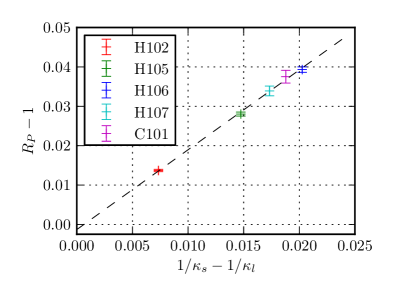
In Fig. 1 we demonstrate this for $J=P$, by showing $R_{P}(x,m_{s}-m_{\ell})-1$ at a fixed separation $x=(0,1,1,1)a$ and value of the lattice spacing $a\approx 0.085\,\textmd{fm}$ ($\beta=3.4$) as a function of $1/\kappa_{s}-1/\kappa_{\ell}$. This is carried out on different ensembles. As expected, the data lie on a straight line whose slope is proportional to $b_{P}$. The intercept is at the origin as there are no mass independent order $a$ effects in the current setting. The fact that a linear fit is consistent with this intercept demonstrates that the next-to-leading order lattice artefacts, that are proportional to $m^{2}a^{2}$, are small at our quark mass values. The point $x$ shown in this example appears to be well suited for the extraction of $b_{P}$. Below we will provide criteria to optimize this choice.

II.4 Observable for the $\tilde{b}_{J}$ coefficients

In contrast to the improvement coefficients $b_{J}$ accompanying non-singlet mass combinations, the $\tilde{b}_{J}$ coefficients can only be determined varying the average quark mass $\overline{m}$. Again, we start from the ratio of correlation functions Eq. (19), where this time $\rho\neq\sigma$ is necessary, i.e. information from at least two ensembles needs to be combined. The main set of CLS simulations Bruno:2014jqa is obtained along a trajectory of constant $\overline{m}$, where no sensitivity to $\tilde{b}_{J}$ exists. However, we have points on two additional mass plane trajectories at our disposal (for details, see Ref. Bali:2016umi ), one along which only the light quark mass is varied while the AWI strange quark mass is kept constant and one line, along which $\kappa_{\ell}=\kappa_{s}=\kappa^{(\rho)}$, i.e. $\overline{m}^{(\rho)}=m_{12}^{(\rho)}=m_{13}^{(\rho)}$. A coefficient $\tilde{b}_{J}$ can most easily be obtained along this “symmetric” trajectory, once $b_{J}$ is known, as in this case

$$\widetilde{R}_{J}(x,\overline{m}^{(\sigma)}-\overline{m}^{(\rho)}) \equiv\frac{G_{J^{(12)}}\left(n,a\overline{m}^{(\rho)},a\overline{m}^{(\rho)};g^{2}\right)}{G_{J^{(12)}}\left(n,a\overline{m}^{(\sigma)},a\overline{m}^{(\sigma)};g^{2}\right)}$$

$$=1+(2b_{J}+6\tilde{b}_{J})a\left(\overline{m}^{(\sigma)}-\overline{m}^{(\rho)}\right)$$

$$=1+\frac{1}{2}(b_{J}+3\tilde{b}_{J})\left(\frac{1}{\kappa^{(\sigma)}}-\frac{1}{\kappa^{(\rho)}}\right).$$ (21)

Note that again no knowledge of $\kappa_{\mathrm{crit}}$ is required. It is also possible to employ a pair of ensembles that differ in their $\kappa_{s}$ value but share a similar $\kappa_{\ell}$ value, eliminating the dependence on $b_{J}$ altogether when only light quark correlation functions are considered.

Figure 2: Dependence of the ratio $\widetilde{R}_{P}-1$ at the separation $x=(0,1,2,2)a$ as a function of the inverse hopping parameter difference $1/\kappa^{(\sigma)}-1/\kappa^{(\rho)}$.

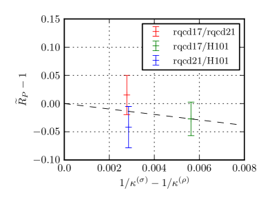
We demonstrate how $\tilde{b}_{P}$ can be extracted from the slope of $\widetilde{R}_{J}$ in Fig. 2: Using a set of three $m_{\ell}=m_{s}$ ensembles at $\beta=3.4$, we evaluate the ratio of correlators for all three possible pairs of ensembles. Note that the statistical errors are much larger than in the case of $b_{P}$, mostly because the numerator and denominator of Eq. (21) are uncorrelated.

III Behaviour at short and long distances

In this section we discuss corrections to the ratios $R_{J}(x,\Delta m)$ and $\widetilde{R}(x,\Delta\overline{m})$, see Eqs. (20) and (21), at large and short distances and define improved observables. We employ Euclidean spacetime conventions throughout.

III.1 Continuum expectation

The components of the propagator $S_{F}(x)\equiv S_{F}(x,0)$ for a quark $\psi^{i}_{\alpha}$ propagating from a four-position $0$ to $x$ are given as,

$$S_{F\alpha\beta}^{ij}(x)=\psi^{i}_{\alpha}(x)\overline{\psi}_{\beta}^{j}(0)=-\overline{\psi}_{\beta}^{j}(0)\psi^{i}_{\alpha}(x)\,,$$ (22)

where $\alpha,\beta$ denote spinor and $i,j$ colour indices. This receives perturbative and non-perturbative contributions. The massive free case propagator reads (see, e.g., Ref. Chu:1993cn ):

$$S_{F}(x) =\frac{1}{(2\pi)^{2}}\left[\gamma_{\mu}x_{\mu}\frac{m^{2}}{x^{2}}K_{2}(m|x|)+\frac{m^{2}}{|x|}K_{1}(m|x|)\right]$$

$$=\frac{1}{2\pi^{2}}\frac{\gamma_{\mu}x_{\mu}}{x^{4}}\left(1-\frac{m^{2}x^{2}}{4}\right)+\frac{m}{4\pi^{2}}\frac{1}{x^{2}}+\cdots,$$ (23)

where $K_{1}(z)$ and $K_{2}(z)$ are modified Bessel functions of the second kind. The leading non-perturbative contributions can be obtained, expanding

$$S_{F\alpha\beta}^{ij}(x)=-\overline{\psi}_{\beta}^{j}(0)\psi^{i}_{\alpha}(0)-x_{\mu}\overline{\psi}_{\beta}^{j}(0)[D_{\mu}\psi_{\alpha}]^{i}(0)+\cdots.$$ (24)

The colour, spinor and Lorentz structure then implies that

$$\langle\overline{\psi}_{\beta}^{j}\psi^{i}_{\alpha}\rangle =b\delta^{ij}\delta_{\alpha\beta}\,,$$ (25)

$$\langle\overline{\psi}_{\beta}^{j}[D_{\mu}\psi_{\alpha}]^{i}\rangle =c\delta^{ij}\left(\gamma_{\mu}\right)_{\alpha\beta},$$ (26)

where the constants $b$ and $c$ are easily determined:

$$\langle\overline{\psi}\psi\rangle =\sum_{i,\alpha}\langle\overline{\psi}_{\alpha}^{i}\psi_{\alpha}^{i}\rangle=4Nb\,,$$ (27)

$$m\langle\overline{\psi}\psi\rangle =-\gamma_{\mu}\langle\overline{\psi}D_{\mu}\psi\rangle$$

$$=-\sum_{i,\alpha,\beta,\mu}\left(\gamma_{\mu}\right)_{\alpha\beta}\langle\overline{\psi}_{\beta}^{i}[D_{\mu}\psi_{\alpha}]^{i}\rangle$$

$$=-cN\sum_{\mu}\mathrm{tr}\,\gamma_{\mu}\gamma_{\mu}=-16Nc\,.$$ (28)

Above we made use of the equations of motion and $N=3$ is the number of colours.

Collecting our results gives

$$S_{F}^{ij}(x) =f(x)\delta^{ij}\mathds{1}+g_{\mu}(x)\gamma_{\mu}\delta^{ij}+\cdots,$$ (29)

$$f(x) =\frac{m}{4\pi^{2}}\frac{1}{x^{2}}-\frac{1}{4N}\langle\overline{\psi}\psi\rangle\,,$$ (30)

$$g_{\mu}(x) =x_{\mu}\left[\frac{1}{2\pi^{2}x^{4}}-\frac{m^{2}}{8\pi^{2}x^{2}}+\frac{m}{16N}\langle\overline{\psi}\psi\rangle\right].$$ (31)

Note that some one-loop corrections to this expression can be found, e.g., in Ref. Gimenez:2005nt .

We are interested in correlation functions of the type

$$\left\langle J^{(12)}(x)\overline{J}^{(12)}(0)\right\rangle =\pm\left\langle[\overline{\psi}_{1}\Gamma\psi_{2}](x)[\overline{\psi}_{2}\Gamma\psi_{1}](0)\right\rangle$$

$$=\mp\left\langle\mathrm{tr}\,\left[\Gamma S_{F,2}(x)\Gamma\gamma_{5}S_{F,1}(x)\gamma_{5}\right]\right\rangle,$$ (32)

where $S_{F,j}$ is the propagator of a quark of flavour $j$ and we used the $\gamma_{5}$-Hermiticity $S_{F}^{\dagger}(0,x)=\gamma_{5}S_{F}(x,0)\gamma_{5}$. The upper signs refer to $J\in\{S,P,V\}$ and the lower signs to $J=A$. Note that as we restrict ourselves to non-singlet currents, the Wick contraction yields only one term.

It is now easy to see that

$$\left\langle J^{(12)}(x)\overline{J}^{(12)}(0)\right\rangle =\mp N\left[f_{1}(x)f_{2}(x)\mathrm{tr}\,(\Gamma^{2}\gamma_{5}^{2})\right.$$

$$\quad+\left.g_{1\mu}(x)g_{2\nu}(x)\mathrm{tr}\,\left(\Gamma\gamma_{\nu}\Gamma\gamma_{5}\gamma_{\mu}\gamma_{5}\right)\right]$$

$$=N\left[-4f_{1}(x)f_{2}(x)\right.$$

$$\quad\pm\left.g_{1\mu}(x)g_{2\nu}(x)\mathrm{tr}\,\left(\Gamma\gamma_{\nu}\Gamma\gamma_{\mu}\right)\right].$$ (33)

Evaluating the above traces for the combinations Eqs. (14)–(17) gives

$$G_{J^{(12)}}(x) =4N\left[-f_{1}(x)f_{2}(x)+s_{J}g_{1\mu}(x)g_{2\mu}(x)\right]\cdots$$

$$=\frac{N}{\pi^{4}}\frac{s_{J}}{x^{6}}-\frac{N}{4\pi^{4}}\frac{m_{1}m_{2}+s_{J}(m_{1}^{2}+m_{2}^{2})}{x^{4}}+$$

$$\quad+\frac{N}{16\pi^{4}}\frac{s_{J}m_{1}^{2}m_{2}^{2}}{x^{2}}$$

$$\quad+\frac{1}{8\pi^{2}}\frac{(2+s_{J})(m_{1}+m_{2})\langle\overline{\psi}\psi\rangle}{x^{2}}$$

$$\quad+\frac{1}{32\pi^{2}}\frac{s_{J}\langle FF\rangle}{x^{2}}+\cdots,$$ (34)

where

$$s_{S}=1\,, s_{P}=-1\,,$$ (35)

$$s_{V}=-\frac{1}{2}\,, s_{A}=\frac{1}{2}\,.$$ (36)

The contribution from the non-perturbative gluon condensate that we added to Eq. (34) is due to the possibility of a gluon coupling to each of the quark lines and can be inferred from the results of Refs. Reinders:1981sy ; Reinders:1984sr ; Jamin:1992se . Note that up to the overall sign convention and our prefactor $1/4$ in the definitions Eqs. (16) and (17) of $G_{V}$ and $G_{A}$, the above result is consistent with the equal mass expressions obtained in Ref. Tomii:2016xiv . Four-loop radiative corrections for the massless case can be found in Ref. Chetyrkin:2010dx .

Taking ratios of correlation functions obtained for different mass parameters gives

$$\frac{G_{J^{(12)}}(x)}{G_{J^{(34)}}(x)} =1+(A^{J}_{12}-A^{J}_{34})x^{2}$$

$$+\left[\left(A^{J}_{34}\right)^{2}-A^{J}_{12}A^{J}_{34}+B^{J}_{12}-B^{J}_{34}\right]x^{4}+\cdots,$$ (37)

with the mass dependent coefficients

$$A^{J}_{jk} =-\frac{1}{4}\left(m_{j}^{2}+m_{k}^{2}+\frac{m_{j}m_{k}}{s_{J}}\right)\,,$$ (38)

$$B^{J}_{jk} =\frac{\pi^{2}}{32N}\langle FF\rangle+\frac{m_{j}^{2}m_{k}^{2}}{16}$$

$$\quad+\frac{\pi^{2}}{8N}\frac{2+s_{J}}{s_{J}}(m_{j}+m_{k})\langle\overline{\psi}\psi\rangle\,.$$ (39)

We will make use of this expression where, in our regime of quark masses, the last term is the dominant one. The Gell-Mann–Oakes–Renner relation

$$(m_{j}+m_{k})\langle\overline{\psi}\psi\rangle=-F_{0}^{2}M_{jk}^{2}$$ (40)

can be used to substitute the chiral condensate term, thereby eliminating any free parameter. $M_{jk}$ above denotes the mass of a pseudoscalar meson composed of (anti)quarks of masses $m_{j}$ and $m_{k}$ and the pion decay constant in the $N_{f}=3$ chiral limit reads $F_{0}=86.5(1.2)\,\textmd{MeV}$ Aoki:2016frl ; Agashe:2014kda . Note that to order $x^{4}$ the gluon condensate does not contribute to the ratio Eq. (37) as it cancels from the difference $B^{J}_{12}-B^{J}_{34}$.

III.2 Lattice corrections

Now that we have worked out order $x^{2}$ and $x^{4}$ corrections, we will also investigate the short distance, order $a$ corrections to $b_{J}$.

The correlators can be computed in lattice perturbation theory in a volume of $N_{t}\times N^{3}$ sites. Unsurprisingly, we find the result at short distances to depend only weakly on the volume. Therefore, we employ antiperiodic fermionic boundary conditions in time, in spite of the fact that most of the analysed ensembles have open boundaries Luscher:2011kk ; Bruno:2014jqa . We start from the free Wilson quark propagator

$$S_{F}(x)=\frac{1}{(2\pi)^{4}}\sum_{p}\frac{-i\gamma_{\mu}\bar{p}_{\mu}+M(p)}{\sum_{\mu}\bar{p}_{\mu}^{2}+M^{2}(p)}\exp\left(ipx\right)\,,$$ (41)

where $\bar{p}_{\mu}=a^{-1}\sin(ap_{\mu})$, $p=(p_{0},p_{1},p_{2},p_{3})$ with

$$p_{0} =-\frac{\pi}{a}+\frac{\pi}{N_{t}a},-\frac{\pi}{a}+\frac{3\pi}{N_{t}a},\ldots,\frac{\pi}{a}-\frac{\pi}{N_{t}a},$$

$$p_{i} =-\frac{\pi}{a}+\frac{2\pi}{Na},\ldots,\frac{\pi}{a}\,,$$ (42)

and

$$M(p)=m_{0}+\frac{2}{a}\sum_{\mu}\sin^{2}\left(\frac{ap_{\mu}}{2}\right)\,.$$ (43)

Using a simple computer program, we can evaluate and combine two of these quark propagators into a correlator $G_{J}(x)$. This then enables us to obtain (mass dependent) tree-level results for the ratios $R_{J}$ and $\widetilde{R}_{J}$, see Eqs. (20) and (21). We label these ratios as $R_{J}^{\mathrm{tree}}$ and $\widetilde{R}_{J}^{\mathrm{tree}}$.

Subtracting the tree-level expectation from the lattice data will not only reduce lattice artefacts but also the leading factor of $1$ cancels identically from Eqs. (20) and (21). Moreover, the impact of the mass dependent perturbative $A^{J}_{jk}$ coefficients and of the $m_{j}^{2}m_{k}^{2}$ term within $B^{J}_{jk}$ (see Eqs. (38) and (39)) on Eq. (37) is removed to leading order. The effect of these terms was tiny in any case in comparison to that of the chiral condensate appearing within $B^{J}_{jk}$: $m\ll|\langle\overline{\psi}\psi\rangle|^{1/3}$. Indeed, after subtracting the leading order perturbative expectation we are unable to resolve any remaining $x^{2}$ term within our numerical precision.

Figure 3: Tree-level improvement coefficients. The data correspond to the largest mass difference that we can encounter. The band indicates the region with cut-off effects smaller than 15%. All separations $n=x/a$ within this band are accepted.

III.3 Improved observables and the choice of the Euclidean distance

Using the tree-level lattice perturbation theory results of Sec. III.2 above as well as Eqs. (37), (39) and (40), we define the improved ratio of correlators, cf. Eq. (20):

$$B_{J}(x,m_{s}-m_{\ell}) \equiv 1+\biggl{[}R_{J}(x,m_{s}-m_{\ell})-R^{\mathrm{tree}}_{J}(x,m_{s}-m_{\ell})\left.+\frac{\pi^{2}}{8N}\frac{2+s_{J}}{s_{J}}\left(M_{\pi}^{2}-M_{K}^{2}\right)F_{0}^{2}x^{4}\right]\times\left(\frac{1}{\kappa_{s}}-\frac{1}{\kappa_{\ell}}\right)^{-1}$$

$$=b_{J}+\mathcal{O}(x^{6})+\mathcal{O}(g^{2}a)+\mathcal{O}(g^{2}a^{2}/x^{2})+\cdots\,,$$ (44)

where we have neglected small mass dependent terms of $\mathcal{O}(g^{2}x^{2})$ and $\mathcal{O}(g^{2}x^{4})$. $M_{K}=M_{13}$ and $M_{\pi}=M_{12}$ are the kaon and pion masses, most of which are published in Refs. Bali:2016umi ; Bruno:2014jqa . We also define $\widetilde{B}_{J}$, analogously generalizing Eq. (21):

$$\widetilde{B}_{J}(x,\overline{m}^{(\sigma)}-\overline{m}^{(\rho)}) \equiv 1+\biggl{[}\widetilde{R}_{J}(x,\overline{m}^{(\sigma)}-\overline{m}^{(\rho)})-\widetilde{R}^{\mathrm{tree}}_{J}(x,\overline{m}^{(\sigma)}-\overline{m}^{(\rho)})\left.+\frac{\pi^{2}}{8N}\frac{2+s_{J}}{s_{J}}\left({M_{\pi}^{(\rho)}}^{2}-{M_{\pi}^{(\sigma)}}^{2}\right)F_{0}^{2}x^{4}\right]$$

$$\qquad\times\left(\frac{1}{\kappa^{(\sigma)}}-\frac{1}{\kappa^{(\rho)}}\right)^{-1}=b_{J}+3\tilde{b}_{J}+\mathcal{O}(x^{6})+\mathcal{O}(g^{2}a)+\mathcal{O}(g^{2}a^{2}/x^{2})+\cdots\,.$$ (45)

Before implementing the above equations, we must decide on the $x=na$ distances to be considered. Differences between improvement coefficients determined for different choices of $x$ will be of order $a$, as long as $x^{2}\ll 1/\Lambda^{2}$. In the end we will select one and the same lattice direction $N_{0}$ to define our improvement condition at $x_{0}\propto N_{0}a$. Ideally, for this choice order $a$ corrections to $b_{J}$ and to $\tilde{b}_{J}$ should be as small as possible. As can be seen from the last term of Eqs. (44) and (45), $B_{J}$ and $\widetilde{B}_{J}$ need to be determined at a fixed physical distance $|x|=|x_{0}|$. On a discrete lattice $x_{0}$ cannot be kept fixed when changing the spacing, however, we will use the $n_{0}\propto N_{0}$ value that is closest to our choice of $x_{0}\approx n_{0}a$. In addition to this reference point $n_{0}$, we realize additional vectors $n$ to enable an estimation of the size of $x^{6}$ and higher order continuum effects that have not been accounted for.

Table 1: Set of points selected for the non-perturbative analysis. We average over equivalent directions in terms of the spatial cubic symmetry including inversions and time reflections. The point $N_{0}$ appears in boldface.

Channel	$(n_{0}n_{1}n_{2}n_{3})$
$S$	$(0001)$, $(0011)$, $(0012)$, $(0112)$, $(0113)$, ${\bf(0122)}$, $(0222)$, $(1000)$, $(1001)$, $(1002)$, $(1012)$, $(1013)$, $(1022)$, $(1123)$, $(1133)$, $(1223)$, $(1233)$, $(2001)$, $(2011)$, $(2012)$, $(2022)$, $(2113)$, $(2123)$, $(2133)$, $(2222)$, $(2223)$, $(2233)$, $(3011)$, $(3112)$, $(3113)$, $(3122)$, $(3123)$, $(3222)$
$P$	$(0111)$, $(0112)$, $(0113)$, ${\bf(0122)}$, $(0123)$, $(0133)$, $(0222)$, $(0223)$, $(0233)$, $(0333)$, $(1011)$, $(1012)$, $(1013)$, $(1022)$, $(1023)$, $(1033)$, $(2011)$, $(2012)$, $(2013)$, $(2022)$, $(2023)$, $(2033)$, $(3003)$, $(3011)$, $(3012)$, $(3013)$, $(3022)$, $(3023)$
$V$	$(0112)$, $(0113)$, ${\bf(0122)}$, $(0123)$, $(0133)$, $(0222)$, $(0223)$, $(0233)$, $(0333)$, $(1012)$, $(1013)$, $(1022)$, $(1023)$, $(1033)$, $(2011)$, $(2012)$, $(2013)$, $(2022)$, $(2023)$, $(2033)$, $(3011)$, $(3012)$, $(3013)$, $(3022)$, $(3023)$, $(3033)$
$A$	$(0011)$, $(0112)$, ${\bf(0122)}$, $(1001)$, $(1012)$, $(1022)$, $(1133)$, $(1233)$, $(2011)$, $(2012)$, $(2133)$, $(2233)$, $(3113)$, $(3123)$, $(3223)$

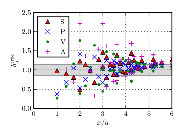
As a first step we define a subset of vectors for which tree-level cut-off effects are small. In Fig. 3 we show improvement coefficients $b_{J}^{\textrm{tree}}$ evaluated in tree-level lattice perturbation theory. For this comparison we set $m_{\ell}=0$ and $m_{s}$ equal to the strange quark AWI mass obtained on the ensemble H106, see Ref. Bali:2016umi . This mass approximately corresponds to the physical strange quark mass, obtained on the coarsest lattice spacing in use. This choice represents the largest $a(m_{s}-m_{\ell})$ difference that we can encounter. Note that in tree-level perturbation theory the AWI and lattice quark masses coincide. The higher order differences will be addressed in the discussion of systematic errors, see Sec. IV.2. For the subsequent analysis we select only those vectors $n$ for which the deviation of $b_{J}^{\textrm{tree}}$ from the continuum expectation $b_{J}=1$ is smaller than 15%.

Table 1 summarizes the accepted lattice vectors for the different currents. One separation that is common to all the investigated channels is $N_{0}=(0,1,2,2)$. For our present range of lattice spacings, see Table 2, this means $0.26\,\textmd{fm}>|N_{0}|a\geq 0.15\,\textmd{fm}$. We wish to keep $|x_{0}|$ as small as possible to minimize the systematics. A suitable compromise in view of the analysed lattice spacings is $|x_{0}|=0.2\,\textmd{fm}$. Then, within this range $n_{0}=N_{0}$. For $a<0.045\,\textmd{fm}$, which is the case for a set of newly generated CLS ensembles at $\beta=3.85$, we will have to increase $n_{0}=2N_{0}$ and for $a<0.027\,\textmd{fm}$ $n_{0}=3N_{0}$ to keep $|n_{0}|a\approx|x_{0}|$. Within the range of lattice spacings that we cover here $|x_{0}|$ varies by $\pm 25\%$ around the target value and one may wonder about any associated systematics. We investigate this in the Appendix.

We use the vector $n_{0}=N_{0}$ (and all its 24 equivalent permutations of spatial components and signs) to compute the improvement coefficients. All the remaining vectors within the range $0.15\,\textmd{fm}\lesssim|n|a\lesssim 0.4\,\textmd{fm}$ are used to estimate systematic errors.

IV Estimation of systematic errors

IV.1 Finite volume effects

The improvement coefficients describe short distance effects and therefore should be insensitive to the simulated volume. However, $b_{J}$ and $\tilde{b}_{J}$ obtained using Eqs. (44) and (45) will inherit the dependence of the correlation functions $G_{J}$, that enter $R_{J}$ and $\widetilde{R}_{J}$, on $L=Na$. For sufficiently small separations $|x|\ll L$ this dependence should become negligible. Indeed, in a quenched setup finite volume effects on ratios of massless correlators evaluated at separations $|x|/L<1/8$ were found to be below 1% Cichy:2016qpu . Extrapolating tree-level finite volume lattice perturbation theory results to the continuum limit, keeping $|x|/L=|n|/N$ and $mx$ fixed, and comparing the outcome to infinite volume continuum perturbation theory, we confirmed that this statement remains valid also for the ratio $R_{J}$ of Eq. (20): For $|x|/L<1/8$ the differences are negligible, compared to the other systematic errors that we will account for below. We remark that all CLS ensembles satisfy the condition $LM_{\pi}\gtrsim 4$, and hence the inequality $L>8|x_{0}|=1.6\,\textmd{fm}$ always holds. The worst case that we encounter corresponds to our coarse “H” ensembles where $|n_{0}|a\approx|x_{0}|$ takes its largest value in physical units and $L/|n_{0}|a=32/3$. Also note that in a non-perturbative setting finite size effects will be even smaller, due to the mass gap.

(a) Scalar

(b) Pseudoscalar

(c) Vector

(d) Axial

Figure 4: $B_{J}(x)$ for the ensembles H102, S400 and N203 which share similar pion and kaon masses, see Table 2. Solid lines denote the $x^{6}$ fit, Eq. (46), to the data in the shaded region. The $n_{0}a\approx x_{0}$ points that are used to define the $b_{J}$ coefficients are plotted as large circles. The difference between a fit function at this position from its value at $x=0$ constitutes one of our systematic errors.

IV.2 Perturbative and non-perturbative corrections

Different conditions can be used to define the improvement coefficients. As long as these definitions differ by order $a$ terms all such schemes are equivalent in the sense that improved expectation values of physical observables will extrapolate to one and the same continuum limit, linear in $a^{2}$, with $g^{2}a^{2}$, $a^{3}$ and higher order corrections. For instance, we could have selected a different value of $|x_{0}|$ along a different direction $N_{0}$: Order $a$ corrections to the $b_{J}$ and $\tilde{b}_{J}$ coefficients do not constitute a source of systematics but correspond to a particular convention.

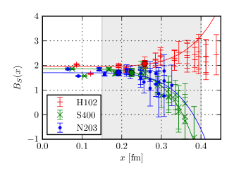
In Eqs. (44) and (45) we defined the observables $B_{J}(x,m_{s}-m_{\ell})$ and $\widetilde{B}_{J}(x,\overline{m}^{(\rho)}-\overline{m}^{(\sigma)})$, where the leading non-perturbative contribution (proportional to the quark condensate) is subtracted and also the continuum perturbative mass dependence is cancelled at tree-level. Higher order mass dependent perturbative terms are neglected and we employed AWI rather than renormalized quark masses, which will also differ from each other at higher orders. For all lattice spacings and quark mass combinations investigated, at $n_{0}a\approx x_{0}$ we find these mass dependent tree-level corrections to contribute only at the per mille level to $B_{J}$ and $\widetilde{B}_{J}$. Therefore, errors from neglecting the associated radiative corrections will be completely insignificant in comparison to our statistical errors. However, we also corrected for the leading non-perturbative effect that is proportional to $x^{4}$. This correction relies not only on the validity of the Gell-Mann–Oakes–Renner relation in our regime of quark masses but there exist also perturbative corrections to the Wilson coefficient, that we have neglected. Figure 4 demonstrates that, with the exception of the pseudoscalar channel and up the scattering at short distances between different lattice points, $B_{J}$ is almost perfectly flat up to distances $|x|\approx 0.25\,\textmd{fm}$, indicating that such corrections are small at $|x_{0}|=0.2\,\textmd{fm}$. We add 20% of the subtracted $x^{4}$ terms to our systematic error budget to reflect this uncertainty. In order to discriminate whether the effect seen in the pseudoscalar channel is due to particularly large radiative corrections, lattice artefacts or interference from different higher order terms, a perturbative calculation of the $x^{4}$ Wilson coefficient is ongoing.

After adding the uncertainty of the $x^{4}$ subtraction to our error budget, any remaining correction should be proportional to $x^{6}$ and higher orders. To account for this we fit

$$B_{J}(x)=\alpha_{J}+\beta_{J}x^{6}$$ (46)

for each quark mass combination and current within the window $0.15\,\textmd{fm}\lesssim|x|\lesssim 0.4\,\textmd{fm}$. A subset of these fits is shown in Fig. 4. We quote $|\beta_{J}(n_{0}a)^{6}|$ as a second systematic error. Note that these fits are only performed to estimate the systematics and the curves shown do not adequately represent the data, in particular at short distances where lattice artefacts are visible and statistical errors are small.

Table 2: Summary of CLS (and RQCD) ensembles used in this study. “O” stands for open and “P” for periodic boundary conditions (BC) in time. $N_{\mathrm{conf}}$ denotes the number of analysed configurations and “sep.” is the separations between two successive measurements in molecular dynamics units.

$\beta$	$a/\textmd{fm}$	Ensemble	BC	$N_{t}$	$N$	$\kappa_{\ell}$	$\kappa_{s}$	$M_{\pi}$	$M_{K}$	$N_{\mathrm{conf}}$	sep.
3.4	0.085	H101	O	96	32	0.136759	0.136759	422	422	100	40
3.4	0.085	H102	O	96	32	0.136865	0.136549339	356	442	100	40
3.4	0.085	H105	O	96	32	0.136970	0.13634079	282	567	103	20
3.4	0.085	H106	O	96	32	0.137016	0.136148704	272	519	57	20
3.4	0.085	H107	O	96	32	0.136946	0.136203165	368	549	49	20
3.4	0.085	C101	O	96	48	0.137030	0.136222041	223	476	59	40
3.4	0.085	C102	O	96	48	0.137051	0.136129063	223	504	48	40
3.4	0.085	rqcd017	P	32	32	0.1368650	0.1368650	238	238	150	20
3.4	0.085	rqcd021	P	32	32	0.136813	0.136813	340	340	50	20
3.46	0.076	S400	O	128	32	0.136984	0.136702387	354	446	83	40
3.55	0.064	N203	O	128	48	0.137080	0.136840284	345	441	74	40
3.7	0.050	J303	O	192	64	0.137123	0.1367546608	260	478	38	40

(a) Scalar

(b) Pseudoscalar

(c) Vector

(d) Axial

Figure 5: Numerical results for $b_{J}$ for all the mass non-degenerate ensembles. The outer (blue) error bars denote the total uncertainties while the inner (red) error bars indicate the statistical errors.

Table 3: Numerical results for the $b_{J}$ improvement coefficients. The first error is statistical, the second error corresponds to a 20% uncertainty of the Wilson coefficient of the non-perturbative $x^{4}$ correction and the third error is an estimate of the size of order $x^{6}$ corrections, see Sec. IV.2.

$\beta$	Ensemble	$b_{S}$	$b_{P}$	$b_{V}$	$b_{A}$
3.4	H102	2.12(14)(5)(1)	2.46(20)(2)(28)	1.38(3)(5)(5)	1.71(7)(8)(2)
	H105	1.72(18)(5)(22)	2.85(19)(2)(50)	1.45(4)(5)(5)	1.75(7)(8)(3)
	H106	2.01(16)(5)(5)	2.73(12)(2)(33)	1.45(4)(5)(7)	1.89(6)(9)(3)
	H107	2.06(16)(5)(1)	2.54(4)(2)(10)	1.38(5)(5)(7)	1.82(7)(8)(5)
	C101	2.26(23)(5)(1)	2.78(13)(2)(29)	1.50(4)(5)(6)	1.90(14)(8)(3)
	C102	2.11(6)(5)(3)	2.64(15)(2)(29)	1.57(4)(5)(7)	1.76(8)(8)(3)
3.46	S400	1.62(22)(7)(11)	2.54(24)(2)(23)	1.46(4)(7)(8)	1.49(15)(12)(6)
3.55	N203	1.67(9)(5)(2)	1.98(7)(2)(11)	1.40(3)(5)(5)	1.38(6)(9)(5)
3.7	J303	1.56(6)(4)(1)	1.63(4)(1)(5)	1.40(2)(4)(4)	1.26(5)(7)(5)

Table 4: Fit parameters for the parametrizations of $b_{J}(g^{2})$ Eqs. (47) and (48) with the one-loop coefficients of Ref. Taniguchi:1998pf . We also include parametrizations for $\mathcal{A}=b_{P}-b_{A}+b_{S}$ and $b_{A}-b_{P}$. Note that the leading order result for the latter combination reads 0, instead of 1.

Coefficient	$b_{J}^{\text{one-loop}}$	$\gamma_{J}$	$\delta_{J}$	cov($\gamma_{J}$,$\delta_{J}$)
$b_{S}$	0.1526	$-0.439(50)$	$-0.535(14)$	0.972
$b_{P}$	0.1187	$-0.354(54)$	$-0.540(11)$	0.945
$b_{V}$	0.1181	$0.596(206)$	—	—
$b_{A}$	0.1175	$-0.523(33)$	$-0.554(10)$	0.984
$\mathcal{A}$	0.1538	$-0.252(145)$	$-0.522(26)$	0.973
$b_{A}-b_{P}$	$-0.0012$	$22.6(20.7)$	$-0.512(62)$	0.968

V Results

We introduce the ensembles and analysis methods used, before we present results on the $b_{J}$ coefficients, including an interpolating parametrization, that is based on one-loop perturbative results. For convenience we also include two combinations of improvement coefficients that are frequently needed. Subsequently, we determine the $\tilde{b}_{J}$ coefficients at our coarsest lattice spacing ($a\approx 0.085\,\textmd{fm}$, $\beta=3.4$) as a proof of concept.

V.1 Overview of the used ensembles

We use ensembles generated within the CLS initiative. In Table 2 we summarize the ensembles employed and how many measurements were taken; for more details see Refs. Bruno:2014jqa ; Bali:2016umi . Typically we perform 50 to 100 measurements, that are separated by 20 to 40 molecular dynamics units (MDUs) in the Markov Monte-Carlo chain. The largest integrated autocorrelation time is associated with the Wilson flow observable $E(t_{0})$, which does not exceed $\approx 100$ MDU, even at $\beta=3.7$ Bruno:2014jqa . Indeed, binning our data gives no indication of autocorrelations. The statistical errors are computed with the jackknife method.

V.2 Results for $b_{J}$

(a) Scalar

(b) Pseudoscalar

(c) Vector

(d) Axial

Figure 6: $b_{J}$ as functions of $g^{2}$. The error bands correspond to Eqs. (47)–(48) with the parameter values of Table 4. The dashed lines are the perturbative one-loop expectations.

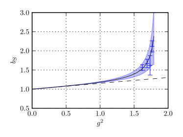
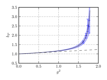
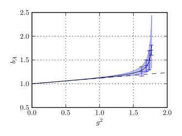
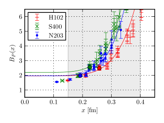
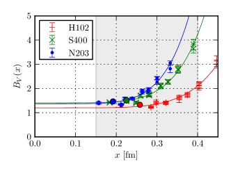
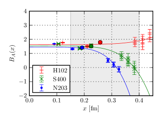
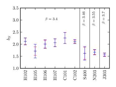
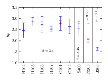
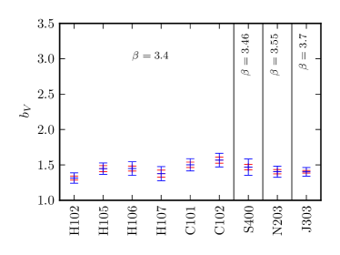
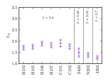
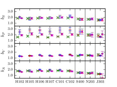
In Table 3 we list our results for each ensemble. These are also visualized in Fig. 5. Note that at $\beta=3.4$ we have several mass combinations at our disposal, giving several independent results that turn out to be compatible with each other within errors. We will quote the H102 results as our reference values since the pion and kaon masses are similar in this case to those of S400 and N203. Statistical and systematic errors depend on the lattice spacing and quark mass combinations used and vary considerably between the ensembles. Most of the results in the pseudoscalar channel are dominated by the systematic uncertainties. However, the systematic errors decrease as we approach finer lattices. Note that the $b_{J}$ coefficients from the ensemble with the finest lattice spacing, J303, have combined errors ranging from 4.8% to 7.7%, whereas the relative uncertainty on $b_{P}$ determined on H102 amounts to 14%.

We parameterize the $g^{2}=6/\beta$ dependence of our results using a two parameter rational approximation:

$$b_{J}(g^{2}) =1+b_{J}^{\textrm{one-loop}}g^{2}\frac{1+\gamma_{J}g^{2}}{1+\delta_{J}g^{2}}\quad\text{for}\quad J=S,P,A\,,$$ (47)

$$b_{J}(g^{2}) =1+b_{J}^{\textrm{one-loop}}g^{2}(1+\gamma_{J}g^{2})\quad\text{for}\quad J=V\,.$$ (48)

Note that $b_{V}$ is well described by a one parameter fit, such that in this case allowing for $\delta_{V}\neq 0$ does not result in a stable fit. The parameters

$$b_{P}^{\textrm{one-loop}} =0.0890(1)C_{F}\,, b_{S}^{\textrm{one-loop}}=0.11444(1)C_{F}\,,$$ (49)

$$b_{A}^{\textrm{one-loop}} =0.0881(1)C_{F}\,, b_{V}^{\textrm{one-loop}}=0.0886(2)C_{F}\,,$$ (50)

where $C_{F}=4/3$, correspond to the one-loop coefficients that were computed for our action in Ref. Taniguchi:1998pf , so that the parametrizations respect the known perturbative limits.

We include the ensembles H102, S400, N203 and J303 into our fit. Note that H102, S400 and N203 share similar pion and kaon masses. We combine the statistical and systematic uncertainties in quadrature. The fits are shown in Fig. 6 and the fit parameter values are collected in Table 4. The parameter values for the two parameter fits are highly correlated and we give the correlation coefficients in the last column of the table. This, along with the statistical errors of $\gamma_{J}$ and $\delta_{J}$, is used to generate the error bands shown in the figure. In the case of $\gamma_{V}$, where we carried out a one parameter fit, we obtained a value $\chi^{2}/3=0.29$ and rescaled the error on the fit parameter (and the error band shown) by $\sqrt{1/0.29}$ to be on the safe side. We remark that for our action no simulations are planned for $g^{2}$ values outside the bands shown, i.e. for $g^{2}>1.8$, where the above rational parametrizations exhibit poles.

One often encounters specific linear combinations of improvement coefficients. In Refs. Bhattacharya:2005rb and Bali:2016umi the coefficient

$$\mathcal{A}=b_{P}-b_{A}+b_{S}=b_{P}-b_{A}-2b_{m}$$ (51)

plays an important role while the combination $b_{A}-b_{P}$ is needed to convert AWI into renormalized quark masses. Therefore, we specifically analyse these combinations too and include the corresponding rational parametrizations in the last two lines of Table 4. Note that the small value of $b^{\text{one-loop}}_{A-P}=-0.0012$ for the combination $b_{A}-b_{P}$ results in a large $\gamma_{A-P}$ coefficient. This also means that for the parametrization to be accurate, in this case it is important to set $b^{\text{one-loop}}_{A-P}$ exactly to this value, ignoring its uncertainty of approximately $2\cdot 10^{-4}$.

V.3 Results for $\tilde{b}_{J}$

The $\tilde{b}_{J}$ improvement coefficients carry much larger statistical errors than their $b_{J}$ counterparts since one needs to combine data from at least two independent ensembles. Therefore, the errors cannot benefit from correlations between statistical fluctuations but always add up.

First, we compute $\widetilde{B}_{J}$ for pairs of the three symmetric line ensembles rqcd021, rqcd017 and H101 and find consistent results. Next, in order to combine information from all three ensembles, we correct the individual $\widetilde{R}_{J}$ ratios defined in Eq. (21) in the way suggested by Eq. (45) and extract the combination $b_{J}+3\tilde{b}_{J}$ from the linear slope of the $1/\kappa$ dependence at $n_{0}a\approx x_{0}$. Following the procedure outlined in Sec. IV.2, we then allow for 20% of the $x^{4}$ correction term as one systematic error and add another error, associated to the $x^{6}$ term from a fit according to Eq. (46). Finally, we subtract the $b_{J}$ values obtained on ensemble H102, see Table 3, to arrive at the results

$$\tilde{b}_{S} =\ \ 0.9\ (5.4)\ (0.1)\ (0.9)\,,$$ (52)

$$\tilde{b}_{P} =-6.8\ (4.5)\ (0.1)\ (0.2)\,,$$ (53)

$$\tilde{b}_{V} =-3.5\ (2.8)\ (0.1)\ (0.4)\,,$$ (54)

$$\tilde{b}_{A} =\ \ 0.5\ (3.4)\ (0.2)\ (0.3)\,,$$ (55)

where the first errors are statistical and the other two uncertainties correspond to the systematic errors explained above. Within large statistical errors, that dominate the error budget, all values are consistent with zero.

VI Conclusions and outlook

We computed “$b_{J}$” improvement coefficients parameterizing the linear cut-off effects that are proportional to non-singlet quark mass combinations for flavour non-singlet quark bilinear currents on a set of CLS ensembles at four lattice spacings: $a\approx 0.085\,\textmd{fm}$, $a\approx 0.076\,\textmd{fm}$, $a\approx 0.064\,\textmd{fm}$ and $a\approx 0.05\,\textmd{fm}$. We also provide first estimates of the $\tilde{b}_{J}$ coefficients that accompany the trace of the quark mass matrix.

Our method is based on the short distance behaviour of current-current correlation functions and turned out to be statistically very precise, given the relatively small computational effort. We benefited from subtracting the dominant non-perturbative effects as well as the leading perturbative lattice artefacts. We carefully investigated systematic errors related to non-perturbative and perturbative corrections as well as finite volume effects and included the relevant uncertainties into the errors of the results that we quote.

Our main result is the parametrization of the $b_{J}$ coefficients Eqs. (47) and (48) with the parameter values given in Table 4, which is valid for the range $3.4\leq\beta\leq 3.7$. In the future we will extend this range towards higher $\beta$ values and also increase the statistical precision. These coefficients become very important for heavy quark masses like that of the charm; for instance $b_{A}$ significantly contributes to charmed pseudoscalar meson decay constants. Neither can their effect be neglected if one is interested in matrix elements involving strange quarks within a (sub) percent level accuracy.

Preliminary results at our coarsest lattice spacing were obtained for the $\tilde{b}_{J}$ parameters too, see Eqs. (52)–(55). In this case we had to combine data from different gauge ensembles and could not benefit from cancellations of statistical fluctuations. This means that more measurements are required. Since the $\tilde{b}_{J}$ originate from sea quark effects, these are of order $g^{4}$ in perturbation theory. However, within our present uncertainties we cannot exclude large values of these coefficients, and our preliminary results in fact suggest that some of them may be unusually large.

It is known that the ratio of the singlet over the non-singlet mass renormalization constant $r_{m}$ is about $2.6$ at $\beta=3.4$ and still $1.5$ at $\beta=3.55$ Bali:2016umi , far from the asymptotic value of one. As a consequence of this decrease of $r_{m}$ with $\beta$, starting from a relatively high value, the combination $(2m_{\ell}+m_{s})a=(2/\kappa_{\ell}+1/\kappa_{s}-3/\kappa_{\mathrm{crit}})/2$ stays fairly constant within the range of investigated lattice spacings at fixed renormalized quark mass values, while naively one would have expected it to decrease with $a$. The sea always contains the relatively heavy strange quark, so that at realistic values of the sea quark masses the above combination (that accompanies $\tilde{b}_{J}$) is about 0.012 and 0.014 Bali:2016umi at $\beta=3.4$ and $\beta=3.55$, respectively. Therefore, a value $\tilde{b}_{A}=1$ would increase light pseudoscalar decay constants by more than 1%. Clearly, this needs to be investigated further, including $\beta>3.4$ and significantly increasing statistics, to enable a full order $a$ improved continuum limit to be taken for a wide range of physical observables. We also plan to extend the present study to different currents, including flavour-singlet operators.

Appendix A Impact of the quantization of lattice distances

The distance $|x_{0}|$ used to determine the improvement coefficients can in principle be chosen at will as long as $|x_{0}|=|n_{0}|a$ is kept (approximately) constant, to achieve the complete removal of order $a$ terms from continuum limit extrapolations of physical observables. We restricted ourselves to points where lattice artefacts on the $b_{J}$ coefficients are small — at least at tree-level. Keeping $|n_{0}|$ constant (rather than $|x_{0}|$) would result in corrections to the $b_{J}$ coefficients of order $1/|n_{0}|^{2}$ (rather than of order $a^{2}/x_{0}^{2}$), which will not vanish as the continuum limit is taken. We rely on non-perturbative corrections to be small in the continuum theory, which means $|x_{0}|\lesssim 0.25\,\textmd{fm}$ is a necessary condition for the method to be applicable. On the coarsest lattices of interest this translates into $|x_{0}|\lesssim 3a$. Clearly, at such separations the quantization of lattice distances cannot be neglected and indeed the data points shown in Fig. 4 at very short distances are not well described by continuous curves.

In this article we decided to take $n_{0}=mN_{0}$ along a fixed lattice direction $N_{0}=(0,1,2,2)$, which corresponds to the smallest distance appearing within all four channels shown in Table 1. We then set the multiple $m\in\mathbb{N}$ such that $m|N_{0}|a$ was closest to $|x_{0}|=0.2\,\textmd{fm}$. In our case this meant $m=1$ for all four lattice spacings, and we investigate the systematics of this approximation in this Appendix.

Table 5: The lattice points of Table 1 that are closest to $|x_{0}|=0.2\,\textmd{fm}$ from below ($x_{0<}$) and from above ($x_{0>}$) for the channels $J\in\{S,P,V,A\}$. In the case of $\beta=3.4$ the point $x_{0<}$ does not exist for $J=A$. Whenever $x_{0<}=N_{0}a$ or $x_{0>}=N_{0}a$ this is indicated using boldface.

$J$	$\beta$	$x_{0<}/a$	$x_{0>}/a$	$|x_{0<}|/\textmd{fm}$	$|x_{0>}|/\textmd{fm}$
	$3.4$	$(0012)$	$(0112)$	0.191	0.209
$S$	$3.46$	$(0112)$	${\bf(0122)}$	0.186	0.228
	$3.55$	${\bf(0122)}$	$(0113)$	0.193	0.214
	$3.7$	$(1123)$	$(1223)$	0.194	0.212
	$3.4$	$(0111)$	$(0112)$	0.148	0.209
$P$	$3.46$	$(0112)$	${\bf(0122)}$	0.186	0.228
	$3.55$	${\bf(0122)}$	$(0113)$	0.193	0.214
	$3.7$	$(0123)$	$(0223)$	0.187	0.206
	$3.4$	—	$(0112)$	—	0.209
$V$	$3.46$	$(0112)$	${\bf(0122)}$	0.186	0.228
	$3.55$	${\bf(0122)}$	$(0113)$	0.193	0.214
	$3.7$	$(0123)$	$(0223)$	0.187	0.206
	$3.4$	$(0011)$	$(0112)$	0.121	0.209
$A$	$3.46$	$(0112)$	${\bf(0122)}$	0.186	0.228
	$3.55$	${\bf(0122)}$	$(0113)$	0.193	0.214
	$3.7$	${\bf(0122)}$	$(1133)$	0.150	0.224

Figure 7: The improvement coefficients $b_{J}$, extracted for different choices of $x_{0}$. In addition to $x_{0}=N_{0}a$ (blue central point within each group of three points), the results obtained for $x_{0<}$ (left points where available) and $x_{0>}$ (right points) are shown, see Table 5. Inner error bars are statistical only. Outer error bars include systematics. The “H” and “C” ensembles correspond to $\beta=3.4$ ($a\approx 0.085\,\textmd{fm}$), S400 to $\beta=3.46$, N203 to $\beta=3.55$ and J303 to $\beta=3.7$ ($a\approx 0.050\,\textmd{fm}$).

In Table 5 we list for our four currents and four $\beta$ values the lattice distances $|x_{0<}|$ and $|x_{0>}|$ that are closest to $|x_{0}|=0.2\,\textmd{fm}$ from below and from above, within the set of points of small tree-level artefacts listed in Table 1. This is to be compared to the $|n_{0}|a=|N_{0}|a$ values of $0.256\,\textmd{fm}$, $0.228\,\textmd{fm}$, $0.193\,\textmd{fm}$ and $0.150\,\textmd{fm}$ at $\beta=3.4$, $3.46$, $3.55$ and $3.7$, respectively. We could have relaxed the restriction to one lattice direction $N_{0}$ and for instance have used the $|x_{0<}|$ or $|x_{0>}|$ values (or an average of these) to define the improvement coefficients. In Fig. 7 we compare the results of such different strategies. For each group of three points the central point corresponds to the result obtained using $N_{0}a$ with the point on the left corresponding to $x_{0<}$ and to the right to $x_{0>}$. For the vector channel at $\beta=3.4$ no $x_{0<}$ point exists and in some cases either $x_{0<}$ or $x_{0>}$ happen to coincide with $N_{0}a$, see Table 5. At $\beta=3.7$ even $|x_{0<}|$ is larger than $|N_{0}|a$. Within present errors the different results mostly appear to be consistent. The deviation of $|N_{0}|a$ from $x_{0}=0.2\,\textmd{fm}$ is largest at $\beta=3.4$ and $\beta=3.7$ and at $\beta=3.4$ there appears to be some tension in the pseudoscalar channel. This will be addressed with increased precision in the near future.

References

- (1) Martin Lüscher, Stefan Sint, Rainer Sommer, and Peter Weisz, “Chiral symmetry and improvement in Lattice QCD,” Nucl. Phys. B 478, 365 (1996), arXiv:hep-lat/9605038 [hep-lat]
- (2) Martin Lüscher, Stefan Sint, Rainer Sommer, Peter Weisz, and Ulli Wolff (ALPHA Collaboration), “Nonperturbative improvement of Lattice QCD,” Nucl. Phys. B 491, 323 (1997), arXiv:hep-lat/9609035 [hep-lat]
- (3) Kurt Symanzik, “Continuum limit and improved action in lattice theories. 1. Principles and theory,” Nucl. Phys. B 226, 187 (1983)
- (4) Mattia Bruno et al. (CLS), “Simulation of QCD with flavors of non-perturbatively improved Wilson Fermions,” J. High Energy Phys. 02, 043 (2015), arXiv:1411.3982 [hep-lat]
- (5) Bijan Sheikholeslami and R. Wohlert, “Improved continuum limit lattice action for QCD with Wilson Fermions,” Nucl. Phys. B 259, 572 (1985)
- (6) Peter Weisz, “Continuum limit improved lattice action for pure Yang-Mills theory. 1..” Nucl. Phys. B 212, 1 (1983)
- (7) Martin Lüscher and Peter Weisz, “On-shell improved lattice gauge theories,” Commun. Math. Phys. 97, 59 (1985), [Erratum: Commun. Math. Phys. 98, 433 (1985)]
- (8) Martin Lüscher and Stefan Schaefer, “Lattice QCD without topology barriers,” J. High Energy Phys. 07, 036 (2011), arXiv:1105.4749 [hep-lat]
- (9) John Bulava and Stefan Schaefer, “Improvement of Lattice QCD with Wilson Fermions and tree-level improved gauge action,” Nucl. Phys. B 874, 188 (2013), arXiv:1304.7093 [hep-lat]
- (10) John Bulava, Michele Della Morte, Jochen Heitger, and Christian Wittemeier (ALPHA Collaboration), “Non-perturbative improvement of the axial current in Lattice QCD with Wilson Fermions and tree-level improved gauge action,” Nucl. Phys. B 896, 555 (2015), arXiv:1502.04999 [hep-lat]
- (11) Tanmoy Bhattacharya, Rajan Gupta, Weonjong Lee, Stephen R. Sharpe, and Jackson M. S. Wu, “Improved bilinears in Lattice QCD with non-degenerate quarks,” Phys. Rev. D 73, 034504 (2006), arXiv:hep-lat/0511014 [hep-lat]
- (12) Rainer Sommer, “Non-perturbative QCD: Renormalization, -improvement and matching to Heavy Quark Effective Theory,” in Workshop on Perspectives in Lattice QCD, Nara, Japan, October 31–November 11, 2005 (2006) arXiv:hep-lat/0611020 [hep-lat]
- (13) Patrick Fritzsch, Jochen Heitger, and Nazario Tantalo (ALPHA Collaboration), “Non-perturbative improvement of quark mass renormalization in two-flavour Lattice QCD,” J. High Energy Phys. 08, 074 (2010), arXiv:1004.3978 [hep-lat]
- (14) Guido Martinelli, Giancarlo Rossi, Christopher T. Sachrajda, Stephen R. Sharpe, Mauro Talevi, and Massimo Testa, “Nonperturbative improvement of composite operators with Wilson Fermions,” Phys. Lett. B 411, 141 (1997), arXiv:hep-lat/9705018 [hep-lat]
- (15) Gunnar S. Bali, Enno E. Scholz, Jakob Simeth, and Wolfgang Soldner (RQCD), “Lattice simulations with improved Wilson fermions at a fixed strange quark mass,” Phys. Rev. D94, 074501 (2016), arXiv:1606.09039 [hep-lat]
- (16) Wolfgang Bietenholz et al. (UKQCD and QCDSF Collaborations), “Tuning the strange quark mass in lattice simulations,” Phys. Lett. B 690, 436 (2010), arXiv:1003.1114 [hep-lat]
- (17) L. J. Reinders, Shigeo Yazaki, and Hector R. Rubinstein, “Two point functions for flavor changing currents in QCD,” Phys. Lett. 103B, 63 (1981)
- (18) L. J. Reinders, Hector R. Rubinstein, and Shigeo Yazaki, “Hadron properties from QCD sum rules,” Phys. Rept. 127, 1 (1985)
- (19) Matthias Jamin and Manfred Munz, “Current correlators to all orders in the quark masses,” Z. Phys. C 60, 569 (1993), arXiv:hep-ph/9208201 [hep-ph]
- (20) Sinya Aoki et al. (FLAG), “Review of lattice results concerning low-energy particle physics,” (2016), arXiv:1607.00299 [hep-lat]
- (21) Gunnar S. Bali, Clemens Bauer, and Antonio Pineda, “Model-independent determination of the gluon condensate in four-dimensional SU(3) gauge theory,” Phys. Rev. Lett. 113, 092001 (2014), arXiv:1403.6477 [hep-ph]
- (22) Mikhail A. Shifman, Arkady I. Vainshtein, and Valentin I. Zakharov, “QCD and resonance physics. Theoretical foundations,” Nucl. Phys. B 147, 385 (1979)
- (23) Gunnar S. Bali, Clemens Bauer, and Antonio Pineda, “Perturbative expansion of the plaquette to in four-dimensional SU(3) gauge theory,” Phys. Rev. D 89, 054505 (2014), arXiv:1401.7999 [hep-ph]
- (24) Gunnar S. Bali and Antonio Pineda, “Phenomenology of renormalons and the OPE from Lattice regularization: the gluon condensate and the heavy quark pole mass,” Proceedings, 11th Conference on Quark Confinement and the Hadron Spectrum (Confinement XI), AIP Conf. Proc. 1701, 030010 (2016), arXiv:1502.00086 [hep-ph]
- (25) Stephan Narison and Rolf Tarrach, “Higher dimensional renormalization group invariant vacuum condensates in quantum chromodynamics,” Phys. Lett. 125B, 217 (1983)
- (26) Stephan Narison, “Beautiful mesons from QCD spectral sum rules,” Phys. Lett. B 210, 238 (1988)
- (27) Yusuke Taniguchi and Akira Ukawa, “Perturbative calculation of improvement coefficients to for bilinear quark operators in Lattice QCD,” Phys. Rev. D 58, 114503 (1998), arXiv:hep-lat/9806015 [hep-lat]
- (28) Martha Constantinou, Roger Horsley, Haralambos Panagopoulos, Holger Perlt, P. E. L. Rakow, Gerrit Schierholz, Arwed Schiller, and James M. Zanotti, “Renormalization of local quark-bilinear operators for flavors of stout link nonperturbative clover fermions,” Phys. Rev. D 91, 014502 (2015), arXiv:1408.6047 [hep-lat]
- (29) Krzysztof Cichy, Karl Jansen, and Piotr Korcyl, “Non-perturbative renormalization in coordinate space for maximally Twisted Mass Fermions with tree-level Symanzik improved gauge action,” Nucl. Phys. B 865, 268 (2012), arXiv:1207.0628 [hep-lat]
- (30) Vicent Giménez, Leonardo Giusti, S. Guerriero, Vittorio Lubicz, Guido Martinelli, Silvano Petrarca, Juan Reyes, Brono Taglienti, and Elisa Trevigne, “Non-perturbative renormalization of lattice operators in coordinate space,” Phys. Lett. B 598, 227 (2004), arXiv:hep-lat/0406019 [hep-lat]
- (31) Massaki Tomii, Guido Cossu, Brendan Fahy, Hidenori Fukaya, Shoji Hashimoto, Toshiaki Kaneko, and Jun-Ichi Noaki (JLQCD Collaboration), “Renormalization of Domain-Wall bilinear operators with short-distance current correlators,” Phys. Rev. D 94, 054504 (2016), arXiv:1604.08702 [hep-lat]
- (32) Mingchung C Chu, Jeffrey M. Grandy, Suzhou Huang, and John W. Negele, “Correlation functions of hadron currents in the QCD vacuum calculated in Lattice QCD,” Phys. Rev. D 48, 3340 (1993), arXiv:hep-lat/9306002 [hep-lat]
- (33) Vicent Giménez, Vittorio Lubicz, Federico Mescia, Valentina Porretti, and Juan Reyes, “Operator product expansion and quark condensate from Lattice QCD in coordinate space,” Eur. Phys. J. C 41, 535 (2005), arXiv:hep-lat/0503001 [hep-lat]
- (34) Konstantin G. Chetyrkin and Andreas Maier, “Massless correlators of vector, scalar and tensor currents in position space at orders and : Explicit analytical results,” Nucl. Phys. B 844, 266 (2011), arXiv:1010.1145 [hep-ph]
- (35) Keith A. Olive et al. (Particle Data Group), “Review of Particle Physics,” Chin. Phys. C 38, 090001 (2014)
- (36) Krzysztof Cichy, Karl Jansen, and Piotr Korcyl, “Non-perturbative running of renormalization constants from correlators in coordinate space using step scaling,” Nucl. Phys. B913, 278–300 (2016), arXiv:1608.02481 [hep-lat]
- (37) Robert G. Edwards and Balint Joó (SciDAC, LHP Collaboration and UKQCD Collaboration), “The Chroma software system for Lattice QCD,” Nucl. Phys. B Proc. Suppl. 140, 832 (2005), arXiv:hep-lat/0409003 [hep-lat]
- (38) Simon Heybrock, Matthias Rottmann, Peter Georg, and Tilo Wettig, “Adaptive algebraic multigrid on SIMD architectures,” Proceedings, 33rd International Symposium on Lattice Field Theory (Lattice 2015), Proc. Sci. LATTICE2015, 036 (2016), arXiv:1512.04506 [physics.comp-ph]
- (39) Simon Heybrock, Bálint Joó, Dhiraj D. Kalamkar, Mikhail Smelyanskiy, Karthikeyan Vaidyanathan, Tilo Wettig, and Pradeep Dubey, “Lattice QCD with domain decomposition on Intel Xeon Phi co-processors,” in The International Conference for High Performance Computing, Networking, Storage, and Analysis: SC14: HPC matters (SC) New Orleans, LA, USA, November 16-21, 2014 (2014) arXiv:1412.2629 [hep-lat], https://inspirehep.net/record/1333236/files/arXiv:1412.2629.pdf
- (40) Andreas Frommer, Karsten Kahl, Stefan Krieg, Björn Leder, and Matthias Rottmann, “Adaptive aggregation based domain decomposition multigrid for the Lattice Wilson Dirac operator,” SIAM J. Sci. Comput. 36, A1581 (2014), arXiv:1303.1377 [hep-lat]
- (41) Paul Arts et al., “QPACE 2 and domain decomposition on the Intel Xeon Phi,” Proceedings, 32nd International Symposium on Lattice Field Theory (Lattice 2014), Proc. Sci. LATTICE2014, 021 (2015), arXiv:1502.04025 [cs.DC]