Should unfolded histograms be used to test hypotheses?

Abstract

In many analyses in high energy physics, attempts are made to remove the effects of detector smearing in data by techniques referred to as “unfolding” histograms, thus obtaining estimates of the true values of histogram bin contents. Such unfolded histograms are then compared to theoretical predictions, either to judge the goodness of fit of a theory, or to compare the abilities of two or more theories to describe the data. When doing this, even informally, one is testing hypotheses. However, a more fundamentally sound way to test hypotheses is to smear the theoretical predictions by simulating detector response and then comparing to the data without unfolding; this is also frequently done in high energy physics, particularly in searches for new physics. One can thus ask: to what extent does hypothesis testing after unfolding data materially reproduce the results obtained from testing by smearing theoretical predictions? We argue that this “bottom-line-test” of unfolding methods should be studied more commonly, in addition to common practices of examining variance and bias of estimates of the true contents of histogram bins. We illustrate bottom-line-tests in a simple toy problem with two hypotheses.

1 Introduction

In high energy physics (HEP), unfolding (also called unsmearing) is a general term describing methods that attempt to take out the effect of smearing resolution in order to obtain a measurement of the true underlying distribution of a quantity. Typically the acquired data (distorted by detector response, inefficiency, etc.) are binned in a histogram. The result of some unfolding procedure is then a new histogram with estimates of the true mean bin contents prior to smearing and inefficiency, along with some associated uncertainties. It is commonly assumed that such unfolded distributions are useful scientifically for comparing data to one or more theoretical predictions, or even as quantitative measurements to be propagated into further calculations. Since an important aspect of the scientific enterprise is to test hypotheses, we can ask: “Should unfolded histograms be used to test hypotheses?” If the answer is yes, then one can further ask if there are limitations to the utility of testing hypotheses using unfolded histograms. If the answer is no, then the rationale for unfolding would seem to be limited.

In this note we illustrate an approach to answering the title question with a few variations on a toy example that captures some of the features of real-life unfolding problems in HEP. The goal of the note is to stimulate more interest in exploring what one of us (RC) has called a bottom-line test for an unfolding method: If the unfolded spectrum and supplied uncertainties are to be useful for evaluating which of two models is favored by the data (and by how much), then the answer should be materially the same as that which is obtained by smearing the two models and comparing directly to data without unfolding [1]. This is a different emphasis for evaluating unfolding methods than that taken in studies that focus on intermediate quantities such as bias and variance of the estimates of the true mean contents, and on frequentist coverage of the associated confidence intervals. While the focus here is on comparing two models for definiteness, the basic idea of course applies to comparing one model to data (i.e., goodness of fit), and to more general hypothesis tests. Recently Zech [2] has extended the notion of the bottom-line test to parameter estimation from fits to unfolded data, and revealed failures in the cases studied, notably in fits to the width of a peak.

We adopt the notation of the monograph Statistical Data Analysis by Glen Cowan [3] (suppressing for simplicity the background contribution that he calls $\vec{\beta}$):

$y$ is a continuous variable representing the true value of some quantity of physical interest (for example momentum). It is distributed according to the pdf $f_{\rm true}(y)$.

$x$ is a continuous variable representing the observed value of the same quantity of physical interest, after detector smearing effects and loss of events (if any) due to inefficiencies.

$s(x|y)$ is the resolution function of the detector: the conditional pdf for observing $x$, given that the true value is $y$ (and given that it was observed somewhere).

$\vec{\mu}=(\mu_{1},\dots,\mu_{M})$ contains the expectation values of the bin contents of the true (unsmeared) histogram of $y$;

$\vec{n}=(n_{1},\dots,n_{N})$ contains the bin contents of the observed histogram (referred to as the smeared histogram, or occasionally as the folded histogram) of $x$ in a single experiment;

$\vec{\nu}=(\nu_{1},\dots,\nu_{N})$ contains the expectation values of the bin contents of the observed (smeared) histogram of $x$, including the effect of inefficiencies: $\vec{\nu}=E[\vec{n}]$;

$R$ is the response matrix that gives the probability of an event in true bin $j$ being observed in bin $i$ after smearing: $R_{ij}=P({\rm observed~{}in~{}bin~{}}i|{\rm true~{}value~{}in~{}bin~{}}j)$;

$\hat{\vec{\mu}}=(\hat{\mu}_{1},\dots,\hat{\mu}_{M})$ contains the point estimates of $\vec{\mu}$ that are the output of an unfolding algorithm.

$U$ is the covariance matrix of the estimates $\hat{\vec{\mu}}$: $U_{ij}={\rm cov}[\hat{\mu}_{i},\hat{\mu}_{j}]$. The estimate of $U$ provided by an unfolding algorithm is $\hat{U}$.

Thus we have

$$\vec{\nu}=R\,\vec{\mu}.$$ (1)

As discussed by Cowan and noted above, $R$ includes the effect of the efficiency $\epsilon$, i.e., the effect of events in the true histograms not being observed in the smeared histogram. The only efficiency effect that we consider here is that due to events being smeared outside the boundaries of the histogram. (That is, we do not consider an underflow bin or an overflow bin.)

The response matrix $R$ depends on the resolution function and on (unknown) true bin contents (and in particular on their true densities $f_{\rm true}(y)$ within each bin), and hence $R$ is either known only approximately or as a function of assumptions about the true bin contents. The numbers of bins $M$ and $N$ need not be the same. ($N>M$ is often suggested, while $N<M$ leaves the system of equations under-determined.) For the toy studies discussed here, we set $N=M=10$, so that $R$ is a square matrix that typically has an inverse.

In the smeared space, we take the observed counts $\vec{n}$ to be independent observations from the underlying Poisson distributions:

$$P(n_{i};\nu_{i})=\frac{\nu_{i}^{n_{i}}\exp(-\nu_{i})}{n_{i}!}.$$ (2)

The unfolding problem is then to use $R$ and $\vec{n}$ as inputs to obtain estimates $\hat{\vec{\mu}}$ of $\vec{\mu}$, and to obtain the covariance matrix $U$ of these estimates (or rather an estimate of $U$, $\hat{U}$), ideally taking in account uncertainty in $R$.

When reporting unfolded results, authors report $\hat{\vec{\mu}}$, ideally along with $\hat{U}$. (If only a histogram of $\hat{\vec{\mu}}$ with “error bars” is displayed, then only the diagonal elements of $\hat{U}$ are communicated, further degrading the information.) The “bottom line test” of an application of unfolding is then whether hypothesis tests about underlying models that predict $\vec{\mu}$ can obtain meaningful results if they take as input $\hat{\vec{\mu}}$ and $\hat{U}$.

2 The toy models

For the null hypothesis $H_{0}$, we consider the continuous variable $y$ to be distributed according the true pdf

$$f_{\rm true,0}(y)=A\exp(-y/\tau),$$ (3)

where $\tau$ is known, and $A$ is a normalization constant. For the alternative hypothesis $H_{1}$, we consider $y$ to be distributed according the true pdf

$$f_{\rm true,1}(y)=A\left(\exp(-y/\tau)+Bg(y)\right),$$ (4)

where $\tau$ is the same as in the null hypothesis, and where $g(y)$ is a pdf that encodes a departure from the null hypothesis. In this note, we assume that both $g(y)$ and $B$ are known, and lead to potentially significant departures from the null hypothesis at large $y$. The constant $B$ controls the level of such departures. Figure 1 displays the baseline pdfs that form the basis of the current study, for which we take $g$ to be a normalized gamma distribution,

$$g(y)=y^{6}\,\exp(-y)/6!$$ (5)

and $B=0.05$.

Figure 1: Baseline pdfs in the study, with (left) linear vertical scale and (right) logarithmic vertical scale. The null hypothesis $H_{0}$ is represented by $f_{\rm true,0}(y)$, shown in red. The alternative hypothesis $H_{1}$ has an additional component shown in dashed blue, with the sum $f_{\rm true,1}(y)$ in solid blue.

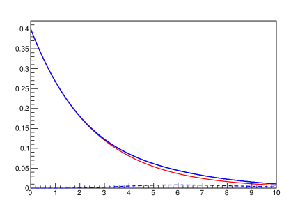
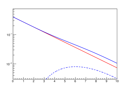
For each hypothesis, the true bin contents $\vec{\mu}$ are then each proportional to the integral of the relevant $f_{\rm true}(y)$ over each bin. For both hypotheses, we take the smearing of $x$ to be the Gaussian resolution function,

$$s(x|y)=\frac{1}{\sqrt{2\pi}\sigma}\exp(-(x-y)^{2}/2\sigma^{2}),$$ (6)

where $\sigma$ is known.

For baseline plots, we use the values shown in Table 1, and the study the effect of varying one parameter at a time. For both $x$ and $y$, we consider histograms with 10 bins of width 1 spanning the interval [0,10]. The default $\sigma$ is half this bin width. The quantities $\vec{\mu}$, $R$, and $\vec{\nu}$ are then readily computed as in Ref. [3]. Figure 2 displays $\vec{\mu}$ and $\vec{\nu}$ (in solid histograms), while Fig. 3 displays the response matrix as well as the source bin of events that are observed in each bin. In each simulated experiment, the total number of events is sampled from a Poisson distribution with mean given in Table 1.

Table 1: Values of parameters used in the baseline unfolding examples

Parameter	Baseline value
Amplitude $B$ of departure from null	0.05
Exponential decay parameter $\tau$	2.5
Mean number of events in each simulated experiment	1000
Number of histogram bins	10
Bin width	1.0
Gaussian $\sigma$ for smearing	0.5
Number of events used to construct $R$	$10^{7}$
Number of iterations in EM unfolding	4

Figure 2: Solid histograms: the true bin contents for unsmeared $\vec{\mu}$ and smeared $\vec{\nu}$, for (left) the null hypothesis $H_{0}$ and (right) the alternative hypothesis $H_{1}$. Data points: In MC simulation a set $\{y\}$ of true points is chosen randomly and then smeared to be the set $\{x\}$. The three points plotted in each bin are then the bin contents when $y$ and $x$ are binned, followed by the unfolded estimate for bin contents.

Figure 3: (left) The response matrix $R$ for default parameter values in Table 1. (right) For each bin in the measured $y$ value, the fraction of events that come from that bin (dominant color) and from nearby bins.

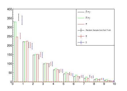
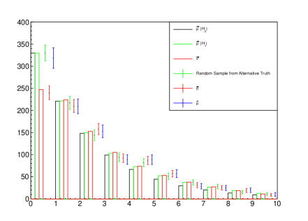
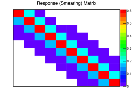
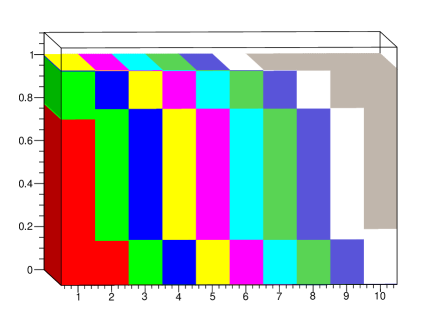
Boundary effects at the ends of the histogram are an important part of a real problem. In our simplified toy problems, we use the same smearing for events near boundaries as for all events (hence not modeling correctly some physical situations where observed values cannot be less than zero); events that are smeared to values outside the histogram are considered lost and contribute to the inefficiencies included in $R$.

These toy models capture some important aspects of real problems in HEP. For example, one might be comparing event generators for top-quark production in the Standard Model. The variable $y$ might be the transverse momentum of the top quark, and the two hypotheses might be two calculations, one to higher order.

Another real problem might be where $y$ represents transverse momentum of jets, the null hypothesis is the standard model, and the alternative hypothesis is some non-standard-model physics that turns on at high transverse momentum. (In this case, it is typically not the case that amplitude $B$ of additional physics is known.)

3 Hypothesis tests in the smeared space

In a typical search for non-standard-model physics, the hypothesis test of $H_{0}$ vs. $H_{1}$ is formulated in the smeared space, i.e., by comparing the histogram contents $\vec{n}$ to the mean bin contents $\vec{\nu}$ predicted by the true densities $f_{\rm true}(y)$ under each hypothesis combined with the resolution function and any efficiency losses. The likelihood ${\cal L}(H_{0})$ for the null hypothesis is the product over bins of the Poisson probability of obtaining the observed bins counts:

$${\cal L}(H_{0})=\prod_{i}P(n_{i};\nu_{i}),$$ (7)

where the $\nu_{i}$ are taken from the null hypothesis prediction. Likelihoods for other hypotheses, such as ${\cal L}(H_{1})$, are constructed similarly.

For testing goodness of fit, it can be useful [4, 5] to use the observed data to construct a third hypothesis, $H_{\rm sat}$, corresponding the saturated model [7], which sets the predicted mean bin contents to be exactly those observed. Thus ${\cal L}(H_{\rm sat})$ is the upper bound on ${\cal L}(H)$ for any hypothesis, given the observed data. The negative log-likelihood ratio

$$-2\ln\lambda_{0,{\rm sat}}=-2\ln\left(\frac{{\cal L}(H_{0})}{{\cal L}(H_{\rm sat})}\right)$$ (8)

is a goodness-of-fit test statistic that is asymptotically distributed as a chisquare distribution if $H_{0}$ is true. Similarly one has $-2\ln\lambda_{1,{\rm sat}}$ for testing $H_{1}$.

An alternative (in fact older) goodness-of-fit test statistic is Pearson’s chisquare [5],

$$\chi^{2}_{\rm P}=\sum_{i=1}^{N}\frac{(n_{i}-\nu_{i})^{2}}{\nu_{i}}.$$ (9)

Yet another alternative, generally less favored, is known as Neyman’s chisquare [4],

$$\chi^{2}_{\rm N}=\sum_{i=1}^{N}\frac{(n_{i}-\nu_{i})^{2}}{n_{i}}.$$ (10)

Ref. [4] argues that Eqn. 8 is the most appropriate GOF statistic for Poisson-distributed histograms, and we use it as our reference point in the smeared space.

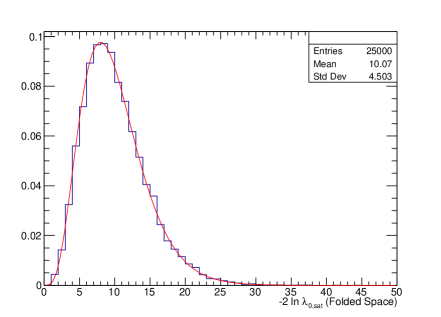
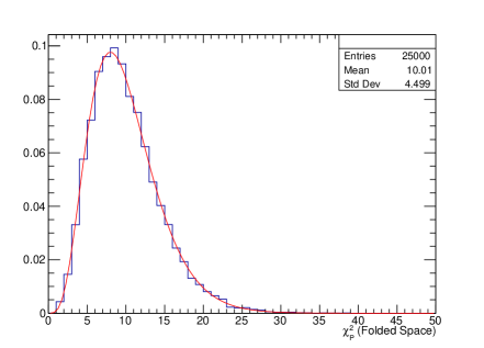
Figure 4 shows the distributions of $-2\ln\lambda_{0,{\rm sat}}$ and $\chi^{2}_{\rm P}$, and their difference, for histograms generated under $H_{0}$. Both distributions follow the expected $\chi^{2}$ distribution with 10 degrees of freedom (DOF). In contrast, the histogram of $\chi^{2}_{\rm N}$ (Figure 4 (bottom left)) has noticeable differences from the theoretical curve.

Figure 4: For events generated under $H_{0}$, in the smeared space with default value of Gaussian $\sigma$, histograms of the GOF test statistics: (top left) $-2\ln\lambda_{0,{\rm sat}}$, (top right) $\chi^{2}_{\rm P}$, and (bottom left) $\chi^{2}_{\rm N}$. The solid curves are the chisquare distribution with 10 DOF. (bottom right) Histogram of the event-by-event difference in the two GOF test statistics $\chi^{2}_{\rm P}$ and $-2\ln\lambda_{0,{\rm sat}}$.

For testing $H_{0}$ vs. $H_{1}$, a suitable test statistic is the likelihood ratio $\lambda$ formed from the probabilities of obtaining bin contents $\vec{n}$ under each hypothesis:

$$-2\ln\lambda_{0,1}=-2\ln\left(\frac{{\cal L}(H_{0})}{{\cal L}(H_{1})}\right)=-2\ln\lambda_{0,{\rm sat}}-(-2\ln\lambda_{1,{\rm sat}}\,),$$ (11)

where the second equality follows from Eqn. 8. Figure 5 shows the distribution of $-2\ln\lambda_{0,1}$ for events generated under $H_{0}$ and for events generated under $H_{1}$, using the default parameter values in Table 1.

Figure 5: In the smeared space, histogram of the test statistic $-2\ln\lambda_{0,1}$ for events generated under $H_{0}$ (in blue) and $H_{1}$ (in red).

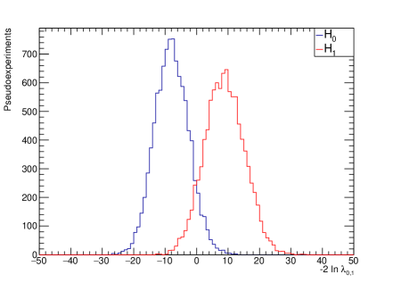
We would assert that these results obtained in the smeared space are the “right answers” for chisquare-like GOF tests of $H_{0}$ and $H_{1}$ (if desired), and in particular for the likelihood-ratio test of $H_{0}$ vs $H_{1}$ in Fig. 5. Given a particular observed data set, such histograms can be used to calculate $p$-values for each hypothesis, simply by integrating the appropriate tail of the histogram beyond the observed value of the relevant likelihood ratio [5]. In frequentist statistics, such $p$-values are typically the basis for inference, especially for the simple-vs-simple hypothesis tests considered here. (Of course there is a vast literature questioning the foundations of using $p$-values, but in this note we assume that they can be useful, and are interested in comparing ways to compute them.)

We compare $-2\ln\lambda$, $\chi^{2}_{\rm P}$, $\chi^{2}_{\rm N}$, and the generalization of Eqn. 12 including correlations in various contexts below. For Poisson-distributed data, arguments in favor of $-2\ln\lambda$ when it is available are in Ref. [4].

3.1 Note regarding Gaussian data and the usual $\chi^{2}$ GOF test

In the usual $\chi^{2}$ GOF test with (uncorrelated) estimates $\hat{\vec{\nu}}$ having Gaussian densities with standard deviations $\vec{\sigma}$, one would commonly have

$$\chi^{2}=\sum_{i=1}^{N}\frac{(\hat{\nu}_{i}-\nu_{i})^{2}}{\sigma_{i}^{2}}.$$ (12)

Although not usually mentioned, this is equivalent to a likelihood ratio test with respect to the saturated model, just as in the Poisson case. The likelihood is

$${\cal L}=\prod_{i}\frac{1}{\sqrt{2\pi\sigma_{i}^{2}}}\exp\left(-(\hat{\nu}_{i}-\nu_{i})^{2}/2\sigma_{i}^{2}\right),$$ (13)

where for ${\cal L}(H_{0})$ one has $\nu_{i}$ predicted by $H_{0}$, and for the saturated model, one has $\nu_{i}=\hat{\nu}_{i}$. Thus

$${\cal L}(H_{\rm sat})=\prod_{i}\frac{1}{\sqrt{2\pi\sigma_{i}^{2}}},$$ (14)

and hence $\chi^{2}=-2\ln({\cal L}(H_{0})/{\cal L}(H_{\rm sat}))=-2\ln\lambda_{0,{\rm sat}}.$ (It is sometimes said loosely and incorrectly that for the Gaussian model, $\chi^{2}=-2\ln{\cal L}(H_{0})$, but clearly the ratio is necessary to cancel the normalization factor.)

There is also a well-known connection between the usual Gaussian $\chi^{2}$ of Eqn. 12 and Pearson’s chisquare in Eqn. 9: since the variance of a Poisson distribution is equal to its mean, a naive derivation of Eqn. 9 follows immediately from Eqn. 12. If one further approximates $\nu_{i}$ by the estimate $n_{i}$, then one obtains Neyman’s chisquare in Eqn. 10.

4 Unfolding by using maximum likelihood estimates and approximations from truncated iterative solutions

If one unfolds histograms and then compares the unfolded histograms $\hat{\vec{\mu}}$ to (never smeared) model predictions $\mu$, even informally, then one is implicitly assuming that the comparison is scientifically meaningful. For this to be the case, we would assert that the results of comparisons should not differ materially from the “right answers” obtained above in the smeared space. Here we explore a few test cases.

Given the observed histogram contents $\vec{n}$, the likelihood function for the unknown $\vec{\nu}$ follows from Eqn. 2 and leads to the maximum likelihood (ML) estimates $\hat{\nu}_{i}=n_{i}$, i.e.,

$$\hat{\vec{\nu}}=\vec{n}.$$ (15)

One might then expect that the ML estimates of the unknown means $\vec{\mu}$ can be obtained by substituting $\hat{\vec{\nu}}$ for $\vec{n}$ in Eqn. 1. If $R$ is a square matrix, as assumed here, then this yields

$$\hat{\vec{\mu}}=R^{-1}\,\hat{\vec{\nu}}=R^{-1}\,\vec{n}.$$ (16)

These are indeed the ML estimates of $\vec{\mu}$ as long as $R$ is invertible and the estimates $\mu_{i}$ are positive [3, 8], which is generally the case in the toy problem studied here.

The covariance matrix of the estimates $\hat{\vec{\mu}}$ in terms of $R$ and $\vec{\nu}$ is derived in Ref. [3]:

$$U=R^{-1}\,V\,(R^{-1})^{T},$$ (17)

where $V_{ij}=\delta_{ij}\nu_{i}$. Since the true values $\vec{\nu}$ are presumed unknown, it is natural to substitute the estimates from Eqn. 15, thus obtaining an estimate $\hat{U}$. Consequences of this approximation are discussed below.

In all cases (even when matrix inversion fails), the ML estimates for $\vec{\mu}$ can be found to desired precision by the iterative method variously known as [8] Expectation Maximization (EM), Lucy-Richardson, or (in HEP) the iterative method of D’Agostini [9]. Because the title of Ref. [9] mentions Bayes’ Theorem, in HEP the EM method is unfortunately (and wrongly) referred to as “Bayesian”, even though it is a fully frequentist algorithm [8].

As discussed by Cowan [3], the ML estimates are unbiased, but the unbiasedness can come at a price of large variance that renders the unfolded histogram unintelligible to humans. Therefore there is a vast literature on “regularization methods” that reduce the variance at the price of increased bias, such that the mean-squared-error (the sum of the bias squared and the variance) is (one hopes) reduced.

The method of regularization popularized in HEP by D’Agostini [9] (and studied for example by Bohm and Zech [10]) is simply to stop the iterative EM method before it converges to the ML solution. The estimates $\hat{\vec{\mu}}$ then retain some memory of the starting point of the solution (typically leading to a bias) and have lower variance. The uncertainties (covariance matrix) also depend on when the iteration stops.

Our studies in this note focus on the ML and truncated iterative EM solutions, and use the EM implementation (unfortunately called RooUnfoldBayes) in the RooUnfold [11] suite of unfolding tools. This means that for the present studies, we are constrained by the policy in RooUnfold to use the “truth” of the training sample to be the starting point for the iterative EM method; thus we have not studied convergence starting from, for example, a uniform distribution. Useful studies of the bias of estimates are thus not performed.

Other popular methods in HEP include variants of Tikhonov regularization, such as “SVD” method advocated by Hocker and Kartvelishvili [12], and the implementation included in TUnfold [13]. The relationship of these methods to those in the professional statistics literature is discussed by Kuusela [8].

Figure 2 shows (in addition to the solid histograms mentioned above) three points with error bars plotted in each bin, calculated from a particular set of simulated data corresponding to one experiment. The three points are the bin contents when the sampled values of $y$ and $x$ are binned, followed by that bin’s components of the set of unfolded estimates $\hat{\vec{\mu}}$. Figure 6(left) shows the covariance matrix $\hat{U}$ for the estimates $\hat{\vec{\mu}}$ obtained for the same particular simulated data set, unfolded by matrix inversion (Eqn. 16) to obtain the ML estimates. Figure 6 (right) shows the corresponding correlation matrix with elements $\hat{U}_{ij}/\sqrt{\hat{U}_{ii}\hat{U}_{jj}}$. Figure 7 shows the corresponding matrices obtained when unfolding by the iterative EM method with default number of iterations. For the ML solution, adjacent bins are negatively correlated, while for the EM solution with default (4) iterations, adjacent bins are positively correlated due to the implicit regularization.

Figure 6: (left) covariance matrix $\hat{U}$ for unfolded estimates, as provided by the ML estimates (matrix inversion). (right) The correlation matrix corresponding to $\hat{U}$, with elements $\hat{U}_{ij}/\sqrt{\hat{U}_{ii}\hat{U}_{jj}}$.

Figure 7: (left) covariance matrix $\hat{U}$ for unfolded estimates, as provided by the default iterative EM method. (right) The correlation matrix corresponding to $\hat{U}$, with elements $\hat{U}_{ij}/\sqrt{\hat{U}_{ii}\hat{U}_{jj}}$.

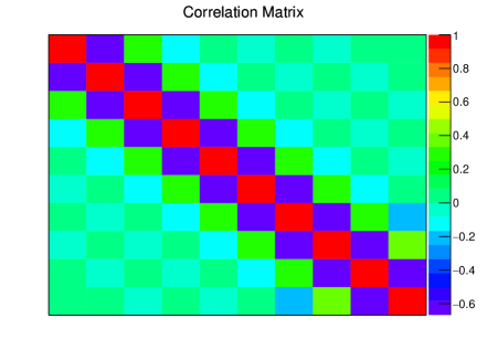
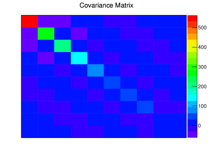
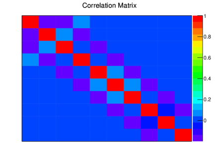
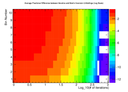
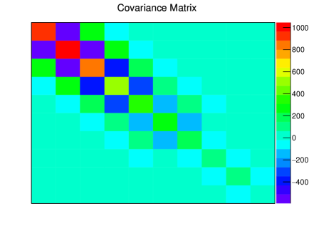
Figure 8 shows an example of the convergence of iterative EM unfolding to the ML solution for one simulated data set. On the left is the fractional difference between the EM and ML solutions, for each of the ten histogram bins, as a function of the number of iterations, reaching the numerical precision of the calculation. On the right is the covariance matrix $\hat{U}$ after a large number of iterations, showing convergence to that obtained by matrix inversion in Fig. 6(left).

Figure 8: (left) Fractional difference between the EM and ML solutions, for each of the ten histogram bins, as a function of the number of iterations. (right) The covariance matrix of the EM method after a large number of iterations, to be compared to the ML solution in Fig. 6(left).

5 Hypothesis tests in the unfolded space

Although the ML solution for $\hat{\vec{\mu}}$ may be difficult for a human to examine visually, if the covariance matrix $U$ is well enough behaved, then a computer can readily calculate a chisquare GOF test statistic in the unfolded space by using the generalization of Eqn. 12, namely the usual formula for GOF of Gaussian measurements with correlations [5],

$$\chi^{2}_{\rm corr}=(\hat{\vec{\mu}}-\vec{\mu})^{T}\,U^{-1}\,(\hat{\vec{\mu}}-\vec{\mu}).$$ (18)

If unfolding is performed by matrix inversion (when equal to the ML solution), then substituting $\hat{\vec{\mu}}=R^{-1}\,\vec{n}$ from Eqn. 16, $\vec{\mu}=R^{-1}\,\vec{\nu}$ from Eqn. 1, and $U^{-1}=R^{T}\,V^{-1}\,R$ from Eqn. 17, yields

$$\chi^{2}_{\rm corr}=(\vec{n}-\vec{\nu})^{T}\,V^{-1}\,(\vec{n}-\vec{\nu}).$$ (19)

So for $V_{ij}=\delta_{ij}\nu_{i}$ as assumed by Cowan, this $\chi^{2}_{\rm corr}$ calculated in the unfolded space is equal to Pearson’s chisquare (Eqn. 9) in the smeared space.

If however one substitutes $\hat{\vec{\nu}}=\vec{n}$ for $\vec{\nu}$ as in Eqn. 15, then $\chi^{2}_{\rm corr}$ in the unfolded space is equal to Neyman’s chisquare in the smeared space! This is the case in the implementation of RooUnfold that we are using, as noted below in the figures.

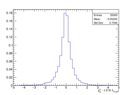
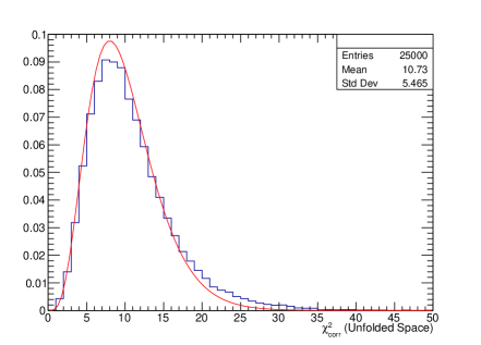
For events unfolded with the ML estimates, Figure 9 (top left) shows the results of such a $\chi^{2}_{\rm corr}$ GOF test with respect to the null hypothesis using same events used in Fig. 4. As foreseen, the histogram is identical (apart from numerical artifacts) with the histogram of $\chi^{2}_{\rm N}$ in Fig. 4 (bottom left). Figure 9 (top right) show the event-by-event difference of $\chi^{2}_{\rm corr}$ and Pearson’s $\chi^{2}$ in the smeared space, and Figure 9 (bottom) is the difference with respect to $-2\ln\lambda_{0,{\rm sat}}$ in the smeared space. Figure 10 shows the same quantities calculated after unfolding using the iterative EM method with default iterations.

For these tests using ML unfolding, the noticeable difference between the GOF test in the smeared space with that in the unfolded space is directly traced to the fact that the test in the unfolded space is equivalent to $\chi^{2}_{\rm N}$ in the smeared space, which is an inferior GOF test compared to the likelihood ratio test statistic $-2\ln\lambda_{0,sat}$. It seems remarkable that, even though unfolding by matrix inversion would appear not to lose information, in practice the way the information is used (linearizing the problem via expressing the result via a covariance matrix) already results in some failures of the bottom-line test of GOF. This is without any regularization or approximate EM inversion.

Figure 9: Quantities calculated after unfolding using ML estimates. (top left) Histograms of generalized GOF test statistic $\chi^{2}_{\rm corr}$ that tests for compatibility with $H_{0}$ in the unfolded space, for the same events generated under $H_{0}$ as those used in the smeared-space test of Fig. 4. (top right) For these events, histogram of the difference between $\chi^{2}_{\rm corr}$ in the unfolded space and $\chi^{2}_{\rm P}$ in the smeared space. (bottom) For these events, histogram of the difference between $\chi^{2}_{\rm corr}$ in the unfolded space and the GOF test statistic $-2\ln\lambda_{0,sat}$ in the smeared space.

Figure 10: The same quantities as in Fig. 9, here calculated after unfolding using the iterative EM method with default (four) iterations.

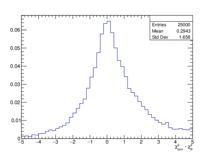
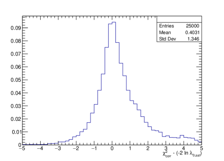
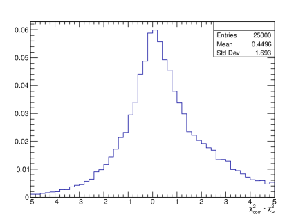
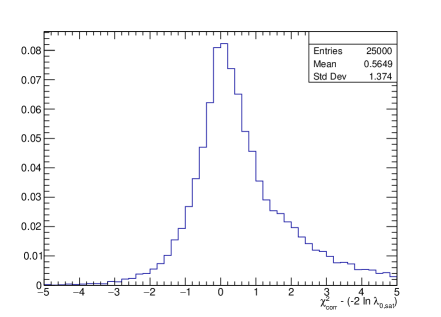
For the histogram of each simulated experiment, the GOF statistic $\chi^{2}_{\rm corr}$ is calculated with respect to the prediction of $H_{0}$ and also with respect to the prediction of $H_{1}$. The difference of these two values, $\Delta\chi^{2}_{\rm corr}$, is then a test statistic for testing $H_{0}$ vs. $H_{1}$, analogous to the test statistic $-2\ln\lambda_{0,1}$. Figure 11 shows, for the same events as those used in Fig. 5, histograms of the test statistic $\Delta\chi^{2}_{\rm corr}$ in the unfolded space for events generated under $H_{0}$ and under $H_{1}$, with $R$ calculated using $H_{0}$ and using $H_{1}$. For the default problem studied here, the dependence on $R$ is not large. Thus unless otherwise specified, all other plots use $R$ calculated under $H_{0}$.

Figure 11: (left) For the same events as those used in Fig. 5, histogram of the test statistic $\Delta\chi^{2}_{\rm corr}$ in the unfolded space, for events generated under $H_{0}$ (in blue) and $H_{1}$ (in red), with $R$ calculated using $H_{0}$. (right) For the same events, histograms of the test statistic $\Delta\chi^{2}_{\rm corr}$ in the unfolded space, with $R$ calculated using $H_{1}$.

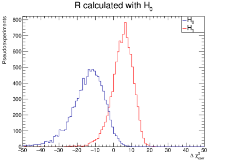
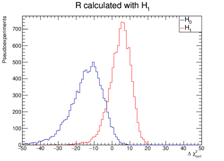
Figure 12 shows, for the events in Figs. 5 and in 11, histograms of the event-by-event difference of $-2\ln\lambda_{0,1}$ and $\Delta\chi^{2}_{\rm corr}$. The red curves correspond to events generated under $H_{0}$, while the blue curves are for events generated under $H_{1}$. The unfolding method is ML on the left and iterative EM on the right. This is an example of a bottom-line test: does one obtain the same answers in the smeared and unfolded spaces? There are differences apparent with both unfolding techniques. Since the events generated under both $H_{0}$ and $H_{1}$ are shifted in the same direction, the full implications are not immediately clear. Thus we turn to ROC curves or equivalent curves from Neyman-Pearson hypothesis testing.

Figure 12: For the events in Figs. 5 and in 11(left), histogram of the event-by-event difference of $-2\ln\lambda_{0,1}$ and $\Delta\chi^{2}_{\rm corr}$. In the left histogram, ML unfolding is used, while in the right histogram, iterative EM unfolding is used.

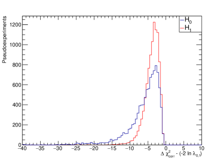
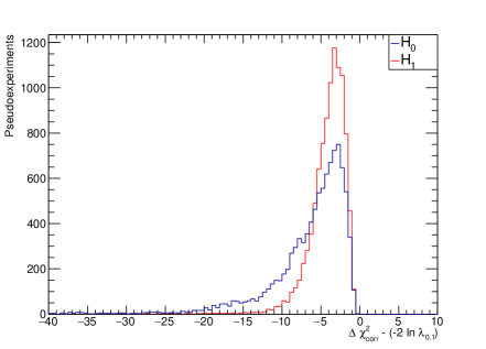
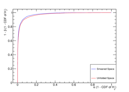
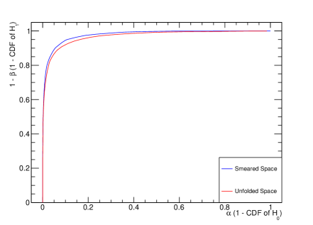
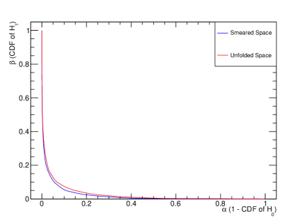
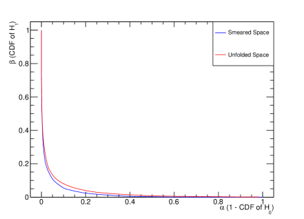
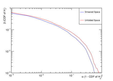
We can investigate the effect of the differences apparent in Fig. 12 by using the language of Neyman-Pearson hypothesis testing, in which one rejects $H_{0}$ if the value of the test statistic ($-2\ln\lambda_{0,1}$ in the smeared space, or $\Delta\chi^{2}_{\rm corr}$ in the unfolded space) is above some critical value [6]. The Type I error probability $\alpha$ is the probability of rejecting $H_{0}$ when it is true, also known as the “false positive rate”. The Type II error probability $\beta$ is the probability of accepting (not rejecting) $H_{0}$ when it is false. The quantity $1-\beta$ is the power of the test, also known as the “true positive rate”. The quantities $\alpha$ and $\beta$ thus follow from the cumulative distribution functions (CDFs) of histograms of the test statistics. In classification problems outside HEP is it common to make the ROC curve of true positive rate vs. the false positive rate, as shown in Fig. 13. Figure 14 shows the same information in a plot of $\beta$ vs. $\alpha$, i.e., with the vertical coordinate inverted compared to the ROC curve. Figure 15 is the same plot as Fig. 14, with both axes having logarithmic scale.

The result of this “bottom line test” does not appear to be dramatic in this first example, and appear to be dominated by the difference between the Poisson-based $-2\ln\lambda_{0,1}$ and $\Delta\chi^{2}_{\rm corr}$ already present in the ML unfolding solution, rather than by the additional differences caused by truncating the EM solution. Unfortunately no general conclusion can be drawn from this observation, since as mentioned above the EM unfolding used here starts from the true distribution as the first estimate. It is of course necessary to study other initial estimates.

Figure 13: For the events in Figs. 5 and 11(left), ROC curves for classification performed in the smeared space (blue curve) and in the unsmeared space (red curve). (left) unfolding by ML, and (right) unfolding by iterative EM.

Figure 14: For the events in Figs. 5 and 11(left), plots of $\beta$ vs. $\alpha$, for classification performed in the smeared space (blue curve) and in the unsmeared space (red curve). (left) unfolding by ML, and (right) unfolding by iterative EM.

Figure 15: The same plot of $\beta$ vs. $\alpha$ as in Fig. 14, here with logarithmic scale on both axes.

5.1 Variation of parameters from the default values

With the above plots forming a baseline, we can ask how some of the above plots vary as we change the parameters in Table 1.

Figure 16 shows, as a function of the Gaussian smearing parameter $\sigma$, the variation of the GOF results shown for $\sigma=0.5$ in 1D histograms in Figs. 9 (top left) and 9 (bottom). The events are generated under $H_{0}$.

Figure 16: For iterative EM unfolding, variation of GOF results with the Gaussian $\sigma$ used in smearing (vertical axis). The horizontal axes are the same as those in the 1D histograms in Figs. 9 (top left) and 9 (bottom), namely $\chi^{2}_{\rm corr}$ in the unfolded space; and the difference with respect to $-2\ln\lambda_{0,{\rm sat}}$ in the smeared space; for GOF tests with respect to $H_{0}$ using events generated under $H_{0}$.

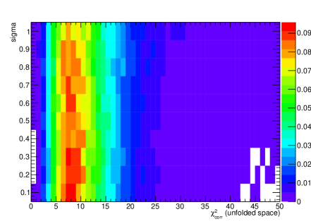
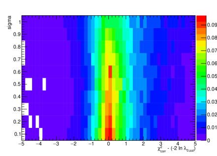
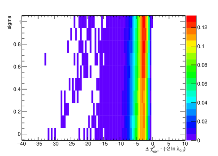
Figure 17 shows the variation of the 1D histogram in Fig 12 with the Gaussian $\sigma$ used in smearing, for both ML and EM unfolding.

Figure 17: (left) For unfolding by ML estimates, variation with the Gaussian $\sigma$ used in smearing (vertical axis) of the 1D histogram in Fig 12 of the event-by-event difference of $-2\ln\lambda_{0,1}$ and $\Delta\chi^{2}_{\rm corr}$. (right) the same quantity for iterative EM unfolding.

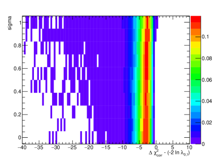
Figures 18 and 19 show, for ML and EM unfolding respectively, the result of the bottom-line test of Fig. 12 as a function of the amplitude $B$ of the extra term in $f_{\rm true,1}$ in Eqn. 4.

Figure 18: The result of the bottom-line test of Fig. 12 as a function of the amplitude $B$ of the extra term in $f_{\rm true,1}$ in Eqn. 4, for (left) $R$ derived from $H_{0}$ and (right) $R$ derived from $H_{1}$; for ML unfolding.

Figure 19: The same as Fig. 18, for iterative EM unfolding.

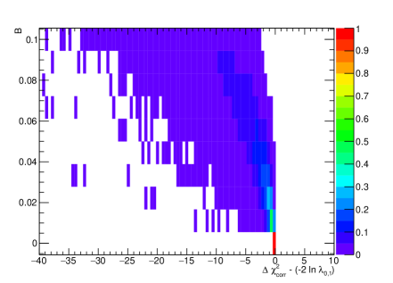
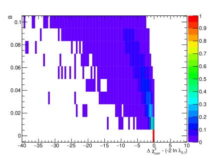
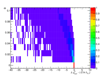
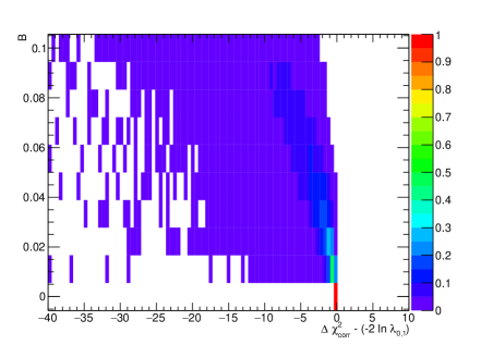
Figure 20 shows, for ML and EM unfolding, the result of the bottom-line test of Fig. 12 as a function of the mean number of events in the histogram of $\vec{n}$.

Figure 20: The result of the bottom-line test of Fig. 12 as a function of the number of events on the histogram of $\vec{n}$, for (left) ML unfolding and (right) iterative EM unfolding.

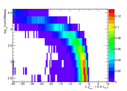
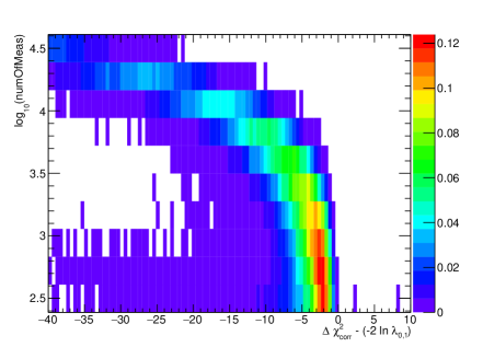
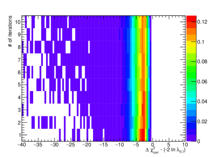
Figure 21 shows, for iterative EM unfolding, the result of the bottom-line test of Fig. 12 as a function of the number of iterations.

Figure 21: For EM iterative unfolding, the result of the bottom-line test of Fig. 12 as a function of number of iterations in (left) linear vertical scale and (right) logarithmic vertical scale.

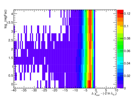
6 Discussion

This note illustrates in detail some of the differences that can arise with respect to the smeared space when testing hypotheses in the unfolded space. As the note focuses on a particularly simple hypotheses test, and looks only at the ML and EM solutions, no general conclusions can be drawn, apart from claiming the potential usefulness of the “bottom line tests”. Even within the limitations of the RooUnfold software used here (in particular that the initial estimate for iterating is the presumed truth), we see indications of dangers of testing hypotheses after unfolding. Perhaps the most interesting thing to note thus far is that unfolding by matrix inversion (and hence no regularization) yields, in the implementation studied here, a generalized $\Delta\chi^{2}_{\rm corr}$ test statistic that is identical to $\chi^{2}_{\rm N}$ in the smeared space, which is intrinsically inferior to $-2\ln\lambda_{0,1}$. The potentially more important issue of bias due to regularization affecting the bottom line test remains to be explored.

Such issues should be kept in mind, even in informal comparisons of unfolded data to predictions from theory. For quantitative comparison (including the presumed use of unfolded results to evaluate predictions in the future from theory), we believe that extreme caution should be exercised, including performing the bottom-line-tests with various departures from expectations. This applies to both GOF tests of a single hypothesis, and comparisons of multiple hypotheses.

More work is needed in order to gain experience regarding what sort of unfolding problems and unfolding methods yield results that give reasonable performance under the bottom-line-test, and which cases lead to bad failures. As often suggested, reporting the response matrix $R$ along with the smeared data can facilitate comparisons with future theories in the folded space, in spite of the dependence of $R$ on the true pdfs.