e-Distance Weighted Support Vector Regression
Abstract
We propose a novel support vector regression approach called e-Distance Weighted Support Vector Regression (e-DWSVR). e-DWSVR specifically addresses two challenging issues in support vector regression: first, the process of noisy data; second, how to deal with the situation when the distribution of boundary data is different from that of the overall data. The proposed e-DWSVR optimizes the minimum margin and the mean of functional margin simultaneously to tackle these two issues. In addition, we use both dual coordinate descent (CD) and averaged stochastic gradient descent (ASGD) strategies to make e-DWSVR scalable to large-scale problems. We report promising results obtained by e-DWSVR in comparison with existing methods on several benchmark datasets.
1 Introduction
Support Vector Regression (SVR) has recently received much attention due to its competitive performance [1][2] compared with other regression approaches, including the method of least squares [3], the XCSF algorithm [4], the logistic regression [5], and Neural Networks (NN) [6]. In this paper, we aim to develop a novel SVR approach by considering the recent progress in the support vector (SV) theory and addressing the limitations of existing SVR approaches.
In general, SVR constructs decision functions in high dimensional space for linear regression while the training data are mapped to a higher dimension in kernel Hilbert space. -SVR [7][8] (the symbol is replaced by e in the rest of this paper, and thus e-SVR is used) is the first popular SVR strategy and the other one is v-SVR [9]. e-SVR aims to find a function whose deviation is not more than e, thus forming the so-called e-tube, to fit all training data. In order to find the best fitting surface, e-SVR tries to maximize the minimum margin containing data points in the e-tube as much as possible, which is similar to SVM. As for v-SVR, it adds a parameter v to the original e-SVR to control the number of support vectors and adjust the parameter e automatically [10].
However, both e-SVR and v-SVR are susceptible to the data on the boundary (i.e. the support vectors). In fact, the optimization objective greatly depends on the margin between support vectors, and this makes the final fitting function heavily rely on the distribution of the support vectors: if the distribution of the whole data within the e-tube is very different from the direction of the support vectors, the final regression function may not be reliable.
Recent progress in the SV theory suggests that maximizing the minimum margin, that is, the shortest distance from the instances to the separating hyperplane, is not the only optimization goal for achieving better learning performance. Different from traditional SVMs, Distance-weighted Discrimination (DWD)[11] maximizes the mean of the functional margin of all data [12], and it uses the distances of all data to define the separating hyperplane, thus greatly improving the performance. Meanwhile, Large Margin Distribution Machine (LDM) [13][14] is based on the novel theory of minimizing the margin distribution, and it employed the dual coordinate descent (CD) and the averaged stochastic gradient descent (ASGD) strategies to solve the optimization function.
Considering the above, we propose a novel SVR approach called e-Distance Weighted Support Vector Regression (e-DWSVR). e-DWSVR optimizes the minimum margin and the mean of functional margin at the same time, and it also uses both CD and ASGD strategies as in LDM to improve its scalability. A comparison of our e-DWSVR with several other popular regression methods (including e-SVR, NN, linear regression and logistic) indicates that our e-DWSVR fits better the whole data distribution in most cases, especially for those datasets with strong interference noise.
2 Background on support vector theory
Let be a training set of samples, where are the input samples and are the corresponding target values. For regression, the objective function is , where and is the mapping function induced by a kernel , i.e., , which projects the data to a higher dimensional space.
2.1 The e-SVR process.
According to [7][8], the objective function is represented by the following constrained minimization problem:
In the above, is a parameter that denotes the trade-off between the flatness of and sums up to which deviations larger than e are tolerated. and are regarded as the slack variables measuring the distances of the training samples lying outside the e-tube from the tube itself. After applying the Lagrange multiplier, the minimization problem can be handled as the dual optimization problem:
And the final objective function becomes
2.2 Recent progress in the SV theory
SVM aims to maximize the minimum margins, which denotes the smallest distances of all instances to the separating hyperplane [1][2]. The optimization problem is represented as follows:
The DWD method [11] uses a new criterion for the optimization problem [12]. We denote the functional margin as and let be the adjusted distance of the -th data to the separating hyperplane. So the solution of DWD is given below:
Furthermore, the LDM method optimizes the margin distribution to solve the optimization problem [13][14]. Thus the optimization problem becomes
| (1) |
where , , is the label set. LDM offers two strategies to solve Formula (1): for small and medium datasets, Formula (1) can be solved by the CD method [13], and for large-scale problem, ASGD is used [13][15][16]. ASGD solves the optimization objective by computing a noisy unbiased estimate of the gradient and it randomly samples a subset of the training instances rather than all the data. Our method uses a similar implementation of the CD and ASGD methods, which will be introduced in detail in the next section.
3 The proposed e-DWSVR
In this section, we describe the novel e-DWSVR method, which applies the idea of the mean of functional margin and employs a similar solution as in LDM, that is, we use the CD strategy to handle general conditions and adopt the ASGD strategy to deal with large-scale problems.
3.1 Formulation for e-DWSVR
For regression problems, the input is and the target is , where . In order to simplify the complexity brought by the bias term, we enlarge the dimension of the vectors and to handle the bias term [17], i.e., , . Thus the form of the regression function becomes . Then the margin in the regression analysis will be the distance of a point to the fitting hyperplane, i.e. Based on the concept of margin, we give the definition of functional margin.
Definition 1: functional margin in regression:
The functional margin can describe the difference between the real values and the estimated value. It also has a significant connection with the geometrical distance. In fact, the functional margin is the adjusted distance of the data to the separating hyperplane. If the value of is determined, the ranking of all data points to the fitting surface with respect to the margin can be decided by functional margin. Then the mean of the functional margin in regression is defined by Definition 2 as follows.
Definition 2: mean of the functional margin in regression:
Based on the above definitions, we will not only maximize the minimum margin, but also minimize the mean of the functional margin at the same time, in order to obtain a better tradeoff between the distribution of the whole data and the distribution of support vectors. e-DWSVR considers the influence of all data to the fitting surface, as this is closer to the actual distribution of the internal data.
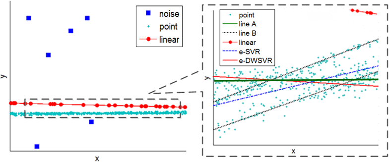
To illustrate the difference of the optimal objectives between e-SVR and e-DWSVR, we use an example for comparison among linear regression, e-SVR and e-DWSVR on an artificial dataset. The distribution of the whole data is shown in Figure 1(a), where those sparse quadrate points are the noise and the red solid line with points is drawn by linear regression. Figure 1(b) is the enlarged version of the dotted box in Figure 1(a) for better observing the differences among the three methods. In Figure 1(b) the points show the distribution of most non-noisy data and the black dotted lines represent the data on the boundary. The red solid line with points is part of the line in Figure 1(a). The blue dashed curve is drawn by e-SVR and the red solid curve is drawn by e-DWSVR.
Obviously, the curve drawn by linear regression is far from the dataset, which indicates that the linear regression is more sensitive to noisy points, and this makes the curve in a wrong direction. e-SVR and e-DWSVR are not affected easily by noise points, so the blue dashed curve and the red solid curve are within area of non-noisy data. However, the regression model implemented by e-SVR is controlled by the support vectors (those boundary points). Once the internal data distribution is different from the edge points (which is the case in Figure 1(b)), the regression model will not achieve good performance. e-SVR produces the blue dashed curve which is different from the red solid curve. Because e-DWSVR considers the influence of all data to the fitting surface, it is obvious the red solid curve drawn by e-DWSVR is closer to the actual distribution of the internal data.
(a) The whole data with noise (b) The distribution of data without noise
As in the soft-margin e-SVR [1], we also consider complicated conditions. So, the final optimization function has the following form:
3.2 e-DWSVR for medium-scale regression with kernel.
Considering the mean of the functional margin in the constrained minimization problem, we can obtain the following form:
| (2) |
Here we omit the term in because it is regarded as a constant in an optimization problem. Obviously, the high dimensionality of and its complicated form makes Formula (2) more intractable. To simplify this formula, we take the suggestion from [18] and the optimal solution in LDM [13]. We first give the following theorem.
Theorem 1. The optimal solution for Formula (2) can be represented as the following form: where and are the parameters of e-DWSVR.
PROOF. We assume that can be divided into the span of and an orthogonal vector, i.e.,
where satisfies for all , that is, Then we obtain the following formula: Hence, the second term of Formula (2) is independent of considering Formula (4). Furthermore, note that the constraints of Formula (2) are also independent of , so the last term of Formula (2) can be considered as independent of . To simplify the first term, we have In the above "" becomes "" if and only if . Thus, setting strictly reduces the first term of Formula (2) without affecting the rest terms. Based on all above, in Formula (2) can be represented in the form of Formula (3). Q.E.D.
According to Theorem 1, Formula (2) can be cast as where , and The minimization problem which has been simplified can be transformed into a dual formulation with the Lagrange multipliers, so the Lagrange function of Formula (5) leads to where are the Lagrange multipliers. To satisfy the KKT condition, we set the partial derivatives to zero and obtain the following formulas: By substituting Formulas (7) and (8) into Formula (6) and inspired by reference [19], Formula (5) can be written as follows to compute the values of separately. where , and stands for the inverse matrix of and means the all-one vector.
So Formula (9) can be solved by the CD method as in [20][21]. This method continuously selects one variable for minimization and keeps others as constants. In our situation, we minimize by fixing other , where , and needs to be solved, where , and the form of this sub-problem is where is the diagonal entry of , and is the -th element of the gradient . Obviously is independent of , so we omit this part of Formula (10). Hence is transformed into a simple quadratic function.
After calculating , we can obtain according to Formula (7) as Therefore, we obtain the final fitting function as
Algorithm 1 presents the detailed steps of the CD method used for efficiently updating .
Input: Dataset , , ,
Output:
Initialization:
3.3 e-DWSVR for large-scale regression.
Although the CD method can solve e-DWSVR efficiently, it is not a best strategy for dealing with large-scale problems. To further improve the scalability of e-DWSVR, we also apply ASGD method to e-DWSVR.
We reformulate Formula (2) as follows to solve large-scale problems,
| (11) |
Computing the gradient of in Formula (11) is time consuming because we need all the training instances for computation. Considering this issue, we use Stochastic Gradient Descent (SGD) [22] to compute a noisy unbiased estimation of the gradient, and this is done by randomly sampling part of the training instances.
Therefore, we give an unbiased estimation of the gradient in our case. For denoting the last term of (11) formally, we define a function that has different values under different constraint conditions, as shown below:
where .
Theorem 2. An unbiased estimation of the gradient has the following form:
where one instance is sampled randomly from the training set.
PROOF: The gradient of has the form , where and . Note that Considering the linearity of expectation, and with Formula (12), we have This leads to a conclusion that is a noisy unbiased estimation of the gradient. Q.E.D.
Then, the stochastic gradient can be updated iteratively with the following form: where is the learning rate at the -th iteration.
The good choice for can be obtained by the form by ASGD, where , , and are constants [23]. And we compute at each iteration in addition to updating the ordinary stochastic gradient in Formula (13) as , where decides when to perform the averaging process. This average can also be calculated in a recursive manner as , where is the rate of averaging and
Finally, Algorithm 2 provides the detailed steps of ASGD for large-scale problems, where determines the number of iteration. means the adjustment of the whole times of iteration which is set as same as [13]; means , and its initial value is 0.
Input: Dataset , ,
Output:
Initialization:
4 Experiments
In this section, we report the effectiveness of e-DWSVR in comparison with other regression methods to assess whether our method has better fitting quality.
4.1 Experimental setup
We select sixteen datasets from UCI [24] to evaluate these methods. This includes eight medium-scale datasets and eight large-scale datasets. The numbers of samples and features for each dataset are indicated in Table 1 and 2. For instance, Slump (103 / 7) means the sample size is 103 and the number of features is 7 for the Slump dataset. All features of datasets and target set are normalized into [0,1] for balancing the influence of each feature. After normalization, we take a preprocess of the PCA with the contribution to 95% for feature extraction. During the construction of the regression model, we divide the datasets into training sets and testing sets by 5-fold cross validation, and the experiments are repeated for 30 times. For medium-scale datasets, we evaluate both the linear and RBF kernels [1], and the average values and standard deviation are recorded. For large-scale datasets, only the linear kernel is evaluated. In addition, we record the time cost.
e-SVR, NN [6], linear regression and logistic are compared with our method. For e-SVR and e-DWSVR, parameters and are both needed when building models. So these parameters are optimized during the experiments to select the best parameters for regression. For e-DWSVR, parameter is fixed to 1; parameter , , and have the same values as in [13]. All optimization are processed on testing sets.
The mean square error (MSE) [25] and R-square (R2) [26] are commonly used evaluation metrics in regression, and thus they are chosen in our research for evaluation. All experiments are tested with MATLAB on a PC, which has a 2.50 GHz CPU and 8 GB memory.
4.2 Result and discussion
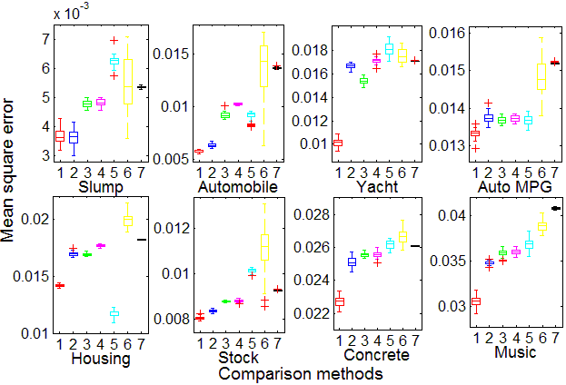
For medium-scale datasets, Figure 1 shows the results of MSE on all methods, including linear kernel function and RBF kernel function for e-DWSVR and e-SVR. Table 1 summarizes the results of R2 on all methods. In most datasets, e-DWSVR performs better than other methods. Obviously, the fitting quality of e-DWSVR is much better than e-SVR, which means e-DWSVR is more competitive than e-SVR. In Table 2, the best R2 on each dataset is indicated in bold.
|
|
|
|
|
LINEAR | NN | Logistic | ||||||||||
|---|---|---|---|---|---|---|---|---|---|---|---|---|---|---|---|---|---|
| Slump (103 / 7) | 0.9539 | 0.9224 | 0.8739 | 0.8641 | 0.8067 | 0.8220 | 0.8336 | ||||||||||
| Automobile (205 / 26) | 0.8865 | 0.8320 | 0.7847 | 0.7689 | 0.7748 | 0.7526 | 0.7592 | ||||||||||
| Yacht (308 / 7) | 0.8684 | 0.7526 | 0.7397 | 0.7083 | 0.6574 | 0.6990 | 0.7007 | ||||||||||
| Auto MPG (398 / 8) | 0.6900 | 0.6874 | 0.6839 | 0.6837 | 0.6843 | 0.6782 | 0.6673 | ||||||||||
| Housing (506 / 14) | 0.6955 | 0.6634 | 0.6851 | 0.6522 | 0.7048 | 0.6091 | 0.6326 | ||||||||||
| Stock (536 / 9) | 0.5687 | 0.5566 | 0.5344 | 0.5241 | 0.4055 | 0.3719 | 0.4146 | ||||||||||
| Concrete (1030 / 9) | 0.5430 | 0.4590 | 0.4300 | 0.4289 | 0.3810 | 0.3583 | 0.3710 | ||||||||||
| Music (1059 / 68) | 0.3865 | 0.3628 | 0.3084 | 0.3074 | 0.3331 | 0.2485 | 0.1472 |
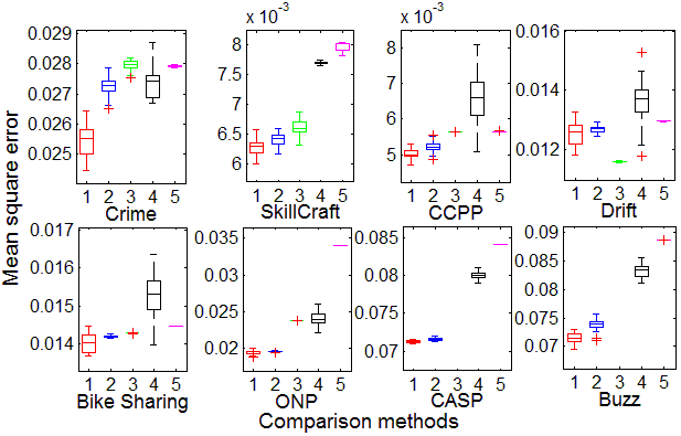
For large-scale datasets, Figure 2 and Table 2 summarize the results for the linear kernel. As one can see, e-DWSVR performs better than other regression methods on some datasets, and it always performs better than e-SVR. In addition, linear regression did not return the results on some datasets after 48 hours (indicated as NA in Table 2).
|
e-DWSVR | e-SVR | LINEAR | NN | Logistic | ||
|---|---|---|---|---|---|---|---|
| Crime (1994 / 128) | 0.5613 | 0.5348 | 0.4430 | 0.5244 | 0.5350 | ||
| SkillCraft (3338 / 18) | 0.7275 | 0.7018 | 0.7013 | 0.6843 | 0.6147 | ||
| CCPP (9568 / 4) | 0.8634 | 0.8327 | 0.8246 | 0.7334 | 0.8286 | ||
| Drift (13910 / 129) | 0.5620 | 0.5636 | 0.5888 | 0.5490 | 0.5574 | ||
| Bike sharing (17389 / 16) | 0.5867 | 0.5825 | 0.5938 | 0.5395 | 0.5465 | ||
| ONP (39797 / 61) | 0.4598 | 0.4590 | 0.3856 | 0.3544 | 0.2113 | ||
| CASP (45730 / 9) | 0.2755 | 0.2608 | NA | 0.1836 | 0.1657 | ||
| Buzz (140000 / 77) | 0.2976 | 0.2591 | NA | 0.1529 | 0.1373 |
4.3 Time cost and parameter effect
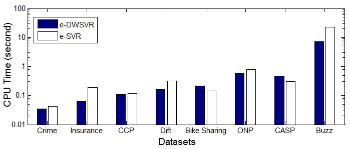
In Figure 3 we present a comparison of CPU time taken between e-SVR and e-DWSVR on each dataset. e-SVR for large-scale problems was implemented by the LIBLINEAR [17] package and e-DWSVR was implemented by ASGD. According to Figure 3, e-DWSVR cost less time than e-DWSVR on most datasets, and it is only slightly slower than e-SVR on two datasets.
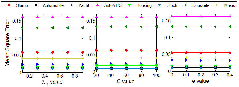
Furthermore, Figure 4 shows that the MSE on the medium-scale datasets does not have much difference with the change of the parameters. This indicates that the performance of e-DWSVR is not sensitive to the parameters, which shows the robustness of e-DWSVR.
5 Conclusion and future work
In this paper, we propose e-DWSVR, a novel and promising SVR algorithm. e-DWSVR overcomes the limitations of existing SVR systems and outperforms other regression methods on several benchmark datasets. We envision great application potential of e-DWSVR in various problems, including feature extraction, anomaly detection, and complex data interpretation. In the near future, we will apply e-DWSVR to solve several real-world problems, including bioinformatics anaysis and financial data prediction and anomaly detection.
6 Acknowledgement
We gratefully thank Dr Teng Zhang and Prof Zhi-Hua Zhou for providing the source code of “LDM” source code and their kind technical assistance. We also thank Prof Chih-Jen Lins team for providing the Libsvm and Liblinear packages and their support. This work is supported by the National Natural Science Foundation of China (Nos. 61472159, 61572227) and Development Project of Jilin Province of China (Nos.20140101180JC, 20160204022GX). This work is also partially supported by the 2015 Scottish Crucible Award funded by the Royal Society of Edinburgh and the 2016 PECE bursary provided by the Scottish Informatics & Computer Science Alliance (SICSA).
References
[1] V. Vapnik C. Cortes. Support vector machine. Machine Learning, 7(2002):1–28, 1995.
[2] J. D. Brown, M. F. Summers, and B. A. Johnson. Prediction of hydrogen and carbon chemical shifts from rna using database mining and support vector regression. Journal of Biomolecular Nmr, 63(1):1–14, 2015.
[3] C. Y. Deng and H. W. Lin. Progressive and iterative approximation for least squares b-spline curve and surface fitting. Computer-Aided Design, 47(1):32–44, 2014.
[4] M. V. Butz, G. K. M. Pedersen, and P. O. Stalph. Learning sensorimotor control structures with xcsf: redundancy exploitation and dynamic control. In Proceedings of the 11th Annual Conference on Genetic and Evolutionary Computation, pages 1171–1178, 2009.
[5] D. Liu, T.R. Li, and D. C. Liang. Incorporating logistic regression to decision-theoretic rough sets for classifications. International Journal of Approximate Reasoning, 54(1):197–210, 2014.
[6] K. Hagiwara, T. Hayasaka, N. Toda, S. Usui, and K. Kuno. Upper bound of the expected training error of neural network regression for a gaussian noise sequence. Neural Networks, 14(10):1419–1429, 2001.
[7] A. J. Smola and B. Scholkopf. A tutorial on support vector regression. Statistics and Computing, 14(3):199–222, 2004.
[8] B. Demir and L. Bruzzone. A multiple criteria active learning method for support vector regression. Pattern Recognition, 47(7):2558–2567, 2014.
[9] B Scholkopf, A. J. Smola, R. C. Williamson, and P. L. Bartlett. New support vector algorithms. Neural Computation, 12(5):1207–1245, 2000.
[10] B. Gu, V. S. Sheng, Z. J. Wang, D. Ho, S. Osman, and S. Li. Incremental learning for v-support vector regression. Neural Networks the Official Journal of the International Neural Network Society, 67(C):140– 150, 2015.
[11] J. S. Marron. Distance-weighted discrimination. Journal of the American Statistical Association, 102(12):1267–1271, 2007.
[12] X. Y. Qiao and L. S. Zhang. Distance-weighted support vector machine. Statistics and Its Interface, 8(3):331–345, 2013.
[13] T. Zhang and Z. H. Zhou. Large margin distribution machine. In Proceedings of the 20th ACM SIGKDD International Conference on Knowledge Discovery and Data Mining, pages 313–322, 2014.
[14] Z. H. Zhou. Large margin distribution learning. In Proceedings of the 6th Artificial Neural Networks in Pattern Recognition, pages 1–11, 2014.
[15] B. T. Polyak and A. B. Juditsky. Acceleration of stochastic approximation by averaging. Siam Journal on Control and Optimization, 30(4):838–855, 1992.
[16] T. Zhang. Solving large scale linear prediction problems using stochastic gradient descent algorithms. In Proceedings of the 21st International Conference on Machine Learning, pages 919–926, 2004.
[17] R. E. Fan, K. W. Chang, C. J. Hsieh, X. R. Wang, and C. J. Lin. Liblinear: A library for large linear classification. Journal of Machine Learning Research, 9(12):1871–1874, 2010.
[18] B. Scholkopf and A. Smola. Learning with kernels : support vector machines, regularization, optimization, and beyond. MIT Press, 2002.
[19] C. C. Chang and C. J. Lin. Libsvm: A library for support vector machines. Acm Transactions on Intelligent Systems and Technology, 2(3):389–396, 2011.
[20] G. X. Yuan, C. H. Ho, and C. J. Lin. Recent advances of large-scale linear classification. Proceedings of the IEEE, 100(9):2584–2603, 2012.
[21] Z. Q. Luo and P. Tseng. On the convergence of the coordinate descent method for convex differentiable minimization. Journal of Optimization Theory and Applications, 72(1):7–35, 1991.
[22] L. Bottou. Large-Scale Machine Learning with Stochastic Gradient Descent. Physica-Verlag HD, 2010.
[23] W. Xu. Towards optimal one pass large scale learning with averaged stochastic gradient descent. Computer Science, 2011.
[24] M. Lichman. UCI machine learning repository. http://archive.ics.uci.edu/ml, 2013.
[25] D. N. Guo, S. Shamai, and S. Verdu. Mutual information and minimum mean-square error in gaussian channels. IEEE Transactions on Information Theory, 51(4):1261–1282, 2005.
[26] W. Wen, R. Luo, X. J. Tang, L. Tang, H. X. Huang, X. Y. Wen, S. Hu, and B. Peng. Age-related progression of arterial stiffness and its elevated positive association with blood pressure in healthy people. Atherosclerosis, 238(1):147–152, 2015.