Optimal resampling for the noisy OneMax problem
Abstract
The OneMax problem is a standard benchmark optimisation problem for a binary search space. Recent work on applying a Bandit-Based Random Mutation Hill-Climbing algorithm to the noisy OneMax problem showed that it is important to choose a good value for the resampling number to make a careful trade off between taking more samples in order to reduce noise, and taking fewer samples to reduce the total computational cost. This paper extends that observation by deriving an analytical expression for the running time of the Random Mutation Hill-Climbing algorithm with resampling applied to the noisy OneMax problem, and showing both theoretically and empirically that the optimal resampling number increases with the number of dimensions in the search space.
Index Terms:
Noisy OneMax, resampling, Random Mutation Hill-Climber (RMHC)I Introduction
Evolutionary Algorithms (EA) have been widely used in both continuous and discrete domains [1, 2, 3].
Resampling111In this paper, “resampling” refers to the multiple re-evalutions of a solution. has proved to be a powerful tool in improving the local performance of EAs in noisy optimisation [3, 4, 5], and different resampling rules have been applied to a variety of EAs in continuous noisy optimisation, as studied in [6, 7]. Akimoto et al. [8] concluded that the running time for an adapted algorithm using resampling to solve a problem with additive Gaussian noise is similar to the runtime in the noise-free case when multiplying by a factor , where is the problem dimension.
Previous work on solving the OneMax problem [9] has concentrated on using a (1+1)-Evolution Algorithm (EA) [10, 11]. The OneMax problem with One-bit noise (exactly one uniformly selected bit changes with probability due to the noise) has been studied previously by Droste [10]. Qian et al. [11] claimed that resampling wasn’t beneficial in optimising OneMax with additive Gaussian noise using (1+1)-EA. Recently, Liu et al. [12, 13] applied a bandit-based RMHC to the noisy OneMax problem, and showed that it was important to choose an optimal resampling number, so as to compromise the reduction in sampling noise against the cost of doing so.
The main contribution of this work is the analysis of the optimal resampling number in the OneMax problem, in the presence of additive Gaussian noise. We show that the optimal resampling number increases with the problem dimension.
The paper is structured as follows. Section II provides a brief review of the related work and describes our noisy OneMax problem. Section III explains the modified Random Mutation Hill-Climbing algorithm used in the noisy context. Section IV analyses the optimal resampling number in the defined noisy OneMax problem. Experimental results are presented and discussed in Section V. Finally, Section VI concludes the work.
II Background
This section is organised as follows. Section II-A presents the original Random Mutation Hill-Climbing algorithm and its relation to (1+1)-EA. Section II-B recalls the OneMax problem, then a noisy variant of OneMax problem is defined in Section II-C. More related literatures in solving different noisy variants of OneMax problems are discussed in Section II-D
II-A Random Mutation Hill-Climbing
The Random Mutation Hill-Climbing (RMHC), also called Stochastic Hill Climbing, is a derivative-free optimisation method mostly used in discrete domains [14, 15]. RMHC can also be seen as an evolutionary algorithm in which there is a population of just one individual, and at each generation a child genome is formed from the current (best-so-far) individual by mutating exactly one gene, chosen uniformly at random. After mutation, the mutated child genome replaces its parent if its fitness value is improved or equivalent. In other words, RMHC randomly selects a neighbour candidate in the search space (where neighbour means it differs in exactly one gene) and updates its current candidate using a fitness-comparison-based method.
Borisovsky and Eremeev [16] proved that under some conditions, RMHC outperforms other EAs in terms of the probability of finding an anytime solution on several problems including OneMax.
(1+1)-EA is a variant of RMHC, the only difference being that every gene of the current individual’s genome mutates with a certain probability at each generation.222However note that some communities refer to RMHC as “(1+1)-Evolutionary Algorithm (EA)”, but we will avoid that description. (1+1)-EA has been widely used in both discrete and continuous optimisation problems [16]. A variant of (1+1)-EA is the closely related “(1+1)-Evolutionary Strategy (ES)” [17], which uses a self-adaptive mutation step-size and is applicable to real-valued search spaces.
Despite its simplicity, RMHC often competes surprisingly well with more complex algorithms [18], especially when deployed with random restarts. For instance, Lucas and Reynolds evolved Deterministic Finite Automata (DFA) [14, 15] using a multi-start RMHC algorithm with very competitive results, outperforming more complex evolutionary algorithms, and for some classes of problems also outperforming the state of the art Evidence-Driven State Merging (EDSM) [19] algorithms.
II-B OneMax problem
The OneMax problem [9] is a standard benchmark optimisation problem for a binary search space and has been deeply studied in the previous literatures [2, 20, 21]. The objective is to maximise the number of s occurring in a binary string, i.e., for a given -bit string , the fitness function to maximise for that string is given by
| (1) |
where denotes the bit in the string , and is either 1 or 0.
II-C Noisy OneMax
In this work, we study a noisy variant of the OneMax problem, where the fitness function is corrupted by some additive unbiased normally distributed noise with constant variance, formalised in (2).
| (2) |
with denoting a Gaussian noise, with mean and variance . From now on, we will use to denote the call to noisy fitness function on . At each call, the noise is independently sampled from and takes effect after the true fitness is evaluated.
There is a variety of noise models for the OneMax problem, as described in the next section. To avoid confusion, the term “noisy OneMax” refers to (2), the noisy variant used in this paper. Also, the “noisy” refers to the noise in the fitness function’s ability to read the true fitness of the genome; not the mutations which are deliberately applied to the genome, which could be interpreted as a second kind of “noise”.
II-D Related work
Different noise models for the OneMax problem have been studied before.
Proportionate selection is noise invariant
Our noise model is the same as the one used in [22]. Miller and Goldberg [22] used a GA with parents and offsprings, and proved that increasing noise level did not affect selection pressure for Genetic Algorithms (GA) using fitness-proportionate selection, in which each individual survives with a probability proportional to its fitness divided by the average fitness in the population [22, 23].
Resampling does not add benefit in low dimension
Qian et al. [11] applied (1+1)-EA using mutation probability and at most resamplings to a -bit noisy OneMax problem corrupted by additive Gaussian noise with variance ((2) with ), and concluded that resampling wasn’t beneficial for the (1+1)-EA in optimising the noisy OneMax problem. In their model, resampling had the effect of lowering the variance of the noise to , which is exactly as big as the lower bound of the differences between distinct noise-free fitness values. With that level of resampling and problem dimension, the problem is still difficult to solve. We present, later in this paper, our application of RMHC using larger resampling numbers in noisy OneMax, with noise variance and do observe that resampling adds a significant benefit when the dimension is above (Section V).
Solving high dimension noisy OneMax
Sastry et al. [24] designed a fully parallelised, highly-efficient compact Genetic Algorithm (cGA) to solve very high dimension problems, and compared it to RMHC on a noisy OneMax problem using noise variance depending linearly on the length of string, to allow for more difficult problems, for the reason that a randomly initiated -bit string has fitness variance . RMHC without resampling performed poorly when the problem dimension is higher than .
Noise takes effect before the evaluation
Droste [10] defined a One-bit noise model for the OneMax problem, in which during every fitness evaluation of the bit-string , there was exactly one uniformly-chosen random bit mis-read with probability . Hence the measured noisy fitness values are equivalent to replacing the Gaussian noise term in (2) by an appropriate discrete random variable taking values from . Under this scheme, Droste showed that (1+1)-EA with mutation probability could optimise a -bit OneMax problem corrupted by One-bit noise, with high probability, in polynomial time if is .
III Random Mutation Hill-Climbing in noisy context
When RMHC is applied to the noisy OneMax fitness function (2), a mutation of the gene refers to flipping the bit of the string. The standard deviation of the second term in (2) (the explicit noise term) is of the same order of magnitude as the noise in the first term of (2) (the OneMax fitness term) introduced by mutations from the RMHC algorithm. This extremely poor signal-to-noise ratio would cause major problems for hill-climbing strategies such as RMHC. Hence, we use RMHC with resampling, applied to the noisy OneMax problem, so as to try to reduce the unwanted variance, and to allow the hill climber to work.
III-A Noise-free case
Algorithm 1 recalls the generic RMHC, without any resampling. This is suitable for noise-free problems.
Here we have assumed the fitness value of the best-so-far genome could be stored after each cycle. If, alternatively, no space was allocated to store that fitness value, or if fitness evaluations can only be made by directly comparing two individuals, then the best-so-far genome’s fitness would need to be re-evaluated at each generation, thus raising the algorithm’s “evaluation count”, , by a factor of approximately 2.
.
III-B Noisy case
The previous RMHC algorithm (Algorithm 1) was applicable to deterministic fitness functions. Algorithm 2 extends this RMHC algorithm to be applicable to noisy fitness functions. It achieves this extension by using resampling, so that each genome is evaluated multiple times, so as to reduce the effect of noise which might interfere with hill climbing.
Additionally, if the statistics of the best-so-far genome can be stored, instead of comparing directly the fitness values of the offspring to the fitness of the parent (the best-so-far genome), the average fitness value of the best-so-far genome in the history is compared at each generation (line 11 of Algorithm 2).
IV Analysis of optimal resampling number in noisy OneMax problem
This section analyses the application of the modified RMHC algorithm (Algorithm 2) to the noisy OneMax problem, with fixed noise level, by describing it as a Markov process. Several variants of Algorithm 2 are considered in Section IV-B, including analysis of varying the resampling number, and of the effect of storing a statistic of the best-so-far genome versus not storing it. The benefit of storing the statistics of the best-so-far genome is illustrated in Section IV-B. Section IV-C derives an expression for the length of Markov chain that represents the learning algorithm, and the optimal level of resampling is calculated and displayed, in Section IV-D.
We restrict the analysis in this section to a fixed noise level . This noise level is a significant challenge for RMHC, as the difference between the parent’s fitness and the one of the offspring is always in our model. This motivates resampling, since resampling a candidate solution times can reduce the variance of the noise by a factor of . The extension of this analysis to the general would be straightforward.
IV-A Markov chain description for noisy OneMax
We consider a -bit OneMax problem with constant variance Gaussian noise, . Throughout this section, we summarise the n-bit OneMax state vector by a single scalar number, , equal to the number of ones in the n-bit string. As the RMHC algorithm makes mutations to the full bit string, the compressed state-representation, , will change by . The transition probabilities for the change in are dependent only on the scalar . Hence the evolution of the variable is modeled by a Markov process.
After each mutation is initially made by the RMHC algorithm, the fitness of that mutated bit string is evaluated using (2), and the RMHC algorithm will either accept or reject that mutation.
Let , , and denote the probability of true acceptance, false acceptance, true rejection and false rejection, respectively, for the RMHC algorithm to accept or reject any given mutation. These four probabilities depend on the resampling strategy employed by the RMHC algorithm, and are derived in Section IV-B. However, since complementary probability pairs must sum to one, we do generally have that,
| (3) | |||||
| (4) |
Assuming these acceptance and rejection probabilities are known, we can then derive the Markov state transition probabilities as follows:
For any state scalar , the corresponding OneMax bit string has ones and zeros. Therefore the probability of uniformly randomly choosing a zero bit is . Hence, for RMHC to make an improvement to the genome, it must randomly choose one of these zero bits and that mutation must be accepted. Therefore the transition probability from state to state in one generation is:
| (5) |
Similarly, for RMHC to make the genome worse, it must choose a one bit (with probability ) and flip it to a zero, and that mutation must be accepted, with probability . Hence we obtain
| (6) |
For an RMHC mutation to make no progress in the genome, the mutation must be rejected. This could mean a one bit is chosen (with probability ) and rejected (with probability ), or it could be that a zero bit is chosen (with probability ) and rejected (with probability ). Hence we obtain
| (7) |
The probabilities given by (5)-(7) appear on the three arrows emanating from the central node “” in the Markov chain shown in Figure1. The Markov chain’s absorption state is state , since the OneMax problem is solved and terminates as soon as is reached.

IV-B Rejection and acceptance probabilities for noisy OneMax problem with RMHC
The Markov Process described in the previous subsection relied upon knowledge of the acceptance and rejection probabilities and , which are dependent on the RMHC resampling method chosen.
We discuss three RMHC resampling cases here, and calculate the corresponding acceptance/rejection probabilities. We consider three separate cases:
IV-B1 No resampling, no statistic of the best-so-far genome is stored
If no statistic of the best-so-far genome is stored, the best-so-far one needs to be re-evaluated once at each generation in the case without resampling.
First we assume that the newly generated genome is better than the current genome , i.e. , where this fitness function is the noise-free version given by (1). Since is the true fitness of string , we have , the number of ones in string . Since the two genomes and are evaluated using the noisy fitness function (2), and since we are comparing and without resampling or storing the statistics of the best-so-far genome, the probability of true acceptance is
where and are independent samples from , thus . Then,
| (8) | |||||
Respectively, if the newly generated genome is worse than the current genome , i.e. , when comparing two genomes without resampling or storing the statistics of the best-so-far genome, the probability of true rejection is
| (9) | |||||
IV-B2 When comparing two genomes using resamplings without storing the statistics of the best-so-far genome
If each genome can be re-evaluated times, i.e., resamplings are used, but still no statistic of the best-so-far genome is stored, and are compared at each generation (lines 8 and 9 of Algorithm 2). Therefore, the variance of and , given and , are . Then,
where and are independent samples from , thus . Then,
| (10) | |||||
Similarly, holds in this case.
The probability of transferring from state to state in one generation is , larger than the probability in the previous case without resampling (Section IV-B1).
Therefore, the probability of true acceptance is improved by resampling genomes.
IV-B3 When comparing two genomes using resamplings and the statistics of the best-so-far genome
Additionally, if one has access to , the average fitness value of the best-so-far genome, and , the number of times that the best-so-far genome has been evaluated, by line 11 of Algorithm 2
| (11) |
with . Therefore, the variance of , given , is . The variance of , given , is .
The probability of true acceptance is
where and are independent samples from and , respectively. Thus, . Then,
| (12) | |||||
Similarly, holds in this case.
The probability of transferring from state to state in one generation is with , larger than the probabilities in the previous cases (Sections IV-B1 and IV-B2).
Therefore, the probability of true acceptance is improved by resampling genomes and storing the statistics of the best-so-far genome. However, the trade-off between the total evaluations and the accuracy needs to be considered.
IV-C Markov chain analysis
Now that we have described the Markov chain in Section IV-A, and derived the acceptance and rejection probabilities for the noisy OneMax problem in Section IV-B, we next derive an analytical expectation for the full trajectory length for solving the noisy OneMax problem, using RMHC with resamplings, starting from a bit string full of zeros. To simplify analysis, no stored statistic is considered (), thus we consider the second case discussed previously in Section IV-B2.
The Markov chain length can be found by defining the notation to mean the expectation of the number of generations required to get from a Markov state with value to a Markov state with value .
By considering the three arrows that emanate from the central node in Figure1, we can form an algebraic expression for , as follows:
| (13) |
The three terms in (13) correspond to the three arrows from node in Figure1, pointing to nodes , and , respectively.
Since it is always necessary to go from state to via their middle state , we can form the relationship
Furthermore, reusing (3) and (4), i.e. , , together with from Section IV-B, we get:
| (14) | |||||
Solving 14 for , which appears three times in that equation, we get:
| (15) |
This is a recursive equation that defines the term in terms of the term. To terminate this recursion, an explicit expression for can be found by considering the number of generations required to get from (i.e. a string with all zeros in it) to (i.e. a string with exactly one 1 in it). This is given by
| (16) |
(15) and (16) form a recursion that easily can be unrolled computationally, and it gives us the exact theoretical number of transitions to traverse from one Markov state to the adjacent Markov state . Therefore to calculate the total number of generations required to solve the noisy OneMax problem from an initial Markov state , we need to calculate . This can be expanded by adding all of the intermediate state transitions to get
| (17) |
(17) completes the theoretical analysis of the number of steps required by RMHC to solve the noisy OneMax problem, from an initial bit string of zeros. Note that each term of this sum needs a solution to the recursive equations given by (15) and (16), but with careful caching, the whole sum can be evaluated in steps.
It’s notable that even though the above Markov chain analysis was aimed at Case 2 (Section IV-B2, i.e. with resampling and no statistic stored), it also holds when there is no resampling, i.e., (the first case detailed in Section IV-B1). In both cases, is deterministic given the resampling number . However, Case 3 (Section IV-B3) is not as straightforward to analyse, because in that case that the average fitness value () depends on the evaluation number (), and is stochastic. Hence, (12) changes at each generation of RMHC. Case 3 has not been analysed in this paper, but it would be interesting to do so in the future.
IV-D Analytical results of RMHC in noisy OneMax problem
At each generation of the actual RMHC algorithm, fitness-function evaluations are required, so that the total number of fitness evaluations required to solve the noisy OneMax problem is
| (18) |
This result is shown graphically in Figure2, with various number of resamplings () and problem dimension (), under the assumption that no statistic is stored for the fitness of the best-so-far genome (case 2 described in Section IV-B2).
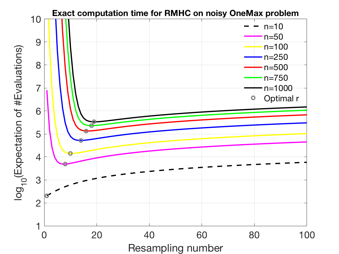
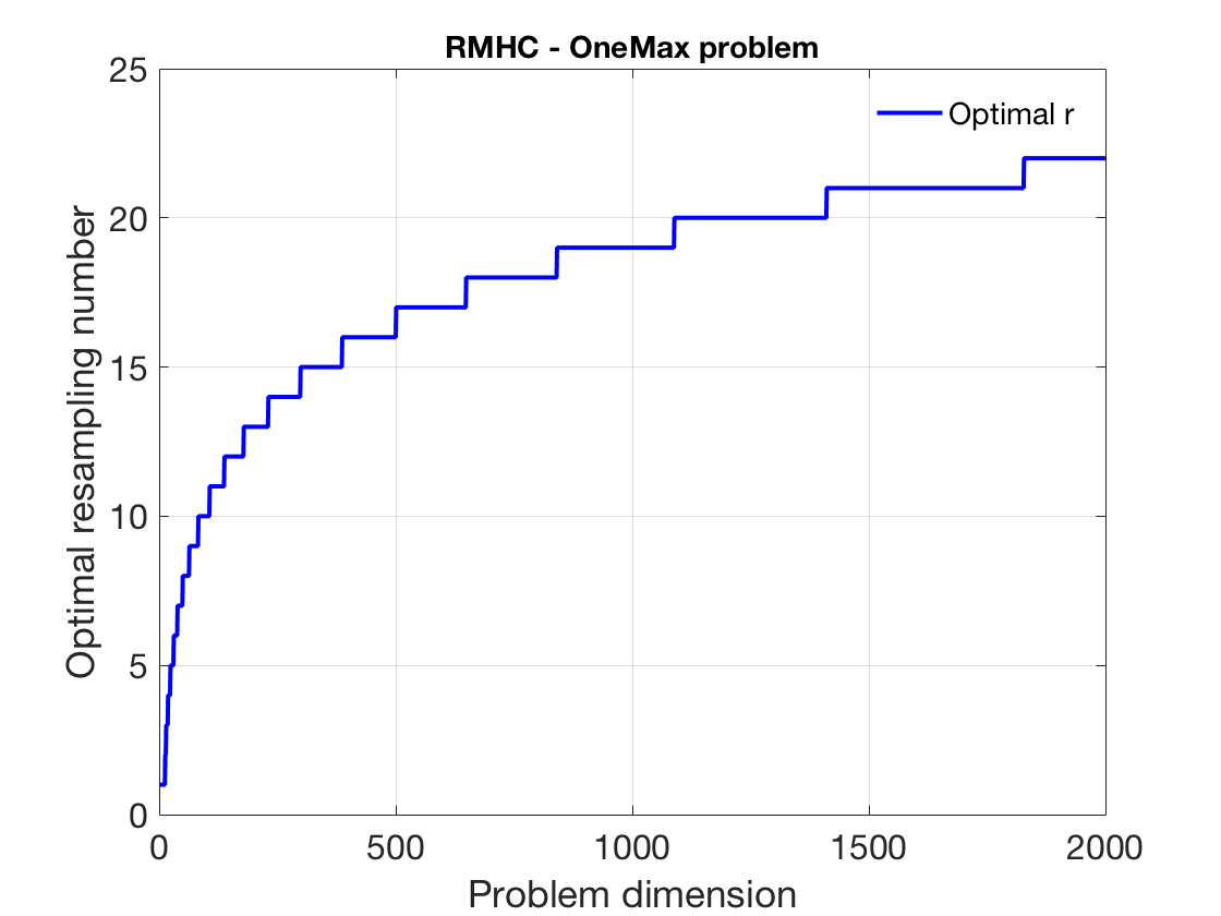
As can be seen from the location of the minima in Figure2, indicated by the small grey circles, the optimal resampling number increases with the problem dimension. The exact optimal number of resamplings to make in different dimensions is displayed in Figure3.
V Experimental results
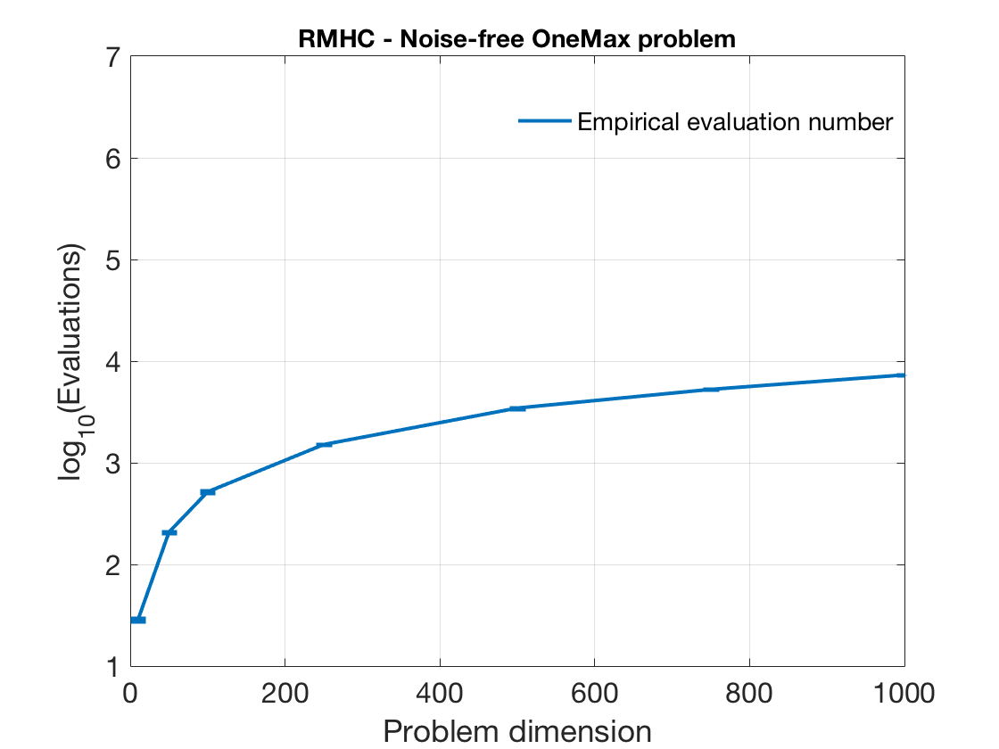
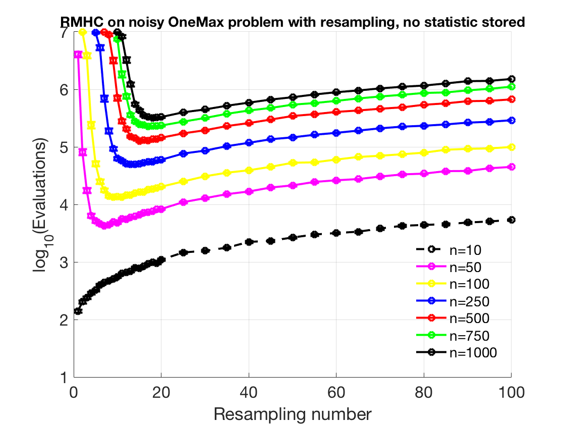
To supplement the theoretical results of the previous and to prove the benefit of storing statistics of the best-so-far genome at each generation, we apply first RMHC on the OneMax problem in a noise-free case (Figure4), then evaluate the performance of RMHC on the OneMax problem with the presence of constant variance Gaussian noise (Figure5). Each experiment was repeated times, initialised by an all zeros string. The following may be observed from the figures:
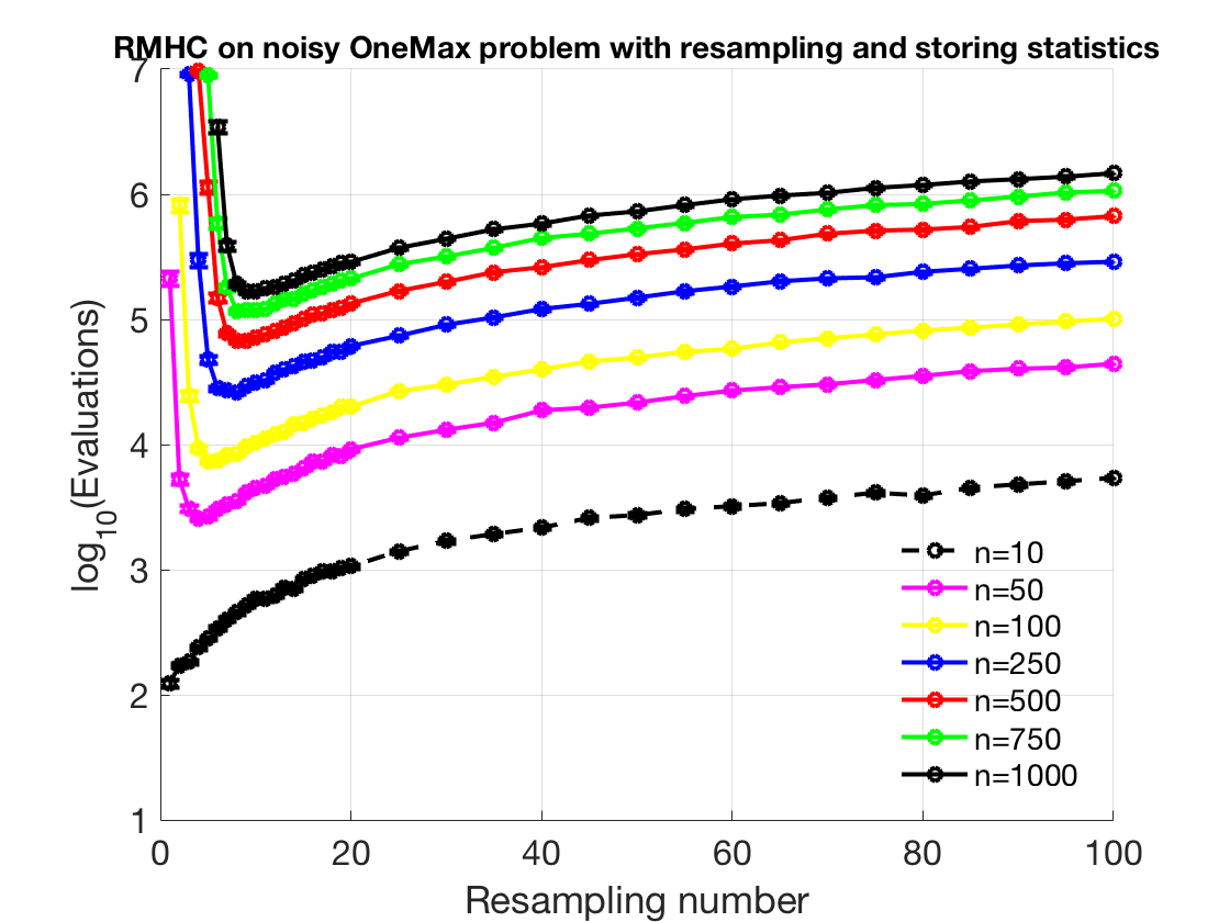
-
•
due to the noise, far more fitness evaluations are required to find the optimum in the noisy case than in the noise-free context;
-
•
the higher dimension problem required more fitness evaluations to reach the optimum;
-
•
in dimensions 10, no resampling leads to a reduction in the number of required fitness evaluations;
-
•
in higher dimensions (), the optimal amount of resampling required increases with the problem dimension;
-
•
in higher dimensions (), the evaluation number is significantly reduced by using the stored statistic.
Additionally, Figure5 clearly shows the benefit of storing the average fitness value and the current evaluation number of the best-so-far genome at the end of each generation (case 3 described in Section IV-B3).
V-A Validation of Theoretical results
To validate the theoretical results and equations of Section IV, Table I demonstrates a very close match between the theoretically obtained number of evaluations (derived from (15)-(18)) and the equivalent empirically calculated numbers (i.e. those found by actually running the RMHC algorithm repeatedly and averaging). This table hopefully validates the accuracy of our theoretical derivations and our numerical implementation.
| Expected #evaluations | Empirical #evaluations | |
|---|---|---|
| 1 | 205.8283 | 205.1998 |
| 2 | 238.5264 | 239.7504 |
| 3 | 276.3340 | 274.9920 |
| 4 | 317.9576 | 317.8848 |
| 5 | 362.4065 | 363.2520 |
| 10 | 612.2250 | 611.0060 |
VI Conclusion
This paper presents a noisy OneMax problem with additive constant variance Gaussian noise and analyses the optimal resampling number required by the Random Mutation Hill Climber (RMHC) to handle the noise.
The number of fitness evaluations required by RMHC to find the optimal solution in the noisy OneMax problem varies with the resampling number. In a very low-dimensional noisy OneMax problem (dimension 10, hence the string only has possible values), the optimal value may be found by a random walk, and resampling can be counterproductive in these cases (it leads to the remarkable growth of the number of evaluations required to find the optimum as shown in Figure5). However, in higher dimensions, resampling to reduce the noise is of critical importance, and makes the difference between success and failure. The optimal level of resampling increases with the dimension in the search space (as shown empirically in Figure2, and analytically in Figure3). This is an interesting result, which for this particular benchmark problem, is in conflict with the observation by Qian et al. in [11] that resampling was not beneficial.
RMHC is simple but efficient. The success of (-)-GA, of which (1+1)-EA can be seen as a variant, depends on one or more parameters, such as the size of the population, , the number of parents, , and the crossover and mutation operators. RMHC does not have such details to adjust and is therefore simpler to apply. Due to its efficiency and simplicity RMHC should be considered as a useful tool for expensive optimisation tasks.
References
- [1] H. Muhlenbein, “How genetic algorithms really work: I. mutation and hill climbing. parallel problem solving from nature 2. b. manderick,” 1992.
- [2] S. Droste, T. Jansen, and I. Wegener, “On the analysis of the (1+1) evolutionary algorithm,” Theoretical Computer Science, vol. 276, no. 1, pp. 51–81, 2002.
- [3] D. V. Arnold and H.-G. Beyer, “A general noise model and its effects on evolution strategy performance,” Evolutionary Computation, IEEE Transactions on, vol. 10, no. 4, pp. 380–391, 2006.
- [4] H.-G. Beyer, The Theory of Evolution Strategies. Springer Science & Business Media, 2013.
- [5] S. Astete-Morales, M.-L. Cauwet, J. Liu, and O. Teytaud, “Simple and cumulative regret for continuous noisy optimization,” Theoretical Computer Science, vol. 617, pp. 12–27, 2016.
- [6] S. Astete-Morales, J. Liu, and O. Teytaud, “Log-log convergence for noisy optimization,” in International Conference on Artificial Evolution (Evolution Artificielle). Springer, 2013, pp. 16–28.
- [7] J. Liu, “Portfolio methods in uncertain contexts,” Ph.D. dissertation, INRIA, 12 2015.
- [8] Y. Akimoto, S. Astete-Morales, and O. Teytaud, “Analysis of runtime of optimization algorithms for noisy functions over discrete codomains,” Theoretical Computer Science, vol. 605, pp. 42–50, 2015.
- [9] J. D. Schaffer and L. J. Eshelman, “On crossover as an evolutionarily viable strategy,” in ICGA, vol. 91, 1991, pp. 61–68.
- [10] S. Droste, “Analysis of the (1+1) EA for a noisy OneMax,” in Genetic and Evolutionary Computation–GECCO 2004. Springer, 2004, pp. 1088–1099.
- [11] C. Qian, Y. Yu, Y. Jin, and Z.-H. Zhou, “On the Effectiveness of Sampling for Evolutionary Optimization in Noisy Environments,” in Parallel Problem Solving from Nature–PPSN XIII. Springer, 2014, pp. 302–311.
- [12] J. Liu, D. Peŕez-Liebana, and S. M. Lucas, “Bandit-based random mutation hill-climbing,” arXiv preprint arXiv:1606.06041, 2016. [Online]. Available: http://arxiv.org/abs/1606.06041
- [13] ——, “Bandit-based random mutation hill-climbing,” 2017 IEEE Congress on Evolutionary Computation (IEEE CEC), 2017.
- [14] S. M. Lucas and T. J. Reynolds, “Learning DFA: Evolution versus Evidence Driven State Merging,” in Evolutionary Computation, 2003. CEC’03. The 2003 Congress on, vol. 1. IEEE, 2003, pp. 351–358.
- [15] ——, “Learning deterministic finite automata with a smart state labeling evolutionary algorithm,” Pattern Analysis and Machine Intelligence, IEEE Transactions on, vol. 27, no. 7, pp. 1063–1074, 2005.
- [16] P. A. Borisovsky and A. V. Eremeev, “Comparing evolutionary algorithms to the (1+1)-EA,” Theoretical Computer Science, vol. 403, no. 1, pp. 33–41, 2008.
- [17] H.-G. Beyer, “Toward a theory of evolution strategies: On the benefits of sex—the (/, ) theory,” Evol. Comput., vol. 3, no. 1, pp. 81–111, Mar. 1995. [Online]. Available: http://dx.doi.org/10.1162/evco.1995.3.1.81
- [18] M. Mitchell and J. H. Holland, When will a Genetic Algorithm Outperform Hill-Climbing? Morgan Kaufmann, 1993.
- [19] O. Cicchello and S. C. Kremer, “Beyond EDSM,” in International Colloquium on Grammatical Inference. Springer, 2002, pp. 37–48.
- [20] B. Doerr and C. Winzen, “Memory-restricted black-box complexity of OneMax,” Information Processing Letters, vol. 112, no. 1, pp. 32–34, 2012.
- [21] C. Doerr and J. Lengler, “OneMax in black-box models with several restrictions,” Algorithmica, pp. 1–31, 2016. [Online]. Available: http://dx.doi.org/10.1007/s00453-016-0168-1
- [22] B. L. Miller and D. E. Goldberg, “Genetic algorithms, selection schemes, and the varying effects of noise,” Evolutionary Computation, vol. 4, no. 2, pp. 113–131, 1996.
- [23] M. Mitchell, An introduction to genetic algorithms. MIT press, 1998.
- [24] K. Sastry, D. E. Goldberg, and X. Llora, “Towards billion-bit optimization via a parallel estimation of distribution algorithm,” in Proceedings of the 9th annual conference on Genetic and evolutionary computation. ACM, 2007, pp. 577–584.