Density Estimation Trees as fast non-parametric modelling tools

Abstract

A Density Estimation Tree (DET) is a decision trees trained on a multivariate dataset to estimate the underlying probability density function. While not competitive with kernel techniques in terms of accuracy, DETs are incredibly fast, embarrassingly parallel and relatively small when stored to disk. These properties make DETs appealing in the resource-expensive horizon of the LHC data analysis. Possible applications may include selection optimization, fast simulation and fast detector calibration. In this contribution I describe the algorithm and its implementation made available to the HEP community as a RooFit object. A set of applications under discussion within the LHCb Collaboration are also briefly illustrated.

1 Introduction

The fast increase of computing resources needed to analyse the data collected in modern hadron-collider experiments, and the lower cost of processing units with respect to storage, pushes High-Energy Physics (HEP) experiments to explore new techniques and technologies to move as much as possible of the data analysis at the time of the data acquisition (online) in order to select candidates to be stored on disk, with maximal, reasonably achievable, background rejection. Besides, research on multivariate algorithms, active both within and outside of the HEP community, is approaching the challenge of operating in distributed computing environments, which represents a further motivation for studies of new classes of algorithms.

Statistical inference of probability density functions underlying experimental datasets is common in High Energy Physics. Fitting is an example of parametric density estimation. When possible, defining a parametric form of the underlying distribution and choose the values for the parameters maximizing the likelihood is usually the best approach. In multivariate problems with a large number of variables and important correlation, however, fitting may become unpractical, and non-parametric density estimation becomes a valid, largely employed, solution.

In HEP, the most common non-parametric density estimation, beyond the histogram, is probably kernel density estimation [1], based on the sum of normalized kernel functions centered on each data-entry.

In this write-up, I discuss Density Estimation Trees, algorithms based on a multivariate, binary tree structure, oriented to non-parametric density estimation. Density Estimation Trees are less accurate than kernel density estimation, but much faster. Integrating Density Estimation Trees is also trivial and fast, making iterative search algorithms convenient. Finally, storing a Density Estimation Trees and propagate it through the computing nodes of a distributed system is relatively cheap, offering a reasonable solutions for compressing the statistical information of large datasets.

An implementation of the algorithm in ROOT/RooFit is available through CERN GitLab.

2 The algorithm

The idea of iteratively splitting a data sample, making the density estimation to coincide with the average density in each portion of the data space is not new. However, the technique had little room for applications in analyses of datasets up to a few thousands of entries described by small sets of correlated variables.

Recently, $kd$-trees [2] have been used to split large samples into sub-sets consisting of equal fractions of the data entries. The idea underlying $kd$-trees is the iterative splitting of the data-sample using as threshold the median of a given projection. While powerful to solve a vast range of problems, including notably nearest-neighbour searches, the lack of appropriateness of $kd$-trees to estimate probability densities is evident considering samples including multiple data-entries.

Ideally, the density estimation $\hat{f}(\mathbf{x})$ approximating the underlying density function $f(\mathbf{x})$ should minimize the quantity $\mathcal{R}=\int\big{(}\hat{f}(\mathbf{x})-f(\mathbf{x})\big{)}^{2}\mathrm{d}\mathbf{x}.$ It can be shown [3] that, exploiting the Monte Carlo approximation

$$\lim_{N\to+\infty}\frac{1}{N}\sum_{i=1}^{N}g(x_{i})=\int g(x)h(x)\mathrm{d}x\qquad\mbox{where }x_{1},x_{2},...,x_{N}\mbox{ distribute as }h(x),$$ (1)

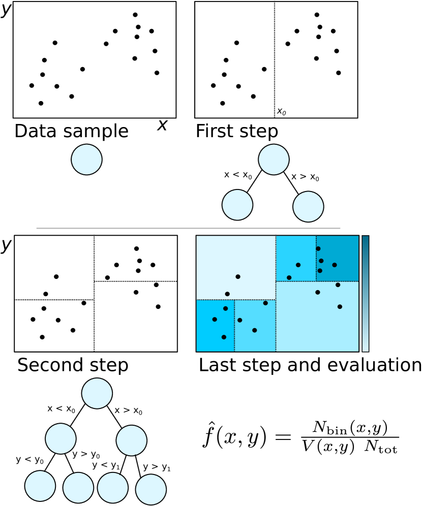
the minimization of $\mathcal{R}$ is equivalent to growing a Density Estimation Tree iteratively splitting the node $\ell$, into the two sub nodes $\ell_{R}$ and $\ell_{L}$ minimizing the Gini index, $G(\ell)=R(\ell)-R(\ell_{R})-R(\ell_{L})$. Here, $R(\ell)$ represents the replacement error, defined by

$$R(\ell)\equiv-\frac{N_{\ell}^{2}}{N^{2}_{\mathrm{tot}}V_{\ell}},$$ (2)

where $V_{\ell}$ is the hyper-volume of the portion of the data-space associated to the node $\ell$, and $N_{\ell}$ the number of data entries it includes; $N_{\mathrm{tot}}$ is the number of data entries in the whole dataset.

Figure 2 shows an example of how the training is performed.

Figure 1: Schematic representation of the training and the evaluation procedures of a Density Estimation Tree.

Figure 2: Top, an example of an overtrained Density Estimation Tree. The random alignment of data-entries with respect to one of the variables describing the problem is misinterpreted as a spike in the density estimation, as evident in the projection onto the vertical axis shown on the bottom.

2.1 Overtraining

As in the case of Classification algorithms, overtraining is the misinterpretation of statistical fluctuations of the dataset as relevant features to be reproduced by the model.

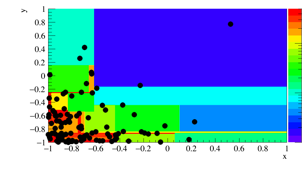
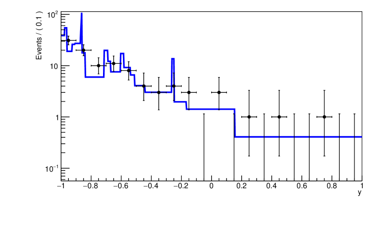
An example of overtraining of Density Estimation Trees is presented in Figure 2. In the presented dataset, the alignment of data-entries in one of the input variables is interpreted as narrow spikes. To compensate spikes, in terms of absolute normalization, the density is underestimated in all of the other points of the parameter space.

Overtraining in decision trees is controlled through an iterative approach consisting in pruning and cross-validation: finding and removing the branches increasing the complexity of the tree without enhancing the statistical agreement with a set of test samples. Cross-validation is very expensive in terms of computing power and often fails to identify problems of over-training arising close to the root of the decision tree.

Overtraining in density estimation is fought, instead, by defining a priori an expected resolution width, neglecting fluctuations under that resolution while building the statistical model. For example, kernel density estimation algorithms require a parameter, named bandwidth as an input. The bandwidth is related to the width of the kernel function. Abundant literature exists on techniques to optimise the bandwidth for a certain dataset, most of them represent a preliminary step of the density estimation algorithm. Growing a Density Estimation Tree with a minimal leaf width is fast, doesn’t require post-processing and it is found to result in better-quality estimations with respect to cross-validation procedures. The same techniques used to compute the optimal bandwidth parameter for kernel density estimation algorithms can be used to define the optimal minimal leaf width of the Density Estimation Tree.

2.2 Integration

As mentioned in the introduction, fast integration of the statistical model built using Density Estimation Trees is one of the strengths of the algorithm. Integration usually responds to two different needs: normalization and slicing (or projecting, or marginalizing).

Integrals to compute the overall normalization of the density estimation, or the contribution in a large fraction of the data-space, gain little from exploiting the tree structure of the density estimator. A sum over the contributions of each leaf represents the best strategy.

Instead, integrals over a narrow subset of the data-space should profit of the tree structure of the density estimation to exclude from the integration domain as many leaves as possible, as early as possible. Exploiting the tree structure when performing integrals of slices can drastically reduce the computing time in large density estimation trees.

2.3 Operations with Density Estimation Trees

Combining weighted Density Estimation Trees can be useful to model data samples composed of two or more components. Combination is achieved implementing both scalar and binary operations. There is not much to discuss about scalar operations, where the scalar operation is applied to each leaf independently. Instead, binary operations require the combination of two different Density Estimation Trees, which is not trivial because the boundaries are a priori different. The algorithm to combine two Density Estimation Trees consists of the iterative splitting of the terminal nodes of the first tree, following the boundaries of the terminal nodes of the second one. Once the combination is done, the first tree is compatible with the second one and the binary operation can be performed node per node. The resulting tree may have several additional layers with respect to the originating trees, therefore a final step removing division between negligibly different nodes is advisable.

3 Discussion of possible applications

Density Estimation Trees are useful to approach problems defined by many variables and for which huge statistical samples are available. To give a context to the following examples of applications, I consider the calibration samples for the Particle IDentification (PID) algorithms at the LHCb experiment.

PID calibration samples are sets of decay candidates reconstructed and selected relying on kinematic variables only, to distinguish between different types of long-lived particles: electrons, muons, pions, kaons, and protons.

The PID strategy of the LHCb detector relies on the combined response of several detectors: two ring Cherenkov detectors, an electromagnetic calorimeter, a hadronic calorimeter and a muon system [4]. The response of the single detectors are combined into likelihoods used at analysis level to define the tightness of the PID requirements.

Calibration samples count millions of background-subtracted candidates, each candidate is defined by a set of kinematic variables, for example momentum and pseudorapidity, and a set of PID likelihoods, one per particle type. The correlation between all variables is important and not always linear.

3.1 Efficiency tables

The first application considered is the construction of tables defining the probability that the PID likelihood of a candidate, defined by a set of kinematic variables, satisfies a particular requirement.

Building two Density Estimation Trees with the kinematic variables defining the data-space, one with the full data sample (tree $t_{\mathrm{all}}$), and one with the portion of data sample passing the PID criteria (tree $t_{\mathrm{pass}}$), allows to compute the efficiency for each combination of the kinematic variables by evaluating the Density Estimation Tree obtained taking the ratio $t_{\mathrm{pass}}/t_{\mathrm{all}}$.

For frequently-changing criteria a dynamic determination of the efficiency can be envisaged. For simplicity, consider the generic univariate PID criterion $y>0$. In this case a single Density Estimation Tree $d(x_{1},x_{2},y)$ defined by the kinematic variables $(x_{1},x_{2})$, and one PID variable $y$, has to be trained on the calibration sample. The dynamic representation of the efficiency for a candidate having kinematic variables $(\hat{x}_{1},\hat{x}_{2})$ is the ratio

$$\epsilon(x_{1},x_{2};y>0)={\displaystyle\int_{y>0}d(\hat{x}_{1},\hat{x}_{2},y)\mathrm{d}y}\Bigg{/}{\displaystyle\int_{\mathrm{any\ }y}d(\hat{x}_{1},\hat{x}_{2},y)\mathrm{d}y}.$$ (3)

Thanks to the fast slice-integration algorithm, the computation of this ratio can be included in an iterative optimization procedure aiming at an optimization of the threshold on $y$.

3.2 Sampling as fast simulation technique

Another important application is related to fast simulation of HEP events. Full simulation, including interaction of the particles with matter, is becoming so expensive to be expected exceeding the experiments’ budgets in the next few years. Parametric simulation is seen as a viable solution, as proved by the great interest raised by the DELPHES project [5]. However, parametrizing a simulation presents the same pitfalls as parametrizing a density estimation: when correlation among different variables becomes relevant, the mathematical form of the parametrization increases in complexity up to the point it becomes unmanageable.

Density Estimation Trees are an interesting candidate for non-parametric fast simulation. Let $d(x_{1},...,x_{N},y_{1},...,y_{n})$ be a Density Estimation Tree trained on a set of candidates defined by generator variables $\mathbf{x}\equiv(x_{1},...,x_{N})$, and by variables $\mathbf{y}\equiv(y_{1},...,y_{n})$ obtained through full simulation. For example, $\mathbf{x}$ could represent the kinematic variables of a track and $\mathbf{y}$ the PID likelihoods.

The aim of fast non-parametric simulation is, given a new set of values $(\hat{x}_{1},...,\hat{x}_{N})$ for $\mathbf{x}$, to compute a set of values for $\mathbf{y}$ distributed according to the conditional probability density function $d(y_{1},...,y_{n}|\hat{x}_{1},...,\hat{x}_{N})$.

Once the DET is trained, the tree structure of the density estimator is used to compute for each leaf $\ell$ the hyper-volume $V_{\ell\cap\hat{\mathbf{x}}}$ of the intersection between $\ell$ and hyper-plane defined by $\mathbf{x}=(\hat{x}_{1},...,\hat{x}_{N})$.

A random leaf $L\in\{\ell\}$ is then chosen with probability proportional to $V_{L\cap\hat{\mathbf{x}}}$, and variables $\mathbf{y}$ are generated following a flat distribution bounded within $L$.

A set of generator variables $\mathbf{x}$ can then be completed by the corresponding $\mathbf{y}$ variables without full simulation, but relying on the joint multivariate distribution learnt by the Density Estimation Tree.

4 Summary and outlook

I discussed Density Estimation Tree algorithms as fast modelling tools for high statistics problems characterized by a large number of correlated variables and for which an approximated model is acceptable. The fast training and integration capabilities make these algorithms of interest for the high-demanding future of the High-Energy Physics experiments. The examples discussed, which benefited from an active discussion within the Particle Identification Group of the LHCb collaboration, explore cases where the statistical features of huge samples have to be assessed in a time shorter than what standard estimators would require. In future, Density Estimation Trees could be sampled to train Regression Multivariate Algorithms, such as Neural Networks, in order to smooth the response and further speed up the query time, at the cost of loosing its fast-integration properties.

References

- [1] K. S. Cranmer, Comput. Phys. Commun. 136 (2001) 198 doi:10.1016/S0010-4655(00)00243-5 [hep-ex/0011057].
- [2] J. L. Bentley, Communications of the ACM 18 (1975) 9 doi:10.1016/S0010-4655(00)00243-5
- [3] P. Ram and A. G. Gray, Proceedings of the 17th ACM SIGKDD international conference on Knowledge discovery and data mining, pages 627-635
- [4] A. A. Alves et al., The LHCb detector at the LHC, JINST 3 (2008)
- [5] J. de Favereau et al. [DELPHES 3 Collaboration], JHEP 1402 (2014) 057 doi:10.1007/JHEP02(2014)057 [arXiv:1307.6346 [hep-ex]].