The Problem of Infra-marginality
in Outcome Tests for Discrimination

Abstract

Outcome tests are a popular method for detecting bias in lending, hiring, and policing decisions. These tests operate by comparing the success rate of decisions across groups. For example, if loans made to minority applicants are observed to be repaid more often than loans made to whites, it suggests that only exceptionally qualified minorities are granted loans, indicating discrimination. Outcome tests, however, are known to suffer from the problem of infra-marginality: even absent discrimination, the repayment rates for minority and white loan recipients might differ if the two groups have different risk distributions. Thus, at least in theory, outcome tests can fail to accurately detect discrimination. We develop a new statistical test of discrimination—the threshold test—that mitigates the problem of infra-marginality by jointly estimating decision thresholds and risk distributions. Applying our test to a dataset of 4.5 million police stops in North Carolina, we find that the problem of infra-marginality is more than a theoretical possibility, and can cause the outcome test to yield misleading results in practice.

Introduction

Claims of biased decision making are typically hard to rigorously assess, in large part because of well-known problems with the two most common statistical tests for discrimination. In the first test, termed benchmarking, one compares the rate at which whites and minorities are treated favorably. For example, in the case of lending decisions, if white applicants are granted loans more often than minority applicants, that may be the result of bias against minorities. However, if minorities in reality are less creditworthy than whites, then such disparities in lending rates may simply reflect reasonable business practices rather than discrimination. This limitation of benchmarking is referred to in the literature as the qualified pool or denominator problem (Ayres, 2002), and is a specific instance of omitted variable bias.

Ideally, one would like to compare similarly qualified white and minority applicants, but such a comparison requires detailed individual-level data and is often infeasible to carry out in practice. Addressing this shortcoming of benchmarking, Becker (1993, 1957) proposed the outcome test, which is based not on the rate at which decisions are made, but on the success rate of those decisions. Becker argued that even if minorities are less creditworthy than whites, minorities who are granted loans, absent discrimination, should still be found to repay their loans at the same rate as whites who are granted loans. If loans to minorities have a higher repayment rate than loans to whites, it suggests that lenders are applying a double standard, granting loans only to exceptionally qualified minorities. Though originally proposed in the context of lending decisions, outcome tests have gained popularity in a variety of domains, particularly policing (Goel et al., 2016, 2017; Ayres, 2002; Knowles et al., 2001). For example, when assessing bias in traffic stops, one can compare the rates at which searches of white and minority drivers turn up contraband. If searches of minorities yield contraband less often than searches of whites, it suggests that the bar for searching minorities is lower, indicative of discrimination.

Outcome tests, however, are imperfect barometers of bias. To see this, suppose that there are two, easily distinguishable types of white drivers: those who have a 1% chance of carrying contraband, and those who have a 75% chance. Similarly assume that black drivers have either a 1% or 50% chance of carrying contraband. If officers, in a race-neutral manner, search individuals who are at least 10% likely to be carrying contraband, then searches of whites will be successful 75% of the time whereas searches of blacks will be successful only 50% of the time. This simple example illustrates a subtle failure of outcome tests known as the problem of infra-marginality (Ayres, 2002), a phenomenon we discuss in detail below.

Our contribution in this paper is two-fold. First, we develop a new test for discrimination—the threshold test—that mitigates theoretical limitations of both benchmark and outcome analysis. Our test simultaneously estimates decision thresholds and risk distributions by fitting a hierarchical Bayesian latent variable model (Gelman et al., 2014). In developing this method, we clarify the statistical origins of the problem of infra-marginality. Second, we demonstrate that infra-marginality is more than a theoretical possibility, and can cause the outcome test to yield misleading results in practice. To do so, we analyze police vehicle searches in a dataset of 4.5 million traffic stops conducted by the 100 largest police departments in North Carolina.

Related work.

As the statistical literature on discrimination is extensive, we focus our review on policing. Benchmark analysis is the most common statistical method for assessing racial bias in police stops and searches. The key methodological challenge with this approach is estimating the race distribution of the at-risk, or benchmark, population. Traditional benchmarks include the residential population, licensed drivers, arrestees, and reported crime suspects (Engel and Calnon, 2004). Alpert et al. (2004) estimate the race distribution of drivers on the roadway by considering not-at-fault drivers involved in two-vehicle crashes. Others have looked at stops initiated by aerial patrols (McConnell and Scheidegger, 2001), and those based on radar and cameras (Lange et al., 2001), arguing that such stops are less prone to potential bias and thus more likely to reflect the true population of traffic violators. Studying police stops of pedestrians in New York City, Gelman et al. (2007) use a hierarchical Bayesian model to construct a benchmark based on neighborhood- and race-specific crime rates. Ridgeway (2006) studies post-stop police actions by creating benchmarks based on propensity scores, with minority and white drivers matched using demographics and the time, location, and purpose of the stops. Grogger and Ridgeway (2006) construct benchmarks by considering stops at night, when a “veil of darkness” masks race. Antonovics and Knight (2009) use officer-level demographics in a variation of the standard benchmark test: they argue that search rates that are higher when the officer’s race differs from that of the suspect is evidence of discrimination. Finally, “internal benchmarks” have been used to flag potentially biased officers by comparing each officer’s stop decisions to those made by others patrolling the same area at the same time (Ridgeway and MacDonald, 2009; Walker, 2003).

Given the inherent limitations of benchmark analysis, researchers have more recently turned to outcome tests to investigate claims of police discrimination. For example, Goel et al. (2016) use outcome analysis to test for racial bias in New York City’s stop-and-frisk policy. While outcome tests mitigate the problem of omitted variables faced by benchmark analysis, they suffer from their own limitations, most notably infra-marginality. The problem of infra-marginality in outcome tests was first discussed in detail by Ayres (2002), although previous studies of discrimination (Galster, 1993; Carr et al., 1993) indicate awareness of the issue. An early attempt to address the problem was presented by Knowles et al. (2001), who developed an economic model of behavior in which drivers balance their utility for carrying contraband with the risk of getting caught, while officers balance the utility of finding contraband with the cost of searching. Under equilibrium behavior, Knowles et al. argue that the hit rate (i.e., the search success rate) is identical to the search threshold, and so one can reliably detect discrimination with the standard outcome test. Engel and Tillyer (2008) note that the model of Knowles et al. requires strong assumptions, including that drivers and officers are rational actors, and that every driver has perfect knowledge of the likelihood that he will be searched. Anwar and Fang (2006) propose a hybrid test of discrimination that is based on the rankings of race-contingent search and hit rates as a function of officer race: if officers are not prejudiced, they argue, then these rankings should be independent of officer race. This approach circumvents the problems of omitted variables and infra-marginality in certain cases, but it cannot detect discrimination when officers of different races are similarly biased.

A New Test for Discrimination

A model of decision making

We begin by introducing a stylized model of decision making that is the basis of our statistical approach, and which also illustrates the problem of infra-marginality. We develop this framework in the context of police stops, though the model itself applies more generally.

During routine traffic stops, officers have latitude to search both driver and vehicle for drugs, weapons, and other contraband when they suspect more serious criminal activity. These decisions are based on a myriad of contextual factors visible to officers during stops, including a driver’s age and gender, criminal record, and behavioral indicators of nervousness of evasiveness. We assume that officers use this information to estimate the probability a driver is carrying contraband, and then conduct a search when that probability exceeds a fixed, race-specific search threshold $t_{r}$. Under this model, if officers have a lower threshold for searching blacks than whites (i.e., $t_{\text{black}}<t_{\text{white}}$), then we would say that black drivers are being discriminated against. Conversely, if $t_{\text{white}}<t_{\text{black}}$, we would say that white drivers are being discriminated against. And if the thresholds are approximately equal across race groups, we would say there is no discrimination in search decisions. In the economics literature, this is often referred to as taste-based discrimination (Becker, 1957). We treat both the probabilities and the search thresholds as latent, unobserved quantities, and our goal is to infer them from data.

(a)

(b)

Figure 1: Hypothetical signal distributions (solid curves) and search thresholds (dashed vertical lines) that illustrate how the benchmark and outcome tests can give misleading results.Under the model of Section 2.1, the search rate for a given group is equal to the area under the signal distribution above the threshold, and the hit rate is the mean of the distribution conditional on being above the threshold. Situations (a) and (b) are observationally equivalent: in both cases, red drivers are searched more often than blue drivers (71% vs. 64%), while searches of red drivers recover contraband less often than searches of blue drivers (39% vs. 44%). Thus, the outcome and benchmark tests suggest that red drivers are being discriminated against in both (a) and (b). This is true in (a), because red drivers face a lower search threshold than blue drivers. However, blue drivers are subject to the lower threshold in (b), contradicting the results of the benchmark and outcome tests.

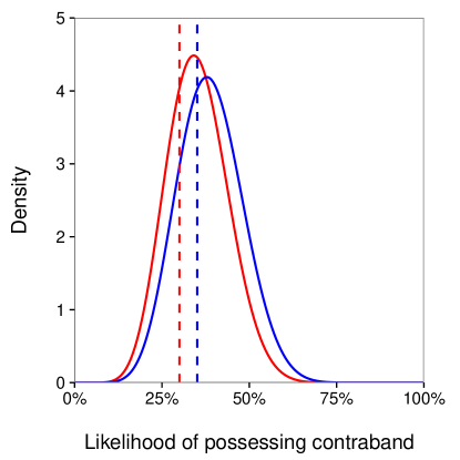
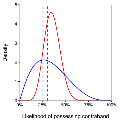
Fig. 1a illustrates the setup described above for two hypothetical race groups, where the curves show race-specific signal distributions (i.e., the distribution of guilt across all stopped motorists of that race), and the vertical lines indicate race-specific search thresholds. In this example, the red vertical line (at 30%) is to the left of the blue vertical line (at 35%), and so the red group, by definition, is being discriminated against. Under our model, the search rate for each race equals the area under the group’s signal distribution to the right of the corresponding race-specific threshold, which in this case is 71% for the red group and 64% for the blue group. The hit rate (i.e., the search success rate) for each race equals the mean of the group’s signal distribution conditional on being above the group’s search threshold, 39% for the red group and 44% for the blue group. The red group is thus searched at a higher rate (71% vs. 64%), and when searched, found to have contraband at a lower rate (39% vs. 44%) than the blue group. Both the benchmark test (comparing search rates) and the outcome test (comparing hit rates) correctly indicate that the red group is being discriminated against.

The problem of infra-marginality

To illustrate the problem of infra-marginality, Fig. 1b shows an alternative, hypothetical situation that is observationally equivalent to the one depicted in Fig. 1a, meaning that the search and hit rates of the red and blue groups are exactly the same in both settings. Accordingly, both the benchmark and outcome tests again suggest that the red group is being discriminated against. In this case, however, blue drivers face a lower search threshold (25%) than red drivers (30%), and therefore the true discrimination present is exactly the opposite of the discrimination suggested by the outcome and benchmark tests.

What went wrong in this latter example? It is easier in the blue group to distinguish between innocent and guilty individuals, as indicated by the signal distribution of the blue group having higher variance. Consequently, those who are searched in the blue group are more likely to be guilty than those who are searched in the red group, resulting in a higher hit rate for the blue group, throwing off the outcome test. Similarly, it is easier in the blue group to identify low-risk individuals, who need not be searched, in turn lowering the overall search rate of the group and leading to spurious results from the benchmark test. In this example, the search and hit rates are poor proxies for the search thresholds.

The key point about Fig. 1b is that it is not a pathological case; to the contrary, it seems quite ordinary, and a variety of mechanisms could lead to this situation. If innocent minorities anticipate being discriminated against, they might display the same behavior—nervousness and evasiveness—as guilty individuals, making it harder to distinguish those who are innocent from those who are guilty. Alternatively, one group may simply be more experienced at concealing criminal activity, again making it harder to distinguish guilty from innocent. Given that one cannot rule out the possibility of such signal distributions arising in real-world examples (and indeed we later show that such cases do occur in practice), the benchmark and outcome tests are at best partial indicators of discrimination. We address this so-called problem of infra-marginality by directly estimating the search thresholds themselves, instead of simply considering the search and hit rates.

Inferring search thresholds

We now describe our threshold test for discrimination, which mitigates the problem of infra-marginality in outcome tests. For each stop $i$, we assume that we observe: (1) the race of the driver, $r_{i}$; (2) the department of the officer, $d_{i}$; (3) whether the stop resulted in a search, indicated by $S_{i}\in\{0,1\}$; and (4) whether the stop resulted in a “hit” (i.e., a successful search), indicated by $H_{i}\in\{0,1\}$. Since a hit, by definition, can only occur if there was a search, $H_{i}\leq S_{i}$. Given a fixed set of stops annotated with the driver’s race and the officer’s department, we assume $S_{i}$ and $H_{i}$ are random outcomes resulting from a parametric process of search and discovery that formalizes the model of Section 2.1, described in detail below. Our primary goal is to infer race-specific search thresholds for each department. We interpret lower search thresholds for one group relative to another as evidence of discrimination. For example, if we were to find black drivers face a lower search threshold than white drivers, we would say blacks are being discriminated against.

We formalize this statistical problem in terms of a hierarchical Bayesian latent variable model. Our choice has two key benefits over natural alternatives. First, in contrast to maximum likelihood estimation, Bayesian inference automatically yields robust estimates of uncertainty (Gelman et al., 2014), obviating the need for bootstrapping, which can be computationally expensive for complex models such as ours. Second, hierarchical structure allows efficient pooling of evidence across departments. For example, if one race group is stopped only rarely in a given department, a hierarchical model can appropriately regularize department-level parameters toward state-level averages.

We next detail the generative model that underlies the threshold test. Consider a single stop of a motorist of race $r$ conducted by an officer in department $d$. Upon stopping the driver, the officer assesses all the available evidence and concludes the driver has probability $p$ of possessing contraband. Even though officers may make these judgements deterministically, there is uncertainty in who is pulled over in any given stop. We thus model $p$ as a random draw from a race- and department-specific signal distribution, which captures heterogeneity across stopped drivers. This formulation sidesteps the omitted variables problem of benchmark tests by allowing us to express information from all unobserved covariates as variation in the signal distribution. We can, in other words, think of the signal distribution as the marginal distribution over all unobserved variables.

We assume the signal $p$ is drawn from a beta distribution parameterized by its mean $\phi_{rd}$ (where $0<\phi_{rd}<1)$ and total count parameter $\lambda_{rd}$ (where $\lambda_{rd}>0$). The $\phi_{rd}$ term is the overall probability that a stopped driver of race $r$ in department $d$ has contraband, while $\lambda_{rd}$ characterizes the heterogeneity across stopped drivers of that race in that department. Turning to the search thresholds, we assume that officers in a department apply the same threshold $t_{rd}$ to all drivers of a given race, but we allow these thresholds to vary by driver race and by department. Given the randomly drawn signal $p$, we assume officers deterministically decide to search a motorist if and only if $p$ exceeds $t_{rd}$; and if a search is conducted, we assume that contraband is found with probability $p$.

As shown in Fig. 1, different $(\phi_{rd},\lambda_{rd},t_{rd})$ tuples can result in the same observed search and hit rates. Thus, we require more structure in the parameters to ensure they are identified by the data. To this end, we assume $\phi_{rd}$ and $\lambda_{rd}$ are functions of parameters that depend only on a motorist’s race ($\phi_{r}$ and $\lambda_{r}$), and those that depend only on an officer’s department ($\phi_{d}$ and $\lambda_{d}$):

$$\phi_{rd} =\textrm{logit}^{-1}(\phi_{r}+\phi_{d})$$ (1)

and

$$\lambda_{rd} =\exp(\lambda_{r}+\lambda_{d}),$$ (2)

where we set $\phi_{d}$ and $\lambda_{d}$ equal to zero for the largest department. As a result, if there are $D$ departments and $R$ races, the collection of $D\times R$ signal distributions is parameterized by $2(D+R-1)$ latent variables.

In summary, for each stop $i$, the data-generating process for $(S_{i},H_{i})$ proceeds in three steps, as follows:

1. Given the race $r_{i}$ of the driver and the department $d_{i}$ of the officer, the officer observes a signal $p_{i}\sim\text{beta}(\phi_{r_{i}d_{i}},\lambda_{r_{i}d_{i}})$, where $\phi_{r_{i}d_{i}}$ and $\lambda_{r_{i}d_{i}}$ are defined according to Eqs. (1) and (2).

2. $S_{i}=1$ (i.e., a search is conducted) if and only if $p_{i}\geq t_{r_{i}d_{i}}$.

3. If $S_{i}=1$, then $H_{i}\sim\text{Bernoulli}(p_{i})$; otherwise $H_{i}=0$.

This generative process is parameterized by $\{\phi_{r}\}$, $\{\lambda_{r}\}$, $\{\phi_{d}\}$, $\{\lambda_{d}\}$ and $\{t_{rd}\}$. To complete the Bayesian model specification, we put weakly informative $\text{N}(0,2)$ priors on $\phi_{r}$ and $\lambda_{r}$, and hierarchical priors on $\phi_{d}$, $\lambda_{d}$, and $t_{rd}$. Specifically, we set

$$\phi_{d}\sim\text{N}(\mu_{\phi},\sigma_{\phi})$$

where $\mu_{\phi}\sim\text{N}(0,2)$ and $\sigma_{\phi}\sim\text{N}_{+}(0,2)$ (i.e., $\sigma_{\phi}$ has a half-normal distribution). We similarly set

$$\lambda_{d}\sim\text{N}(\mu_{\lambda},\sigma_{\lambda})$$

where $\mu_{\lambda}\sim\text{N}(0,2)$ and $\sigma_{\lambda}\sim\text{N}_{+}(0,2)$. Finally, for each race $r$, we put a logit-normal prior on every department’s search threshold:

$$t_{rd}\sim\text{logit}^{-1}\left(\text{N}(\mu_{t_{r}},\sigma_{t_{r}})\right)$$

where the race-specific hyperparameters $\mu_{t_{r}}$ and $\sigma_{t_{r}}$ have hyperpriors $\mu_{t_{r}}\sim\text{N}(0,2)$ and $\sigma_{t_{r}}\sim\text{N}_{+}(0,2)$. This hierarchical structure allows us to make reasonable inferences even for departments with a relatively small number of stops. We note that our results are robust to the exact specification of priors. Figure 2 shows this process represented as a graphical model (Jordan, 2004).

Figure 2: Graphical representation of our generative model of traffic stops and searches. Observed search and hit rates are shaded, and unshaded nodes are latent variables that we infer from data.

The number of observations $\mathcal{O}=\{(S_{i},H_{i})\}$ equals the number of stops—which could be in the millions—and so it can be computationally difficult to naively estimate the posterior distribution of the parameters. We can, however, dramatically improve the speed of inference by re-expressing the model in terms of the total number of searches ($S_{rd}$) and hits ($H_{rd}$) for drivers of each race in each department:

$$S_{rd} =\sum_{T_{rd}}S_{i}$$

$$H_{rd} =\sum_{T_{rd}}H_{i}$$

where $T_{rd}=\{i\,|\,r_{i}=r\text{ and }d_{i}=d\}$. Given that we fix the number of stops $n_{rd}$ of drivers of race $r$ in department $d$, the quantities $\{S_{rd}\}$ and $\{H_{rd}\}$ are sufficient statistics for the process, and there are now only $2DR$ quantities to consider, regardless of the number of stops. This aggregation is akin to switching from Bernoulli to binomial response variables in a logistic regression model.

The distributions of $S_{rd}$ and $H_{rd}$ are readily computed for any parameter setting as follows. Let $I_{x}(\phi,\lambda)$ be the cumulative distribution function for the beta distribution. Then,

$$S_{rd}\sim\text{binomial}(p_{rd},n_{rd})$$

where $p_{rd}=1-I_{t_{rd}}(\phi_{rd},\lambda_{rd})$ is the probability that the signal is above the threshold. Similarly,

$$H_{rd}\sim\text{binomial}(q_{rd},S_{rd})$$

where for $p\sim\text{beta}(\phi_{rd},\lambda_{rd})$, $q_{rd}=\mathbb{E}[p\>|\>p\geq t_{rd}]$ is the likelihood of finding contraband when a search is conducted. A straightforward calculation shows that

$$q_{rd}=\phi_{rd}\cdot\frac{1-I_{t_{rd}}\left(\mu_{rd},\,\lambda_{rd}+1\right)}{1-I_{t_{rd}}(\phi_{rd},\,\lambda_{rd})}$$ (3)

where $\mu_{rd}=(\phi_{rd}\lambda_{rd}+1)/(\lambda_{rd}+1)$. With this reformulation, it is computationally tractable to run the threshold test on large datasets.

Having formally described our estimation strategy, we conclude by offering some additional intuition for our approach. Each race-department pair has three key parameters: the threshold $t_{rd}$ and two parameters ($\phi_{rd}$ and $\lambda_{rd}$) that define the beta signal distribution. Our model is thus in total governed by $3DR$ terms. However, we only effectively observe $2DR$ outcomes, the search and hit rates for each race-department pair. We overcome this information deficit in two ways. First, we restrict the form of the signal distributions according to Eqs. (1) and (2), representing the collection of $DR$ signal distributions with $2(D+R-1)$ parameters. With this restriction, the process is now fully specified by $2(D+R-1)+DR$ total terms, which is fewer than the $2DR$ observations when $R\geq 3$ and $D\geq 5$. Second, we regularize the parameters via hierarchical priors, which lets us efficiently pool information across races and departments. In this way, we leverage heterogeneity across jurisdictions to simultaneously infer signal distributions and thresholds for all race-department pairs.

An Empirical Analysis of North Carolina Traffic Stops

Using the approach described above, we now test for discrimination in police searches of motorists stopped in North Carolina.

The data

We consider a comprehensive dataset of 9.5 million traffic stops conducted in North Carolina between January 2009 and December 2014 that was obtained via a public records request filed with the state. Several variables are recorded for each stop, including the race of the driver (white, black, Hispanic, Asian, Native American, or “other”), the officer’s department, the reason for the stop, whether a search was conducted, the type of search, the legal basis for that search, and whether contraband (e.g., drugs, alcohol, or weapons) was discovered during the search. Due to lack of data, we exclude Native Americans from our analysis, who comprise fewer than 1% of all stops; we also exclude the 1.2% of stops where the driver’s race was not recorded or was listed as “other”.

We say that a stop resulted in a search if any of four listed types of searches (driver, passenger, vehicle, or property) were conducted. There are five legal justifications for searches recorded in our dataset: (1) the officer had probable cause that the driver possessed contraband; (2) the officer had reasonable suspicion—a weaker standard than probable cause—that the driver presented a danger, and searched the passenger compartment of the vehicle to secure any weapons that may be present (a “protective frisk”); (3) the driver voluntarily consented to the officer’s request to search the vehicle; (4) the search was conducted after an arrest was made to look for evidence related to the alleged crime (a search “incident to arrest”); and (5) the officer was executing a search warrant. There is debate over which searches should be considered when investigating discrimination. For example, Engel and Tillyer (2008) argue that because consent searches involve decisions by both officers and drivers, they should not be used to investigate possible discrimination in officer decisions; Maclin (2008) disagrees, claiming that consent searches give officers “discretion to conduct an open-ended search with virtually no limits,” and are thus an important way in which discrimination could occur. In our primary analysis, we include all searches, regardless of the recorded legal justification. We note, however, that our substantive results do not change if we consider only probable cause searches, which all authors appear to include in their analysis; our results also remain unchanged if we restrict to the set of probable cause, protective frisk, and consent searches, as Hetey et al. (2016) suggest.

There are 287 police departments in our dataset, including city departments, departments on college campuses, sheriffs’ offices, and the North Carolina State Patrol. We find that state patrol officers conduct 47% of stops but carry out only 12% of all searches, and recover only 6% of all contraband found. State patrol officers search vastly less often than other officers, and the relatively few searches they do carry out are less successful. Given these qualitative differences, we exclude state patrol searches from our primary analysis. We further restrict to the 100 largest local police departments (by number of recorded stops), which in aggregate comprise 91% of all non-state-patrol stops. We are left with 4.5 million stops that we use for our primary analysis. Among this set of stops, 50% of drivers are white, 40% are black, 8.5% are Hispanic, and 1.5% are Asian. The overall search rate is 4.1%, and 29% of searches turn up contraband.

Results from benchmark and outcome tests

Driver race Stop count Search rate Hit rate White 2,227,214 3.1% 32% Black 1,810,608 5.4% 29% Hispanic 384,186 4.1% 19% Asian 67,508 1.7% 26%

Table 1: Summary of the traffic stops conducted by the 100 largest police departments in North Carolina. Relative to white drivers, the benchmark test (comparing search rates) finds discrimination against blacks and Hispanics, while the outcome test (comparing hit rates) finds discrimination against blacks, Hispanics, and Asians.

We start with standard benchmark and outcome analyses of North Carolina traffic stops. Table 1 shows that the search rate for black drivers (5.4%) and Hispanic drivers (4.1%) is higher than for whites drivers (3.1%). Moreover, when searched, the rate of recovering contraband on blacks (29%) and Hispanics (19%) is lower than when searching whites (32%). Thus both the benchmark and outcome tests point to discrimination in search decisions against blacks and Hispanics. The evidence for discrimination against Asians is mixed. Asian drivers are searched less often than whites (1.7% vs. 3.1%), but these searches also recover contraband at a lower rate (26% vs. 32%). Therefore, relative to whites, the outcome test finds discrimination against Asians but the benchmark test does not.

Figure 3: Results of benchmark and outcome tests on a department-by-department basis. Each point in the top panel compares search rates of minority and white drivers for a single department. In the vast majority of departments, blacks and Hispanics are searched at higher rates than whites. In the bottom panel, each point compares the corresponding department-level hit rates. While Hispanics have consistently lower hit rates than whites, black and white hit rates are comparable in many departments; the outcome test thus suggests an absence of discrimination against blacks in many departments. Points in all the plots are scaled to the number of times the minority race was stopped by the department.

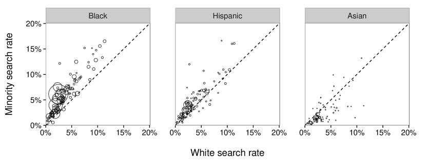
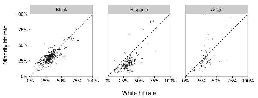
Adding resolution to these aggregate results, Fig. 3 compares search and hit rates for minorities and whites in each department. In the vast majority of cases, the top panel shows that blacks and Hispanics are searched at higher rates than whites. Asians, however, are consistently searched at lower rates than whites—indicating an absence of discrimination against Asians—in line with the aggregate results discussed above. The department-level outcome analysis is shown in the bottom panel of Fig. 3. In most departments, when Hispanics are searched, they are found to have contraband less often than searched whites, indicative of discrimination. However, hit rates for blacks and Asians are comparable to, or even higher than, hit rates for whites in a substantial fraction of cases, suggesting a lack of discrimination against these groups in many departments.

Both the benchmark and outcome tests suggest discrimination against blacks and Hispanics in the majority of police departments, but also yield conflicting results in a significant number of cases. For example, both tests are indicative of discrimination against blacks in 57 of the top 100 departments; but in 42 departments, they offer ambiguous evidence, with one test pointing toward discrimination against black drivers while the other indicates discrimination against white drivers. In one department both the outcome and benchmark tests point to discrimination against white drivers.

Results from the threshold test

We next use our threshold test to infer race- and department-specific search thresholds. Given the observed data, we estimate the posterior distribution of the search thresholds via Hamiltonian Monte Carlo (HMC) sampling (Neal, 1994; Duane et al., 1987), a form of Markov chain Monte Carlo sampling (Metropolis et al., 1953). We specifically use the No-U-Turn sampler (NUTS) (Hoffman and Gelman, 2014) as implemented in Stan (Carpenter et al., 2016), an open-source modeling language for full Bayesian statistical inference. To assess convergence of the algorithm, we sampled five Markov chains in parallel and computed the potential scale reduction factor $\hat{R}$ (Gelman and Rubin, 1992). We found that 2,500 warmup iterations and 2,500 sampling iterations per chain were sufficient for convergence, as indicated by $\hat{R}$ values less than $1.05$ for all parameters, as well as by visual inspection of the trace plots.

Figure 4: Inferred search thresholds in the 100 largest North Carolina police departments. Each point compares the search thresholds applied to minority and white drivers in a department, where points are scaled to the number of times the minority race was stopped by the department. In nearly every department, black and Hispanic drivers face lower search thresholds than whites, suggestive of discrimination.

Figure 5: Race-specific search thresholds and signal distributions, averaged over all departments and where we weight by the total number of stops conducted by the department. We find that black and Hispanic drivers face substantially lower search thresholds than white and Asian drivers.

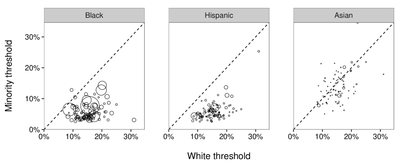
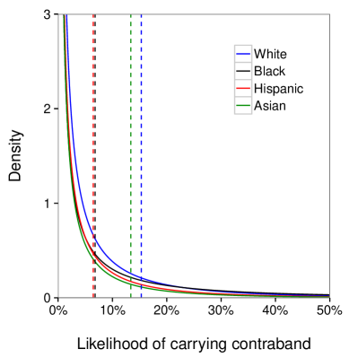
Figure 4 shows the posterior mean search thresholds for each race and department. Each point in the plot corresponds to a department, and compares the search threshold for whites (on the $x$-axis) to that for minorities (on the $y$-axis). In nearly all the departments we consider, the inferred search thresholds for black and Hispanic drivers are lower than for whites, suggestive of discrimination against these groups. For Asians, in contrast, the inferred search thresholds are generally in line with those of whites, indicating an absence of discrimination against Asians in search decisions.

Figure 5 displays the average, state-wide inferred signal distributions and thresholds for whites, blacks, Hispanics, and Asians. These averages are computed by weighting the department-level results by the number of stops in the department. Specifically, the overall race-specific threshold $t_{r}$ is given by $\left(\sum_{d}t_{rd}\cdot n_{d}\right)/\sum_{d}n_{d}$, where $n_{d}$ is the number of stops in department $d$. Similarly, the aggregate signal distributions show the department-weighted distribution of probabilities of possessing contraband. As is visually apparent, and also summarized in Table 2, the inferred thresholds for searching whites (15%) and Asians (13%) are significantly higher than the inferred thresholds for searching blacks (7%) and Hispanics (6%). These thresholds are estimated to about $\pm 2\%$, as indicated by the 95% credible intervals listed in Table 2.

Driver race Search threshold 95% credible interval White 15% (14%, 16%) Black 7% (3%, 10%) Hispanic 6% (5%, 8%) Asian 13% (11%, 16%)

Table 2: Inferred search thresholds for stops conducted by the 100 largest police departments in North Carolina. For each race group, we report the average threshold across departments, weighting by the number of stops conducted by the department. We find black and Hispanic drivers face lower search thresholds than white and Asian drivers.

Figure 6: Inferred search thresholds and signal distributions for black and white drivers stopped by the Raleigh Police Department, illustrating the problem of infra-marginality. The heavier tail of the black signal distribution means that searches of blacks have a higher hit rate despite black drivers facing a lower search threshold than whites. Hence, the outcome test concludes white drivers are being discriminated against, whereas the threshold test finds discrimination against black drivers.

The effects of infra-marginality

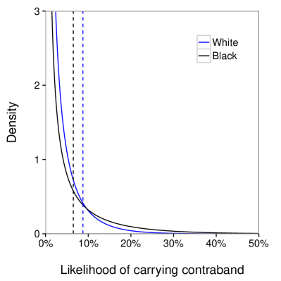
Why is it that the threshold test shows consistent discrimination against blacks and Hispanics when benchmark and outcome analysis suggest a more ambiguous story? To understand this dissonance, we examine the specific case of the Raleigh Police Department, the second largest department in North Carolina by number of stops recorded in our dataset. Black drivers in Raleigh are searched at a higher rate than whites (4% vs. 2%), but when searched, blacks are also found to have contraband at a higher rate (16% vs. 13%). The benchmark and outcome tests thus yield conflicting assessments of whether black drivers face discrimination. Figure 6 shows the inferred signal distributions and thresholds for white and black drivers in Raleigh, and sheds light on these seemingly contradictory results. The signal distribution for black drivers has a heavier right tail—for example, there is four times more mass above 20% than in the white distribution. This suggests that officers can more easily determine which black drivers are carrying contraband, which causes their searches of blacks to be more successful than their searches of whites. In spite of the higher hit rate for black drivers, we find that blacks still face a lower search threshold (6%) than whites (9%), suggesting discrimination against blacks.

Despite the theoretical advantages of the threshold test, it is difficult to know for sure whether the threshold test or the outcome test better reflects decision making in Raleigh. We note, though, three reasons that suggest the threshold test is the more accurate one. First, looking at Hispanic drivers in Raleigh, both the benchmark and outcome tests indicate they face discrimination. Hispanic drivers are searched more often than whites (3% vs. 2%), and are found to have contraband less often (11% vs. 13%). The threshold test likewise finds evidence of discrimination against Hispanics. The outcome test applied to black drivers is thus the odd one out: the benchmark, outcome, and threshold tests all point to discrimination against Hispanic drivers, and the benchmark and threshold tests suggest discrimination against black drivers. Second, the outcome test indicates not only an absence of discrimination, but that white drivers face substantial bias; while possible, that conclusion is at odds with past empirical research on traffic stops (Epp et al., 2014). Finally, the data suggest a compelling explanation for the heavier tail in the inferred signal distribution for black drivers: stopped blacks may be more likely than whites to carry contraband in plain view, as indicated by the fact that stops of blacks are three times more likely to end in searches based on “observation of suspected contraband”. The Raleigh Police Department thus appears to be a real-world example in which infra-marginality leads the outcome test to produce spurious results.

Model checks

We now evaluate in more detail how well our analytic approach explains the observed patterns in the North Carolina traffic stop data, and examine the robustness of our conclusions to violations of the model assumptions.

Posterior predictive checks.

We begin by investigating the extent to which the fitted model yields race- and department-specific search and hit rates that are in line with the observed data. Specifically, for each department and race group, we compare the observed search and hit rates to their expected values under the assumed data-generating process with parameters drawn from the inferred posterior distribution. Such posterior predictive checks (Gelman et al., 2014, 1996) are a common approach for identifying and measuring systematic differences between a fitted Bayesian model and the data.

We compute the posterior predictive search and hit rates as follows. During model inference, our Markov chain Monte Carlo sampling procedure yields 2,500 draws from the joint posterior distribution of the parameters. For each parameter draw—consisting of $\{\phi_{r}^{*}\}$, $\{\lambda_{r}^{*}\}$, $\{\phi_{d}^{*}\}$, $\{\lambda_{d}^{*}\}$ and $\{t_{rd}^{*}\}$—we analytically compute the search and hit rates $s_{rd}^{*}$ and $h_{rd}^{*}$ for each race-department pair implied by the data-generating process with those parameters. Finally, we average these search and hit rates over all 2,500 posterior draws.

(a)

(b)

Figure 7: Comparison of model-implied search and hit rates to the actual, observed values. Each point is a race-department pair, with points sized by number of stops. The plots show that the fitted model captures key features of the observed data. The root mean squared prediction error (weighted by stop count) is 0.1% for search rate and is 2.9% for hit rate.

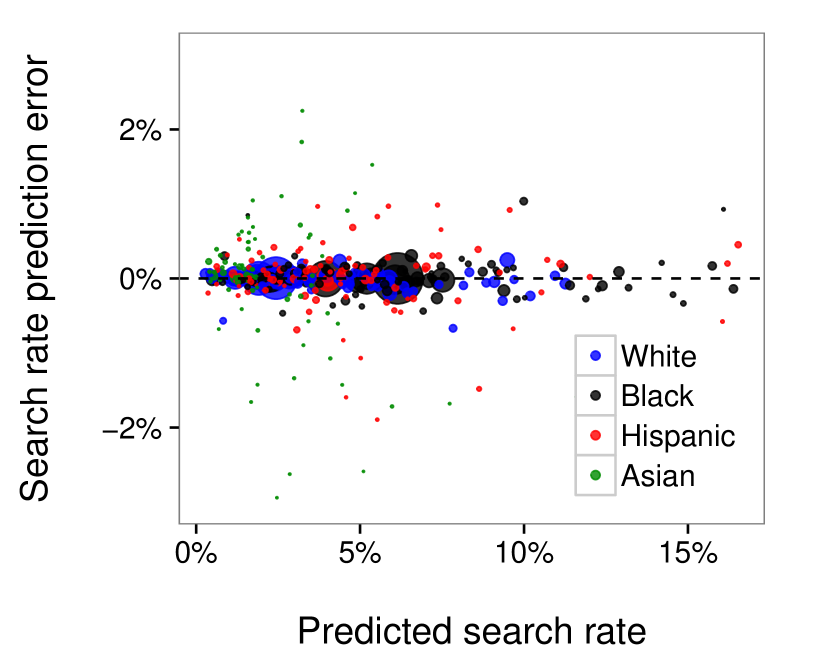
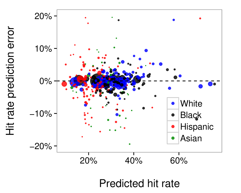
Figure 7 compares the model-predicted search and hit rates to the actual, observed values. Each point in the plot corresponds to a single race-department group, where groups are sized by number of stops. The fitted model recovers the observed search rates almost perfectly across races and departments. The fitted hit rates also agree with the data quite well, with the largest groups exhibiting almost no error. These posterior predictive checks thus indicate that the fitted model captures key features of the observed data.

Heterogeneous search thresholds.

Figure 8: Inferred race-specific search thresholds for synthetic data generated under a model in which thresholds randomly vary from one stop to the next. The dashed horizontal lines show the average of the thresholds used to generate the data. Model inferences are largely robust to stop-level heterogeneity in search thresholds.

Our behavioral model assumes that there is a single search threshold for each race-department pair. In reality, officers within a department might apply different thresholds, and even the same officer might vary the threshold he or she applies from one stop to the next. Moreover, officers only observe noisy approximations of a driver’s likelihood of carrying contraband; such errors can be equivalently recast as variation in the search threshold applied to the true probability.

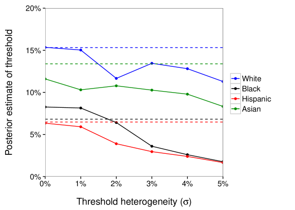
To investigate the robustness of our approach and results to such heterogeneity, we examine the stability of our inferences on synthetic datasets derived from a generative process with varying thresholds. Specifically, we start with the model fit to the actual data and then proceed in four steps. First, for each observed stop, we draw a signal $p$ from the inferred signal distribution for the department $d$ in which the stop occurred and the race $r$ of the motorist. Second, we set the stop-specific threshold to $T\sim\text{N}(t_{rd},\sigma)$, where $t_{rd}$ is the inferred threshold, and $\sigma$ is a parameter we set to control the degree of heterogeneity in the thresholds. Third, we assume a search occurs if and only if $p\geq T$, and if a search is conducted, we assume contraband is found with probability $p$. Finally, we use our modeling framework to infer new search thresholds $t_{rd}^{\prime}$ for the synthetic dataset. Figure 8 plots the result of this exercise for $\sigma$ varying between 0 and 0.05. It shows that the inferences are relatively stable throughout this range, and in particular, that there is a persistent gap between whites and Asians compared to blacks and Hispanics. We note that a five percentage point change in the thresholds is quite large. For example, decreasing the search threshold of blacks by five points in each department would more than triple the overall state-wide search rate of blacks.

Omitted variable bias.

As we discussed in Section 2, our approach is robust to unobserved heterogeneity that affects the signal, since we effectively marginalize over any omitted variables when estimating the signal distribution. However, we must still worry about systematic variation in the thresholds that is correlated with race. For example, if officers apply a lower search threshold at night, and black drivers are disproportionately likely to be stopped at night, then blacks would, on average, experience a lower search threshold than whites even in the absence of discrimination. Fortunately, as a matter of policy, only a limited number of factors may legitimately affect the search thresholds, and many—but not all—of these are recorded in the data. As a point of comparison, there are a multitude of hard-to-quantify factors (such as socio-economic indicators, or behavioral cues) that may, and likely do, affect the signal, but these should not affect the threshold.

Figure 9: Inferred search thresholds by race when the model is fit separately on various subsets of the data. Points indicate posterior means and are sized according to the number of stops in the subset. We consistently observe that blacks and Hispanics face lower search thresholds than whites.

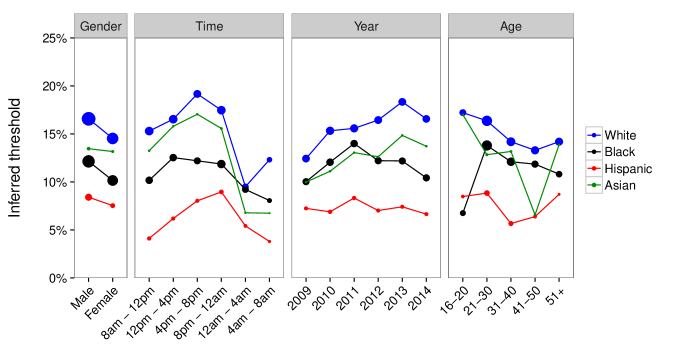
Our model already explicitly accounts for search thresholds that vary by department. We now examine the robustness of our results when adjusting for possible variation across year, time-of-day, age, and gender of the driver. Specifically, we disaggregate our primary dataset by year (and, separately, by time-of-day, by age, and by gender), and then independently run the threshold test on each component. Figure 9 shows the results of this analysis, and illustrates two points. First, we find that the inferred thresholds do indeed vary across the different subsets of the data. Second, in every case, the thresholds for searching blacks and Hispanics are lower than the threshold for searching whites, corroborating our main results.

In addition to the factors considered above, officers may legally apply a lower search threshold in situations involving officer safety. In particular, “protective frisks” require only reasonable suspicion, a lower standard of evidence than the probable cause requirement that applies to most searches. Further, probationers in North Carolina are subject to the reasonable suspicion standard regardless of safety issues. Similarly, searches “incident to arrest” are often carried out as a matter of policy before transporting arrestees, and so such searches may have a near-zero threshold. If stopped black and Hispanic drivers are more likely than whites to fall into these categories (e.g., if blacks and Hispanics are more likely to be on probation), then the lower average search thresholds we find for minorities may not be the product of discrimination. To test for this possibility, we now say a “search” has occurred only if: (1) the basis for the search is recorded as “probable cause”; and (2) “other official info” was not indicated as a precipitating factor. The latter restriction is intended to exclude searches triggered by a driver’s probation status. Repeating our analysis with searches redefined in this way, we find the basic pattern still holds: blacks and Hispanics are searched at lower thresholds (8% and 21%, respectively) than whites and Asians (40% and 38%, respectively). The inferred thresholds are higher than in our primary analysis—as expected, since we restricted to searches subject to a higher standard—but the gap remains.

A final potential confound is that search thresholds may vary by the severity of the contraband an officer believes could be present. For example, if officers have a lower threshold for searching drivers when they suspect possession of cocaine rather than marijuana, and black and Hispanic drivers are disproportionately likely to be suspected of carrying cocaine, then the threshold test could mistakenly infer discrimination where there is none. Unfortunately, the suspected offense motivating a search is not recorded in our data, and so we cannot directly test for such an effect, constituting one important limit of our statistical analysis.

Placebo tests.

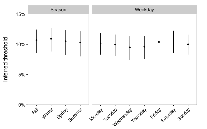
Finally, we conduct two placebo tests, where we rerun our threshold test with race replaced by day-of-week, and separately, with race replaced by season. The hope is that the threshold test accurately captures a lack of “discrimination” based on these factors. Figure 10 shows that the model indeed finds that the threshold for searching individuals is relatively stable by day-of-week, with largely overlapping credible intervals. We similarly find only small differences in the inferred seasonal thresholds. We note that some variation is expected, as officers might legitimately apply slightly different search standards throughout the week or year.

Figure 10: Results of placebo tests, in which we examine how search thresholds vary by season and day-of-week. Points show the posterior means, and the bars indicate 95% credible intervals. The threshold test accurately suggests a lack of “discrimination” in these cases.

Conclusion

Theoretical limitations with the two most widely used tests for discrimination—the benchmark and outcome tests—have hindered investigations of bias. Addressing this challenge, we have developed a new statistical approach to detecting discrimination that builds on the strengths of the benchmark and outcome tests and that mitigates the shortcomings of both. On a dataset of 4.5 million motor vehicle stops in North Carolina, our threshold test suggests that black and Hispanic motorists face discrimination in search decisions. Further, by specifically examining the Raleigh Police Department, we find that the problem of infra-marginality appears to be more than a theoretical possibility, and may have caused the outcome test to mistakenly conclude that officers discriminated against white drivers.

Our empirical results appear robust to reasonable violations of the model assumptions, including noise in estimates of the likelihood a driver is carrying contraband. We have also attempted to rule out some of the more obvious legitimate reasons for which thresholds might vary, including search policies that differ across department, year, or time of day. However, as with all tests of discrimination, there is a limit to what one can conclude from such statistical analysis alone. For example, if search policies differ not only across but also within department, then the threshold test could mistakenly indicate discrimination where there is none. Such within-department variation might result from explicit policy choices, or as a by-product of deployment patterns; in particular, the marginal cost of conducting a search may be lower in heavily policed neighborhoods, potentially justifying a lower search threshold in those areas. Additionally, if officers suspect more serious criminal activity when searching black and Hispanic drivers compared to whites, then the lower inferred search thresholds for these groups may be the result of non-discriminatory factors. To a large extent, such limitations apply equally to past tests of discrimination, and as with those tests, caution is warranted when interpreting the results.

Aside from police practices, the threshold test could be applied to study discrimination in a variety of settings where benchmark and outcome analysis is the status quo, including lending, hiring, and publication decisions. Looking forward, we hope our methodological approach spurs further investigation into the theoretical properties of statistical tests of discrimination, as well as their practical application.

References

- Alpert et al. (2004) Geoffrey P Alpert, Michael R Smith, and Roger G Dunham. Toward a better benchmark: Assessing the utility of not-at-fault traffic crash data in racial profiling research. Justice Research and Policy, 6(1):43–69, 2004.
- Antonovics and Knight (2009) Kate Antonovics and Brian G Knight. A new look at racial profiling: Evidence from the Boston police department. The Review of Economics and Statistics, 91(1):163–177, 2009.
- Anwar and Fang (2006) Shamena Anwar and Hanming Fang. An alternative test of racial prejudice in motor vehicle searches: Theory and evidence. The American Economic Review, 2006.
- Arrow (1973) Kenneth Arrow. The theory of discrimination. In Discrimination in Labor Markets. Princeton University Press, 1973.
- Ayres (2002) Ian Ayres. Outcome tests of racial disparities in police practices. Justice Research and Policy, 4(1-2):131–142, 2002.
- Becker (1957) Gary S Becker. The economics of discrimination. University of Chicago Press, 1957.
- Becker (1993) Gary S Becker. Nobel lecture: The economic way of looking at behavior. Journal of Political Economy, pages 385–409, 1993.
- Carpenter et al. (2016) Bob Carpenter, Andrew Gelman, Matt Hoffman, Daniel Lee, Ben Goodrich, Michael Betancourt, Marcus A Brubaker, Jiqiang Guo, Peter Li, and Allen Riddell. Stan: A probabilistic programming language. Journal of Statistical Software, 2016.
- Carr et al. (1993) James H Carr, Isaac F Megbolugbe, et al. The Federal Reserve Bank of Boston study on mortgage lending revisited. Fannie Mae Office of Housing Policy Research, 1993.
- Duane et al. (1987) Simon Duane, Anthony D Kennedy, Brian J Pendleton, and Duncan Roweth. Hybrid Monte Carlo. Physics Letters B, 195(2):216–222, 1987.
- Engel and Calnon (2004) Robin S Engel and Jennifer M Calnon. Comparing benchmark methodologies for police-citizen contacts: Traffic stop data collection for the Pennsylvania State Police. Police Quarterly, 7(1):97–125, 2004.
- Engel and Tillyer (2008) Robin S Engel and Rob Tillyer. Searching for equilibrium: The tenuous nature of the outcome test. Justice Quarterly, 25(1):54–71, 2008.
- Epp et al. (2014) Charles R Epp, Steven Maynard-Moody, and Donald P Haider-Markel. Pulled over: How police stops define race and citizenship. University of Chicago Press, 2014.
- Galster (1993) George C Galster. The facts of lending discrimination cannot be argued away by examining default rates. Housing Policy Debate, 4(1):141–146, 1993.
- Gelman and Rubin (1992) Andrew Gelman and Donald B Rubin. Inference from iterative simulation using multiple sequences. Statistical Science, pages 457–472, 1992.
- Gelman et al. (1996) Andrew Gelman, Xiao-Li Meng, and Hal Stern. Posterior predictive assessment of model fitness via realized discrepancies. Statistica Sinica, 6(4):733–760, 1996.
- Gelman et al. (2007) Andrew Gelman, Jeffrey Fagan, and Alex Kiss. An analysis of the New York City Police Department’s “stop-and-frisk” policy in the context of claims of racial bias. Journal of the American Statistical Association, 102(479), 2007.
- Gelman et al. (2014) Andrew Gelman, John B Carlin, Hal S Stern, and Donald B Rubin. Bayesian data analysis. Taylor & Francis, 2nd edition, 2014.
- Goel et al. (2016) Sharad Goel, Justin M Rao, and Ravi Shroff. Precinct or prejudice? Understanding racial disparities in New York City’s stop-and-frisk policy. Annals of Applied Statistics, 2016.
- Goel et al. (2017) Sharad Goel, Maya Perelman, Ravi Shroff, and David Sklansky. Combatting police discrimination in the age of big data. New Criminal Law Review, 20, 2017.
- Grogger and Ridgeway (2006) Jeffrey Grogger and Greg Ridgeway. Testing for racial profiling in traffic stops from behind a veil of darkness. Journal of the American Statistical Association, 101(475), September 2006.
- Hetey et al. (2016) Rebecca Hetey, Benoît Monin, Amrita Maitreyi, and Jennifer Eberhardt. Data for change: A statistical analysis of police stops, searches, handcuffings, and arrests in oakland, calif., 2013-2014. Technical report, Stanford University, SPARQ: Social Psychological Answers to Real-World Questions, 2016.
- Hoffman and Gelman (2014) Matthew D Hoffman and Andrew Gelman. The No-U-Turn Sampler: Adaptively setting path lengths in Hamiltonian Monte Carlo. Journal of Machine Learning Research, 15(Apr):1593–1623, 2014.
- Jordan (2004) Michael I Jordan. Graphical models. Statistical Science, pages 140–155, 2004.
- Knowles et al. (2001) John Knowles, Nicola Persico, and Petra Todd. Racial bias in motor vehicle searches: Theory and evidence. Journal of Political Economy, 109(1), 2001.
- Lange et al. (2001) James E Lange, Kenneth O Blackman, and Mark B Johnson. Speed violation survey of the New Jersey Turnpike: Final report. Public Services Research Institute, 2001.
- Maclin (2008) Tracey Maclin. Good and bad news about consent searches in the Supreme Court. McGeorge L. Rev., 39:27, 2008.
- McConnell and Scheidegger (2001) Elizabeth H McConnell and Amie R Scheidegger. Race and speeding citations: Comparing speeding citations issued by air traffic officers with those issued by ground traffic officers. In Annual meeting of the Academy of Criminal Justice Sciences, Washington, DC, 2001.
- Metropolis et al. (1953) Nicholas Metropolis, Arianna W Rosenbluth, Marshall N Rosenbluth, Augusta H Teller, and Edward Teller. Equation of state calculations by fast computing machines. The Journal of Chemical Physics, 21(6):1087–1092, 1953.
- Neal (1994) Radford M Neal. An improved acceptance procedure for the hybrid Monte Carlo algorithm. Journal of Computational Physics, 111(1):194–203, 1994.
- Phelps (1972) Edmund S Phelps. The statistical theory of racism and sexism. The American Economic Review, 62(4):659–661, 1972.
- Pierson et al. (2017) Emma Pierson, Sam Corbett-Davies, and Sharad Goel. Fast threshold tests for detecting discrimination. Preprint available at https://arxiv.org/abs/1702.08536, 2017.
- Ridgeway (2006) Greg Ridgeway. Assessing the effect of race bias in post-traffic stop outcomes using propensity scores. Journal of Quantitative Criminology, 22(1):1–29, 2006.
- Ridgeway and MacDonald (2009) Greg Ridgeway and John M MacDonald. Doubly robust internal benchmarking and false discovery rates for detecting racial bias in police stops. Journal of the American Statistical Association, 104(486):661–668, 2009.
- Walker (2003) Samuel Walker. Internal benchmarking for traffic stop data: An early intervention system approach. Technical report, Police Executive Research Forum, 2003.