The length of the low-redshift standard ruler

Abstract

Assuming the existence of standard rulers, standard candles and standard clocks, requiring only the cosmological principle, a metric theory of gravity, a smooth expansion history, and using state-of-the-art observations, we determine the length of the “low-redshift standard ruler”. The data we use are a compilation of recent Baryon acoustic oscillation data (relying on the standard ruler), Type 1A supernovæ (as standard candles), ages of early type galaxies (as standard clocks) and local determinations of the Hubble constant (as a local anchor of the cosmic distance scale). In a standard $\Lambda$CDM cosmology the “low-redshift standard ruler” coincides with the sound horizon at radiation drag, which can also be determined –in a model dependent way– from CMB observations. However, in general, the two quantities need not coincide. We obtain constraints on the length of the low-redshift standard ruler: $r^{h}_{\rm s}=101.0\pm 2.3h^{-1}$ Mpc, when using only Type 1A supernovæ and Baryon acoustic oscillations, and $r_{\rm s}=150.0\pm 4.7$ Mpc when using clocks to set the Hubble normalisation, while $r_{\rm s}=141.0\pm 5.5$ Mpc when using the local Hubble constant determination (using both yields $r_{\rm s}=143.9\pm 3.1$ Mpc).

The low-redshift determination of the standard ruler has an error which is competitive with the model-dependent determination from cosmic microwave background measurements made with the Planck satellite, which assumes it is the sound horizon at the end of baryon drag.

1 Introduction

We build on the idea presented in Sutherland (2012) and Heavens, Jimenez & Verde (2014) that relatively low redshift measurements of the cosmic expansion history $H(z)$, can be used, in combination with measurements of the Baryon Acoustic Oscillation (BAO) feature, to determine the length of a standard ruler in a model-independent way. Supernovae type 1A are standard(izable) candles yielding a luminosity-distance – redshift relation. The BAO feature is probably the best-understood standard ruler in the Universe. However, it has the drawback that the comoving length of the ruler, the sound horizon at radiation drag $r_{\rm s}$, is usually calibrated at $z>1000$ relying on Cosmic Microwave Background (CMB) observations and theoretical assumptions. Without knowing the length of the ruler or the brightness of the candles or the Hubble parameter, these probes can only give relative measurements of the expansion history. The quantities $r_{\rm s}$ and $H_{0}$ provide absolute scales for distance measurements (anchors) at opposite ends of the observable Universe. But while the CMB $r_{\rm s}$ determination depends on several assumptions (standard gravity, standard radiation content, negligible isocurvature perturbations, standard scaling of matter and radiation components, negligible early dark energy etc.), local determinations of the expansion rate are cosmology-independent. Alternatively standard clocks (Jimenez & Loeb, 2002) can be used, representing objects whose age is determined by established physics, and whose formation time is sufficiently early that scatter amongst formation times is negligible in the present cosmological context. Standard clocks provide (absolute) measurements of $H(z)$.

Even relative measurements of the expansion history, from observations of Type 1A supernovæ, in combination with measurements of the BAO feature can yield a constraint on the low-redshift standard ruler, $r^{h}_{\rm s}$, which is the ruler length in units of $h^{-1}$Mpc. An absolute distance scale can be provided by adding a constraint on $h$ such as that provided by $H_{0}$ or clocks, in which case observations of the BAO feature can be used to determine the absolute length of the low-redshift standard ruler, $r_{\rm s}$, in units of Mpc. The importance of this scale is that it is a key theoretical prediction of cosmological models, depending on the sound speed and expansion rate of the Universe at early times, before matter and radiation decouple. However the low-redshift standard ruler is a direct measurement, which will survive even if the standard cosmological model and standard assumptions about early-time physics do not. Since the analysis of Heavens, Jimenez & Verde (2014), new BAO, $H_{0}$, and cosmic clock data have become available, with improved statistics, which we consider here.

2 Data and Methodology

The latest $H_{0}$ determination is provided by the SH0ES program, reaching a 2.4% precision, $H_{0}^{SH0ES}=73.24\pm 1.74$ km s^-1Mpc^-1 (Riess et al., 2016). A Gaussian likelihood is assumed.

The supernovæ  type 1A data are the compilation of Betoule et al. (2014), binned into 31 redshift intervals between $0$ and $1.3$, equally-spaced in $\log(1+z)$ to yield the distance modulus as function of redshift. The covariance matrix is supplied for the binned data. The binning, in conjunction with the central limit theorem, motivates the use of a gaussian likelihood. The data is given as measurements of the distance modulus

$$\mu(z)\equiv m-M=25+5\log_{10}D_{L}(z)$$ (1)

where $m$ is the apparent magnitude, $M$ a fiducial absolute magnitude $M\simeq-19.3$ and $D_{L}$ the luminosity distance.

Constraints on BAO are from the following galaxy surveys: Six Degree Field Galaxy Survey (6dF) (Beutler et al., 2011), the LOWZ and CMASS galaxy samples of the Baryon Oscillation Spectroscopic Survey (BOSS-LOWZ and BOSS-CMASS, respectively, Cuesta et al. (2016), we use the isotropic measurement), and the reanalysed measurements of WiggleZ (Blake et al., 2011) by Kazin et al. (2014). While we take into account the correlation among the WiggleZ measurements we neglect the correlation between WiggleZ and CMASS. This is motivated by the fact that the WiggleZ-CMASS overlap includes a small fraction of the BOSS-CMASS sample and the correlation is very small, always below 4% (Beutler et al., 2016; Cuesta et al., 2016). BAO data provide measurements of the dilation scale normalized by the standard ruler length, $D_{V}/r_{\rm s}$, where

$$D_{V}(z)\equiv\left[(1+z)^{2}D^{2}_{A}(z)\frac{cz}{H(z)}\right]^{1/3}.$$ (2)

If $r_{\rm s}$ is interpreted as the sound horizon at radiation drag, $r_{d}(z_{d})$, then

$$r_{d}(z_{d})=\int_{z_{d}}^{\infty}\frac{c_{s}(z)}{H(z)}dz,$$ (3)

where $c_{s}(z)$ is the sound speed.

For the standard clocks, we use galaxy ages determined from analysis of stellar populations of old elliptical galaxies. We assume that the formation time was at sufficiently high redshift that variations in formation time of stars within each galaxy and among galaxies are negligible. Differential ages, $\Delta t$, then provide estimates of the inverse Hubble parameter as $1/H(z)=dt/dz(1+z)$ and $dt/dz\simeq\Delta t/\Delta z$ for suitable redshift intervals $\Delta z$. We use the measurements of $H(z)$ obtained by Moresco et al. (2016), who extend the previously available compilation to include both a fine sampling at $0.38<z<0.48$ exploiting the unprecedented statistics provided by the BOSS Data Release 9, and the redshift range up to $z\sim 2$.

As in Heavens, Jimenez & Verde (2014), we parametrise the expansion history by an inverse Hubble parameter, ${\sf{h^{-1}}}(z)\equiv 100{\rm km}\,{\rm s}^{-1}{\rm Mpc}^{-1}/H(z)$, which is specified at $N=7$ values (nodes) equally-spaced between $z=0$ and $z=1.97$; we linearly-interpolate ${\sf{h^{-1}}}(z)$ in between. Since the maximum redshift probed by supernovæ  data is smaller than that probed by clocks, when clocks are not included $N=5$ and the maximum redshift value considered is $z=1.3$. This implicitly assumes a smooth expansion history.

Assuming the cosmological principle of homogeneity and isotropy (and thus a FRW metric), the curvature of the Universe ($k=\{1,0,-1\}$) and $H(z)$ completely specify the metric and the geometric observables considered here: luminosity distance $D_{L}$, and the dilation scale $D_{V}$ through the angular diameter distance $D_{A}$. The curvature radius of the Universe is $k\,R_{0}$ (for $k=\pm 1$) and infinity for $k=0$, where $R_{0}$ denotes the present value of the scale factor, and the curvature is $\kappa=c/(R_{0}H_{0})$. If we wish further to assume General Relativity (GR), the curvature density parameter is given by $\Omega_{k}=k[c/(R_{0}H_{0})]^{2}=k\kappa^{2}$ with $c$ the speed of light.

As it is customary for supernovæ, we allow an absolute magnitude offset $\Delta M$: we are assuming the existence of a standard candle, but not its luminosity. Similarly, for the BAO measurements, we assume there is a standard ruler, which is normally interpreted as the sound horizon at radiation drag, but for the purposes here, it is simply a ruler.

The parameters are therefore ($r_{\rm s}^{h}$, $\Omega_{k}$, $\Delta M$, ${\sf{h^{-1}}}(0)$, ${\sf{h^{-1}}}(z_{1})$,$\ldots,{\sf{h^{-1}}}(z_{N})$). Uniform priors are assumed for all parameters. The parameter space is explored via standard Monte Carlo Markov Chain (MCMC) methods.

In Sec. 3.1 we compare this parametrization with a prior on $H(z)$ in five knots, $r_{\rm s}$ and a spline interpolation. We also compare results for different sampling techniques: Metropolis Hastings (Hastings, 1970) and Affine Invariant sampler (Goodman & Weare, 2010).

Data	$r^{h}_{s}[h^{-1}\rm Mpc]$	$r_{\rm s}[\rm Mpc]$	$H_{0}$	$\Delta M$	$\Omega_{k}=k(c/H_{0}R_{0})^{2}$
SBH	$102.0\pm 2.5(^{+2.2}_{-2.8})$	$140.8\pm 4.9$	$72.8\pm 1.8$	$0.079\pm 0.083$	$-0.49\pm 0.64\,\left(-0.99^{+0.86}_{-0.26}\right)$
BH	$107.2\pm 7.2$	$147\pm 10$	$73.0\pm 1.8$	N/A	unconstrained
SB	$101.0\pm 2.3$	unconstrained	unconstrained	unconstrained	$0.07\pm 0.61$
CB	$103.9\pm 5.6$	$149.5\pm 4.3$	$69.6\pm 4.2$	N/A	unconstrained
CSB	$100.5\pm 1.9$	$150.0\pm 4.7$	$67.0\pm 2.5$	$-0.090\pm 0.079$	$0.36\pm 0.41$
CBH	$107.2\pm 3.4$	$148.0\pm 3.9$	$72.5\pm 1.7$	N/A	unconstrained
CSBH	$102.3\pm 1.8$	$143.9\pm 3.1$	$71.1\pm 1.5$	$0.028\pm 0.047$	$-0.03\pm 0.31\left(-0.08^{+0.32}_{-0.28}\right)$
SBH	$100.7\pm 1.8$	$138.5\pm 4.3$	$72.8\pm 1.8$	$0.083\pm 0.061$	flat
BH	$107.1\pm 7.2$	$147\pm 10$	$73.0\pm 1.8$	N/A	flat
SB	$101.2\pm 1.8$	unconstrained	unconstrained	unconstrained	flat
CB	$103.7\pm 5.5$	$149.8\pm 4.2$	$69.2\pm 4.0$	N/A	flat
CSB	$101.4\pm 1.7$	$148.3\pm 4.3$	$68.5\pm 2.1$	$-0.047\pm 0.064$	flat
CBH	$107.4\pm 3.4$	$148.0\pm 3.6$	$72.6\pm 1.7$	N/A	flat
CSBH	$102.3\pm 1.6$	$143.9\pm 3.1$	$71.1\pm 1.4$	$0.026\pm 0.043$	flat

Table 1: Posterior mean and standard deviation for the model parameters. The curvature radius of the Universe $R_{0}$ is constrained, independently of General Relativity, but we report it in terms of the GR-specific curvature density parameter $\Omega_{k}$. The curvature distribution in some cases is highly non-gaussian: therefore we also report in parenthesis the maximum of the posterior and the 68% highest posterior density interval. When SNe are not included $\Delta M$ is not a parameter (hence the “N/A” table entry).

Figure 1: At glance: comparison of central values and 1$\sigma$ errors on the $r_{\rm s}^{h}$ (left) and $r_{\rm s}$ (right) measurements for flat geometry (blue) and marginalizing over the curvature (black). Note the change of the scale in the x-axis in each figure.

3 Results

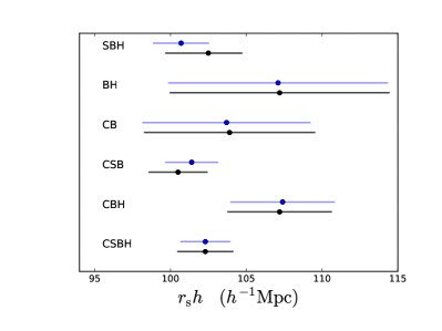
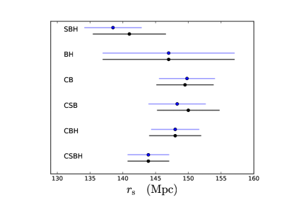
In table 1 we report the mean and 68% credible regions for the recovered quantities for various combinations of the data: CSBH indicating Clocks, supernovæ, BAOs, local $H_{0}$ respectively.

The posterior distribution of the curvature parameter is highly non-gaussian, except when both clocks and Supernovae data are considered or in the SB case; the curvature is poorly constrained otherwise, hence in these cases we also report the maximum of the posterior and the 68% highest posterior density interval.

Figure 2: Reconstructed expansion history $H(z)$ (95% confidence envelop) for two representative dataset combinations: SBH (left) CSBH (right). The last redshift nodes (one on the left, two on the right) are not shown as there $H(z)$ is poorly constrained. The jagged shape of the envelop is due to the linear interpolation being performed in $1/H$ while the quantity plotted is $H(z)$. Symbols represent the best fit values for the reconstruction.

The results of Tab. 1 indicate the following.

• There is only a mild dependence of the low-redshift standard ruler determination on curvature. Imposing flatness reduces slightly the error bars, and has no effect when all datasets are considered. Only in the case of SBH does imposing flatness induce a change of $\sim 1\sigma$ in the low-redshift standard ruler towards lower values.

• The recovered $H_{0}$ estimates cluster around two values: $h\equiv{\sf h}(z=0)\sim 0.73$ obtained when the local $H_{0}^{SH0ES}$ is used (as expected); and $h\sim 0.68$ when clocks are used, and $0.71$ when both are used.

• The $H_{0}$ value obtained by the CSB combination has an error bar of 3.7%, to be compared with a 2.4% error for $H_{0}^{SH0ES}$ and a 3.8% error for H0LiCOW (Bonvin et al., 2016). These two measurements are in agreement at the $2\sigma$ level with the CSB value.

• supernovæ  and cosmic clocks data are needed to constrain the curvature. The curvature distribution is highly non-gaussian, unless these data sets are considered.

• without $H_{0}^{SH0ES}$, $r_{\rm s}$ tends to be $\sim 149$Mpc, as expected, $H_{0}^{SH0ES}$ pulls the recovered $r_{\rm s}$ downwards.

• depending on how extensive the dataset considered is, the error on $r_{\rm s}^{h}$ varies between 7% (for BH) to 1.8% (CSBH), the error on $r_{\rm s}$ varies between 7% (for BH) to 2.1% (CSBH).

• while $r_{\rm s}^{h}$ is better determined than $r_{\rm s}$ the recovered value across different data sets is more consistent for $r_{\rm s}$.

• $r_{\rm s}^{h}$ is determined at the $2$% level with only BAO and Supernovae. In this case the curvature distribution is remarkably more symmetric than for the SBH case.

Figure 1 offers visual comparisons of the $r_{\rm s}^{h}$ and $r_{\rm s}$ measurements, for the flat case and marginalizing over curvature. The CSB combination yields a $r_{\rm s}$ value fully consistent with the Planck mission CMB inferred one, while the SBH determination yields lower values, which are still consistent in the case of the non-flat case but become a $\sim 2\sigma$ tension (with respect to the Planck value for the $\Lambda$CDM model) when flatness is imposed.

Figure 3: Effects of prior assumptions and MCMC sampling method. We show the comparison of the posterior distributions of $\Omega_{k}$ (left) and in the $\Omega_{k}$-$r_{\rm s}^{h}$ plane (right) obtained from the same data (SBH) with different methodologies: this work (blue), using an Affine Invariant sampler instead of Metropolis Hastings (red) with two choices for the redshift sampling, the one form this work (solid) and the one from BVR (dashed), and the approach of BVR (green), which uses Affine Invariant sampler, $r_{\rm s}$ and $H(z_{i})$ as variables and a spline interpolation of $H(z)$.

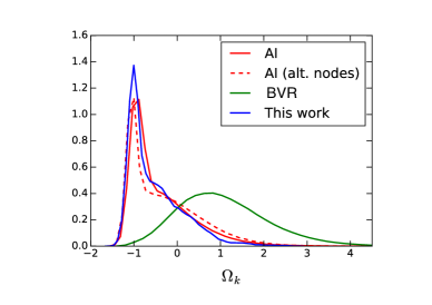
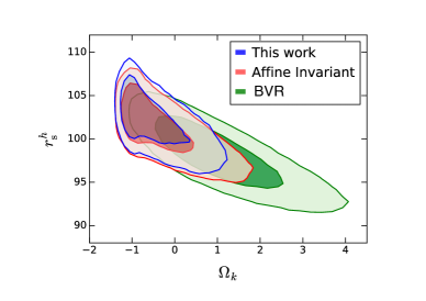
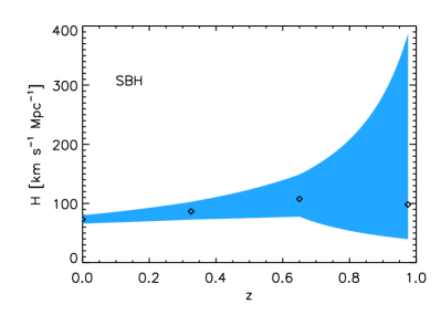
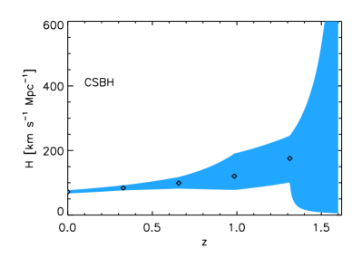
Fig.  2 shows the envelope enclosing 95% of the reconstructed $H(z)$ for two representative data set combinations. The odd shape of the envelope is due to the fact that the linear interpolation is being performed in $1/H$ while the quantity plotted is $H(z)$. Symbols represent the best fit $H(z)$ of each redshift. The highest redshift nodes are poorly constrained and therefore not shown. Also for the CSBH case, the joint distribution of the ${\sf{h^{-1}}}(z_{n})$ values for the last two redshift nodes. show a structure indicating a high degree of interdependence between the two quantities. This does not affect the determination of the standard ruler, as there is no correlation between $r_{\rm s}$ or $r_{\rm s}^{h}$ and ${\sf{h^{-1}}}(z_{n})$ for $n\geq 4$.

Figure 4: Effect of combining the low-redhisft standard ruler measurement (interpreted as the sound horizon at radiation drag) with CMB Planck observations. The transparent contours show the joint $r_{\rm s}$ vs $N_{\rm eff}$ 68% and 95% marginalised confidence regions obtained from the posterior sample provided by the Planck CMB mission. On the left, all temperature and polarisation data are used, on the right, high $\ell$ polarisation data are not included. The filled contours result from importance sampling this with our CSB measurement (top row), SBH (middle row) and CSBH (bottom row).

3.1 Robustness to prior assumptions

To assess the dependence on the prior assumptions, we compare our findings with the results and the approach of Bernal, Riess & Verde (2016)(BVR). In that work, a similar reconstruction of the late time expansion history is performed in the context of the study of the tension between the (direct) local $H_{0}$ determination and its CMB-inferred value within the $\Lambda$CDM model. However, they use a different parametrization and sampling method: $H(z)$ and $r_{\rm s}$ are the free parameters and $H(z)$ values are interpolated using natural cubic splines, instead of $r_{\rm s}^{h}$, ${\sf{h^{-1}}}(z)$ and linear interpolation as done here. They also use an Affine Invariant sampler (implemented in the public code emcee (Foreman-Mackey et al., 2013)) instead of Metropolis Hastings. BVR does not include cosmic clocks, so we concentrate on SBH data combination for this test. The number of nodes is the same ($N=5$), although their location is different. We isolate each of the methodological differences to study their effect in the final results.

As supernovæ  data impose very strong constraints on the shape of $H(z)$, the resulting expansion history does not depend on the interpolation method, even taking into account that the splines allow much more freedom than the linear interpolation. Also, the location of the knots does not have any significant effect in the final fit of the reconstruction. It does however have a mild effect on the curvature, which is the parameter most weakly constrained.

In Fig. 3 we show the posterior distribution of $\Omega_{k}$ (left) and the joint distribution in the $\Omega_{k}$-$r_{\rm s}^{h}$ plane (right) for the different cases compared in this section. The distributions are marginalised over all other parameters. We refer as ‘Affine Invariant’ to the case when the only change with respect to this work is the MCMC sampler. The figure also quantifies the effect of a different choice of redshift sampling (nodes). Unlike in our parametrization, using $r_{\rm s}$ and $H(z)$ as free parameters makes the distribution of $\Omega_{k}$ Gaussian, but centered around higher values and with larger error bars.

As $r_{\rm s}$ and $\Omega_{k}$ are anticorrelated (and $\Omega_{k}$ and $H_{0}$ are independent), differences in the posterior of $\Omega_{k}$ result in different determinations of the low-redshift standard ruler. The values of $r_{\rm s}$ and $r_{\rm s}^{h}$ obtained in this work (for the non-flat case) are $\sim 1\sigma$ higher than in BVR. Once flatness is imposed, the discrepancies between the two sampling algorithms and prior choices disappear.

It is important to point out that the dependence of the posterior on the prior choice and the MCMC sampling method only appears when the parameters are weakly constrained. This is the case when using only BAO, supernovæ and $H_{0}$ (SBH) and not imposing flatness. Both cosmic clocks and supernovæ data are needed to obtain a Gaussian posterior distribution for the curvature: in these cases (CSBH and CSB), the dependence on the prior assumptions and the sampler becomes unimportant. The dependence on prior is negligible also for the SBH dataset combination when flatness is imposed.

4 Discussion and conclusions

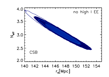
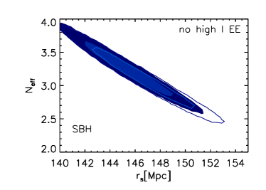
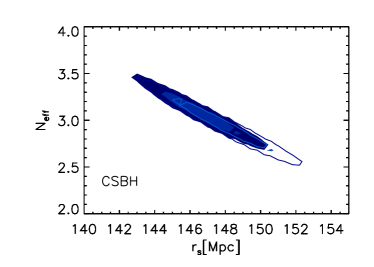
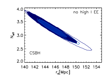
This model-independent determination of the low-redshift standard ruler can be interpreted as the sound horizon at the baryon drag and thus compared with (model-dependent) CMB determinations. This comparison can be used to limit the scope of new physics that may alter the early expansion rate and sound speed. This is investigated in detail for example in Verde et al. (2016). Here we only compare our constraints with those obtained by the Planck team with the Planck 2015 data release, using publicly available posterior samples (Planck Collaboration, Ade et al., 2015). The direct measurement of the ruler is in good agreement with the CMB-derived one for all models considered by the Planck team and especially the standard $\Lambda$CDM model. In all cases the CMB-inferred error bars, are, understandably, much smaller, with one notable exception: the model where the effective number of neutrino species is free (Heavens, Jimenez & Verde, 2014). The effect of combining our measurement with the CMB one is illustrated in Fig. 4. Transparent contours are the (joint) 68% and 95% confidence regions for CMB data alone including (excluding) high $\ell$ polarisation data on the left (right) panel. The filled contours result from importance sampling this with our SBH, CSB or CSBH, measurement, which reduce the errors significantly. When $H_{0}^{SH0ES}$ is included the error on $N_{\rm eff}$ is reduced by suppressing the posterior for low $N_{\rm eff}$ values. A similar trend was found by Riess et al. (2016) and by Bernal, Riess & Verde (2016).

Note that even without an estimate of $h$, the combination of BAO and Supernovæ data already constrain the low-redshift standard ruler scale $r_{s}^{h}$ at the 2% level, $r_{s}^{h}=101.0\pm 2.3$ Mpc/$h$.

Looking ahead, improvements on the low-redshift standard ruler measurement may arise from the next generation of BAO surveys. For example, if in the CSB (or CSBH) combination we substitute the current BAO measurements with forecasted constraints achievable with a survey with the specifications of DESI (Levi et al., 2013), errors without imposing flatness will reduce as follows. The error on $r_{\rm s}^{h}$ will go from $1.9$% to $1.3$% ($1.8$% to $1.1$%), the error on $r_{\rm s}$ from 3.2% to 2.8% (2.2% to 1.9%) the error on $H_{0}$ from 3.7% to 3.4% (2.1% to 2%) and the error on $\Omega_{k}$ from $\pm 0.41$ to $\pm 0.28$ ($\pm 0.31$ to $\pm 0.22$). Given the dramatic improvement in the precision of expansion history constraints provided by the next generation of BAO surveys, these forecasts indicate that we are entering a regime where the error on $r_{\rm s}$ is dominated by that on the normalisation of the expansion history $h$, and therefore directly or indirectly on $H_{0}$. Improvement on the local $H_{0}$ determination towards a goal of $\sim 1$% error budget may be provided by e.g., gravitational lensing time delays (Suyu et al., 2016) and by further improvements of the classic distance ladder approach (Riess et al., 2016).

5 acknowledgements

LV and JLB thank A. Riess for discussions. RJ and LV acknowledge support from Mineco grant AYA2014-58747-P and MDM-2014-0369 of ICCUB (Unidad de Excelencia Maria de Maeztu), and a visiting scientist grant from the Royal Society. JLB is supported by the Spanish MINECO under grant BES-2015-071307, co-funded by the ESF. JLB and AFH acknowledges hospitality of Radcliffe Institute for Advanced Study, Harvard University. AFH, RJ and LV acknowledge Imperial College for support under the CosmoCLASSIC collaboration.

Based on observations obtained with Planck (http://www.esa.int/Planck), an ESA science mission with instruments and contributions directly funded by ESA Member States, NASA, and Canada.

Funding for SDSS-III has been provided by the Alfred P. Sloan Foundation, the Participating Institutions, the National Science Foundation, and the U.S. Department of Energy Office of Science. The SDSS-III web site is http://www.sdss3.org/.

SDSS-III is managed by the Astrophysical Research Consortium for the Participating Institutions of the SDSS-III Collaboration including the University of Arizona, the Brazilian Participation Group, Brookhaven National Laboratory, Carnegie Mellon University, University of Florida, the French Participation Group, the German Participation Group, Harvard University, the Instituto de Astrofisica de Canarias, the Michigan State/Notre Dame/JINA Participation Group, Johns Hopkins University, Lawrence Berkeley National Laboratory, Max Planck Institute for Astrophysics, Max Planck Institute for Extraterrestrial Physics, New Mexico State University, New York University, Ohio State University, Pennsylvania State University, University of Portsmouth, Princeton University, the Spanish Participation Group, University of Tokyo, University of Utah, Vanderbilt University, University of Virginia, University of Washington, and Yale University.

References

- Bernal, Riess & Verde (2016) Bernal J. L., Riess A. G., Verde L., 2016, in preparation
- Betoule et al. (2014) Betoule M., et al., 2014, Astron. Astrophys., 568, A22
- Beutler et al. (2011) Beutler F. et al., 2011, Mon. Not. Roy. Astron. Soc., 416, 3017
- Beutler et al. (2016) Beutler F., Blake C., Koda J., Marín F. A., Seo H.-J., Cuesta A. J., Schneider D. P., 2016, Mon. Not. Roy. Astron. Soc., 455, 3230
- Blake et al. (2011) Blake C. et al., 2011, Mon. Not. Roy. Astron. Soc., 418, 1707
- Bonvin et al. (2016) Bonvin V., et al., 2016, ArXiv:1607.01790
- Cuesta et al. (2016) Cuesta A. J. et al., 2016, Mon. Not. Roy. Astron. Soc., 457, 1770
- Foreman-Mackey et al. (2013) Foreman-Mackey D., Hogg D. W., Lang D., Goodman J., 2013, Publications of the Astronomical Society of the Pacific, 125, 306
- Goodman & Weare (2010) Goodman J., Weare J., 2010, Comm. App. Math. Comp., 5, 65
- Hastings (1970) Hastings W. K., 1970, Biometrika, 57, 97
- Heavens, Jimenez & Verde (2014) Heavens A., Jimenez R., Verde L., 2014, Phys. Rev. Lett., 113, 241302
- Jimenez & Loeb (2002) Jimenez R., Loeb A., 2002, Astrophys. J., 573, 37
- Kazin et al. (2014) Kazin E. A. et al., 2014, Mon. Not. Roy. Astron. Soc., 441, 3524
- Levi et al. (2013) Levi M. et al., 2013, ArXiv:1308.0847
- Moresco et al. (2016) Moresco M. et al., 2016, JCAP, 5, 014
- Planck Collaboration, Ade et al. (2015) Planck Collaboration, Ade P. A. R., et al., 2015, ArXiv:1502.01589
- Riess et al. (2016) Riess A. G. et al., 2016, ArXiv:1604.01424
- Sutherland (2012) Sutherland W., 2012, Mon. Not. Roy. Astron. Soc., 426, 1280
- Suyu et al. (2016) Suyu S. H. et al., 2016, ArXiv:1607.00017
- Verde et al. (2016) Verde L., et al., 2016, in preparation