Algorithm xxx: SC-SR1: MATLAB Software for Limited-Memory SR1 Trust-Region Methods

Abstract.

We present a MATLAB implementation of the symmetric rank-one (SC-SR1) method that solves trust-region subproblems when a limited-memory symmetric rank-one (L-SR1) matrix is used in place of the true Hessian matrix, which can be used for large-scale optimization. The method takes advantage of two shape-changing norms [1, 2] to decompose the trust-region subproblem into two separate problems. Using one of the proposed norms, the resulting subproblems have closed-form solutions. Meanwhile, using the other proposed norm, one of the resulting subproblems has a closed-form solution while the other is easily solvable using techniques that exploit the structure of L-SR1 matrices. Numerical results suggest that the SC-SR1 method is able to solve trust-region subproblems to high accuracy even in the so-called “hard case”. When integrated into a trust-region algorithm, extensive numerical experiments suggest that the proposed algorithms perform well, when compared with widely used solvers, such as truncated CG.

1. Introduction

At each iteration of a trust-region method for minimizing a general nonconvex function $f(\mathbf{x})$, the so-called trust-region subproblem must be solved to obtain a step direction:

$${\displaystyle\mathop{\operator@font{minimize}}_{\mathbf{p}\in\mathbb{R}^{n}}}\;\;{\mathcal{Q}}\left(\mathbf{p}\right)\mathop{\,{\scriptstyle\stackrel{{\scriptstyle\triangle}}{{=}}}}\,\mathbf{g}^{T}\mathbf{p}+\frac{1}{2}\mathbf{p}^{T}\mathbf{B}\mathbf{p}\;\;\;\mathop{\operator@font{subject\ to}}\;\;\|\mathbf{p}\|\leq\delta,$$ (1)

where $\mathbf{g}\mathop{\,{\scriptstyle\stackrel{{\scriptstyle\triangle}}{{=}}}}\,\nabla f\left(\mathbf{x}_{k}\right)$, $\mathbf{B}$ is an approximation to $\nabla^{2}f\left(\mathbf{x}_{k}\right)$, $\delta$ is a positive constant, and $\|\cdot\|$ is a given norm. In this article, we describe a MATLAB implementation for solving the trust-region subproblem (1) when $\mathbf{B}$ is a limited-memory symmetric rank-one (L-SR1) matrix approximation of $\nabla^{2}f(\mathbf{x}_{k})$. In large-scale optimization, solving (1) represents the bulk of the computational effort in trust-region methods. The norm used in (1) not only defines the trust region shape but also determines the difficulty of solving each subproblem.

The most widely-used norm chosen to define the trust-region subproblem is the two-norm. One reason for this choice of norm is that the necessary and sufficient conditions for a global solution to the subproblem defined by the two-norm are well-known [3, 4, 5]; many methods exploit these conditions to compute high-accuracy solutions to the trust-region subproblem (see e.g., [6, 7, 8, 9, 10, 4]). The infinity-norm is sometimes used to define the subproblem; however, when $\mathbf{B}$ is indefinite, as can be the case when $\mathbf{B}$ is a L-SR1 matrix, the subproblem is NP-hard [11, 12]. For more discussion on norms other than the infinity-norm we refer the reader to [13].

In this article, we consider the trust-region subproblems defined by shape-changing norms originally proposed in [1]. Generally speaking, shape-changing norms are norms that depend on $\mathbf{B}$; thus, in the quasi-Newton setting where the quasi-Newton matrix $\mathbf{B}$ is updated each iteration, the shape of the trust region changes each iteration. One of the earliest references to shape-changing norms is found in [14] where a norm is implicitly defined by the product of a permutation matrix and a unit lower triangular matrix that arise from a symmetric indefinite factorization of $\mathbf{B}$. Perhaps the most widely-used shape-changing norm is the so-called “elliptic norm” given by $\|\mathbf{x}\|_{A}\mathop{\,{\scriptstyle\stackrel{{\scriptstyle\triangle}}{{=}}}}\,\mathbf{x}^{T}\mathbf{Ax}$, where $\mathbf{A}$ is a positive-definite matrix (see, e.g., [13]). A well-known use of this norm is found in the Steihaug method [15], and, more generally, truncated preconditioned conjugate-gradients (CG) [13]; these methods reformulate a two-norm trust-region subproblem using an elliptic norm to maintain the property that the iterates from preconditioned CG are increasing in norm. Other examples of shape-changing norms include those defined by vectors in the span of $\mathbf{B}$ (see, e.g., [13]).

The shape-changing norms proposed in [1, 2] have the advantage of breaking the trust-region subproblem into two separate subproblems. Using one of the proposed shape-changing norms, the solution of the subproblem then has a closed-form solution. In the other proposed norm, one of the subproblems has a closed-form solution while the other is easily solvable. The publicly-available LMTR codes [16] solve trust-region subproblems (1) defined by these shape-changing norms and the limited-memory Broyden-Fletcher-Goldfarb-Shanno (L-BFGS) updates of $\mathbf{B}$. To our knowledge, there are no other implementations for solving trust-region subproblems defined by these shape-changing norms.

1.1. Overview of the proposed method

In this paper, we develop a MATLAB implementation for solving trust-region (TR) subproblems defined by the two shape-changing norms described in [1] when L-SR1 approximations to the Hessian are used instead of L-BFGS approximations. For limited-memory algorithms a re-scaling strategy (i.e., effectively re-initializing the Hessian approximation at each iteration) is often important for the practical performance of the method. Yet, because the structure of L-SR1 matrices can be exploited to reduce the memory usage even further when a constant initialization is used (i.e., no re-scaling) we provide an option to chose between such strategies. Moreover, our implementation enables the testing and addition of new solvers by swapping out the respective TR subproblem algorithm. In this way, we conduct numerical experiments on large-scale CUTEst problems [17], comparing the shape-changing methods to truncated CG and an $\ell_{2}$-norm based algorithm. The proposed method, called the shape-changing SR1 method (SC-SR1), enables high-accuracy subproblem solutions by exploiting the structure of L-SR1 matrices.

This paper is organized as follows: In Section 2, we review L-SR1 matrices, including the compact representation for these matrices and a method to efficiently compute their eigenvalues and a partial eigenbasis. In Section 3, we demonstrate how the shape-changing norms decouple the original trust-region subproblem into two problems and describe the proposed solver for each subproblem. Finally, for each shape-changing norm, we show how to construct a global solution to (1) from the solutions of the two decoupled subproblems. Optimality conditions are presented for each of these decoupled subproblems in Section 4. In Section 5, we demonstrate the accuracy of the proposed solvers, and compare them on a collection of large-scale optimization problems. Concluding remarks can be found in Section 6.

1.2. Notation

In this article, the identity matrix of dimension $d$ is denoted by $\mathbf{I}_{d}=\left[\mathbf{e}_{1}|\cdots|\mathbf{e}_{d}\right]$, and depending on the context the subscript $d$ may be suppressed. Finally, we assume that all L-SR1 updates are computed so that the L-SR1 matrix is well defined.

2. L-SR1 matrices

Suppose $f:\mathbb{R}^{n}\rightarrow\mathbb{R}$ is a smooth objective function and $\{{\mathbf{x}}_{i}\}$, $i=0,\ldots k$, is a sequence of iterates, then the symmetric rank-one (SR1) matrix is defined using pairs $(\mathbf{s}_{i},\mathbf{y}_{i})$ where

$$\mathbf{s}_{i}\mathop{\,{\scriptstyle\stackrel{{\scriptstyle\triangle}}{{=}}}}\,\mathbf{x}_{i+1}-\mathbf{x}_{i}\quad\text{and}\quad\mathbf{y}_{i}\mathop{\,{\scriptstyle\stackrel{{\scriptstyle\triangle}}{{=}}}}\,\nabla f(\mathbf{x}_{i+1})-\nabla f(\mathbf{x}_{i}),$$

and $\nabla f$ denotes the gradient of $f$. Specifically, given an initial matrix $\mathbf{B}_{0}$, $\mathbf{B}_{k+1}$ is defined recursively as

$$\mathbf{B}_{k+1}\mathop{\,{\scriptstyle\stackrel{{\scriptstyle\triangle}}{{=}}}}\,\mathbf{B}_{k}+\frac{(\mathbf{y}_{k}-\mathbf{B}_{k}\mathbf{s}_{k})(\mathbf{y}_{k}-\mathbf{B}_{k}\mathbf{s}_{k})^{T}}{(\mathbf{y}_{k}-\mathbf{B}_{k}\mathbf{s}_{k})^{T}\mathbf{s}_{k}},$$ (2)

provided $(\mathbf{y}_{k}-\mathbf{B}_{k}\mathbf{s}_{k})^{T}\mathbf{s}_{k}\neq 0$. In practice, $\mathbf{B}_{0}=\mathbf{B}^{(k)}_{0}$ is often taken to be a scalar multiple of the identity matrix that re-scales $\mathbf{B}_{k}$ each iteration; for the duration of this article we assume that $\mathbf{B}_{0}=\gamma_{k}\mathbf{I}$, $\gamma_{k}\in\mathbb{R}$. Limited-memory symmetric rank-one matrices (L-SR1) store and make use of only the $m$ most-recently computed pairs $\{(\mathbf{s}_{i},\mathbf{y}_{i})\}$, where $m\ll n$ (for example, Byrd et al. [18] suggest $m\in[3,7]$). For simplicity of notation, we assume that the current iteration number $k$ is less than the number of allowed stored limited-memory pairs $m$.

The SR1 update is a member of the Broyden class of updates (see, e.g., [19]). Unlike widely-used updates such as the Broyden-Fletcher-Goldfarb-Shanno (BFGS) and the Davidon-Fletcher-Powell (DFP) updates, this update can yield indefinite matrices; that is, SR1 matrices can incorporate negative curvature information. In fact, the SR1 update has convergence properties superior to other widely-used positive-definite quasi-Newton matrices such as BFGS; in particular, [20] give conditions under which the SR1 update formula generates a sequence of matrices that converge to the true Hessian. (For more background on the SR1 update formula, see, e.g., [21, 22, 23, 19, 24, 25].)

2.1. Compact representation

The compact representation of SR1 matrices can be used to compute the eigenvalues and a partial eigenbasis of these matrices. In this section, we review the compact formulation of SR1 matrices.

To begin, we define the following matrices:

$$\mathbf{S}_{k} \mathop{\,{\scriptstyle\stackrel{{\scriptstyle\triangle}}{{=}}}}\, [\ \mathbf{s}_{0}\ \ \mathbf{s}_{1}\ \ \mathbf{s}_{2}\ \ \cdots\ \ \mathbf{s}_{k-1}\ ]\ \in\ \mathbb{R}^{n\times k},$$

$$\mathbf{Y}_{k} \mathop{\,{\scriptstyle\stackrel{{\scriptstyle\triangle}}{{=}}}}\, [\ \mathbf{y}_{0}\ \ \mathbf{y}_{1}\ \ \mathbf{y}_{2}\ \ \cdots\ \ \mathbf{y}_{k-1}\ ]\ \in\ \mathbb{R}^{n\times k}.$$

The matrix $\mathbf{S}_{k}^{T}\mathbf{Y}_{k}\in\mathbb{R}^{k\times k}$ can be written as the sum of the following three matrices:

$$\mathbf{S}_{k}^{T}\mathbf{Y}_{k}=\mathbf{L}_{k}+\mathbf{D}_{k}+\mathbf{R}_{k},$$

where $\mathbf{L}_{k}$ is strictly lower triangular, $\mathbf{D}_{k}$ is diagonal, and $\mathbf{R}_{k}$ is strictly upper triangular. Then, $\mathbf{B}_{k}$ can be written as

$$\mathbf{B}_{k}\ =\ \gamma_{k}\mathbf{I}+\mathbf{\Psi}_{k}\mathbf{M}_{k}\mathbf{\Psi}_{k}^{T},$$ (3)

where $\mathbf{\Psi}_{k}\in\mathbb{R}^{n\times k}$ and $\mathbf{M}_{k}\in\mathbb{R}^{k\times k}$. In particular, $\mathbf{\Psi}_{k}$ and $\mathbf{M}_{k}$ are given by

$$\mathbf{\Psi}_{k}\ =\ \mathbf{Y}_{k}-\gamma_{k}\mathbf{S}_{k}\quad\text{and}\quad\mathbf{M}_{k}\ =\ (\mathbf{D}_{k}+\mathbf{L}_{k}+\mathbf{L}_{k}^{T}-\gamma_{k}\mathbf{S}_{k}^{T}\mathbf{S}_{k})^{-1}.$$ (4)

The right side of equation (3) is the compact representation of $\mathbf{B}_{k}$; this representation is due to Byrd et al. [18, Theorem 5.1]. For the duration of this paper, we assume that updates are made when both the next SR1 matrix $\mathbf{B}_{k}$ is well-defined and $\mathbf{M}_{k}$ exists [18, Theorem 5.1]. For notational simplicity, we assume $\mathbf{\Psi}_{k}$ has full column rank; when $\mathbf{\Psi}_{k}$ does not have full column rank, we refer to [2] for the modifications needed for computing the eigenvalues, which we also review in Section 2.2. Notice that the computation of $\mathbf{M}_{k}$ is computationally admissible since it is a very small symmetric square matrix.

2.2. Limited-Memory Updating

For large optimization problems, limited-memory approaches store only a small number of vectors to define the L-SR1 representations. Depending on the initialization strategy, specifically whether $\gamma_{k}$ varies between iterations or is constant ($\gamma_{k}=\bar{\gamma}$) the matrices in (4) can be effectively stored and updated. We will describe these techniques in subsequent sections. By setting the parameter $m\ll n$ limited-memory techniques enable inexpensive computations, and replace or insert one column at each iteration in $\mathbf{Y}_{k}$ and $\mathbf{S}_{k}$. Let an underline below a matrix represent the matrix with its first column removed. That is, $\underline{\mathbf{S}}_{k}$ represents $\mathbf{S}_{k}$ without its first column. With this notation, a column update of a matrix, say $\mathbf{S}_{k}$, by a vector $\mathbf{s}_{k}$ is defined as follows.

$$\text{colUpdate}\left(\mathbf{S}_{k},\mathbf{s}_{k}\right)\mathop{\,{\scriptstyle\stackrel{{\scriptstyle\triangle}}{{=}}}}\,\begin{cases}[\>\mathbf{S}_{k}\>\mathbf{s}_{k}\>]&\text{ if }k<m\\ [\>\underline{\mathbf{S}}_{k}\>\mathbf{s}_{k}\>]&\text{ if }k\geq m.\\ \end{cases}$$

This column update can be implemented efficiently, without copying large amounts of memory, by appropriately updating a vector that stores index information (“mIdx”). A function to do so is described in Procedure 1:

0:  [$\mathbf{S}_{k}$,mIdx]=colUpdate($\mathbf{S}_{k}$, $\mathbf{s}_{k}$, mIdx, $m$, $k$);

1:  if $k=0$ then

2:     $\text{mIdx}\leftarrow\text{zeros}(m,1)$;

3:  end if

4:  if $k<m$ then

5:     $\text{mIdx}(k+1)\leftarrow k+1$;

6:     $\mathbf{S}_{k}(:,\text{mIdx}(k+1))\leftarrow\mathbf{s}_{k}$;

7:  else if $m\leq k$ then

8:     $k_{m}\leftarrow\text{mIdx}(1)$;

9:     $\text{mIdx}(1:(m-1))\leftarrow\text{mIdx}(2:m)$;

10:     $\text{mIdx}(m)\leftarrow k_{m}$;

11:     $\mathbf{S}_{k}(:,\text{mIdx}(m))\leftarrow\mathbf{s}_{k}$;

12:  end if

13:  return  $\mathbf{S}_{k}$, mIdx;

PROCEDURE 1 Limited-memory column updating of $\mathbf{S}_{k}$ by the vector $\mathbf{s}_{k}$

Note that this procedure does not copy (or overwrite) large blocks of memory as would commands such as $\{\mathbf{S}_{k}(:,1:(m-1))\leftarrow\mathbf{S}_{k}(:,2:m);\mathbf{S}_{k}(:,m)\leftarrow\mathbf{s}_{k}\}$, but instead accesses the relevant locations using a stored vector of indices. Certain matrix products can also be efficiently updated. As such, the product $\mathbf{S}_{k}^{T}\mathbf{Y}_{k}$ does not have to be re-computed from scratch. In order to describe the matrix product updating mechanism, let an overline above a matrix represent the matrix with its first row removed. That is, $\overline{\mathbf{S}^{T}_{k}\mathbf{Y}}_{k}$ represents $\mathbf{S}^{T}_{k}\mathbf{Y}_{k}$ without its first row. With this notation, a product update of, say $\mathbf{S}_{k}^{T}\mathbf{Y}_{k}$, by matrices $\mathbf{S}_{k}$, $\mathbf{Y}_{k}$ and vectors $\mathbf{s}_{k}$, $\mathbf{y}_{k}$ is defined as:

$$\text{prodUpdate}\left(\mathbf{S}_{k}^{T}\mathbf{Y}_{k},\mathbf{S}_{k},\mathbf{Y}_{k},\mathbf{s}_{k},\mathbf{y}_{k}\right)\mathop{\,{\scriptstyle\stackrel{{\scriptstyle\triangle}}{{=}}}}\,\begin{cases}\left[\begin{array}[]{ c c }\mathbf{S}_{k}^{T}\mathbf{Y}_{k}&\mathbf{S}_{k}^{T}\mathbf{y}_{k}\\ \mathbf{s}_{k}^{T}\mathbf{Y}_{k}&\mathbf{s}_{k}^{T}\mathbf{y}_{k}\end{array}\right]&\text{ if }k<m\vspace{0.1cm}\\ \left[\begin{array}[]{ c c }\left(\underline{\overline{\mathbf{S}^{T}_{k}\mathbf{Y}_{k}}}\right)&\underline{\mathbf{S}}_{k}^{T}\mathbf{y}_{k}\\ \mathbf{s}_{k}^{T}\underline{\mathbf{Y}}_{k}&\mathbf{s}_{k}^{T}\mathbf{y}_{k}\end{array}\right]&\text{ if }k\geq m.\\ \end{cases}$$

This product update can be implemented without recomputing potentially large multiplications, by storing previous products and information about the column order in $\mathbf{S}_{k}$ and $\mathbf{Y}_{k}$. In particular, updating the matrix product is based on storing $\mathbf{S}_{k}^{T}\mathbf{Y}_{k}$, $\mathbf{S}_{k},\mathbf{Y}_{k}$ and the vector “mIdx”. Although a different order is possible, we apply the product update after column updates of $\mathbf{S}_{k},\mathbf{Y}_{k}$ have been done previously. In such a situation the vector, which stores the appropriate index information (“mIdx”) is defined at such a point.

0:  [$\mathbf{S}_{k}^{T}\mathbf{Y}_{k}$]=prodUpdate($\mathbf{S}_{k}^{T}\mathbf{Y}_{k}$, $\mathbf{S}_{k}$, $\mathbf{Y}_{k}$, $\mathbf{s}_{k}$, $\mathbf{y}_{k}$, mIdx, $m$, $k$);

1:  if $k<m$ then

2:     $\mathbf{S}_{k}^{T}\mathbf{Y}_{k}(1:(k+1),k+1)\leftarrow\mathbf{S}_{k}(:,\text{mIdx}(1:(k+1)))^{T}\mathbf{y}_{k}$;

3:     $\mathbf{S}_{k}^{T}\mathbf{Y}_{k}(k+1,1:k)\leftarrow\mathbf{s}_{k}^{T}\mathbf{Y}_{k}(:,\text{mIdx}(1:k))$;

4:  else if $m\leq k$ then

5:     $\mathbf{S}_{k}^{T}\mathbf{Y}_{k}(1:(m-1),1:(m-1))\leftarrow\mathbf{S}_{k}^{T}\mathbf{Y}_{k}(2:m,2:m)$;

6:     $\mathbf{S}_{k}^{T}\mathbf{Y}_{k}(1:m,m)\leftarrow\mathbf{S}_{k}(:,\text{mIdx}(1:m)^{T}\mathbf{y}_{k}$;

7:     $\mathbf{S}_{k}^{T}\mathbf{Y}_{k}(m,1:(m-1))\leftarrow\mathbf{s}_{k}^{T}\mathbf{Y}_{k}(:,\text{mIdx}(1:(m-1)))$;

8:  end if

9:  return  $\mathbf{S}_{k}^{T}\mathbf{Y}_{k}$;

PROCEDURE 2 Limited-memory product update $\mathbf{S}_{k}^{T}\mathbf{Y}_{k}$ ($\mathbf{s}_{k}$, $\mathbf{y}_{k}$ are column updates to $\mathbf{S}_{k}$, $\mathbf{Y}_{k}$)

Note that such a product update is computationally much more efficient, than recomputing the product from scratch. Specifically, when $m\leq k$, the direct product $\mathbf{S}_{k}^{T}\mathbf{Y}_{k}$ is done at $\mathcal{O}(m^{2}n)$ multiplications. However, Procedure 2 does this update with $\mathcal{O}(2mn)$ multiplications in lines 6 and 7, by reusing previous values from line 5. Moreover, when the product is symmetric, e.g. Procedure 2 is invoked by $\texttt{prodUpdate}(\mathbf{S}_{k}^{T}\mathbf{S}_{k},\mathbf{S}_{k},\mathbf{S}_{k},\mathbf{s}_{k},\mathbf{s}_{k},\text{mIdx},m,k)$, then $\mathbf{S}_{k}(:,\text{mIdx}(1:m)^{T}\mathbf{s}_{k}$ can be stored in line 6 and reused in line 7 (thus only one matrix-vector product is needed, instead of two). Since limited-memory updating of the L-SR1 matrices varies for the chosen initialization strategy, we describe the cases of non-constant initializations $\gamma_{k}$ and constant $\gamma_{k}=\bar{\gamma}$ next.

2.2.1. Limited-memory updating of (4) using non-constant $\gamma_{k}$

When $\gamma_{k}$ varies for every iteration, $\boldsymbol{\Psi}_{k}$ is best implicitly represented by storing $\mathbf{S}_{k}$ and $\mathbf{Y}_{k}$, instead of explicitly forming it (forming $\boldsymbol{\Psi}_{k}$ explicitly incurs additional $\mathcal{O}(mn)$ memory locations in $\boldsymbol{\Psi}_{k}=\mathbf{Y}_{k}-\gamma_{k}\mathbf{S}_{k}$). By storing the previous $m$ pairs $\{\mathbf{s}_{i},\mathbf{y}_{i}\}_{i=k-m}^{k-1}$ in the limited-memory matrices $\mathbf{S}_{k}=[\>\mathbf{s}_{k-m}\>\cdots\>\mathbf{s}_{k-1}\>]\in\mathbb{R}^{n\times m}$ and $\mathbf{Y}_{k}=[\>\mathbf{y}_{k-m}\>\cdots\>\mathbf{y}_{k-1}\>]\in\mathbb{R}^{n\times m}$ the matrix-vector product $\boldsymbol{\Psi}_{k}^{T}\mathbf{g}$ (for a vector $\mathbf{g}$) is done as

$$\boldsymbol{\Psi}_{k}^{T}\mathbf{g}=\mathbf{Y}_{k}^{T}\mathbf{g}-\gamma_{k}(\mathbf{S}_{k}^{T}\mathbf{g}).$$

2.2.2. Limited-memory updating of (4) using constant $\gamma_{k}=\bar{\gamma}$

When $\gamma_{k}=\bar{\gamma}$ is constant, then $\mathbf{Y}_{k}$ and $\mathbf{S}_{k}$ do not have to be stored separately. Instead the limited-memory method stores $m$ previous vectors $\{\boldsymbol{\psi}_{i}=\mathbf{y}_{i}-\bar{\gamma}\mathbf{s}_{i}\}_{i=k-m}^{k-1}$, concatenated in the matrix

$$\boldsymbol{\Psi}_{k}=\left[\ \boldsymbol{\psi}_{k-m}\ \ \cdots\ \ \boldsymbol{\psi}_{k-1}\ \right]\in\mathbb{R}^{n\times m}$$

Matrix vector products are directly computed as $\boldsymbol{\Psi}_{k}^{T}\mathbf{g}_{k}$. Subsequently, $\mathbf{M}_{k}$ from (4) can be updated efficiently by noting that

$$\mathbf{M}_{k}^{-1}\mathbf{e}_{k}=\left(\mathbf{D}_{k}+\mathbf{L}_{k}+\mathbf{L}_{k}^{T}-\bar{\gamma}\mathbf{S}_{k}^{T}\mathbf{S}_{k}\right)\mathbf{e}_{k}=\boldsymbol{\Psi}_{k}^{T}\mathbf{s}_{k}.$$

Because of these simplifications an L-SR1 algorithm with constant initialization strategy can be implemented with about half the memory footprint (storing only $\boldsymbol{\Psi}_{k}$ as opposed to $\mathbf{Y}_{k},\mathbf{S}_{k}$ (and previous small products)). However, often the ability to rescale the computations via a non-constant $\gamma_{k}$ parameter can be advantageous in solving large-scale optimization problems. We provide an option to choose between constant or non-constant initialization strategies in our implementations.

2.3. Eigenvalues

In this subsection, we demonstrate how the eigenvalues and a partial eigenbasis can be computed for SR1 matrices. In general, this derivation can be done for any limited-memory quasi-Newton matrix that admits a compact representation; in particular, it can be done for any member of the Broyden convex class [26, 27, 28]. This discussion is based on [2].

Consider the problem of computing the eigenvalues of $\mathbf{B}_{k}$, which is assumed to be an L-SR1 matrix, obtained from performing $m$ rank-one updates to $\mathbf{B}_{0}=\mathbf{\gamma I}$. For notational simplicity, we drop subscripts and consider the compact representation of $\mathbf{B}$:

$$\mathbf{B}=\gamma\mathbf{I}+\mathbf{\Psi}\mathbf{M}\mathbf{\Psi}^{T}.$$ (5)

The “thin” QR factorization of $\mathbf{\Psi}$ can be written as $\mathbf{\Psi}=\mathbf{Q}\mathbf{R}$ where $\mathbf{Q}\in\mathbb{R}^{n\times m}$ and $\mathbf{R}\in\mathbb{R}^{m\times m}$ is invertible because, as it was assumed above, $\mathbf{\Psi}$ has full column rank. Then,

$$\mathbf{B}=\gamma\mathbf{I}+\mathbf{Q}\mathbf{R}\mathbf{M}\mathbf{R}^{T}\mathbf{Q}^{T}.$$ (6)

The matrix $\mathbf{RMR}^{T}\in\mathbb{R}^{m\times m}$ is of a relatively small size, and thus, it is computationally inexpensive to compute its spectral decomposition. We define the spectral decomposition of $\mathbf{R}\mathbf{M}\mathbf{R}^{T}$ as $\mathbf{U}\hat{\Lambda}\mathbf{U}^{T},$ where $\mathbf{U}\in\mathbb{R}^{m\times m}$ is an orthogonal matrix whose columns are made up of eigenvectors of $\mathbf{R}\mathbf{M}\mathbf{R}^{T}$ and $\hat{\Lambda}=\mathop{\operator@font diag}\nolimits(\hat{\lambda}_{1},\allowbreak\dots,\allowbreak\hat{\lambda}_{m})$ is a diagonal matrix whose entries are the associated eigenvalues.

Thus,

$$\mathbf{B}=\gamma\mathbf{I}+\mathbf{Q}\mathbf{U}\hat{\Lambda}\mathbf{U}^{T}\mathbf{Q}^{T}.$$ (7)

Since both $\mathbf{Q}$ and $\mathbf{U}$ have orthonormal columns, $\mathbf{P}_{\parallel}\mathop{\,{\scriptstyle\stackrel{{\scriptstyle\triangle}}{{=}}}}\,\mathbf{Q}\mathbf{U}\in\mathbb{R}^{n\times m}$ also has orthonormal columns. Let $\mathbf{P}_{\perp}$ denote the matrix whose columns form an orthonormal basis for $\left({\mathbf{P}}_{\parallel}\right)^{\perp}$. Thus, the spectral decomposition of $\mathbf{B}$ is defined as $\mathbf{B}=\mathbf{P}\Lambda_{\gamma}\mathbf{P}^{T},$ where

$$\mathbf{P}\mathop{\,{\scriptstyle\stackrel{{\scriptstyle\triangle}}{{=}}}}\,\begin{bmatrix}\mathbf{P_{\parallel}}\,\,\ \mathbf{P_{\perp}}\end{bmatrix}\quad\text{and}\quad\Lambda_{\gamma}\mathop{\,{\scriptstyle\stackrel{{\scriptstyle\triangle}}{{=}}}}\,\begin{bmatrix}\Lambda&0\\ 0&\gamma\mathbf{I}_{n-m}\end{bmatrix},$$ (8)

with $\Lambda_{\gamma}=\mathop{\operator@font diag}\nolimits(\lambda_{1},\ldots,\lambda_{n})$ and $\Lambda=\mathop{\operator@font diag}\nolimits(\lambda_{1},\ldots,\lambda_{m})=\hat{\Lambda}+\gamma\mathbf{I}\in\mathbb{R}^{m\times m}$.

We emphasize three important properties of the eigendecomposition. First, all eigenvalues of $\mathbf{B}$ are explicitly obtained and represented by $\Lambda_{\gamma}$. Second, only the first $m$ eigenvectors of $\mathbf{B}$ can be explicitly computed, if needed; they are represented by $\mathbf{P}_{\parallel}$. In particular, since $\mathbf{\Psi}=\mathbf{Q}\mathbf{R}$, then

$$\mathbf{P}_{\parallel}=\mathbf{Q}\mathbf{U}=\mathbf{\Psi}\mathbf{R}^{-1}\mathbf{U}.$$ (9)

If $\mathbf{P}_{\parallel}$ needs to only be available to compute matrix-vector products then one can avoid explicitly forming $\mathbf{P}_{\parallel}$ by storing $\mathbf{\Psi}$, $\mathbf{R}$, and $\mathbf{U}$. Third, the eigenvalues given by the parameter $\gamma$ can be interpreted as an estimate of the curvature of $f$ in the space spanned by the columns of $\mathbf{P}_{\perp}$.

While there is no reason to assume the function $f$ has negative curvature throughout the entire subspace $\mathbf{P}_{\perp}$, in this paper, we consider the case $\gamma\leq 0$ for the sake of completeness.

For the duration of this article, we assume the first $m$ eigenvalues in $\Lambda_{\gamma}$ are ordered in increasing values, i.e., $\Lambda=\mathop{\operator@font diag}\nolimits(\lambda_{1},\ldots,\lambda_{m})$ where $\lambda_{1}\leq\lambda_{2}\leq\ldots\leq\lambda_{m}$ and that $r$ is the multiplicity of $\lambda_{1}$, i.e., $\lambda_{1}=\lambda_{2}=\cdots=\lambda_{r}<\lambda_{r+1}$. For details on updating this partial spectral decomposition when a new quasi-Newton pair is computed, see [26].

2.4. Implementation

In the above presentation, the QR factorization was used for ease of readability to find a partial spectral decomposition of $\mathbf{B}$. However, there are other approaches that may be better suited for different applications. An alternative approach to computing the eigenvalues of $\mathbf{B}$ is presented in [29] that replaces the QR factorization of $\mathbf{\Psi}$ with the SVD and an eigendecomposition of a $m\times m$ matrix and $t\times t$ matrix, respectively, where $t\leq m$. (For more details, see [29].) However, experiments in [30] indicate that the QR version of this computation outperforms the SVD approach. When $\mathbf{\Psi}^{T}\mathbf{\Psi}$ is positive definite (i.e., $\mathbf{\Psi}$ is full rank), the Cholesky factorization of $\mathbf{\Psi}^{T}\mathbf{\Psi}=\mathbf{R}^{T}\mathbf{R}$ provides the same $\mathbf{R}$ needed to form $\mathbf{P}_{\parallel}$ in (9) [2]. Since $\boldsymbol{\Psi}$ is not explicitly formed when a non-constant initialization $\gamma=\gamma_{k}$ is used (in this case $\boldsymbol{\Psi}$ is defined by storing $\mathbf{Y},\mathbf{S}$) the product matrix $\boldsymbol{\Psi}^{T}\boldsymbol{\Psi}$ is represented by

$$\boldsymbol{\Psi}^{T}\boldsymbol{\Psi}=\mathbf{Y}^{T}\mathbf{Y}-2\gamma\mathbf{Y}^{T}\mathbf{S}+\gamma^{2}\mathbf{S}^{T}\mathbf{S}$$ (10)

(in (10) the matrices $\mathbf{Y}^{T}\mathbf{Y},\mathbf{Y}^{T}\mathbf{S}$ and $\mathbf{S}^{T}\mathbf{S}$ are stored and updated). In contrast, with a constant initialization $\gamma_{k}=\bar{\gamma}$ the product $\boldsymbol{\Psi}^{T}\boldsymbol{\Psi}$ can be directly updated.

For the algorithm proposed in this paper, it is necessary to be able to compute the eigenvalues of $\mathbf{B}$ and to be able to compute products with $\mathbf{P}_{\parallel}$. However, in our application, it could be the case that $\mathbf{\Psi}$ is not full rank; in this case, it is preferable to use the ${\small\text{LDL}^{T}}$ decomposition [31] of $\mathbf{\Psi}^{T}\mathbf{\Psi}$ as proposed in [2]. Specifically,

$$\mathbf{\Pi}^{T}\mathbf{\Psi}^{T}\mathbf{\Psi\Pi}=\mathbf{LDL}^{T},$$

where $\mathbf{\Pi}$ is a permutation matrix. If $\mathbf{\Psi}$ is rank-deficient, i.e., $\text{rank}(\mathbf{\Psi})=r<m$, then at least one diagonal entry of $\mathbf{D}$ is zero. (In computer arithmetic, it will be relatively small.) In the proposed algorithm, we use the following criteria to determine whether entries in $\mathbf{D}$ are sufficiently large: The $i$th entry of $\mathbf{D}$, i.e., $d_{i}$, is sufficiently large provided that

$${\color[rgb]{0,0,0}d_{i}>10^{-8}\times[\mathbf{\Pi}^{T}\mathbf{\Psi}^{T}\mathbf{\Psi\Pi}]_{ii}.}$$ (11)

Now, let $J$ to be the set of indices that satisfy (11), i.e., $r=|J|$. Furthermore, define $\mathbf{D}_{\dagger}$ to be the matrix $\mathbf{D}$ having removed any rows and columns indexed by an element not in $J$ and $\mathbf{L}_{\dagger}$ to be the matrix $\mathbf{L}$ having removed columns indexed by an element not in $J$. Then,

$$\mathbf{\Psi}^{T}\mathbf{\Psi}\approx\mathbf{\Pi L}_{\dagger}\mathbf{D}_{\dagger}\mathbf{L}^{T}_{\dagger}\mathbf{\Pi}^{T}=\mathbf{\Pi R}_{\dagger}^{T}\mathbf{R}_{\dagger}\mathbf{\Pi}^{T},$$

where $\mathbf{R}_{\dagger}\mathop{\,{\scriptstyle\stackrel{{\scriptstyle\triangle}}{{=}}}}\,\sqrt{\mathbf{D}_{\dagger}}\mathbf{L}_{\dagger}^{T}\in\mathbb{R}^{r\times m}$. Furthermore,

$$\mathbf{B}\approx\gamma\mathbf{I}+\mathbf{Q}_{\dagger}\mathbf{R}_{\dagger}\mathbf{\Pi}^{T}\mathbf{M\Pi}\mathbf{R}_{\dagger}^{T}\mathbf{Q}_{\dagger}^{T}\quad\text{with}\quad\mathbf{Q}_{\dagger}\mathop{\,{\scriptstyle\stackrel{{\scriptstyle\triangle}}{{=}}}}\,\left(\mathbf{\Psi\Pi}\right)_{\dagger}\mathbf{R}^{-1}_{\ddagger}\in\mathbb{R}^{n\times r},$$ (12)

where $\left(\mathbf{\Psi\Pi}\right)_{\dagger}$ is the matrix $\mathbf{\Psi\Pi}$ having deleted any columns indexed by an element not in $J$, and $\mathbf{R}_{\ddagger}\in\mathbb{R}^{r\times r}$ is the matrix $\mathbf{R}_{\dagger}$ having removed columns indexed by elements not in $J$. Notice that the matrix $\mathbf{R}_{\dagger}\mathbf{\Pi}^{T}\mathbf{M}\mathbf{\Pi}\mathbf{R}_{\dagger}^{T}\in\mathbb{R}^{r\times r}$ is full rank.

Thus, the eigenvalue decomposition $\mathbf{U}\hat{\Lambda}\mathbf{U}^{T}$ is now computed not for $\mathbf{RMR}^{T}$ as in Section 2.3, but for $\mathbf{R_{\dagger}\Pi}^{T}\mathbf{M\Pi R_{\dagger}}^{T}$. Furthermore, $\mathbf{P}_{\parallel}$ in (9) is computed as

$$\mathbf{P}_{\parallel}=\mathbf{Q_{\dagger}U}=\left(\mathbf{\Psi\Pi}\right)_{\dagger}\mathbf{R}_{\ddagger}^{-1}\mathbf{U}$$ (13)

when a constant initialization is used (since $\boldsymbol{\Psi}$ is explicitly formed), and as

$$\mathbf{P}_{\parallel}=\mathbf{Q_{\dagger}U}=\left(\mathbf{Y\Pi}\right)_{\dagger}\mathbf{R}_{\ddagger}^{-1}\mathbf{U}-\gamma\left(\mathbf{S\Pi}\right)_{\dagger}\mathbf{R}_{\ddagger}^{-1}\mathbf{U}$$ (14)

when a non-constant initialization is used.

Algorithm 1 details the computation of the elements needed to form $\mathbf{P}_{\parallel}$, using the ${\small\text{LDL}^{T}}$ decomposition. It produces $\mathbf{\Lambda}$, $\mathbf{R}_{\ddagger}$, $\mathbf{U}$, and $\mathbf{\Pi}$. There are several pre-processing and post-processing steps in this algorithm. Namely, lines 7 and 9 are used to remove any spurious complex round-off error, line 10 is to order the eigenvalues and associated eigenvectors, and line 12 sets any small eigenvalue (in absolute value) to zero. An alternative to forming and storing $\mathbf{R}_{\ddagger}$ is to maintain $\mathbf{R}_{\dagger}$ and the index set $J$. Moreover, since it is typically more efficient to update the product $\boldsymbol{\Psi}^{T}\boldsymbol{\Psi}$ instead of forming it from scratch, the argument “$\Psi\lor\Psi^{T}\Psi$” is used to enable passing either of the two inputs, depending on the context.

0:  [$\mathbf{R}_{\ddagger}$, $\mathbf{\Lambda}$, $\mathbf{U}$, $\mathbf{\Pi}$, $J$]=ComputeSpectral($\Psi\lor\Psi^{T}\Psi$, $\mathbf{M}^{-1}$, $\gamma$, $\tau$);

1:  Compute the ${\small\text{LDL}^{T}}$ decomposition of $\boldsymbol{\Psi}^{T}\boldsymbol{\Psi}$ and store the factors $\mathbf{L}$ and $\mathbf{D}$ matrices, and store $\mathbf{\Pi}$ (as a vector with the permutation information);

2:  Find the indices of elements of $\mathbf{D}$ that are sufficiently large using (11) and store as $J$;

3:  Form $\mathbf{D}_{\dagger}$ by storing the rows and columns of $\mathbf{D}$ corresponding to indices of $J$;

4:  Form $\mathbf{L}_{\dagger}$ by storing the columns of $\mathbf{L}$ corresponding the indices of $J$;

5:  $\mathbf{R}_{\dagger}\leftarrow\sqrt{\mathbf{D}_{\dagger}}\mathbf{L}_{\dagger}^{T}$;

6:  $\mathbf{T}\leftarrow\mathbf{R}_{\dagger}\mathbf{\Pi}^{T}\mathbf{M\Pi R}^{T}_{\dagger}$;

7:  Compute the spectral decomposition $\mathbf{U}\mathbf{\hat{\Lambda}}\mathbf{U}^{T}$of $(\mathbf{T}+\mathbf{T}^{T})/2$;

8:  Form $\mathbf{R}_{\ddagger}$ by storing the columns of $\mathbf{R}_{\dagger}$ corresponding to columns of $J$;

9:  $\mathbf{\hat{\Lambda}}\leftarrow\text{real}(\mathbf{\hat{\Lambda}})$

10:  Order the entries in $\mathbf{\hat{\Lambda}}$ from low to high and rearrange the columns of $\mathbf{U}$ accordingly to maintain the spectral decomposition of $(\mathbf{T}+\mathbf{T}^{T})/2$;

11:  $\mathbf{\Lambda}\leftarrow\mathbf{\hat{\Lambda}}+\gamma\mathbf{I}$;

12:  if $|\mathbf{\Lambda}_{ii}|<\tau$ for any $i$  then

13:     $\mathbf{\Lambda}_{ii}\leftarrow 0$;

14:  end if

15:  return  $\mathbf{R}_{\ddagger}$, $\mathbf{\Lambda}$, $\mathbf{U}$, $\mathbf{\Pi}$;

ALGORITHM 3 Computing $\mathbf{R}_{\ddagger}$, $\mathbf{\Lambda}$, $\mathbf{U}$, and $\mathbf{\Pi}$ using the ${\small\text{LDL}^{T}}$ decomposition

The output of Algorithm 1 includes the factors of $\mathbf{P}_{\parallel}$ (see (13)), i.e., $\mathbf{R}_{\ddagger}$, $\mathbf{U}$, and $\mathbf{\Pi}$, as well as $J$. For the method proposed in Section 3, products with $\mathbf{P}_{\parallel}$ are computed as a sequence of explicit matrix-vector products with the factors of $\mathbf{P}_{\parallel}$. In practice, the permutation matrix $\mathbf{\Pi}$ is not stored explicitly; instead, the permutation is applied implicitly using a vector that maintains the order of the columns after the permutation matrix is applied. Thus, products with $\mathbf{P}_{\parallel}$ are computed using only matrix-vector products together with a rearranging of columns.

3. Proposed method

The proposed method is able to solve the L-SR1 trust-region subproblem to high accuracy, even when $\mathbf{B}$ is indefinite. The method makes use of the eigenvalues of $\mathbf{B}$ and the factors of $\mathbf{P}_{\parallel}$. To describe the method, we first transform the trust-region subproblem (1) so that the quadratic objective function becomes separable. Then, we describe the shape-changing norms proposed in [1, 2] that decouples the separable problem into two minimization problems, one of which has a closed-form solution while the other can be solved very efficiently. Finally, we show how these solutions can be used to construct a solution to the original trust-region subproblem.

3.1. Transforming the Trust-Region Subproblem

Let $\mathbf{B}=\mathbf{P}\Lambda_{\gamma}\mathbf{P}^{T}$ be the eigendecomposition of $\mathbf{B}$ described in Section 2.2. Letting $\mathbf{v}=\mathbf{P}^{T}\mathbf{p}$ and $\mathbf{g}_{\mathbf{P}}=\mathbf{P}^{T}\mathbf{g}$, the objective function $\mathcal{Q}(\mathbf{p})$ in (1) can be written as a function of $\mathbf{v}$:

$${\mathcal{Q}}\left(\mathbf{p}\right)=\mathbf{g}^{T}\mathbf{p}+\frac{1}{2}\mathbf{p}^{T}\mathbf{B}\mathbf{p}=\mathbf{g}^{T}_{\mathbf{P}}\mathbf{v}+\frac{1}{2}\mathbf{v}^{T}\Lambda_{\gamma}\mathbf{v}\mathop{\,{\scriptstyle\stackrel{{\scriptstyle\triangle}}{{=}}}}\,q\left(\mathbf{v}\right).$$

With $\mathbf{P}=\left[\mathbf{P}_{\parallel}\quad\mathbf{P}_{\perp}\right]$, we partition $\mathbf{v}$ and $\mathbf{g}_{\mathbf{P}}$ as follows:

$$\mathbf{v}=\mathbf{P}^{T}\mathbf{p}=\left[\begin{array}[]{c}\mathbf{P}^{T}_{\parallel}\mathbf{p}\\ \mathbf{P}^{T}_{\perp}\mathbf{p}\\ \end{array}\right]=\left[\begin{array}[]{c}\mathbf{v}_{\parallel}\\ \mathbf{v}_{\perp}\\ \end{array}\right]\quad\text{and}\quad\mathbf{g}_{\mathbf{P}}=\left[\begin{array}[]{c}\mathbf{P}^{T}_{\parallel}\mathbf{g}\\ \mathbf{P}^{T}_{\perp}\mathbf{g}\end{array}\right]=\left[\begin{array}[]{c}\mathbf{g}_{\parallel}\\ \mathbf{g}_{\perp}\end{array}\right],$$

where $\mathbf{v}_{\parallel},\mathbf{g}_{\parallel}\in\mathbb{R}^{m}$ and $\mathbf{v}_{\perp},\mathbf{g}_{\perp}\in\mathbb{R}^{n-m}$. Then,

$$q\left(\mathbf{v}\right) = \begin{bmatrix}\mathbf{g}_{\parallel}^{T}\ &\mathbf{g}_{\perp}^{T}\end{bmatrix}\begin{bmatrix}\mathbf{v}_{\parallel}\\ \mathbf{v}_{\perp}\end{bmatrix}+\frac{1}{2}\begin{bmatrix}\mathbf{v}_{\parallel}^{T}\ &\mathbf{v}_{\perp}^{T}\end{bmatrix}\begin{bmatrix}\Lambda\\ &\gamma\mathbf{I}_{n-m}\end{bmatrix}\begin{bmatrix}\mathbf{v}_{\parallel}\\ \mathbf{v}_{\perp}\end{bmatrix}$$ (15)

$$= \mathbf{g}^{T}_{\parallel}\mathbf{v}_{\parallel}+\mathbf{g}^{T}_{\perp}\mathbf{v}_{\perp}+\frac{1}{2}\left(\mathbf{v}^{T}_{\parallel}\Lambda\mathbf{v}_{\parallel}+\gamma\left\|\mathbf{v}_{\perp}\right\|^{2}\right)$$

$$= q_{\parallel}\left(\mathbf{v}_{\parallel}\right)+q_{\perp}\left(\mathbf{v}_{\perp}\right),$$

where

$$q_{\parallel}\left(\mathbf{v}_{\parallel}\right)\mathop{\,{\scriptstyle\stackrel{{\scriptstyle\triangle}}{{=}}}}\,\mathbf{g}^{T}_{\parallel}\mathbf{v}_{\parallel}+\frac{1}{2}\mathbf{v}^{T}_{\parallel}\Lambda\mathbf{v}_{\parallel}\quad\text{and}\quad q_{\perp}\left(\mathbf{v}_{\perp}\right)\mathop{\,{\scriptstyle\stackrel{{\scriptstyle\triangle}}{{=}}}}\,\mathbf{g}^{T}_{\perp}\mathbf{v}_{\perp}+\frac{\gamma}{2}\left\|\mathbf{v}_{\perp}\right\|^{2}.$$

Thus, the trust-region subproblem (1) can be expressed as

$${\displaystyle\mathop{\operator@font{minimize}}_{\|\mathbf{Pv}\|\leq\delta}}\>\>q\left(\mathbf{v}\right)=\left\{q_{\parallel}\left(\mathbf{v}_{\parallel}\right)+q_{\perp}\left(\mathbf{v}_{\perp}\right)\right\}.$$ (16)

Note that the function $q(\mathbf{v})$ is now separable in $\mathbf{v}_{\parallel}$ and $\mathbf{v}_{\perp}$. To completely decouple (16) into two minimization problems, we use a shape-changing norm so that the norm constraint $\|\mathbf{Pv}\|\leq\delta$ decouples into separate constraints, one involving $\mathbf{v}_{\parallel}$ and the other involving $\mathbf{v}_{\perp}$.

3.2. Shape-Changing Norms

Consider the following shape-changing norms proposed in [1, 2]:

$$\|\mathbf{p}\|_{\mathbf{P},2} \mathop{\,{\scriptstyle\stackrel{{\scriptstyle\triangle}}{{=}}}}\,\max\left(\|\mathbf{P}_{\parallel}^{T}\mathbf{p}\|_{2},\|\mathbf{P}_{\perp}^{T}\mathbf{p}\|_{2}\right)\hskip 3.55658pt=\max\left(\|\mathbf{v}_{\parallel}\|_{2},\|\mathbf{v}_{\perp}\|_{2}\right),$$ (17)

$$\|\mathbf{p}\|_{\mathbf{P},\infty} \mathop{\,{\scriptstyle\stackrel{{\scriptstyle\triangle}}{{=}}}}\,\max\left(\|\mathbf{P}_{\parallel}^{T}\mathbf{p}\|_{\infty},\|\mathbf{P}_{\perp}^{T}\mathbf{p}\|_{2}\right)=\max\left(\|\mathbf{v}_{\parallel}\|_{\infty},\|\mathbf{v}_{\perp}\|_{2}\right).$$ (18)

We refer to them as the $(\mathbf{P},2)$ and the $(\mathbf{P},\infty)$ norms, respectively. Since $\mathbf{p}=\mathbf{Pv}$, the trust-region constraint in (16) can be expressed in these norms as

$$\|\mathbf{Pv}\|_{\mathbf{P},2}\ \leq\delta\quad \quad\|\mathbf{v}_{\parallel}\|_{2}\ \leq\delta\ \text{and}\ \|\mathbf{v}_{\perp}\|_{2}\leq\delta,$$ if and only if

$$\|\mathbf{Pv}\|_{\mathbf{P},\infty}\leq\delta\quad \quad\|\mathbf{v}_{\parallel}\|_{\infty}\leq\delta\ \text{and}\ \|\mathbf{v}_{\perp}\|_{2}\leq\delta.$$ if and only if

Thus, from (16), the trust-region subproblem is given for the $(\mathbf{P},2)$ norm by

$${\displaystyle\mathop{\operator@font{minimize}}_{\|\mathbf{Pv}\|_{\mathbf{P},2}\leq\delta}}\>\>q\left(\mathbf{v}\right)={\displaystyle\mathop{\operator@font{minimize}}_{\|\mathbf{v}_{\parallel}\|_{2}\leq\delta}}\>\>q_{\parallel}\left(\mathbf{v}_{\parallel}\right)+{\displaystyle\mathop{\operator@font{minimize}}_{\|\mathbf{v}_{\perp}\|_{2}\leq\delta}}\>\>q_{\perp}\left(\mathbf{v}_{\perp}\right),$$ (19)

and using the $(\mathbf{P},\infty)$ norm it is given by

$${\displaystyle\mathop{\operator@font{minimize}}_{\|\mathbf{Pv}\|_{\mathbf{P},\infty}\leq\delta}}\>\>q\left(\mathbf{v}\right)={\displaystyle\mathop{\operator@font{minimize}}_{\|\mathbf{v}_{\parallel}\|_{\infty}\leq\delta}}\>\>q_{\parallel}\left(\mathbf{v}_{\parallel}\right)+{\displaystyle\mathop{\operator@font{minimize}}_{\|\mathbf{v}_{\perp}\|_{2}\leq\delta}}\>\>q_{\perp}\left(\mathbf{v}_{\perp}\right).$$ (20)

As shown in [2], these norms are equivalent to the two-norm, i.e.,

$$\frac{1}{\sqrt{2}}\|\mathbf{p}\|_{2}\ \leq \|\mathbf{p}\|_{\mathbf{P},2} \leq\ \|\mathbf{p}\|_{2}$$

$$\frac{1}{\sqrt{m}}\|\mathbf{p}\|_{2}\ \leq \|\mathbf{p}\|_{\mathbf{P},\infty} \leq\ \|\mathbf{p}\|_{2}.$$

Note that the latter equivalence factor depends on the number of stored quasi-Newton pairs $m$ and not on the number of variables ($n$).

Notice that the shape-changing norms do not place equal value on the two subspaces since the region defined by the subspaces is of different size and shape in each of them. However, because of norm equivalence, the shape-changing region insignificantly differs from the region defined by the two-norm, the most commonly-used choice of norm.

We now show how to solve the decoupled subproblems.

3.3. Solving for the optimal $\mathbf{v}_{\perp}^{*}$

The subproblem

$${\displaystyle\mathop{\operator@font{minimize}}_{\|\mathbf{v}_{\perp}\|_{2}\leq\delta}}\quad q_{\perp}\left(\mathbf{v}_{\perp}\right)\equiv\mathbf{g}^{T}_{\perp}\mathbf{v}_{\perp}+\frac{\gamma}{2}\|\mathbf{v}_{\perp}\|_{2}^{2}$$ (21)

appears in both (19) and (20); its optimal solution can be computed by formula. For the quadratic subproblem (21) the solution $\mathbf{v}_{\perp}^{*}$ must satisfy the following optimality conditions found in [3, 4, 5] associated with (21): For some $\sigma_{\perp}^{*}\in\mathbb{R}^{+}$,

$$\left(\gamma+\sigma^{*}_{\perp}\right)\mathbf{v}^{*}_{\perp} =-\mathbf{g}_{\perp},$$ (22a)

$$\sigma^{*}_{\perp}\left(\|\mathbf{v}^{*}_{\perp}\|_{2}-\delta\right) =0,$$ (22b)

$$\|\mathbf{v}^{*}_{\perp}\|_{2} \leq\delta,$$ (22c)

$$\gamma+\sigma^{*}_{\perp} \geq 0.$$ (22d)

Note that the optimality conditions are satisfied by $(\mathbf{v}_{\perp}^{*},\sigma_{\perp}^{*})$ given by

$$\mathbf{v}^{*}_{\perp}=\begin{cases}-\frac{1}{\gamma}\mathbf{g}_{\perp}&\text{ if }\gamma>0\text{ and }\left\|\mathbf{g}_{\perp}\right\|_{2}\leq\delta|\gamma|,\\ \delta\mathbf{u}&\text{ if }\gamma\leq 0\text{ and }\|\mathbf{g}_{\perp}\|_{2}=0,\\ -\frac{\delta}{\|\mathbf{g}_{\perp}\|_{2}}\mathbf{g}_{\perp}&\text{ otherwise, }\end{cases}$$ (23)

and

$$\sigma^{*}_{\perp}=\begin{cases}0&\text{ if }\gamma>0\text{ and }\left\|\mathbf{g}_{\perp}\right\|_{2}\leq\delta|\gamma|,\\ \frac{\left\|\mathbf{g}_{\perp}\right\|_{2}}{\delta}-\gamma&\text{ otherwise,}\end{cases}$$ (24)

where $\mathbf{u}\in\mathbb{R}^{n-m}$ is any unit vector with respect to the two-norm.

3.4. Solving for the optimal $\mathbf{v}_{\parallel}^{*}$

In this section, we detail how to solve for the optimal $\mathbf{v}_{\parallel}^{*}$ when either the $(\mathbf{P},\infty)$-norm or the $(\mathbf{P},2)$-norm is used to define the trust-region subproblem.

$(\mathbf{P},\infty)$-norm solution. If the shape-changing $(\mathbf{P},\infty)$-norm is used in (16), then the subproblem in $\mathbf{v}_{\parallel}$ is

$${\displaystyle\mathop{\operator@font{minimize}}_{\left\|\mathbf{v}_{\parallel}\right\|_{\infty}\leq\delta}}\quad q_{\parallel}\left(\mathbf{v}_{\parallel}\right)=\mathbf{g}^{T}_{\parallel}\mathbf{v}_{\parallel}+\frac{1}{2}\mathbf{v}^{T}_{\parallel}\Lambda\mathbf{v}_{\parallel}.$$ (25)

The solution to this problem is computed by separately minimizing $m$ scalar quadratic problems of the form

$${\displaystyle\mathop{\operator@font{minimize}}_{|[\mathbf{v}_{\parallel}]_{i}|\leq\delta}}\quad q_{\parallel,i}([\mathbf{v}_{\parallel}]_{i})=\left[\mathbf{g}_{\parallel}\right]_{i}\left[\mathbf{v}_{\parallel}\right]_{i}+\frac{\lambda_{i}}{2}\left(\left[\mathbf{v}_{\parallel}\right]_{i}\right)^{2},\quad\quad 1\leq i\leq m.$$ (26)

The minimizer depends on the convexity of $q_{\parallel,i}$, i.e., the sign of $\lambda_{i}$. The solution to (26) is given as follows:

$$[\mathbf{v}^{*}_{||}]_{i}=\begin{cases}-\frac{\left[\mathbf{g}_{||}\right]_{i}}{\lambda_{i}}&\text{ if }\left|\frac{\left[\mathbf{g}_{||}\right]_{i}}{\lambda_{i}}\right|\leq\delta\text{ and }\lambda_{i}>0,\\ c&\text{ if }\left[\mathbf{g}_{\parallel}\right]_{i}=0,\>\lambda_{i}=0,\\ -\text{sgn}(\left[\mathbf{g}_{\parallel}\right]_{i})\delta&\text{ if }\left[\mathbf{g}_{\parallel}\right]_{i}\neq 0,\>\lambda_{i}=0,\\ \pm\delta&\text{ if }\left[\mathbf{g}_{\parallel}\right]_{i}=0,\>\lambda_{i}<0,\\ -\frac{\delta}{\left|\left[\mathbf{g}_{||}\right]_{i}\right|}\left[\mathbf{g}_{||}\right]_{i}&\text{ otherwise},\end{cases}$$ (27)

where $c$ is any real number in $[-\delta,\delta]$ and “sgn” denotes the signum function (see [2] for details).

$(\mathbf{P},2)$-norm solution: If the shape-changing $(\mathbf{P},2)$-norm is used in (16), then the subproblem in $\mathbf{v}_{\parallel}$ is

$${\displaystyle\mathop{\operator@font{minimize}}_{\|\mathbf{v}_{\parallel}\|_{2}\leq\delta}}\quad q_{\parallel}\left(\mathbf{v}_{\parallel}\right)=\mathbf{g}^{T}_{\parallel}\mathbf{v}_{\parallel}+\frac{1}{2}\mathbf{v}^{T}_{\parallel}\Lambda\mathbf{v}_{\parallel}.$$ (28)

The solution $\mathbf{v}^{*}_{\parallel}$ must satisfy the following optimality conditions [3, 4, 5] associated with (28): For some $\sigma_{\parallel}^{*}\in\mathbb{R}^{+}$,

$$(\Lambda+\sigma^{*}_{\parallel}\mathbf{I})\mathbf{v}^{*}_{\parallel} =-\mathbf{g}_{\parallel},$$ (29a)

$$\sigma^{*}_{\parallel}\left(\|\mathbf{v}^{*}_{\parallel}\|_{2}-\delta\right) =0,$$ (29b)

$$\|\mathbf{v}^{*}_{\parallel}\|_{2} \leq\delta,$$ (29c)

$$\lambda_{i}+\sigma^{*}_{\parallel} \geq 0\quad\text{ for }1\leq i\leq m.$$ (29d)

A solution to the optimality conditions (29a)-(29d) can be computed using the method found in [10]. For completeness, we outline the method here; this method depends on the sign of $\lambda_{1}$. Throughout these cases, we make use of the expression of $\mathbf{v}_{\parallel}$ as a function of $\sigma_{\parallel}$. That is, from the first optimality condition (29a), we write

$$\mathbf{v}_{\parallel}\left(\sigma_{\parallel}\right)=-\left(\Lambda+\sigma_{\parallel}\mathbf{I}\right)^{-1}\mathbf{g}_{\parallel},$$ (30)

with $\sigma_{\parallel}\neq-\lambda_{i}$ for $1\leq i\leq m$.

Case 1 ($\lambda_{1}>0$). When $\lambda_{1}>0$, the unconstrained minimizer is computed (setting $\sigma_{\parallel}^{*}=0$):

$$\mathbf{v}_{\parallel}\left(0\right)=-\Lambda^{-1}\mathbf{g}_{\parallel}.$$ (31)

If $\mathbf{v}_{\parallel}(0)$ is feasible, i.e., $\|\mathbf{v}_{\parallel}\left(0\right)\|_{2}\leq\delta$ then $\mathbf{v}_{\parallel}^{*}=\mathbf{v}_{\parallel}(0)$ is the global minimizer; otherwise, $\sigma^{*}_{\parallel}$ is the solution to the secular equation (35) (discussed below). The minimizer to the problem (28) is then given by

$$\mathbf{v}^{*}_{\parallel}=-\left(\Lambda+\sigma^{*}_{\parallel}\mathbf{I}\right)^{-1}\mathbf{g}_{\parallel}.$$ (32)

Case 2 ($\lambda_{1}=0$). If $\mathbf{g}_{\parallel}$ is in the range of $\Lambda$, i.e., $[\mathbf{g}_{\parallel}]_{i}=0$ for $1\leq i\leq r$, then set $\sigma_{\parallel}=0$ and let

$$\mathbf{v}_{\parallel}\left(0\right)=-\Lambda^{\dagger}\mathbf{g}_{\parallel},$$

where ${\dagger}$ denotes the pseudo-inverse. If $\|\mathbf{v}_{\parallel}(0)\|_{2}\leq\delta$, then

$$\mathbf{v}^{*}_{\parallel}=\mathbf{v}_{\parallel}\left(0\right)=-\Lambda^{\dagger}\mathbf{g}_{\parallel}$$

satisfies all optimality conditions (with $\sigma^{*}_{\parallel}=0$). Otherwise, i.e., if either $[\mathbf{g}_{\parallel}]_{i}\neq 0$ for some $1\leq i\leq r$ or $\|\Lambda^{\dagger}\mathbf{g}_{\parallel}\|_{2}>\delta$, then $\mathbf{v}^{*}_{\parallel}$ is computed using (32), where $\sigma^{*}_{\parallel}$ solves the secular equation in (35) (discussed below).

Case 3 ($\lambda_{1}<0$): If $\mathbf{g}_{\parallel}$ is in the range of $\Lambda-\lambda_{1}\mathbf{I}$, i.e., $[\mathbf{g}_{\parallel}]_{i}=0$ for $1\leq i\leq r$, then we set $\sigma_{\parallel}=-\lambda_{1}$ and

$$\mathbf{v}_{\parallel}\left(-\lambda_{1}\right)=-\left(\Lambda-\lambda_{1}\mathbf{I}\right)^{\dagger}\mathbf{g}_{\parallel}.$$

If $\|\mathbf{v}_{\parallel}(-\lambda_{1})\|_{2}\leq\delta$, then the solution is given by

$$\mathbf{v}^{*}_{\parallel}=\mathbf{v}_{\parallel}\left(-\lambda_{1}\right)+\alpha\mathbf{e}_{1},$$ (33)

where $\alpha=\sqrt{\delta^{2}-\left\|\mathbf{v}_{\parallel}\left(-\lambda_{1}\right)\right\|^{2}_{2}}$. (This case is referred to as the “hard case” [13, 4].) Note that $\mathbf{v}_{\parallel}^{*}$ satisfies the first optimality condition (29a):

$$\left(\Lambda-\lambda_{1}\mathbf{I}\right)\mathbf{v}^{*}_{\parallel} =\left(\Lambda-\lambda_{1}\mathbf{I}\right)\left(\mathbf{v}_{\parallel}\left(-\lambda_{1}\right)+\alpha\mathbf{e}_{1}\right)=-\mathbf{g}_{\parallel}.$$

The second optimality condition (29b) is satisfied by observing that

$$\|\mathbf{v}^{*}_{\parallel}\|^{2}_{2}=\|\mathbf{v}_{\parallel}(-\lambda_{1})\|^{2}_{2}+\alpha^{2}=\delta^{2}.$$

Finally, since $\sigma^{*}_{\parallel}=-\lambda_{1}>0$ the other optimality conditions are also satisfied.

On the other hand, if $[\mathbf{g}_{\parallel}]_{i}\neq 0$ for some $1\leq i\leq r$ or $\|(\Lambda-\lambda_{1}\mathbf{I})^{\dagger}\mathbf{g}_{\parallel}\|_{2}>\delta$, then $\mathbf{v}^{*}_{\parallel}$ is computed using (32), where $\sigma^{*}_{\parallel}$ solves the secular equation (35).

The secular equation. We now summarize how to find a solution of the so-called secular equation. Note that from (30),

$$\|\mathbf{v}_{\parallel}(\sigma_{\parallel})\|_{2}^{2}=\sum_{i=1}^{m}\frac{(\mathbf{g}_{\parallel})_{i}^{2}}{(\lambda_{i}+\sigma_{\parallel})^{2}}.$$

If we combine the terms above that correspond to the same eigenvalues and remove the terms with zero numerators, then for $\sigma_{\parallel}\neq-\lambda_{i}$, we have

$$\|\mathbf{v}_{\parallel}(\sigma_{\parallel})\|_{2}^{2}=\sum_{i=1}^{\ell}\frac{\bar{a}_{i}^{2}}{(\bar{\lambda}_{i}+\sigma_{\parallel})^{2}},$$

where $\bar{a}_{i}\neq 0$ for $i=1,\dots,\ell$ and $\bar{\lambda}_{i}$ are distinct eigenvalues of $\mathbf{B}$ with $\bar{\lambda}_{1}<\bar{\lambda}_{2}<\cdots<\bar{\lambda}_{\ell}$. Next, we define the function

$$\phi_{\parallel}\left(\sigma_{\parallel}\right)=\begin{cases}\displaystyle\frac{1}{\sqrt{\displaystyle\sum_{i=1}^{\ell}\frac{\bar{a}_{i}^{2}}{(\bar{\lambda}_{i}+\sigma_{\parallel})^{2}}}}-\frac{1}{\delta}&\text{if $\sigma_{\parallel}\neq-\bar{\lambda}_{i}$ where $1\leq i\leq\ell$}\\[36.98866pt] \displaystyle-\frac{1}{\delta}&\text{otherwise}.\end{cases}$$ (34)

From the optimality conditions (29b) and (29d), if $\sigma^{*}_{\parallel}\neq 0$, then $\sigma_{\parallel}^{*}$ solves the secular equation

$$\phi_{\parallel}\left(\sigma_{\parallel}\right)=0,$$ (35)

with $\sigma_{\parallel}\geq\max\{0,-\lambda_{1}\}$. Note that $\phi_{\parallel}$ is monotonically increasing and concave on the interval $[-\lambda_{1},\infty)$; thus, with a judicious choice of initial $\sigma_{\parallel}^{0}$, Newton’s method can be used to efficiently compute $\sigma_{\parallel}^{*}$ in (35) (see [10]).

More details on the solution method for subproblem (28) are given in [10].

3.5. Computing $\mathbf{p}^{*}$

Given $\mathbf{v}^{*}=[\mathbf{v}^{*}_{\parallel}\,\,\mathbf{v}^{*}_{\perp}]^{T}$, the solution to the trust-region subproblem (1) using either the $(\mathbf{P},2)$ or the $(\mathbf{P},\infty)$ norms is

$$\mathbf{p}^{*}=\mathbf{P}\mathbf{v}^{*}=\mathbf{P}_{\parallel}\mathbf{v}^{*}_{\parallel}+\mathbf{P}_{\perp}\mathbf{v}^{*}_{\perp}.$$ (36)

(Recall that using either of the two norms generates the same $\mathbf{v}_{\perp}^{*}$ but different $\mathbf{v}_{\parallel}^{*}$.) It remains to show how to form $\mathbf{p}^{*}$ in (36). Matrix-vector products involving $\mathbf{P}_{\parallel}$ are possible using (13) or (14), and thus, $\mathbf{P}_{\parallel}\mathbf{v}^{*}_{\parallel}$ can be computed; however, an explicit formula to compute products $\mathbf{P}_{\perp}$ is not available. To compute the second term, $\mathbf{P}_{\perp}\mathbf{v}^{*}_{\perp}$, we observe that $\mathbf{v}^{*}_{\perp}$, as given in (23), is a multiple of either $\mathbf{g}_{\perp}=\mathbf{P}^{T}_{\perp}\mathbf{g}$ or a vector $\mathbf{u}$ with unit length, depending on the sign of $\gamma$ and the magnitude of $\mathbf{g}_{\perp}$. In the latter case, define $\mathbf{u}=\frac{\mathbf{P}^{T}_{\perp}\mathbf{e}_{i}}{\|\mathbf{P}^{T}_{\perp}\mathbf{e}_{i}\|_{2}}$, where $i\in\left\{1,2,\ldots,k+2\right\}$ is the first index such that $\left\|\mathbf{P}^{T}_{\perp}\mathbf{e}_{i}\right\|_{2}\neq 0$. (Such an $\mathbf{e}_{i}$ exists since rank($\mathbf{P}_{\perp})=n-m$.) Thus, we obtain

$$\mathbf{p}^{*}=\mathbf{P}_{\parallel}(\mathbf{v}^{*}_{\parallel}-\mathbf{P}^{T}_{\parallel}\mathbf{w}^{*})+\mathbf{w}^{*},$$ (37)

where

$$\mathbf{w}^{*}=\begin{cases}-\frac{1}{\gamma}\mathbf{g}&\text{ if }\gamma>0\text{ and }\left\|\mathbf{g}_{\perp}\right\|_{2}\leq\delta|\gamma|,\\ \frac{\delta}{\left\|\mathbf{P}^{T}_{\perp}\mathbf{e}_{i}\right\|_{2}}\mathbf{e}_{i}&\text{ if }\gamma\leq 0\text{ and }\|\mathbf{g}_{\perp}\|_{2}=0,\\ -\frac{\delta}{\|\mathbf{g}_{\perp}\|_{2}}\mathbf{g}&\text{ otherwise.}\end{cases}$$ (38)

Algorithm 4 summarizes the computation of $\mathbf{w}^{*}$.

0:  [$\mathbf{w}^{*}$, $\beta$, hasBeta]=ComputeW($\mathbf{g},\delta,\gamma,\|\mathbf{g}_{\perp}\|_{2},\mathbf{\Pi},\mathbf{\Psi},\mathbf{R}_{\ddagger},\mathbf{U},\tau,[{\color[rgb]{0,0,0}\texttt{varargin}=\{\mathbf{S},\mathbf{Y}\}}]$);

1:  if $\gamma>0$ and $\|\mathbf{g}_{\perp}\|_{2}\leq\delta\gamma$ then

2:     $\beta\leftarrow-(1/\gamma)$, $\text{hasBeta}\leftarrow 1$;

3:     $\mathbf{w}^{*}\leftarrow\beta\mathbf{g}$;

4:  else if $\gamma\leq 0$ and $\|\mathbf{g}_{\perp}\|_{2}<\tau$ then

5:     Find the first index $i$ such that $\|\mathbf{P}^{T}_{\perp}\mathbf{e}_{i}\|_{2}\neq 0$;

6:     $\beta\leftarrow 0$, $\text{hasBeta}\leftarrow 0$;

7:     $\mathbf{w}^{*}\leftarrow\left(\delta/\|\mathbf{P}^{T}_{\perp}\mathbf{e}_{i}\|_{2}\right)\mathbf{e}_{i}$;

8:  else

9:     $\beta\leftarrow-(\delta/\|\mathbf{g}_{\perp}\|_{2})$, $\text{hasBeta}\leftarrow 1$;

10:     $\mathbf{w}^{*}\leftarrow\beta\mathbf{g}$;

11:  end if

12:  return  $\mathbf{w}^{*}$;

ALGORITHM 4 Computing $\mathbf{w}^{*}$

The quantities $\left\|\mathbf{g}_{\perp}\right\|_{2}$ and $\left\|\mathbf{P}^{T}_{\perp}\mathbf{e}_{i}\right\|_{2}$ are computed using the orthogonality of $\mathbf{P}$, which implies

$$\left\|\mathbf{g}_{\parallel}\right\|^{2}_{2}+\|\mathbf{g}_{\perp}\|^{2}_{2}=\|\mathbf{g}\|^{2}_{2},\;\;\text{and}\;\;\|\mathbf{P}^{T}_{\parallel}\mathbf{e}_{i}\|^{2}_{2}+\|\mathbf{P}^{T}_{\perp}\mathbf{e}_{i}\|^{2}_{2}=1.$$ (39)

Then $\|\mathbf{g}_{\perp}\|_{2}=\sqrt{\|\mathbf{g}\|^{2}_{2}-\|\mathbf{g}_{\parallel}\|^{2}_{2}}$ and $\|\mathbf{P}^{T}_{\perp}\mathbf{e}_{i}\|_{2}=\sqrt{1-\|\mathbf{P}^{T}_{\parallel}\mathbf{e}_{i}\|^{2}_{2}}$. Note that $\mathbf{v}_{\perp}^{*}$ is never explicitly computed. Since $\boldsymbol{\Psi}$ is either explicitly computed when a constant initialization is used or represented through $\mathbf{S}$ and $\mathbf{Y}$, the optional input $[\texttt{varargin}=\{\mathbf{S},\mathbf{Y}\}]$ can be used to pass $\mathbf{S},\mathbf{Y}$ if $\boldsymbol{\Psi}$ is represented implicitly.

4. The Proposed Algorithms

In this section, we summarize Section 3 in two algorithms that solve the trust-region subproblem using the $(\mathbf{P},\infty)$ and the $(\mathbf{P},2)$ norms. The required inputs depend on the initialization strategy and often include $\mathbf{g}$, $\mathbf{S}$, $\mathbf{Y}$, $\gamma$, and $\delta$ which define the trust-region subproblem (including the L-SR1 matrix). The input $\tau$ is a small positive number used as a tolerance. The output of each algorithm is $\mathbf{p}^{*}$, the solution to the trust-region subproblem in the given shape-changing norm. In Algorithm 5, we detail the algorithm for solving (1) using the $(\mathbf{P},\infty)$ norm to define the subproblem; Algorithm 6 solves the subproblem using the $(\mathbf{P},2)$ norm.

Both algorithms accept either the matrices that hold the quasi-Newton pairs, $\mathbf{S}$ and $\mathbf{Y}$, or factors for the compact formulation $\mathbf{\Psi}$ and $\mathbf{M}^{-1}$. To reflect this option, the second and third input parameters are labeled “$S\lor\Psi$” and “$Y\lor M^{-1}$” in both algorithms. If the inputs are the quasi-Newton pairs $\mathbf{S},\mathbf{Y}$, the input parameter flag must be “0”, and then factors for the compact formulation are computed; if the inputs are factors for the compact formulation, flag must be “1”, and then $\mathbf{\Psi}$ and $\mathbf{M}^{-1}$ are set to the second and third inputs. Another option is to pass the product $\boldsymbol{\Psi}^{T}\boldsymbol{\Psi}$ and the matrix $\mathbf{M}^{-1}$ along with $\mathbf{S}$ and $\mathbf{Y}$. This can be particularly advantageous when the matrix $\boldsymbol{\Psi}^{T}\boldsymbol{\Psi}$ is updated, instead of recomputed (by using e.g., Procedure 2).

0:  [$\mathbf{p}^{*}$]=sc_sr1_infty($\mathbf{g}$, $S\lor\Psi$, $Y\lor M^{-1}$, $\gamma$, $\delta$, flag, ${\color[rgb]{0,0,0}[\texttt{varargin}=\{\Psi^{T}\Psi,M^{-1}\}]}$)

1:  Pick $\tau$ such that $0<\tau\ll 1$;

2:  if flag$=0$ then

3:     $\mathbf{S}\leftarrow S\lor\Psi$ and $\mathbf{Y}\leftarrow Y\lor M^{-1}$;

4:     if isempty(varargin) then

5:        Compute $\mathbf{\Psi}$ and $\mathbf{M}^{-1}$ as in (4)

6:     else

7:         $\Psi\lor\Psi^{T}\Psi\leftarrow\texttt{varargin}\{1\}$ and $\mathbf{M}^{-1}\leftarrow\texttt{varargin}\{2\}$;

8:     end if

9:  else

10:     $\mathbf{\Psi}\leftarrow S\lor\Psi$; $\mathbf{M}^{-1}\leftarrow Y\lor M^{-1}$;

11:  end if

12:  [$\mathbf{R}_{\ddagger}$, $\mathbf{\Lambda}$, $\mathbf{U}$, $\mathbf{\Pi}$, $J$]=ComputeSpectral($\Psi\lor\Psi^{T}\Psi$, $\mathbf{M}^{-1}$, $\gamma$, $\tau$);

13:  $m\leftarrow|J|$ ;

14:  $\mathbf{g}_{\parallel}\leftarrow\mathbf{P}_{\parallel}^{T}\mathbf{g}$ using (13);

15:  $\|\mathbf{g}_{\perp}\|\leftarrow\sqrt{\|\mathbf{g}\|_{2}^{2}-\|\mathbf{g}_{\parallel}\|^{2}}$;

16:  if $\|\mathbf{g}_{\perp}\|<\tau$ then

17:     $\|\mathbf{g}_{\perp}\|\leftarrow 0$;

18:  end if

19:  for $i=1$ to $m$ do

20:     

21:     if $\left|[\mathbf{g}_{\parallel}]_{i}\right|<\delta\left|[\mathbf{\Lambda}]_{ii}\right|$ and $[\mathbf{\Lambda}]_{ii}>\tau$ then

22:        $[\mathbf{v}_{\parallel}]_{i}\leftarrow-[\mathbf{g}_{\parallel}]_{i}/[\mathbf{\Lambda}]_{ii}$;

23:     else if $\left|[\mathbf{g}_{\parallel}]_{i}\right|<\tau$ and $\left|[\mathbf{\Lambda}]_{ii}\right|<\tau$ then

24:        $[\mathbf{v}_{\parallel}]_{i}\leftarrow\delta/2$;

25:     else if $\left|[\mathbf{g}_{\parallel}]_{i}\right|>\tau$ and $\left|[\mathbf{\Lambda}]_{ii}\right|<\tau$ then

26:        $[\mathbf{v}_{\parallel}]_{i}\leftarrow-\text{sgn}\left([\mathbf{g}_{\parallel}]_{i}\right)\delta$;

27:     else if $\left|[\mathbf{g}_{\parallel}]_{i}\right|<\tau$ and $[\mathbf{\Lambda}]_{ii}<-\tau$ then

28:        $[\mathbf{v}_{\parallel}]_{i}\leftarrow\delta$;

29:     else

30:        $[\mathbf{v}_{\parallel}]_{i}\leftarrow-\left(\delta/\left|[\mathbf{g}_{\parallel}]_{i}\right|\right)[\mathbf{g}_{\parallel}]_{i}$;

31:     end if

32:  end for

33:  [$\mathbf{w}^{*}$,$\beta$,hasBeta]=ComputeW($\mathbf{g},\delta,\gamma,\|\mathbf{g}_{\perp}\|_{2},\mathbf{\Pi},\mathbf{\Psi},\mathbf{R}_{\ddagger},\mathbf{U},\tau,{\color[rgb]{0,0,0}[\texttt{varargin}=\{\mathbf{S},\mathbf{Y}\}]}$);

34:  if hasBeta = 1 then

35:     $\mathbf{p}^{*}\leftarrow\mathbf{P}_{\parallel}(\mathbf{v}_{\parallel}-\beta\mathbf{g}_{\parallel})+\mathbf{w}^{*}$

36:  else

37:     $\mathbf{p}^{*}\leftarrow\mathbf{P}_{\parallel}(\mathbf{v}_{\parallel}-\mathbf{P}_{\parallel}^{T}\mathbf{w}^{*})+\mathbf{w}^{*}$

38:  end if

39:  return  $\mathbf{p}^{*}$

ALGORITHM 5 The SC-SR1 algorithm for the shape-changing $(\mathbf{P},\infty)$ norm

The computation of $\mathbf{p}^{*}$ in both Algorithms 5 and 6 is performed as in (37) using two matrix-vector products with $\mathbf{P}^{T}_{\parallel}$ and $\mathbf{P}_{\parallel}$, respectively, in order to avoid matrix-matrix products. Products with $\mathbf{P}_{\parallel}$ are done using the factors $\mathbf{\Psi}$, $\mathbf{R}$, and $\mathbf{U}$ (see Section 2.3).

0:  [$\mathbf{p}^{*}$]=sc_sr1_2($\mathbf{g}$, $S\lor\Psi$, $Y\lor M^{-1}$, $\gamma$, $\delta$, flag, ${\color[rgb]{0,0,0}[\texttt{varargin}=\{\Psi^{T}\Psi,M^{-1}\}]}$) 1:  Pick $\tau$ such that $0<\tau\ll 1$; 2:  if flag$=0$ then 3:     $\mathbf{S}\leftarrow S\lor\Psi$ and $\mathbf{Y}\leftarrow Y\lor M^{-1}$; 4:     if isempty(varargin) then 5:        Compute $\mathbf{\Psi}$ and $\mathbf{M}^{-1}$ as in (4) 6:     else 7:         $\Psi\lor\Psi^{T}\Psi\leftarrow\texttt{varargin}\{1\}$ and $\mathbf{M}^{-1}\leftarrow\texttt{varargin}\{2\}$; 8:     end if 9:  else 10:     $\mathbf{\Psi}\leftarrow S\lor\Psi$; $\mathbf{M}^{-1}\leftarrow Y\lor M^{-1}$; 11:  end if 12:  [$\mathbf{R}_{\ddagger}$, $\mathbf{\Lambda}$, $\mathbf{U}$, $\mathbf{\Pi}$, $J$]=ComputeSpectral($\Psi\lor\Psi^{T}\Psi$, $\mathbf{M}^{-1}$, $\gamma$, $\tau$); 13:  $\mathbf{g}_{\parallel}\leftarrow\mathbf{P}_{\parallel}^{T}\mathbf{g}$ using (13), and $\|\mathbf{g}_{\perp}\|\leftarrow\sqrt{\|\mathbf{g}\|_{2}^{2}-\|\mathbf{g}_{\parallel}\|^{2}}$ ; 14:  if $\|\mathbf{g}_{\perp}\|<\tau$ then 15:     $\|\mathbf{g}_{\perp}\|\leftarrow 0$; 16:  end if 17:  if $[\mathbf{\Lambda}]_{11}>\tau$ then 18:     if $\|\mathbf{\Lambda^{-1}}\mathbf{g}_{\parallel}\|<\delta$ then 19:        $\sigma_{\parallel}\leftarrow 0$; 20:     else 21:        Use Newton’s method with $\sigma_{0}=0$ to find $\sigma_{\parallel}$, a solution to (30); 22:     end if 23:     $\mathbf{v}_{\parallel}\leftarrow-\left(\mathbf{\Sigma}+\sigma_{\parallel}\mathbf{I}\right)^{-1}\mathbf{g}_{\parallel}$; 24:  else if $\left|[\mathbf{\Lambda}]_{11}\right|<\tau$  then 25:     Define $r$ to be the first $i$ such that $\left|\Lambda_{ii}\right|>\tau$; 26:     if $\left|\mathbf{g}_{ii}\right|<\tau$ for $1\leq i\leq r$ and $\|\mathbf{\Lambda}^{\dagger}\mathbf{g}_{\parallel}\|<\delta$ then 27:        $\sigma_{\parallel}\leftarrow 0$; 28:        $\mathbf{v}_{\parallel}\leftarrow-\mathbf{\Lambda}^{\dagger}\mathbf{g}_{\parallel}$; 29:     else 30:        $\hat{\sigma}=\text{max}_{i}([\mathbf{g}_{\parallel}]_{i}/\delta-\mathbf{\Lambda}_{ii})$; 31:        Use Newton’s method with $\sigma_{0}=\hat{\sigma}$ to find $\sigma_{\parallel}$, a solution to (30); 32:        $\mathbf{v}_{\parallel}\leftarrow-\left(\mathbf{\Lambda}+\sigma_{\parallel}\mathbf{I}\right)^{-1}\mathbf{g}_{\parallel}$; 33:     end if 34:  else 35:     Define $r$ to be the first $i$ such that $\left|[\Lambda]_{ii}\right|>\tau$; 36:     if $\left|\mathbf{g}_{ii}\right|<\tau$ for $1\leq i\leq r$  then 37:        $\sigma_{\parallel}=-[\mathbf{\Lambda}]_{11}$, $\mathbf{v}\leftarrow\left(\mathbf{\Lambda}-[\mathbf{\Lambda}]_{11}\mathbf{I}\right)^{\dagger}\mathbf{g}_{\parallel}$; 38:        if $\|\mathbf{v}\|<\delta$ then 39:           $\alpha\leftarrow\sqrt{\delta^{2}-\|\mathbf{v}\|^{2}}$; 40:           $\mathbf{v}_{\parallel}=\mathbf{v}+\alpha\mathbf{e}_{1}$, where $\mathbf{e}_{1}$ is the first standard basis vector; 41:        else 42:           $\hat{\mathbf{\sigma}}\leftarrow\text{max}_{i}([\mathbf{g}_{\parallel}]_{i}/\delta-[\mathbf{\Lambda}]_{ii})$; 43:           Use Newton’s method with $\sigma_{0}=\text{max}(\hat{\sigma},0)$ to find $\sigma_{\parallel}$, a solution to (30); 44:           $\mathbf{v}_{\parallel}\leftarrow-\left(\mathbf{\Lambda}+\sigma_{\parallel}\mathbf{I}\right)^{-1}\mathbf{g}_{\parallel}$; 45:        end if 46:     else 47:        $\hat{\mathbf{\sigma}}\leftarrow\text{max}_{i}([\mathbf{g}_{\parallel}]_{i}/\delta-[\mathbf{\Lambda}]_{ii})$; 48:        Use Newton’s method with $\sigma_{0}=\text{max}(\hat{\sigma},0)$ to find $\sigma_{\parallel}$, a solution to (30); 49:        $\mathbf{v}_{\parallel}\leftarrow-\left(\mathbf{\Lambda}+\sigma_{\parallel}\mathbf{I}\right)^{-1}\mathbf{g}_{\parallel}$; 50:     end if 51:  end if 52:  [$\mathbf{w}^{*}$,$\beta$,hasBeta]=ComputeW($\mathbf{g},\delta,\gamma,\|\mathbf{g}_{\perp}\|_{2},\mathbf{\Pi},\mathbf{\Psi},\mathbf{R}_{\ddagger},\mathbf{U},\tau,{\color[rgb]{0,0,0}[\texttt{varargin}=\{\mathbf{S},\mathbf{Y}\}]}$); 53:  if hasBeta = 1 then 54:     $\mathbf{p}^{*}\leftarrow\mathbf{P}_{\parallel}(\mathbf{v}_{\parallel}-\beta\mathbf{g}_{\parallel})+\mathbf{w}^{*}$ 55:  else 56:     $\mathbf{p}^{*}\leftarrow\mathbf{P}_{\parallel}(\mathbf{v}_{\parallel}-\mathbf{P}_{\parallel}^{T}\mathbf{w}^{*})+\mathbf{w}^{*}$ 57:  end if

ALGORITHM 6 The SC-SR1 algorithm for the shape-changing $(\mathbf{P},2)$ norm

Besides the optional arguments, the MATLAB implementation of both algorithms have an additional input and output variable. The additional input variable is a verbosity setting; the additional output variable is a flag that reveals whether there were any detected run-time errors.

As described in Section 2.2 the limited-memory updating techniques vary with the choice of initialization strategy $\mathbf{B}^{(k)}_{0}=\gamma_{k}\mathbf{I}$. A commonly used value is $\gamma_{k}=\frac{\|\mathbf{y}_{k}\|^{2}}{\mathbf{s}_{k}^{T}\mathbf{y}_{k}}$ [32]. Recall from Section 2.3 that $\gamma_{k}$ is the eigenvalue for the large $n-m$ dimensional subspace, spanned by the eigenvector in $\mathbf{P}_{\perp}$. At a local minimum all eigenvalues of $\nabla^{2}f(\mathbf{x})$ will be non-negative, motivating non-negative values of $\gamma_{k}$. For our implementation we tested three different strategies, one of which uses a constant initialization (C Init.)

$$\gamma_{k}=\begin{cases}\text{max}\left(\text{min}\left(\frac{\|\mathbf{y}_{0}\|^{2}}{\mathbf{s}^{T}_{0}\mathbf{y}_{0}},\gamma_{\text{max}}\right),1\right)&\text{C Init.}\\ \frac{\|\mathbf{y}_{k}\|^{2}}{\mathbf{s}_{k}^{T}\mathbf{y}_{k}}\>\left(\text{if }\mathbf{s}_{k}^{T}\mathbf{y}_{k}>0\right)&\text{Init. 1}\\ \text{max}\left(\frac{\|\mathbf{y}_{k-q}\|^{2}}{\mathbf{s}^{T}_{k-q}\mathbf{y}_{k-q}},\cdots,\frac{\|\mathbf{y}_{k}\|^{2}}{\mathbf{y}_{k}^{T}\mathbf{s}_{k}}\right)&\text{Init. 2}\end{cases}$$ (40)

Observe that Init. 2 includes the additional parameter $q>0$, which determines the number of pairs $\{\mathbf{s}_{i},\mathbf{y}_{i}\}$ to use. For C Init., the parameter $\gamma_{\text{max}}$ ensures that the constant initialization, which uses $\mathbf{s}_{0},\mathbf{y}_{0}$ does not exceed this threshold value. In the experiments the parameter is set as $\gamma_{\text{max}}=1\times 10^{4}$.

4.1. Computational Complexity

We estimate the cost of one iteration using the proposed method to solve the trust-region subproblem defined by shape-changing norms (17) and (18). We make the practical assumption that $\gamma>0$. Computational savings can be achieved by reusing previously computed matrices and not forming certain matrices explicitly. We begin by highlighting the case when a non-constant initialization strategy is used. First, we do not form $\mathbf{\Psi}=\mathbf{Y}-\gamma\mathbf{S}$ explicitly. Rather, we compute matrix-vector products with $\mathbf{\Psi}$ by computing matrix-vector products with $\mathbf{Y}$ and $\mathbf{S}$. Second, to form $\mathbf{\Psi}^{T}\mathbf{\Psi}$, we only store and update the small $m\times m$ matrices $\mathbf{Y}^{T}\mathbf{Y}$, $\mathbf{S}^{T}\mathbf{Y}$, and $\mathbf{S}^{T}\mathbf{S}$. This update involves only $3m$ vector inner products. Third, assuming we have already obtained the Cholesky factorization of $\mathbf{\Psi}^{T}\mathbf{\Psi}$ associated with the previously-stored limited-memory pairs, it is possible to update the Cholesky factorization of the new $\mathbf{\Psi}^{T}\mathbf{\Psi}$ at a cost of $O(m^{2})$ [33, 34].

We now consider the dominant cost for a single subproblem solve. The eigendecomposition $\mathbf{R_{\dagger}\Pi}^{T}\mathbf{M\Pi R_{\dagger}}=\mathbf{U}\mathbf{\hat{\Lambda}}\mathbf{U}^{T}$ costs $O(m^{3})=\left(\frac{m^{2}}{n}\right)O(mn)$, where $m\ll n$. To compute $\mathbf{p}^{*}$ in (37), one needs to compute $\mathbf{v}^{*}$ from Section 3.4 and $\mathbf{w}^{*}$ from (38). The dominant cost for computing $\mathbf{v}^{*}$ and $\mathbf{w}^{*}$ is forming $\mathbf{\Psi}^{T}\mathbf{g}$, which requires ${\color[rgb]{0,0,0}2mn}$ operations. Note that both $\mathbf{v}^{*}_{\parallel}$ and $\mathbf{P}^{T}_{\parallel}\mathbf{w}^{*}$ are typically computed from $\mathbf{P}^{T}_{\parallel}\mathbf{g}$, whose main operation is $\boldsymbol{\Psi}^{T}\mathbf{g}$. Subsequently, computing $\mathbf{P}_{\parallel}(\mathbf{v}^{*}_{\parallel}-\mathbf{P}_{\parallel}^{T}\mathbf{w}^{*})$ incurs $O(2mn)$ additional multiplications, as this operation reduces to $\boldsymbol{\Psi}\mathbf{f}$ for a vector $\mathbf{f}$. Thus, the dominant complexity is $O(2mn+2mn)=O(4mn)$. The following theorem summarizes the dominant computational costs.

Theorem 1.

The dominant computational cost of solving one trust-region subproblem for the proposed method is $4mn$ floating point operations.

We note that the floating point operation count of $O(4mn)$ is the same cost as for L-BFGS [35].

If a constant initialization is used the complexity can essentially be halved, because the mat-vec applies $\boldsymbol{\Psi}^{T}\mathbf{g}$ and $\boldsymbol{\Psi}\mathbf{f}$ (for some vector $\mathbf{f}$) each take $O(mn)$ multiplications for a total of $O(2mn)$.

4.2. Characterization of global solutions

It is possible to characterize global solutions to the trust-region subproblem defined by shape-changing norm $\left(\mathbf{P},2\right)$-norm. The following theorem is based on well-known optimality conditions for the two-norm trust-region subproblem [3, 4].

Theorem 2.

A vector $\mathbf{p}^{*}\in\mathbb{R}^{n}$ such that $\left\|\mathbf{P}^{T}_{\parallel}\mathbf{p}^{*}\right\|_{2}\leq\delta$ and $\left\|\mathbf{P}^{T}_{\perp}\mathbf{p}^{*}\right\|_{2}\leq\delta,$ is a global solution of (1) defined by the $\left(\mathbf{P},2\right)$-norm if and only if there exists unique $\sigma_{\parallel}^{*}\geq 0$ and $\sigma_{\perp}^{*}\geq 0$ such that

$$\left(\mathbf{B}+\mathbf{C}_{\parallel}\right)\mathbf{p}^{*}+\mathbf{g}=0,\quad\sigma^{*}_{\parallel}\left(\left\|\mathbf{P}^{T}_{\parallel}\mathbf{p}^{*}\right\|_{2}-\delta\right)=0,\quad\sigma^{*}_{\perp}\left(\left\|\mathbf{P}_{\perp}^{T}\mathbf{p}^{*}\right\|_{2}-\delta\right)=0,\begin{array}[]{lcrrcl}\end{array}$$ (42)

where $\mathbf{C}_{\parallel}\mathop{\,{\scriptstyle\stackrel{{\scriptstyle\triangle}}{{=}}}}\,\sigma^{*}_{\perp}\mathbf{I}+\left(\sigma^{*}_{\parallel}-\sigma^{*}_{\perp}\right)\mathbf{P}_{\parallel}\mathbf{P}^{T}_{\parallel}$, the matrix $\mathbf{B+C_{\parallel}}$ is positive semi-definite, and $\mathbf{P}=[\mathbf{P}_{\parallel}\,\,\mathbf{P}_{\perp}]$ and $\Lambda=\mathop{\operator@font diag}\nolimits(\lambda_{1},\ldots,\lambda_{m})=\hat{\Lambda}+\gamma\mathbf{I}$ are as in (8).

When run in the “verbose” mode, sc_sr1_2.m returns values needed to establish the optimality of $\mathbf{p}^{*}$ using this theorem. In particular, the code computes $\sigma^{*}_{\parallel}$, which, depending on the case, is either 0, the absolute value of the most negative eigenvalue, or obtained from Newton’s method. The code also computes $\sigma^{*}_{\perp}$ using (24), and $\|\mathbf{P}^{T}_{\perp}\mathbf{p}^{*}\|$ is computed by noting that $\|\mathbf{P}^{T}_{\perp}\mathbf{p}^{*}\|_{2}^{2}=\|\mathbf{p}^{*}\|^{2}_{2}-\|\mathbf{P}^{T}_{\parallel}\mathbf{p}^{*}\|^{2}_{2}$. The variables opt1, opt2, and opt3 contain the errors in each of the equations in (42); spd_check finds the minimum eigenvalue of $(\mathbf{B}+\mathbf{C}_{\parallel})$ in (42), enabling one to ensure $(\mathbf{B}+\mathbf{C}_{\parallel})$ is positive definite; and $\sigma^{*}_{\parallel}$ and $\sigma^{*}_{\perp}$ are displayed to verify that they are nonnegative.

5. Numerical experiments

In this section, we report on numerical experiments with the proposed shape-changing SR1 (SC-SR1) algorithm implemented in MATLAB to solve limited-memory SR1 trust-region subproblems. The experiments are divided into solving the TR subproblems with Algorithms 5 and 6, and general unconstrained minimization problems, which use the TR subproblem solvers, using 62 large-scale CUTEst problems [17].

5.1. $(\mathbf{P},2)$-norm results

The SC-SR1 algorithm was tested on randomly-generated problems of size $n=10^{3}$ to $n=10^{7}$, organized as five experiments when there is no closed-form solution to the shape-changing trust-region subproblem and one experiment designed to test the SC-SR1 method in the so-called “hard case”. These six cases only occur using the $(\mathbf{P},2)$-norm trust region. (In the case of the $(\mathbf{P},\infty)$ norm, $\mathbf{v}_{\parallel}^{*}$ has the closed-form solution given by (27).) The six experiments are outlined as follows:

1. $\mathbf{B}$ is positive definite with $\|\mathbf{v}_{\parallel}(0)\|_{2}\geq\delta$.

2. $\mathbf{B}$ is positive semidefinite and singular with $[\mathbf{g}_{\parallel}]_{i}\neq 0$ for some $1\leq i\leq r$.

3. $\mathbf{B}$ is positive semidefinite and singular with $[\mathbf{g}_{\parallel}]_{i}=0$ for $1\leq i\leq r$ and $\|\Lambda^{\dagger}\mathbf{g}_{\parallel}\|_{2}>\delta$.

4. $\mathbf{B}$ is indefinite and $[\mathbf{g}_{\parallel}]_{i}=0$ for $1\leq i\leq r$ with $\|(\Lambda-\lambda_{1}\mathbf{I})^{\dagger}\mathbf{g}_{\parallel}\|_{2}>\delta$.

5. $\mathbf{B}$ is indefinite and $[\mathbf{g}_{\parallel}]_{i}\neq 0$ for some $1\leq i\leq r$ .

6. $\mathbf{B}$ is indefinite and $[\mathbf{g}_{\parallel}]_{i}=0$ for $1\leq i\leq r$ with $\|\mathbf{v}_{\parallel}(-\lambda_{1})\|_{2}\leq\delta$ (the “hard case”).

For these experiments, $\mathbf{S}$, $\mathbf{Y}$, and $\mathbf{g}$ were randomly generated and then altered to satisfy the requirements described above by each experiment. In experiments (E2) and (E5), $\delta$ was chosen as a random number. (In the other experiments, $\delta$ was set in accordance with the experiments’ rules.) All randomly-generated vectors and matrices were formed using the MATLAB randn command, which draws from the standard normal distribution. The initial SR1 matrix was set to $\mathbf{B}_{0}=\gamma\mathbf{I}$, where $\gamma=|10*\texttt{randn(1)}|$. Finally, the number of limited-memory updates $m$ was set to 5, and $r$ was set to 2. In the five cases when there is no closed-form solution, SC-SR1 uses Newton’s method to find a root of $\phi_{\parallel}$. We use the same procedure as in [10, Algorithm 2] to initialize Newton’s method since it guarantees monotonic and quadratic convergence to $\sigma^{*}$. The Newton iteration was terminated when the $i$th iterate satisfied $\|\phi_{\parallel}(\sigma^{i})\|\leq\texttt{eps}\cdot\|\phi_{\parallel}(\sigma^{0})\|+\sqrt{\texttt{eps}}$, where $\sigma^{0}$ denotes the initial iterate for Newton’s method and eps is machine precision. This stopping criteria is both a relative and absolute criteria, and it is the only stopping criteria used by SC-SR1.

In order to report on the accuracy of the subproblem solves, we make use of the optimality conditions found in Theorem 2. For each experiment, we report the following: (i) the norm of the residual of the first optimality condition, opt 1 $\mathop{\,{\scriptstyle\stackrel{{\scriptstyle\triangle}}{{=}}}}\,\|(\mathbf{B}+\mathbf{C}_{\parallel})\mathbf{p}^{*}+\mathbf{g}\|_{2}$; (ii) the first complementarity condition, opt 2 $\mathop{\,{\scriptstyle\stackrel{{\scriptstyle\triangle}}{{=}}}}\,|\sigma^{*}_{\parallel}(\|\mathbf{P}^{T}_{\parallel}\mathbf{p}^{*}\|_{2}-\delta)|$; (iii) the second complementarity condition, opt 3 $\mathop{\,{\scriptstyle\stackrel{{\scriptstyle\triangle}}{{=}}}}\,\|\sigma^{*}_{\perp}(\|\mathbf{P}^{T}_{\perp}\mathbf{p}^{*}\|_{2}-\delta)|$; (iv) the minimum eigenvalue of $\mathbf{B}+\mathbf{C}_{\parallel}$; (v) $\sigma_{\parallel}^{*}$; (vi) $\sigma_{\perp}^{*}$; (vii) $\gamma$; and (viii) time. The quantities (i)-(vi) are reported to check the optimality conditions given in Theorem 4.2. Finally, we ran each experiment five times and report one representative result for each experiment.

Table 1. Experiment 1: $\mathbf{B}$ is positive definite with $\|\mathbf{v}_{\parallel}(0)\|_{2}\geq\delta$.

$n$	opt 1	opt 2	opt 3	min($\lambda(B+C_{\parallel})$)	$\sigma^{*}_{\parallel}$	$\sigma^{*}_{\perp}$	$\gamma$	time
$1\times 10^{3}$	2.45e-14	0.00e+00	2.45e-14	4.33e+01	1.09e+01	5.89e+02	1.63e+01	9.97e-03
$1\times 10^{4}$	1.21e-13	2.82e-16	4.26e-13	3.25e+01	8.14e+00	1.98e+03	1.22e+01	1.55e-03
$1\times 10^{5}$	5.32e-13	2.28e-16	1.40e-13	2.19e+01	5.47e+00	5.05e+03	8.14e+00	4.49e-03
$1\times 10^{6}$	3.56e-12	5.51e-16	2.05e-11	1.44e+01	3.61e+00	9.57e+03	5.32e+00	8.03e-02
$1\times 10^{7}$	1.46e-11	1.16e-11	3.64e-11	4.07e+01	1.02e+01	5.52e+04	1.52e+01	9.66e-01

Table 2. Experiment 2: $\mathbf{B}$ is positive semidefinite and singular and $[\mathbf{g}_{\parallel}]_{i}\neq 0$ for some $1\leq i\leq r$.

$n$	opt 1	opt 2	opt 3	min($\lambda(B+C_{\parallel})$)	$\sigma^{*}_{\parallel}$	$\sigma^{*}_{\perp}$	$\gamma$	time
$1\times 10^{3}$	1.14e-14	0.00e+00	0.00e+00	9.19e+00	9.19e+00	5.45e+02	1.82e+01	3.24e-03
$1\times 10^{4}$	4.24e-14	1.39e-11	1.29e-13	6.55e+00	6.55e+00	3.86e+02	5.33e-01	2.81e-03
$1\times 10^{5}$	4.02e-13	9.37e-14	2.04e-12	2.81e+00	2.81e+00	8.56e+02	1.16e+01	1.80e-02
$1\times 10^{6}$	2.53e-12	3.54e-15	3.55e-11	2.65e+00	2.65e+00	2.01e+03	1.86e+01	8.18e-02
$1\times 10^{7}$	1.77e-11	1.61e-11	2.44e-10	4.90e+00	4.90e+00	6.29e+03	9.44e+00	9.51e-01

Table 3. Experiment 3: $\mathbf{B}$ is positive semidefinite and singular with $[\mathbf{g}_{\parallel}]_{i}=0$ for $1\leq i\leq r$ and $\|\Lambda^{\dagger}\mathbf{g}_{\parallel}\|_{2}>\delta$.

$n$	opt 1	opt 2	opt 3	min($\lambda(B+C_{\parallel})$)	$\sigma^{*}_{\parallel}$	$\sigma^{*}_{\perp}$	$\gamma$	time
$1\times 10^{3}$	1.38e-14	1.35e-09	1.21e-14	1.99e+00	1.99e+00	1.45e+02	2.80e+00	3.84e-03
$1\times 10^{4}$	7.38e-14	2.98e-17	4.35e-13	8.60e+00	8.60e+00	3.80e+03	1.29e+01	2.03e-03
$1\times 10^{5}$	1.73e-13	8.84e-17	4.17e-12	3.19e+00	3.19e+00	3.19e+03	4.67e+00	6.31e-03
$1\times 10^{6}$	2.04e-12	1.22e-11	4.25e-11	8.57e+00	8.57e+00	2.97e+04	1.28e+01	7.37e-02
$1\times 10^{7}$	3.98e-11	7.53e-11	2.42e-10	4.47e+00	4.47e+00	2.25e+04	6.63e+00	9.42e-01

Table 4. Experiment 4: $\mathbf{B}$ is indefinite and $[\mathbf{g}_{\parallel}]_{i}=0$ for $1\leq i\leq r$ with $\|(\Lambda-\lambda_{1}\mathbf{I})^{\dagger}\mathbf{g}_{\parallel}\|_{2}>\delta$.

$n$	opt 1	opt 2	opt 3	min($\lambda(B+C_{\parallel})$)	$\sigma^{*}_{\parallel}$	$\sigma^{*}_{\perp}$	$\gamma$	time
$1\times 10^{3}$	1.95e-14	2.57e-16	0.00e+00	2.34e+00	3.09e+00	2.38e+02	3.04e+00	3.03e-03
$1\times 10^{4}$	8.69e-14	2.16e-16	0.00e+00	2.18e+00	2.59e+00	4.63e+02	2.91e+00	6.16e-03
$1\times 10^{5}$	2.52e-13	4.65e-17	1.72e-12	1.33e+01	1.34e+01	2.15e+04	1.98e+01	6.44e-03
$1\times 10^{6}$	4.45e-12	1.24e-12	1.91e-11	7.02e+00	7.21e+00	2.58e+04	1.04e+01	6.93e-02
$1\times 10^{7}$	2.52e-11	5.27e-10	7.46e-11	1.02e+00	1.21e+00	1.71e+04	8.35e-01	9.23e-01

Tables I-VI show the results of the experiments. In all tables, the residual of the two optimality conditions opt 1, opt 2, and opt 3 are on the order of $1\times 10^{-10}$ or smaller. Columns 4 in all tables show that ($\mathbf{B}+\mathbf{C}_{\parallel}$) are postiive semidefinite. Columns 6 and 7 in all the tables show that $\sigma_{\parallel}^{*}$ and $\sigma_{\perp}^{*}$ are nonnegative. Thus, the solutions obtained by SC-SR1 for these experiments satisfy the optimality conditions to high accuracy.

Also reported in each table are the number of Newton iterations. In the first five experiments no more than four Newton iterations were required to obtain $\sigma_{\parallel}$ to high accuracy (Column 8). In the hard case, no Newton iterations are required since $\sigma_{\parallel}^{*}=-\lambda_{1}$. This is reflected in Table VI, where Column 4 shows that $\sigma_{\parallel}^{*}=-\lambda_{1}$ and Column 8 reports no Newton iterations.)

The final column reports the time required by SC-SR1 to solve each subproblem. Consistent with the best limited-memory methods, as $n$ gets large, the time required to solve each subproblem appears to grow linearly with $n$, as predicted in Section 4.1.

Additional experiments were run with $\mathbf{g}_{\parallel}\rightarrow 0$. In particular, the experiments were rerun with $\mathbf{g}$ scaled by factors of $10^{-2},10^{-4},$ $10^{-6}$, $10^{-8}$, and $10^{-10}$. All experiments resulted in tables similar to those in Tables I-VI: the optimality conditions were satisfied to high accuracy, no more than three Newton iterations were required in any experiment to find $\sigma_{\parallel}^{*}$, and the CPU times are similar to those found in the tables.

Table 5. Experiment 5: $\mathbf{B}$ is indefinite and $[\mathbf{g}_{\parallel}]_{i}\neq 0$ for some $1\leq i\leq r$.

$n$	opt 1	opt 2	opt 3	min($\lambda(B+C_{\parallel})$)	$\sigma^{*}_{\parallel}$	$\sigma^{*}_{\perp}$	$\gamma$	time
$1\times 10^{3}$	9.11e-15	5.14e-16	4.35e-15	7.54e-01	1.16e+00	1.31e+01	2.27e+01	5.60e-03
$1\times 10^{4}$	6.04e-14	8.71e-12	1.25e-13	1.88e+00	2.23e+00	1.41e+02	4.15e+00	1.75e-03
$1\times 10^{5}$	3.16e-13	3.27e-11	2.36e-12	6.23e-01	1.24e+00	3.86e+02	4.89e+00	7.91e-03
$1\times 10^{6}$	1.19e-12	0.00e+00	2.82e-11	3.01e+00	3.59e+00	1.89e+03	1.77e+01	7.00e-02
$1\times 10^{7}$	5.25e-11	1.02e-14	1.30e-10	7.37e-01	1.43e+00	4.32e+03	1.48e+01	9.40e-01

Table 6. Experiment 6: $\mathbf{B}$ is indefinite and $[\mathbf{g}_{\parallel}]_{i}=0$ for $1\leq i\leq r$ with $\|\mathbf{v}_{\parallel}(-\lambda_{1})\|_{2}\leq\delta$ (the “hard case”).

$n$	opt 1	opt 2	opt 3	min($\lambda(B+C_{\parallel})$)	$\sigma^{*}_{\parallel}$	$\sigma^{*}_{\perp}$	$\gamma$	time
$1\times 10^{3}$	1.58e-14	1.21e-17	2.83e-14	0.00e+00	1.09e-01	1.45e+02	1.19e+00	2.06e-03
$1\times 10^{4}$	9.07e-14	2.65e-17	2.62e-13	0.00e+00	3.19e-01	4.49e+02	9.14e+00	1.31e-03
$1\times 10^{5}$	8.34e-13	8.80e-17	1.86e-12	0.00e+00	1.67e-01	1.45e+03	5.04e+00	4.45e-03
$1\times 10^{6}$	3.87e-12	7.21e-17	5.46e-12	0.00e+00	1.30e-01	3.51e+03	3.31e+00	6.77e-02
$1\times 10^{7}$	4.19e-11	1.30e-17	3.05e-10	0.00e+00	2.68e-02	2.81e+04	1.19e+01	9.45e-01

5.2. $(\mathbf{P},\infty)$-norm results

The SC-SR1 method was tested on randomly-generated problems of size $n=10^{3}$ to $n=10^{7}$, organized as five experiments that test the cases enumerated in Algorithm 5. Since Algorithm 5 proceeds componentwise (i.e., the components of $\mathbf{g}_{\parallel}$ and $\mathbf{\Lambda}$ determine how the algorithm proceeds), the experiments were designed to ensure at least one randomly-chosen component satisfied the conditions of the given experiment. The five experiments are below:

1. $\left|[\mathbf{g}_{\parallel}]_{i}\right|<\delta\left|[\mathbf{\Lambda}]_{ii}\right|$ and $[\mathbf{\Lambda}]_{ii}>\tau$.

2. $\left|[\mathbf{g}_{\parallel}]_{i}\right|<\tau$ and $\left|[\mathbf{\Lambda}]_{ii}\right|<\tau$.

3. $\left|[\mathbf{g}_{\parallel}]_{i}\right|>\tau$ and $\left|[\mathbf{\Lambda}]_{ii}\right|<\tau$.

4. $\left|[\mathbf{g}_{\parallel}]_{i}\right|<\tau$ and $[\mathbf{\Lambda}]_{ii}<-\tau$.

5. $\left|[\mathbf{g}_{\parallel}]_{i}\right|>\delta\left|[\mathbf{\Lambda}]_{ii}\right|$ and $\|\mathbf{\Lambda}]_{ii}\|>\tau$.

For these experiments, $\mathbf{S}$, $\mathbf{Y}$, and $\mathbf{g}$ were randomly generated and then altered to satisfy the requirements described above by each experiment. In (E2)-(E4), $\delta$ was chosen as a random number (in the other experiments, it was set in accordance with the experiments’ rules). All randomly-generated vectors and matrices were formed using the MATLAB randn command, which draws from the standard normal distribution. The initial SR1 matrix was set to $\mathbf{B}_{0}=\gamma\mathbf{I}$, where $\gamma=|10*\texttt{randn(1)}|$. Finally, the number of limited-memory updates $m$ was set to 5, and for simplicity, the randomly-chosen $i$ (that defines [E1]-[E5]) was chosen to be an integer in the range $[1\,\,5]$.

$1\times 10^{3}$

Table 7. Results using the $(\mathbf{P},\infty)$ norm.

	$n$	$\gamma$	time
Experiment 1	$1\times 10^{3}$	8.76e+00	1.34e-03
	$1\times 10^{4}$	1.80e-01	1.21e-03
	$1\times 10^{5}$	7.39e+00	6.71e-03
	$1\times 10^{6}$	2.13e-02	1.12e-01
	$1\times 10^{7}$	1.11e+01	1.51e+00
Experiment 2	$1\times 10^{3}$	4.47e+00	1.05e-03
	$1\times 10^{4}$	6.38e+00	8.74e-04
	$1\times 10^{5}$	1.10e+00	7.37e-03
	$1\times 10^{6}$	2.74e+00	7.94e-02
	$1\times 10^{7}$	8.30e-01	1.39e+00
Experiment 3	$1\times 10^{3}$	2.09e+01	1.07e-03
	$1\times 10^{4}$	4.67e+00	9.63e-04
	$1\times 10^{5}$	1.39e+01	6.63e-03
	$1\times 10^{6}$	1.76e+01	7.38e-02
	$1\times 10^{7}$	1.51e+01	1.45e+00
Experiment 4	$1\times 10^{3}$	1.08e+01	1.43e-03
	$1\times 10^{4}$	1.34e+01	1.06e-03
	$1\times 10^{5}$	7.43e+00	1.23e-02
	$1\times 10^{6}$	3.16e+00	9.00e-02
	$1\times 10^{7}$	2.22e+00	1.41e+00
Experiment 5	$1\times 10^{3}$	1.04e+01	1.15e-03
	$1\times 10^{4}$	1.74e+01	9.40e-04
	$1\times 10^{5}$	4.38e+00	1.15e-02
	$1\times 10^{6}$	5.21e+00	9.05e-02
	$1\times 10^{7}$	2.01e+00	1.40e+00

Table VII displays the results of the five experiments. Each experiment was run five times; the results of the third iteration are stored in Table VII. In all cases, the results of the third iteration were representative of all the iterations. The first column of the table denotes the experiment, the second column displays the size of the problem, and the third column reports the value of $\gamma$. Finally, the forth column reports the time taken to obtain the solution.

5.3. Trust-Region Algorithm

In this experiment, we embed the TR subproblem solvers in a trust-region algorithm to solve unconstrained optimization problems. In particular, we implemented our subproblem solvers in an algorithm that is based on [19, Algorithm 6.2]. A feature of this algorithm is that the L-SR1 matrix is updated by every pair $\{(\mathbf{s}_{i},\mathbf{y}_{i})\}^{k}_{{\color[rgb]{0,0,0}i=k-m+1}}$ as long as $|\mathbf{s}^{T}_{i}(\mathbf{y}_{i}-\mathbf{B}_{0}\mathbf{s}_{i})|\geq{\color[rgb]{0,0,0}\|\mathbf{s}_{i}\|_{2}\|\mathbf{y}_{i}-\mathbf{B}_{i}\mathbf{s}_{i}\|_{2}}\epsilon_{\text{SR1}}$ (updates are skipped if this condition is not met). In case a full memory strategy is used (i.e, $m=\infty$) then a SR-1 matrix is updated by almost every pair $\{(\mathbf{s}_{i},\mathbf{y}_{i})\}$ in order to help achieve the superlinear convergence rate of quasi-Newton methods, in contrast to updating the matrix only when a step is accepted. An outline of our trust-region method implementation (Algorithm 5) is included in the Appendix. In our comparisons we use the following 4 algorithms to solve the TR subproblems:

TR:SC-INF	Algorithm 5
TR:SC-L2	Algorithm 6
TR:L2	$\ell_{2}$-norm [10, Algorithm 1]
tr:CG	truncated CG [13, Algorithm 7.5.1]

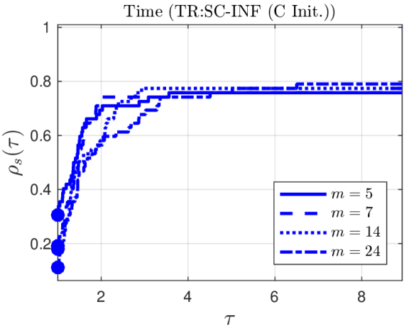
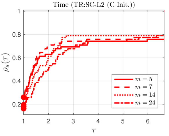
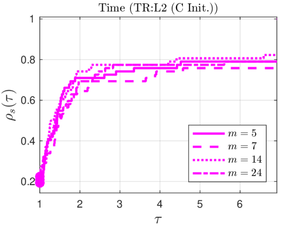
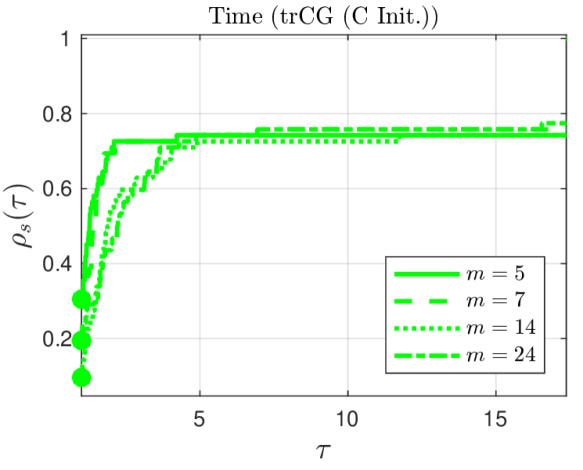
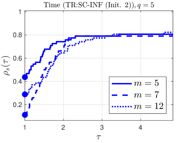
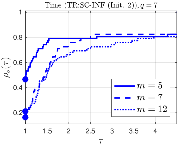
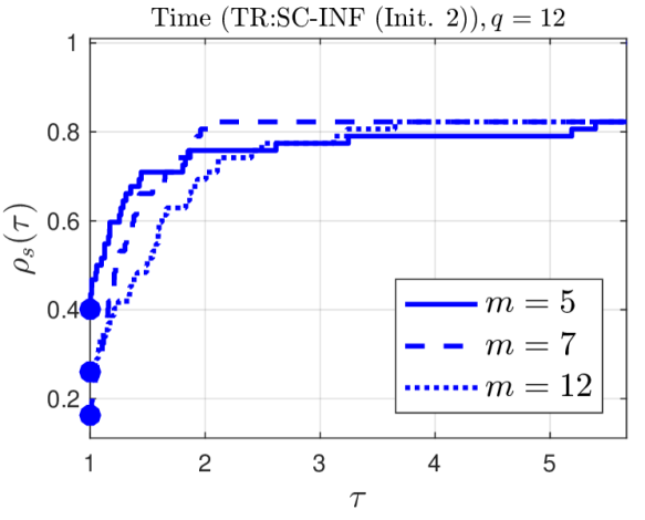
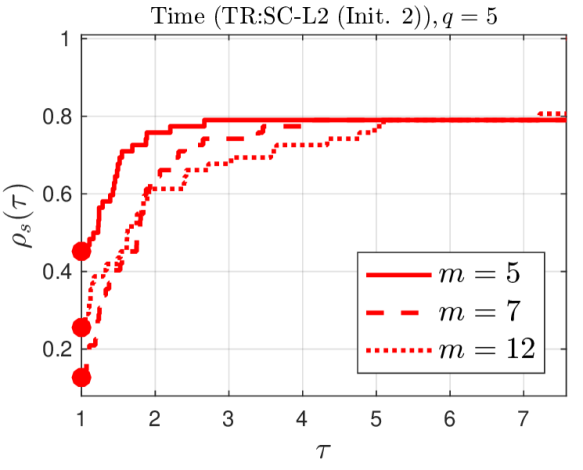
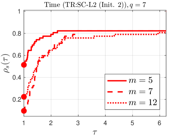
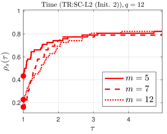
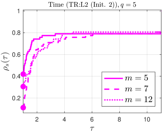
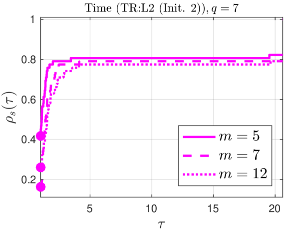
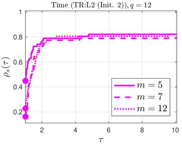
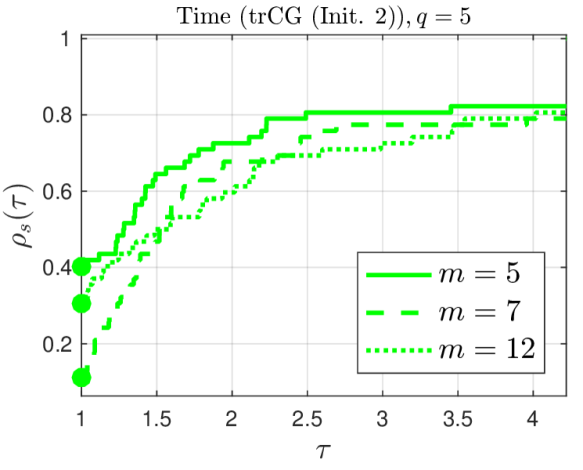
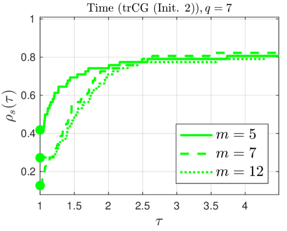
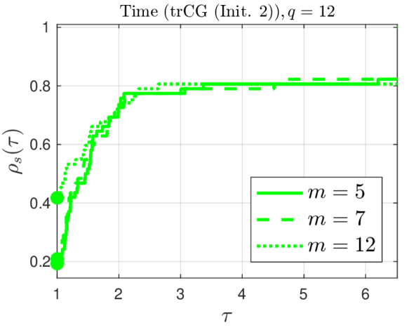
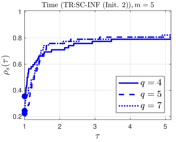
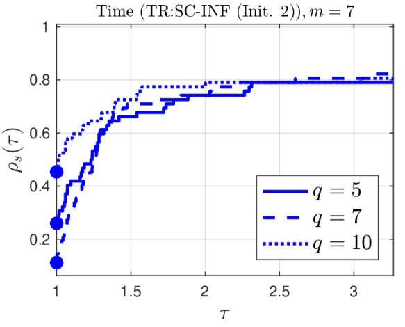
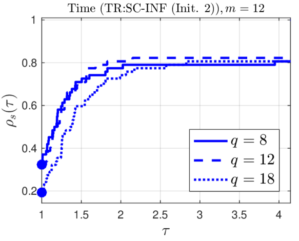
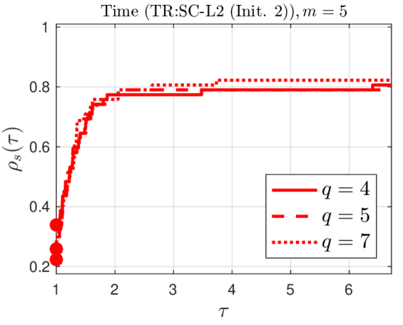
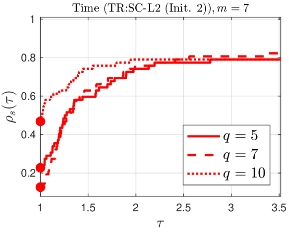
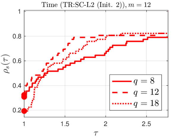
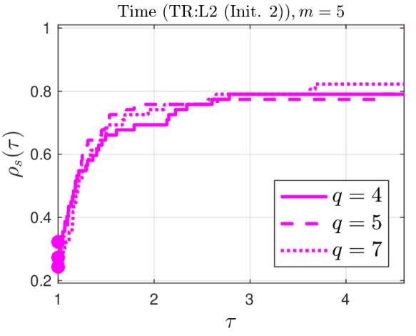
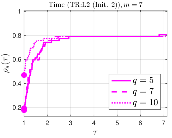
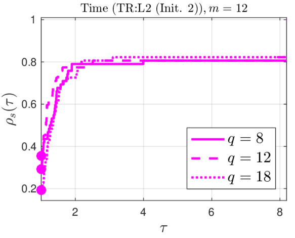
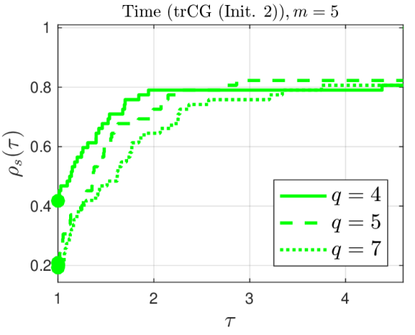
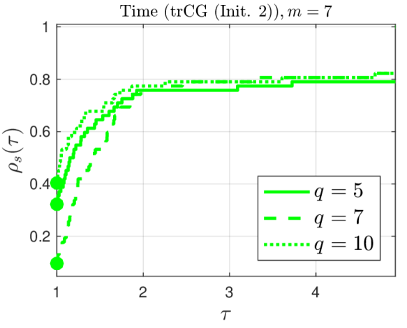
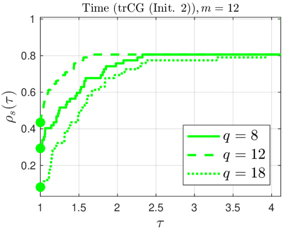
Initially, we included a $5^{\textnormal{th}}$ algorithm, LSTRS [36], which performed markedly inferior to any of the above solvers and is thus not reported as part of the outcomes in this section. We also found that Init. 2 performed significantly better than Init. 1, and therefore report the outcomes with Init. 2 below. Because the limited-memory updating mechanism is different whether a constant or non-constant initialization strategy is used, we describe our results separately for C Init. and Init. 2. As part of our comparisons we first select the best algorithm using only C Init. and only using Init. 2. Subsequently, we compare the best algorithms to each other. In order to find default parameters for our best algorithms, Figures 4, 5, and 6 report results for a considerable range of $m$ and $q$ values.

All remaining experiments are for the general unconstrained minimization problem

$$\underset{\mathbf{x}\in\mathbb{R}^{n}}{\text{ minimize }}f(\mathbf{x}),$$ (43)

where $f:\mathbb{R}^{n}\to\mathbb{R}$. We consider this problem solved once $\|\nabla f(\mathbf{x}_{k})\|_{\infty}\leq\varepsilon$. Our convergence tolerance is set to be $\varepsilon=5\times 10^{-4}$. With $\gamma$ fixed, a L-SR1 algorithm can be implemented by only storing the matrices $\mathbf{\Psi}_{k}$ and $\mathbf{M}_{k}^{-1}$. In particular, with a fixed $\gamma=\gamma_{k}$ in (4) then $\mathbf{M}_{k}^{-1}\mathbf{e}_{k}=\mathbf{\Psi}^{T}_{k}\mathbf{s}_{k}$, so that updating the symmetric matrix $\mathbf{M}_{k}^{-1}$ only uses $O(nm)$ multiplications. In this way, the overall computational complexity and memory requirements of the L-SR1 method are reduced as compared to non-constant initializations. However, using a non-constant initialization strategy can adaptively incorporate additional information, which can be advantageous. Therefore, we compare the best algorithms for constant and non-constant initialization strategies in Sections 5.4, 5.5 and 5.6. Parameters in Algorithm 5 are set as follows: $c_{1}=9\times 10^{-4}$, $c_{2}=0.75$, $c_{3}=0.8$, $c_{4}=2$, $c_{5}=0.1$, $c_{6}=0.75$, $c_{7}=0.5$ and $\varepsilon_{\text{SR1}}=1\times 10^{-8}$.

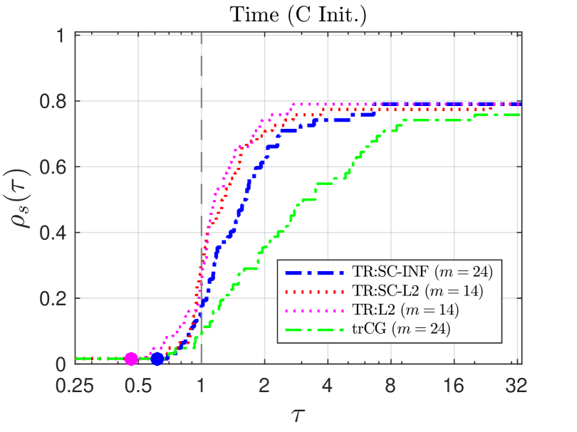
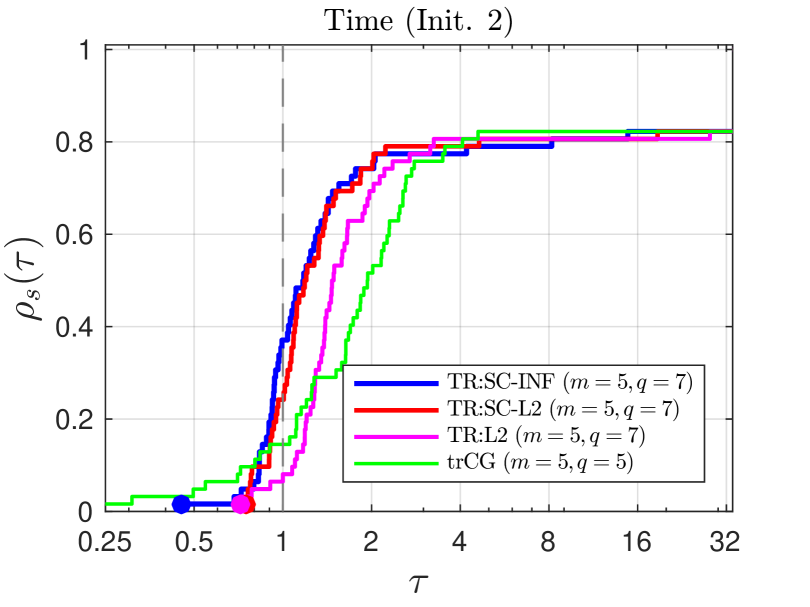
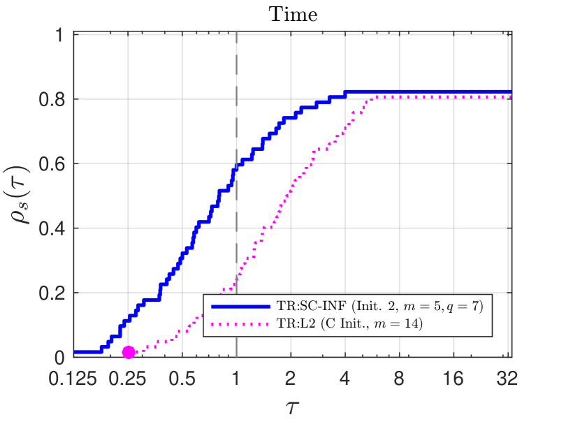
Extended performance profiles as in [37] are provided. These profiles are an extension of the well known profiles of Dolan and Moré [38]. We compare total computational time for each solver on the test set of problems. The performance metric $\rho_{s}(\tau)$ with a given number of test problems $n_{p}$ is

$$\rho_{s}(\tau)=\frac{\text{card}\left\{p:\pi_{p,s}\leq\tau\right\}}{n_{p}}\quad\text{and}\quad\pi_{p,s}=\frac{t_{p,s}}{\underset{1\leq i\leq S,i\neq s}{\text{ min }t_{p,i}}},$$

where $t_{p,s}$ is the “output” (i.e., time) of “solver” $s$ on problem $p$. Here $S$ denotes the total number of solvers for a given comparison. This metric measures the proportion of how close a given solver is to the best result. The extended performance profiles are the same as the classical ones for $\tau\geq 1$. In the profiles we include a dashed vertical grey line, to indicate $\tau=1$. The solvers are compared on 62 large-scale CUTEst problems, which are the same problems as in [2]. Additionally, Appendix A.3 includes supplementary comparisons on quadratics and the Rosenbrock objectives.

5.4. Comparisons with constant initialization strategy (C Init.)

This experiment compares the algorithms when the constant initialization C Init. from (40) is used. Because the memory allocation is essentially halved (relative to a non-constant initialization) the memory parameter $m$ includes larger values, too (such as $m=24$). For each individual solver we first determine its optimal $m$ parameter in Figure 4. After selecting the best parameters, these best solvers are then compared in Figure 1.

Figure 1. Comparison of best algorithms with C Init. (constant initialization), which are selected from Figure 4. Observe that TR:L2 obtains the best results in this comparison. The limited-memory parameter $m$ is relatively large for all solvers, however since a constant initialization is used larger memory values are permissible.

5.5. Comparisons with non-constant initialization strategy (Init. 2)

Since Init. 2 depends on the parameter $q$, Figures 5 and 6 test each algorithm on a combination of $m$ and $q$ values. A comparison of the best values for each algorithm is in Figure 2.

Figure 2. Comparison of best algorithms with Init.2 (non-constant initialization), which are selected as the best ones from Figures 5, and 6. Observe that TR:SC-INF and TR:SC-L2 obtain the overall best results. All algorithms use a small memory parameter $m=5$. Since Init. 2 is a non-constant initialization these algorithms store $\mathbf{S}_{k},\mathbf{Y}_{k}$ to implicitly represent $\boldsymbol{\Psi}_{k}$, and thus the memory allocations scale with $2\cdot m$.

5.6. Comparisons of best outcomes

The overall best algorithms from Figures 1 and 2 are compared in Figure 3. This declares that the best performing algorithm over the sequence of experiments is TR:SC-INF with the indicated parameter values.

Figure 3. Overall comparison of best algorithms by selecting winners in Figures 1 (C Init.) and 2 (Init. 2). Observe that TR:SC-INF with non-constant initialization strategy outperforms the best algorithm with a constant initialization (TR:L2). In sum, the trust-region algorithm with the proposed shape-changing infinity subproblem solver (TR:SC-INF) obtains the best results among the comparisons on 62 large-scale CUTEst problems.

6. Concluding remarks

In this paper, we presented a high-accuracy trust-region subproblem solver for when the Hessian is approximated by L-SR1 matrices. The method makes use of special shape-changing norms that decouple the original subproblem into two separate subproblems. Numerical experiments using the $(\mathbf{P},2)$ norm verify that solutions are computed to high accuracy in cases when there are no closed-form solutions and also in the so-called “hard case”. Experiments on large-scale unconstrained optimization problems demonstrate that the proposed algorithms perform well when compared to widely used methods, such as truncated CG or an $\ell_{2}$ TR subproblem algorithm.

APPENDIX

This appendix lists our implementation of the L-SR1 trust-region algorithm from the numerical experiments in Section 5.3. This trust-region algorithm uses the trust-region radius adjustments from [19, Algorithm 6.2] and the subproblem solvers in Algorithms 3 and 4, as well as the orthonormal basis method (OBS) from [10].

  ALGORITHM 5: L-SR1 Shape-Changing Trust-Region Algorithms (LSR1_SC)  

0:  [$\mathbf{x}_{k},\mathbf{g}_{k},f_{k},\text{out}$]=LSR1_SC($\mathbf{x}$, $f(\mathbf{x})$, $\nabla f(\mathbf{x})$, pars)

1:  Set constants from pars: $0<c_{1}<1\times 10^{-3}$, $0<c_{2}$, $0<c_{3}<1$, $1<c_{4}$, $0<c_{5}\leq c_{2}$, $0<c_{6}<1$, $0<c_{7}<1$,$0<\varepsilon$, $0<m$, $0<q$, $0<\varepsilon_{\text{SR1}}$, $\text{ALG}\leftarrow\text{pars.whichSub}$, $\text{INIT}\leftarrow\text{pars.whichInit}$, $\text{SAVE}\leftarrow\text{pars.storePsiPsi}$, ;

2:  Initialize $k\leftarrow 0$, $k_{m}\leftarrow 0$, $\mathbf{x}_{k}\leftarrow\mathbf{x}$, $0<\gamma_{k}$, $0<\gamma_{\text{max}}$, $\text{inv}\mathbf{M}_{k}\leftarrow[]$, $\text{mIdx}\leftarrow 1:m$, $\text{iEx}\leftarrow 0$;

3:  $f_{k}\leftarrow f(\mathbf{x}_{k})$, $\mathbf{g}_{k}\leftarrow\nabla f(\mathbf{x}_{k})$;

4:  $[\mathbf{x}_{k+1},\mathbf{g}_{k+1},f_{k+1}]\leftarrow\text{lineSearch}(\mathbf{x}_{k},\mathbf{g}_{k},f_{k})$;

5:  $\mathbf{s}_{k}\leftarrow\mathbf{x}_{k+1}-\mathbf{x}_{k},\mathbf{y}_{k}\leftarrow\mathbf{g}_{k+1}-\mathbf{g}_{k}$;

6:  if $\text{INIT}=\text{C.Init.}$ then

7:     % Constant initialization

8:     $\gamma_{k}\leftarrow\text{max}(\text{min}(\|\mathbf{y}_{0}\|^{2}/\mathbf{s}^{T}_{0}\mathbf{y}_{0},\gamma_{\text{max}}),1)$

9:     $\mathbf{\Psi}_{k}\leftarrow[]$;

10:  else

11:     % Non-constant initialization.

12:     $\gamma_{k}\leftarrow\|\mathbf{y}_{k}\|^{2}/\mathbf{s}^{T}_{k}\mathbf{y}_{k}$;

13:     $\mathbf{S}_{k}\leftarrow[]$, $\mathbf{Y}_{k}\leftarrow[]$, $\mathbf{D}_{k}\leftarrow[]$, $\mathbf{L}_{k}\leftarrow[]$, $\mathbf{T}_{k}\leftarrow[]$, $\mathbf{SS}_{k}\leftarrow[]$, $\mathbf{YY}_{k}\leftarrow[]$;

14:  end if

15:  if $\text{SAVE}=1$ then

16:     $\boldsymbol{\Psi}\boldsymbol{\Psi}_{k}\leftarrow[]$;

17:  end if

18:  $b_{k}\leftarrow\mathbf{s}^{T}_{k}(\mathbf{y}_{k}-\gamma_{k}\mathbf{s}_{k})$;

19:  if  $\varepsilon_{\text{SR1}}{\color[rgb]{0,0,0}\|\mathbf{s}_{k}\|_{2}\|\mathbf{y}_{k}-\gamma_{k}\mathbf{s}_{k}\|_{2}}<\text{abs}(b_{k})$ then

20:     $k_{m}\leftarrow k_{m}+1$;

21:     $\text{inv}\mathbf{M}_{k}(k_{m},k_{m})\leftarrow b_{k}$;

22:     if $\text{INIT}=\text{C.Init.}$ then

23:        $[\boldsymbol{\Psi}_{k},\text{mIdx}]=\texttt{colUpdate}(\boldsymbol{\Psi}_{k},\mathbf{y}_{k}-\gamma_{k}\mathbf{s}_{k},\text{mIdx},m,k)$ % From Procedure 1

24:     else

25:        $[\mathbf{Y}_{k},\sim]=\texttt{colUpdate}(\mathbf{Y}_{k},\mathbf{y}_{k},\text{mIdx},m,k)$;

26:        $[\mathbf{S}_{k},\text{mIdx}]=\texttt{colUpdate}(\mathbf{S}_{k},\mathbf{s}_{k},\text{mIdx},m,k)$;

27:        $\mathbf{D}_{k}(k_{m},k_{m})=\mathbf{s}_{k}^{T}\mathbf{y}_{k}$;

28:        $\mathbf{L}_{k}(k_{m},k_{m})=\mathbf{s}_{k}^{T}\mathbf{y}_{k}$;

29:        $\mathbf{T}_{k}(k_{m},k_{m})=\mathbf{s}_{k}^{T}\mathbf{y}_{k}$;

30:        $\mathbf{SS}_{k}(k_{m},k_{m})=\mathbf{s}_{k}^{T}\mathbf{s}_{k}$;

31:        $\mathbf{YY}_{k}(k_{m},k_{m})=\mathbf{y}_{k}^{T}\mathbf{y}_{k}$;

32:     end if

33:  end if

34:  $\delta_{k}\leftarrow 2\|\mathbf{s}_{k}\|$;

35:  $k\leftarrow k+1$;

36:  while ($\varepsilon\leq\|\mathbf{g}_{k}\|_{2}$) and ($k\leq\text{maxIt}$)  do

37:     Choose TR subproblem solver to compute $\mathbf{s}_{k}$ (E.g., Alg. 3, Alg. 4, $\ell_{2}$-norm, truncated CG);

38:     % For example: sc_sr1_infty with $\Psi^{T}\Psi$ updating

39:      $\mathbf{s}_{k}\leftarrow$ sc_sr1_infty($\mathbf{g}_{k}$,$\mathbf{S}_{k}(:,\text{mIdx}(1:k_{m}))$, $\mathbf{Y}_{k}(:,\text{mIdx}(1:k_{m}))$, $\gamma_{k}$, $\delta_{k}$, $1$, $0$, $\ldots$$\boldsymbol{\Psi\Psi}_{k}(1:k_{m},1:k_{m})$,$\text{inv}\mathbf{M}_{k}(1:k_{m},1:k_{m})$);

40:     $\widehat{\mathbf{x}}_{k+1}\leftarrow\mathbf{x}_{k}+\mathbf{s}_{k},\widehat{f}_{k+1}\leftarrow f(\widehat{\mathbf{x}}_{k+1}),\widehat{\mathbf{g}}_{k+1}\leftarrow\nabla f(\widehat{\mathbf{x}}_{k+1})$;

41:     if $\text{INIT}=\text{C.Init}$ then

42:        $\mathbf{b}_{k}(1:k_{m})\leftarrow\mathbf{\Psi}_{k}(:,\text{mIdx}(1:k_{m}))^{T}\mathbf{s}_{k}$;

43:     else

44:        % Non-constant initialization, stores additionally $\mathbf{b1}_{k},\mathbf{b2}_{k}$

45:        $\mathbf{b1}_{k}(1:k_{m})\leftarrow\mathbf{Y}_{k}(:,\text{mIdx}(1:k_{m}))^{T}\mathbf{s}_{k}$;

46:        $\mathbf{b2}_{k}(1:k_{m})\leftarrow\mathbf{S}_{k}(:,\text{mIdx}(1:k_{m}))^{T}\mathbf{s}_{k}$;

47:        $\mathbf{b}_{k}(1:k_{m})\leftarrow\mathbf{b1}_{k}(1:k_{m})-\gamma_{k}\mathbf{b2}_{k}(1:k_{m})$;

48:     end if

49:     $(sBs)_{k}\leftarrow\gamma_{k}\mathbf{s}^{T}_{k}\mathbf{s}_{k}+\frac{1}{2}\mathbf{b}_{k}(1:k_{m})^{T}(\text{inv}\mathbf{M}_{k}(1:k_{m},1:k_{m})\backslash\mathbf{b}_{k}(1:k_{m}))$;

50:     if $\textnormal{INIT}=\textnormal{Init. 2}$ then

51:        % Other non-constant initialization strategies can be implemented here

52:        $\gamma_{k}\leftarrow\text{max}(\|\mathbf{y}_{k-q}\|^{2}/\mathbf{s}^{T}_{k-q}\mathbf{y}_{k-q},\cdots,\|\mathbf{y}_{k}\|^{2}/\mathbf{y}_{k}^{T}\mathbf{s}_{k})$

53:     end if

54:     $\rho_{k}\leftarrow\frac{\widehat{f}_{k+1}-f_{k}}{\mathbf{s}^{T}_{k}\mathbf{g}_{k}+(sBs)_{k}}$;

55:     if $c_{1}<\rho_{k}$ then

56:        $\mathbf{x}_{k+1}\leftarrow\widehat{\mathbf{x}}_{k+1}$;

57:        $\mathbf{g}_{k+1}\leftarrow\widehat{\mathbf{g}}_{k+1}$;

58:        $f_{k+1}\leftarrow\widehat{f}_{k+1}$;

59:     else

60:        $\mathbf{x}_{k+1}\leftarrow\mathbf{x}_{k}$;

61:     end if

62:     if $c_{2}<\rho_{k}$ then

63:        if $\|\mathbf{s}_{k}\|_{2}\leq c_{3}\delta_{k}$ then

64:           $\delta_{k}\leftarrow\delta_{k}$;

65:        else

66:           $\delta_{k}\leftarrow c_{4}\delta_{k}$;

67:        end if

68:     else if $c_{5}\leq\rho_{k}\leq c_{6}$ then

69:        $\delta_{k}\leftarrow\delta_{k}$;

70:     else

71:        $\delta_{k}\leftarrow c_{7}\delta_{k}$;

72:     end if

73:     $\mathbf{y}_{k}\leftarrow\widehat{\mathbf{g}}_{k+1}-\mathbf{g}_{k}$;

74:     $b_{k}\leftarrow\mathbf{s}_{k}^{T}\mathbf{y}_{k}+(sBs)_{k}$;

75:     if $\varepsilon_{\text{SR1}}{\color[rgb]{0,0,0}\|\mathbf{s}_{k}\|_{2}\|\mathbf{y}_{k}-\gamma_{k}\mathbf{s}_{k}\|_{2}}\leq\text{abs}(b_{k})$ then

76:        if $\text{INIT}=\text{C.Init.}$ then

77:           $[\boldsymbol{\Psi}_{k},\text{mIdx}]=\texttt{colUpdate}(\boldsymbol{\Psi}_{k},\mathbf{y}_{k}-\gamma_{k}\mathbf{s}_{k},\text{mIdx},m,k)$;

78:           if ($k_{m}<m$) then

79:              $k_{m}\leftarrow k_{m}+1$;

80:           end if

81:           $\text{inv}\mathbf{M}_{k}(1:(k_{m}-1),k_{m})\leftarrow\mathbf{b}_{k}(1:(k_{m}-1))$;

82:           $\text{inv}\mathbf{M}_{k}(k_{m},1:(k_{m}-1))\leftarrow\mathbf{b}_{k}(1:(k_{m}-1))$;

83:           $\text{inv}\mathbf{M}_{k}(k_{m},k_{m})\leftarrow b_{k}$;

84:           if $\textnormal{SAVE}=1$ then

85:              % Update and store the product $\Psi_{k}^{T}\Psi_{k}$

86:              $\boldsymbol{\Psi\Psi}_{k}(1:k_{m},1:k_{m})=\texttt{prodUpdate}(\boldsymbol{\Psi\Psi}_{k},\boldsymbol{\Psi}_{k},\boldsymbol{\Psi}_{k},\mathbf{y}_{k}-\gamma_{k}\mathbf{s}_{k},\mathbf{y}_{k}-\gamma_{k}\mathbf{s}_{k},\text{mIdx},m,k)$;

87:           end if

88:        else

89:           % Non-constant initialization

90:           $[\mathbf{Y}_{k},\sim]=\texttt{colUpdate}(\mathbf{Y}_{k},\mathbf{y}_{k},\text{mIdx},m,k)$;

91:           $[\mathbf{S}_{k},\text{mIdx}]=\texttt{colUpdate}(\mathbf{S}_{k},\mathbf{s}_{k},\text{mIdx},m,k)$;

92:           $\mathbf{T}_{k}=\texttt{prodUpdate}(\mathbf{T}_{k},\mathbf{S}_{k},0,\mathbf{s}_{k},\mathbf{y}_{k},\text{mIdx},m,k)$;

93:           $\mathbf{YY}_{k}=\texttt{prodUpdate}(\mathbf{YY}_{k},\mathbf{Y}_{k},\mathbf{Y}_{k},\mathbf{y}_{k},\mathbf{y}_{k},\text{mIdx},m,k)$;

94:           if ($k_{m}<m$) then

95:              $k_{m}\leftarrow k_{m}+1$;

96:           end if

97:           $\mathbf{D}_{k}(k_{m},k_{m})\leftarrow\mathbf{s}_{k}^{T}\mathbf{y}_{k}$;

98:           $\mathbf{L}_{k}(k_{m},1:(k_{m}-1))\leftarrow\mathbf{b1}_{k}(1:(k_{m}-1))$;

99:           $\mathbf{SS}_{k}(1:(k_{m}-1),k_{m})\leftarrow\mathbf{b2}_{k}(1:(k_{m}-1))$;

100:           $\mathbf{SS}_{k}(k_{m},1:(k_{m}-1))\leftarrow\mathbf{b2}_{k}(1:(k_{m}-1))$;

101:           $\mathbf{SS}_{k}(k_{m},k_{m})\leftarrow\mathbf{s}_{k}^{T}\mathbf{s}_{k}$;

102:           $\text{inv}\mathbf{M}_{k}(1:k_{m},1:k_{m})\leftarrow\mathbf{D}_{k}(1:k_{m},1:k_{m})+\mathbf{L}_{k}(1:k_{m},1:k_{m})+\mathbf{L}_{k}(1:k_{m},1:k_{m})^{T}-\gamma_{k}\mathbf{SS}_{k}(1:k_{m},1:k_{m})$;

103:           if $\textnormal{SAVE}=1$ then

104:              % Update and store the product $\Psi_{k}^{T}\Psi_{k}$ with non-constant initialization

105:              $\boldsymbol{\Psi\Psi}_{k}(1:k_{m},1:k_{m})=\mathbf{YY}_{k}(1:k_{m},1:k_{m})-\gamma_{k}(\mathbf{T}_{k}(1:k_{m},1:k_{m})+\mathbf{T}_{k}(1:k_{m},1:k_{m})^{T}+\mathbf{L}_{k}(1:k_{m},1:k_{m})+\mathbf{L}_{k}(1:k_{m},1:k_{m})^{T})+\gamma_{k}^{2}\mathbf{SS}_{k}(1:k_{m},1:k_{m})$;

106:           end if

107:        end if

108:     end if

109:     $\mathbf{x}_{k}\leftarrow\mathbf{x}_{k+1}$, $\mathbf{g}_{k}\leftarrow\mathbf{g}_{k+1}$, $f_{k}\leftarrow f_{k+1}$, $k\leftarrow k+1$;

110:  end while

111:  $\text{out.numiter}\leftarrow k,\text{out.ng}\leftarrow\|\mathbf{g}_{k}\|$;

112:  return  $\mathbf{x}_{k},\mathbf{g}_{k},f_{k},\text{out}$

 

A.1. Experiments to determine default parameters with constant Initialization (C Init.)

Figure 4. Comparison of the computational times for the 4 algorithms $\{\textnormal{TR:SC-INF, TR:SC-L2, TR:L2, trCG}\}$ when a constant initialization (C Init.) is used, and the limited memory parameter is $m=[5,7,14,24]$.

A.2. Experiments to determine default parameters with non-constant Initialization (Init. 2)

Figure 5. Comparison of the computational times for the 4 algorithms $\{\textnormal{TR:SC-INF, TR:SC-L2, TR:L2, trCG}\}$ when the non-constant initialization (Init. 2) is used, and the parameters are $q=[5,7,12]$ and $m=[5,7,12]$.

Figure 6. Comparison of the computational times for the 4 algorithms $\{\textnormal{TR:SC-INF, TR:SC-L2, TR:L2, trCG}\}$ when the non-constant initialization (Init. 2) is used, and the parameters are $m=[5,7,12]$ and $q=[\texttt{ceil}(2/3\cdot m_{i}),m_{i},\texttt{floor}(3/2\cdot m_{i})],1\leq i\leq 3$.

A.3. Experiments on quadratics and the Rosenbrock functions

In this set of experiments we vary the problem dimension as $n=[5\times 10^{2},1\times 10^{3},5\times 10^{3},1\times 10^{4},5\times 10^{4},1\times 10^{5},3\times 10^{5}]$, set the memory parameter $m=5$, use Init. 2 for all solvers and set the maximum iterations as $\text{maxIt}=500$. In Table VIII, we let $f(\mathbf{x})$ be the Rosenbrock function defined by $f(\mathbf{x})=\sum_{i=1}^{n}(\mathbf{x}_{2i}-\mathbf{x}^{2}_{2i-1})^{2}+(1-\mathbf{x}^{2}_{2i-1})^{2}$. We initialize the trust-region algorithm (Algorithm 5) from the starting point $[\mathbf{x}_{0}]_{1}=30,[\mathbf{x}_{0}]_{2:n}=0$. (With this initial point the gradient norm $\|\nabla f(\mathbf{x}_{0})\|_{2}\approx 10^{5}$). Table VIII reports the outcomes of using the trust-region algorithm with these three different subproblem solvers.

Table 8. Results of solving problem (43) with the Rosenbrock objective function. The maximum number of iterations are: $\text{maxIt}=500$ and the convergence tolerance is $\|\nabla f(\mathbf{x}_{k})\|_{\infty}\leq 1\times 10^{-4}$. The memory parameter is $m=5$. The column nA denotes the number of “accepted” search directions, which corresponds to line 55 in Algorithm 5 being true. Observe that all algorithms converged to the prescribed tolerances on all problem instances.

$n$	TR:SC-INF (Alg. 3)				TR:SC-L2 (Alg. 4)				TR-L2
	$k$	nA	Time	$\|\nabla f(\mathbf{x}_{k})\|$	$k$	nA	Time	$\|\nabla f(\mathbf{x}_{k})\|$	$k$	nA	Time	$\|\nabla f(\mathbf{x}_{k})\|$
$5\times 10^{2}$	40	26	2.00e-02	7.18e-05	46	29	1.59e-02	3.11e-05	36	24	1.34e-02	2.89e-06
$1\times 10^{3}$	38	24	1.13e-02	2.23e-05	41	24	1.28e-02	3.83e-05	32	22	1.14e-02	2.02e-05
$5\times 10^{3}$	42	31	3.02e-02	1.17e-05	38	29	2.75e-02	6.38e-05	43	26	4.26e-02	5.03e-05
$1\times 10^{4}$	46	30	5.22e-02	4.57e-07	40	28	4.20e-02	5.80e-05	48	29	6.30e-02	8.87e-05
$5\times 10^{4}$	47	33	2.14e-01	1.01e-06	39	28	1.73e-01	1.22e-05	54	35	2.85e-01	6.92e-05
$1\times 10^{5}$	40	31	3.94e-01	6.82e-05	58	39	4.81e-01	1.06e-05	44	27	4.97e-01	1.57e-08
$3\times 10^{5}$	60	39	2.74e+00	1.63e-06	53	33	2.49e+00	3.52e-06	68	43	3.53e+00	1.70e-05

In table IX, we let $f(\mathbf{x})$ be quadratic functions defined by $f(\mathbf{x})=\mathbf{g}^{T}\mathbf{x}+\frac{1}{2}(\mathbf{x}^{T}(\phi\mathbf{I}+\mathbf{Q}\mathbf{D}\mathbf{Q}^{T})\mathbf{x})$. In particular, we let $\mathbf{Q}\in\mathbb{R}^{n\times r}$ be a rectangular matrix and $\mathbf{D}\in\mathbb{R}^{r\times r}$ be a diagonal matrix. We initialize the trust-region algorithm (Algorithm 5) from the starting point $\mathbf{x}_{0}=\mathbf{0}$. We generate $\mathbf{Q}=\texttt{rand}(n,r)$, $\mathbf{D}=\text{diag}(\texttt{rand}(r,1))$ and $\mathbf{g}=\texttt{randn}(n,1)$, after initializing the random number generator by the command $\texttt{rng}(\texttt{`default'})$. Moreover, we set $r=10$, $\phi=100$ and the maximum number of iterations as $\text{maxIt}=500$. All other parameters of the method are as before. Table IX reports the outcomes of using the trust-region algorithm with the three different subproblem solvers.

Table 9. Results of solving problem (43) with quadratic objective functions. The maximum number of iterations are set as $\text{maxIt}=500$ and the convergence tolerance $\|\nabla f(\mathbf{x}_{k})\|_{\infty}\leq 1\times 10^{-4}$. The memory parameter is $m=5$. The column nA denotes the number of “accepted” search directions (line 55 in Algorithm 5 is true). Observe that Alg. 3 and Alg. 4 converged on all problems. Moreover, Alg. 3 and Alg. 4 were fastest on the on the largest two problem instances.

$n$	TR:SC-INF (Alg. 3)				TR:SC-L2 (Alg. 4)				TR:L2 ($\ell_{2}$ [10])
	$k$	nA	Time	$\|\nabla f(\mathbf{x}_{k})\|$	$k$	nA	Time	$\|\nabla f(\mathbf{x}_{k})\|$	$k$	nA	Time	$\|\nabla f(\mathbf{x}_{k})\|$
$5\times 10^{2}$	8	6	5.75e-02	6.56e-06	8	6	2.66e-02	6.56e-06	6	4	2.89e-02	8.03e-06
$1\times 10^{3}$	8	6	7.25e-03	4.06e-05	8	6	7.51e-03	4.06e-05	6	4	6.67e-03	5.11e-05
$5\times 10^{3}$	21	15	2.47e-02	8.96e-05	21	15	2.83e-02	9.14e-05	16	10	2.79e-02	3.71e-05
$1\times 10^{4}$	23	18	3.86e-02	7.79e-05	23	18	3.65e-02	5.21e-05	19	14	3.65e-02	4.28e-05
$5\times 10^{4}$	45	33	2.16e-01	1.58e-05	60	46	2.28e-01	9.71e-05	27	21	1.20e-01	9.13e-05
$1\times 10^{5}$	62	49	5.04e-01	9.80e-05	79	64	5.86e-01	9.72e-05	500	494	4.05e+00	4.09e-04
$3\times 10^{5}$	20	15	8.99e-01	3.49e-05	22	17	8.37e-01	3.86e-05	26	17	1.11e+00	9.97e-05

Remarkably, observe in the outcomes of Tables VIII and IX that a limited memory trust-region algorithm using our subproblem solvers is able to solve large optimization problems, with $n\approx 1\times 10^{5}$, within seconds. Moreover, we observe that the proposed algorithms (Algorithm 3 and Algorithm 4) may require fewer iterations on some problems than a $\ell_{2}$-norm method and use less computational time. Future research, can investigate the effectiveness of a L-SR1 trust-region algorithm for non-convex objective functions and improve on the efficiency of the implementation.

References

- [1] O. Burdakov and Y.-X. Yuan. On limited-memory methods with shape changing trust region. In Proceedings of the First International Conference on Optimization Methods and Software, page p. 21, 2002.
- [2] Oleg Burdakov, Lujin Gong, Spartak Zikrin, and Ya-xiang Yuan. On efficiently combining limited-memory and trust-region techniques. Mathematical Programming Computation, 9(1):101–134, 2017.
- [3] D. M. Gay. Computing optimal locally constrained steps. SIAM J. Sci. Statist. Comput., 2(2):186–197, 1981.
- [4] J. J. Moré and D. C. Sorensen. Computing a trust region step. SIAM J. Sci. and Statist. Comput., 4:553–572, 1983.
- [5] D. C. Sorensen. Newton’s method with a model trust region modification. SIAM J. Numer. Anal., 19(2):409–426, 1982.
- [6] J. B. Erway and P. E. Gill. A subspace minimization method for the trust-region step. SIAM Journal on Optimization, 20(3):1439–1461, 2010.
- [7] J. B. Erway, P. E. Gill, and J. D. Griffin. Iterative methods for finding a trust-region step. SIAM Journal on Optimization, 20(2):1110–1131, 2009.
- [8] J. B. Erway and R. F. Marcia. Algorithm 943: MSS: MATLAB software for L-BFGS trust-region subproblems for large-scale optimization. ACM Transactions on Mathematical Software, 40(4):28:1–28:12, June 2014.
- [9] N. I. M. Gould, D. P. Robinson, and H. S. Thorne. On solving trust-region and other regularised subproblems in optimization. Mathematical Programming Computation, 2(1):21–57, 2010.
- [10] J. J. Brust, J. B. Erway, and R. F. Marcia. On solving L-SR1 trust-region subproblems. Computational Optimization and Applications, 66(2):245–266, 2017.
- [11] K. G. Murty and S. N. Kabadi. Some np-complete problems in quadratic and nonlinear programming. Mathematical Programming, 39(2):117–129, 1987.
- [12] B. Vavasis. Nonlinear Optimization: Complexity Issues. International Series of Monographs on Computer Science. Oxford University Press, Oxford, England, 1992.
- [13] A. R. Conn, N. I. M. Gould, and P. L. Toint. Trust-Region Methods. Society for Industrial and Applied Mathematics (SIAM), Philadelphia, PA, 2000.
- [14] D. Goldfarb. The use of negative curvature in minimization algorithms. Technical Report 80-412, Cornell University, 1980.
- [15] T. Steihaug. The conjugate gradient method and trust regions in large scale optimization. SIAM J. Numer. Anal., 20:626–637, 1983.
- [16] O. Burdakov, S. Gratton, Y.-X Yuan, and S. Zikrin. LMTR suite for unconstrained optimization. http://gratton.perso.enseeiht.fr/LBFGS/index.html, 2018.
- [17] N. I. M. Gould, D. Orban, and P. L. Toint. CUTEr and SifDec: A constrained and unconstrained testing environment, revisited. ACM Trans. Math. Software, 29(4):373–394, 2003.
- [18] R. H. Byrd, J. Nocedal, and R. B. Schnabel. Representations of quasi-Newton matrices and their use in limited-memory methods. Math. Program., 63:129–156, 1994.
- [19] J. Nocedal and S. J. Wright. Numerical Optimization. Springer, New York, 2nd edition, 2006.
- [20] A. R. Conn, N. I. M. Gould, and Ph. L. Toint. Convergence of quasi-Newton matrices generated by the symmetric rank one update. Math. Programming, 50(2, (Ser. A)):177–195, 1991.
- [21] I. Griva, S. G. Nash, and A. Sofer. Linear and nonlinear programming. Society for Industrial and Applied Mathematics, Philadelphia, 2009.
- [22] C. T. Kelley and E. W. Sachs. Local convergence of the symmetric rank-one iteration. Computational Optimization and Applications, 9(1):43–63, 1998.
- [23] H. Fayez Khalfan, R. H. Byrd, and R. B. Schnabel. A theoretical and experimental study of the symmetric rank-one update. SIAM Journal on Optimization, 3(1):1–24, 1993.
- [24] W. Sun and Y.-x. Yuan. Optimization theory and methods, volume 1 of Springer Optimization and Its Applications. Springer, New York, 2006. Nonlinear programming.
- [25] H. Wolkowicz. Measures for symmetric rank-one updates. Mathematics of Operations Research, 19(4):815–830, 1994.
- [26] J. B. Erway and R. F. Marcia. On efficiently computing the eigenvalues of limited-memory quasi-newton matrices. SIAM Journal on Matrix Analysis and Applications, 36(3):1338–1359, 2015.
- [27] J. J. Brust. Large-Scale Quasi-Newton Trust-Region Methods: High-Accuracy Solvers, Dense Initializations, and Extensions. PhD thesis, University of California, Merced, 2018. https://escholarship.org/uc/item/2bv922qk.
- [28] J J. Brust, R F. Marcia, and C G. Petra. Large-scale quasi-newton trust-region methods with low dimensional linear equality constraints. Computational Optimization and Applications, 74:669–701, 2019.
- [29] X. Lu. A study of the limited memory SR1 method in practice. PhD thesis, Department of Computer Science, University of Colorado at Boulder, 1996.
- [30] J.J. Brust, O. Burdakov, J.B. Erway, and R.F. Marcia. A dense initialization for limited-memory quasi-Newton methods. Computational Optimization and Applications, 74:121–142, 2019.
- [31] G. H. Golub and C. F. Van Loan. Matrix Computations. The Johns Hopkins University Press, Baltimore, Maryland, third edition, 1996.
- [32] J. Barzilai and J. Borwein. Two-point step size gradient methods. IMA Journal of Numerical Analysis, 8(1):141–148, 01 1988.
- [33] J. M. Bennett. Triangular factors of modified matrices. Numerische Mathematik, 7(3):217–221, 1965.
- [34] P. E. Gill, G. H. Golub, W. Murray, and M. A. Saunders. Methods for modifying matrix factorizations. Mathematics of Computation, 28(126):505–535, 1974.
- [35] J. Nocedal. Updating quasi-Newton matrices with limited storage. Math. Comput., 35:773–782, 1980.
- [36] M. Rojas, S.A. Santos, and D.C. Sorensen. Algorithm 873: Lstrs: Matlab software for large-scale trust-region subproblems and regularization. ACM Trans. Math. Software, 34(2):1–28, 2008.
- [37] A. Mahajan, S. Leyffer, and C. Kirches. Solving mixed-integer nonlinear programs by qp diving. Technical Report ANL/MCS-P2071-0312, Mathematics and Computer Science Division, Argonne National Laboratory, Lemont, IL, 2012.
- [38] E. Dolan and J.J Moré. Benchmarking optimization software with performance profiles. Mathematical Programming, 91:201–213, 2002.