The clustering of galaxies in the completed SDSS-III Baryon Oscillation Spectroscopic Survey: cosmological analysis of the DR12 galaxy sample
Abstract
We present cosmological results from the final galaxy clustering data set of the Baryon Oscillation Spectroscopic Survey, part of the Sloan Digital Sky Survey III. Our combined galaxy sample comprises 1.2 million massive galaxies over an effective area of 9329 deg2 and volume of 18.7 Gpc3, divided into three partially overlapping redshift slices centred at effective redshifts 0.38, 0.51, and 0.61. We measure the angular diameter distance and Hubble parameter from the baryon acoustic oscillation (BAO) method after applying reconstruction to reduce non-linear effects on the BAO feature. Using the anisotropic clustering of the pre-reconstruction density field, we measure the product from the Alcock-Paczynski (AP) effect and the growth of structure, quantified by , from redshift-space distortions (RSD). We combine individual measurements presented in seven companion papers into a set of consensus values and likelihoods, obtaining constraints that are tighter and more robust than those from any one method; in particular, the AP measurement from sub-BAO scales sharpens constraints from post-reconstruction BAO by breaking degeneracy between and . Combined with Planck 2015 cosmic microwave background measurements, our distance scale measurements simultaneously imply curvature and a dark energy equation of state parameter , in strong affirmation of the spatially flat cold dark matter model with a cosmological constant (CDM). Our RSD measurements of , at 6 per cent precision, are similarly consistent with this model. When combined with supernova Ia data, we find even for our most general dark energy model, in tension with some direct measurements. Adding extra relativistic species as a degree of freedom loosens the constraint only slightly, to . Assuming flat CDM we find and , and we find a 95% upper limit of 0.16 eV/ on the neutrino mass sum.
keywords:
cosmology: observations, distance scale, large-scale structure1 Department of Physics, Carnegie Mellon University, 5000 Forbes Avenue, Pittsburgh, PA 15213, USA
2 The McWilliams Center for Cosmology, Carnegie Mellon University, 5000 Forbes Ave., Pittsburgh, PA 15213, USA
3 Leibniz-Institut für Astrophysik Potsdam (AIP), An der Sternwarte 16, D-14482 Potsdam, Germany
4 Lawrence Berkeley National Laboratory, 1 Cyclotron Road, Berkeley, CA 94720, USA
5 Apache Point Observatory and New Mexico State University, P.O. Box 59, Sunspot, NM 88349, USA
6 Sternberg Astronomical Institute, Moscow State University, Universitetski pr. 13, 119992 Moscow, Russia
7 Center for Cosmology and Astro-Particle Physics, Ohio State University, Columbus, Ohio, USA
8 Department Physics and Astronomy, University of Utah, 115 S 1400 E, Salt Lake City, UT 84112, USA
9 National Optical Astronomy Observatory, 950 N Cherry Ave, Tucson, AZ 85719, USA
10 Department of Physics, Yale University, 260 Whitney Ave, New Haven, CT 06520, USA
11 Instituto de Física Teórica (UAM/CSIC), Universidad Autónoma de Madrid, Cantoblanco, E-28049 Madrid, Spain
12 Departamento de Física Teórica M8, Universidad Autónoma de Madrid, E-28049 Cantoblanco, Madrid, Spain
13 Institut de Ciències del Cosmos (ICCUB), Universitat de Barcelona (IEEC-UB), Martí i Franquès 1, E08028 Barcelona, Spain
14 Harvard-Smithsonian Center for Astrophysics, 60 Garden St., Cambridge, MA 02138, USA
15 CPPM, Aix-Marseille Université, CNRS/IN2P3, CPPM UMR 7346, 13288, Marseille, France
16 Sorbonne Universités, Institut Lagrange de Paris (ILP), 98 bis Boulevard Arago, 75014 Paris, France
17 Laboratoire de Physique Nucléaire et de Hautes Energies, Université Pierre et Marie Curie, 4 Place Jussieu, 75005 Paris, France
18 Universitäts-Sternwarte München, Scheinerstrasse 1, 81679 Munich, Germany
19 Max-Planck-Institut für Extraterrestrische Physik, Postfach 1312, Giessenbachstr., 85748 Garching, Germany
20 Department of Astronomy, University of California at Berkeley, Berkeley, CA 94720, USA
21 Department of Physics and Astronomy, UC Irvine, 4129 Frederick Reines Hall, Irvine, CA 92697, USA
22 Institute of Cosmology & Gravitation, Dennis Sciama Building, University of Portsmouth, Portsmouth, PO1 3FX, UK
23 Department of Chemistry and Physics, King’s College, 133 North River St, Wilkes Barre, PA 18711, USA
24 CEA, Centre de Saclay, IRFU/SPP, F-91191 Gif-sur-Yvette, France
25 Instituto de Astrofísica de Canarias (IAC), C/Vía Láctea, s/n, E-38200, La Laguna, Tenerife, Spain
26 Dpto. Astrofísica, Universidad de La Laguna (ULL), E-38206 La Laguna, Tenerife, Spain
27 Institut d’Astrophysique de Paris, Université Paris 6 et CNRS, 98bis Boulevard Arago, 75014 Paris, France
28 Campus of International Excellence UAM+CSIC, Cantoblanco, E-28049 Madrid, Spain
29 Instituto de Astrofísica de Andalucía (CSIC), E-18080 Granada, Spain
30 Department of Astrophysical Sciences, Princeton University, Ivy Lane, Princeton, NJ 08544, USA
31 Hubble Fellow
32 Department of Physics, University of California, 366 LeConte Hall, Berkeley, CA 94720, USA
33 Institute for Astronomy, University of Edinburgh, Royal Observatory, Edinburgh, EH9 3HJ, UK
34 Department of Astronomy and Space Science, Sejong University, Seoul 143-747, Korea
35 Kavli Institute for the Physics and Mathematics of the Universe (WPI), The University of Tokyo Institutes for Advanced Study, The University of Tokyo, Kashiwa, Chiba 277-8583, Japan
36 Max Planck Institut für Astrophysik, Karl-Schwarzschild-Straße 1, D-85740 Garching bei München, Germany
37 Department of Physics, Kansas State University, 116 Cardwell Hall, Manhattan, KS 66506, USA
38 Facultad de Ciencias Astronómicas y Geofísicas - Universidad Nacional de La Plata. Paseo del Bosque S/N, (1900) La Plata, Argentina
39 CONICET, Rivadavia 1917, (1033) Buenos Aires, Argentina
40 Department of Astronomy and Astrophysics, The Pennsylvania State University, University Park, PA 16802, USA
41 Institute for Gravitation and the Cosmos, The Pennsylvania State University, University Park, PA 16802, USA
42 Department of Physics and Astronomy, Ohio University, 251B Clippinger Labs, Athens, OH 45701, USA
43 Brookhaven National Laboratory, Bldg 510, Upton, New York 11973, USA
44 Center for Cosmology and Particle Physics, New York University, New York, NY 10003, USA
45 School of Physics and Astronomy, University of St Andrews, St Andrews, KY16 9SS, UK
46 Instituto de Física, Universidad Nacional Autónoma de México, Apdo. Postal 20-364, México
47 ICREA (Institució Catalana de Recerca i Estudis Avançats) Passeig Lluís Companys 23, E-08010 Barcelona, Spain
48 Radcliffe Institute for Advanced Study & ITC, Harvard-Smithsonian Center for Astrophysics, Harvard University, MA 02138, USA
49 Institute of Theoretical Astrophysics, University of Oslo, 0315 Oslo, Norway
50 Department of Astronomy, University of Wisconsin-Madison, 475 N. Charter Street, Madison, WI, 53706, USA
51 Department of Physical Sciences, The Open University, Milton Keynes, MK7 6AA, UK
52 National Astronomy Observatories, Chinese Academy of Science, Beijing, 100012, P.R. China
53 Department of Astronomy, Ohio State University, Columbus, Ohio, USA
54 PITT PACC, Department of Physics and Astronomy, University of Pittsburgh, 3941 O’Hara Street, Pittsburgh, PA 15260, USA
55 Department of Astronomy, Case Western Reserve University, Cleveland, OH 44106, USA
1 Introduction
Observations and theoretical studies over the past four decades have led to the emergence of a standard cosmological model, CDM, based on a spatially flat universe, cold dark matter, a cosmological constant that drives accelerated expansion at late times, and structure seeded by quantum fluctuations during an epoch of inflation at very early times. The goals of “precision cosmology” are to test the underlying assumptions of this model and to measure its parameters with sufficient precision to yield new physical insights, such as the mass scale of neutrinos, the presence of unknown relativistic species, possible small departures from flatness, and the physics of inflation or alternative scenarios of the early universe. Observations on galactic and sub-galactic scales can test the hypothesis that dark matter is weakly interacting and cold (in the sense that its primordial velocity dispersion was too small to affect structure formation). The biggest question of contemporary cosmology is the origin of cosmic acceleration: does it arise from a constant vacuum energy as assumed in CDM, or from another form of dark energy that varies in time and space, or from a breakdown of General Relativity (GR) on cosmological scales? This question can be addressed by precisely measuring the cosmic expansion history over a wide span of redshift and by comparing measurements of the growth of matter clustering to the predictions of CDM+GR.
This paper presents cosmological results from the final galaxy clustering data set of the Baryon Oscillation Spectroscopic Survey (BOSS; Dawson et al. 2013), conducted as part of the Sloan Digital Sky Survey III (SDSS-III; Eisenstein et al. 2011). As the name suggests, the defining goal of BOSS is to measure the cosmic expansion history by means of baryon acoustic oscillations (BAO), which imprint a characteristic scale detectable in the clustering of galaxies and of intergalactic Ly forest absorption. BOSS is the premier current data set for measurements of large scale galaxy clustering, which can also be used to constrain cosmological parameters through the full shape of the galaxy power spectrum and the anisotropy induced by redshift-space distortions (RSD). As discussed further below, this paper draws on results from a number of supporting papers, which present analyses of BAO, RSD, and full shape constraints using a variety of measurement and modelling techniques and provide the infrastructure to derive statistical uncertainties and test for systematic effects. Here we synthesize these results into “consensus” cosmological constraints from BOSS galaxy clustering, in combination with a variety of external data sets. The galaxy data set that underpins these measurements comes from SDSS Data Release 12 (DR12; Alam et al. 2015a) and the large scale structure catalogue with the additional information (masks, completeness, etc.) required for clustering measurements appears in Reid et al. (2016).
The first direct evidence for cosmic acceleration came from surveys of Type Ia supernovae (SNe) in the late 1990s (Riess et al., 1998; Perlmutter et al., 1999). This evidence had immediate impact in part because studies of cosmic microwave background (CMB) anisotropy and large scale structure (LSS) already favoured CDM as an economical explanation for observed cosmic structure (see, e.g., Efstathiou, Sutherland, & Maddox 1990; Krauss & Turner 1995; Ostriker & Steinhardt 1995). The case for CDM sharpened quickly with balloon-based CMB measurements that found the first acoustic peak at the angular location predicted for a flat universe (de Bernardis et al. 2000; Hanany et al. 2000; see Netterfield et al. 1997 for earlier ground-based results pointing in this direction). Today the web of evidence for cosmic acceleration is extremely strong, and nearly all observations remain consistent with a cosmological constant form of dark energy. CMB measurements from the Wilkinson Microwave Anisotropy Probe (WMAP; Bennett et al. 2013), ground-based experiments such as the Atacama Cosmology Telescope (Das et al., 2014) and the South Pole Telescope (George et al., 2015), and, especially, the Planck satellite (Planck Collaboration I, 2015) now provide strong constraints on the cosmic matter and radiation density, the angular diameter distance to the surface of last scattering, and the shape and amplitude of the matter power spectrum at the recombination epoch . These measurements also probe lower redshift matter clustering through gravitational lensing and the integrated Sachs-Wolfe (ISW; Sachs & Wolfe 1967) effect. Within CDM, CMB data alone are sufficient to provide tight parameter constraints, but these weaken considerably when non-zero curvature or more flexible forms of dark energy are allowed (Planck Collaboration XIII. 2015, hereafter Planck2015). Supernova measurements of the expansion history have improved dramatically thanks to large ground-based surveys that span the redshift range , improved local calibrator samples, Hubble Space Telescope searches that extend the Hubble diagram to , and major efforts by independent groups to place different data sets on a common scale and to identify and mitigate sources of systematic error (see Suzuki et al. 2012; Betoule et al. 2014; and references therein). BAO measurements, now spanning and , complement the SN measurements by providing an absolute distance scale, direct measurement of the expansion rate , and robustness to systematic errors (see discussion and references below). Direct “distance ladder” measurements of constrain the present day expansion rate, providing the longest lever arm against the CMB (Riess et al., 2011, 2016; Freedman et al., 2012). RSD and weak gravitational lensing measurements provide complementary probes of structure growth that have somewhat different parameter sensitivity and very different systematics. Consistency of RSD and weak lensing can also test modified gravity models that predict different effective potentials governing light-bending and acceleration of non-relativistic tracers. At present, these structure growth measurements are substantially less precise than expansion history measurements ( vs. ), so they serve primarily to test departures from GR and constrain neutrino masses rather than measure dark energy parameters. This situation is likely to change in next-generation experiments. Observational probes of dark energy are reviewed by, e.g., Albrecht et al. (2006), Frieman, Turner, & Huterer (2008), Blanchard (2010), Astier & Pain (2012), and more comprehensively by Weinberg et al. (2013). Reviews focused more on theories of dark energy and modified gravity include Copeland, Sami, & Tsujikawa (2006), Jain & Khoury (2010), and Joyce, Lombriser, & Schmidt (2016). Reviews focused on future observational facilities include LSST Science Collaboration et al. (2009), Kim et al. (2015), Huterer et al. (2015), and Amendola et al. (2016).
While acoustic oscillations were already incorporated in early theoretical calculations of CMB anisotropies (Peebles & Yu, 1970; Sunyaev & Zel’dovich, 1970), interest in using the BAO feature as a “standard ruler” in galaxy clustering grew after the discovery of cosmic acceleration (Eisenstein, Hu, & Tegmark, 1998; Blake & Glazebrook, 2003; Seo & Eisenstein, 2003). The physics of BAO and contemporary methods of BAO analysis are reviewed at length in Ch. 4 of Weinberg et al. (2013), and details specific to our analyses appear in the supporting papers listed below. In brief, pressure waves in the pre-recombination universe imprint a characteristic scale on late-time matter clustering at the radius of the sound horizon,
| (1) |
evaluated at the drag epoch , shortly after recombination, when photons and baryons decouple (see Aubourg et al. 2015 for more precise discussion). This scale appears as a localized peak in the correlation function or a damped series of oscillations in the power spectrum. Assuming standard matter and radiation content, the Planck 2015 measurements of the matter and baryon density determine the sound horizon to 0.2%. An anisotropic BAO analysis that measures the BAO feature in the line-of-sight and transverse directions can separately measure and the comoving angular diameter distance , which is related to the physical angular diameter distance by (Padmanabhan et al., 2008). Adjustments in cosmological parameters or changes to the pre-recombination energy density (e.g., from extra relativistic species) can alter , so BAO measurements really constrain the combinations , . An angle-averaged galaxy BAO measurement constrains a combination that is approximately
| (2) |
An anisotropic BAO analysis automatically incorporates the so-called Alcock-Paczynski (1979; AP) test, which uses the requirement of statistical isotropy to constrain the parameter combination .
The localized three-dimensional nature of the BAO feature makes BAO measurements robust to most observational systematics (see Ross et al. 2012, 2016), which tend to introduce only smooth distortions in clustering measurements. Similarly, non-linear evolution and galaxy bias are expected to produce smooth rather than localized distortions of clustering. Our BAO analysis methods introduce parametrized templates to marginalize over smooth distortions of observational or astrophysical origin, and results are insensitive to details of these templates and to many other analysis details (Vargas-Magaña et al., 2014, 2016). Non-linear evolution broadens the BAO peak in the correlation function (or damps high- oscillations in the power spectrum), and simulations and perturbation theory calculations indicate that non-linear evolution and galaxy bias can shift the location of the BAO peak at a level of (Eisenstein et al., 2007b; Padmanabhan & White, 2009; Seo et al., 2010; Mehta et al., 2011; Sherwin & Zaldarriaga, 2012). Measurements of the BAO scale using samples with considerable differences in galaxy bias that share the same volume have obtained results consistent with such small shifts (Ross et al., 2014; Beutler et al., 2016a). A key element of recent BAO analyses is reconstruction, which attempts to reverse non-linear effects so as to sharpen the BAO peak and thereby restore measurement precision (Eisenstein et al., 2007; Padmanabhan et al., 2012; Burden, Percival & Howlett, 2015; Schmittfull et al., 2015). Simulation tests and perturbation theory calculations show that reconstruction also removes the small shifts induced by non-linearity and galaxy bias, to a level of or better (Padmanabhan, White, & Cohn, 2009; Noh, White, & Padmanabhan, 2009; Seo et al., 2010; Mehta et al., 2011; Tassev & Zaldarriaga, 2012; White, 2015). The combination of precision, complementarity to SNe, and robustness to systematics has made BAO a pillar of contemporary cosmology.
Early analyses of the power spectrum of the 2-Degree Field Galaxy Redshift Survey (2dFGRS; Colless et al. 2003) showed strong hints of baryonic features (Percival et al., 2001), but the first clear detections of BAO came in 2005 with analyses of the final 2dFGRS data set (Cole et al., 2005) and the SDSS DR3 data set (Eisenstein et al., 2005). These detections were already sufficient to yield distance scale constraints. The SDSS measurement was based on the luminous red galaxy (LRG) sample, constructed to provide sparse but relatively uniform sampling over a large volume (Eisenstein et al., 2001). Subsequent milestones in BAO measurement include: isotropic BAO analyses of the final (DR7) SDSS-I/II LRG and main galaxy redshift surveys (Percival et al., 2007); detection of BAO in clustering of SDSS galaxies with photometric redshifts (Padmanabhan et al., 2007); analyses of anisotropic BAO signals in SDSS-I/II (Okumura et al., 2008; Gaztañaga et al., 2009; Chuang & Wang, 2012; Chuang et al., 2013a; Chuang & Wang, 2013b); the first BAO measurements at from the WiggleZ survey (Blake et al., 2011a); a low redshift () BAO measurement from the 6-degree Field Galaxy Survey (6dFGS; Beutler et al. 2011); improved measurements from applying reconstruction to the SDSS LRG survey (Padmanabhan et al., 2012) and main galaxy survey (MGS; Ross et al. 2015); BAO measurements from the BOSS DR9 and DR11 galaxy redshift surveys (Anderson et al., 2012, 2014a, 2014b; Tojeiro et al., 2014); and BAO measurements at in the BOSS Ly forest using auto-correlations in DR9 (Busca et al., 2013; Slosar et al., 2013) and both auto-correlations and quasar-Ly cross-correlations in DR11 (Font-Ribera et al., 2014; Delubac et al., 2015). The BOSS DR11 measurements achieve distance scale precision of 2.0% at , 1.0% at , and at (where the best constrained combination is rather than ). Aubourg et al. (2015) present cosmological constraints and model tests derived from these measurements in concert with other data, and they provide a high-level discussion of the interplay between BAO measurements and complementary probes. Section 9 of this paper updates these constraints and model tests to our final DR12 galaxy clustering results. The DR12 Ly forest BAO measurements are in process and will be reported in future work (J. Bautista et al., in prep.).
The linear theory description of RSD is three decades old (Kaiser, 1987), but progress on high-precision RSD constraints has been slow because a variety of non-linear effects influence RSD signals even out to very large scales (Cole, Fisher, & Weinberg, 1994; Scoccimarro, 2004; Tinker, Weinberg, & Zheng, 2006). RSD constraints thus require both large survey volumes and analytic or numerical models for non-linear evolution and galaxy bias. Milestones in large scale RSD analysis include measurements from the 1.2-Jy (Cole, Fisher, & Weinberg, 1995) and PSCz (Tadros et al., 1999) IRAS redshift surveys, the Stromlo-APM redshift survey (Loveday et al., 1996), the 2dFGRS (Peacock et al., 2001; Hawkins et al., 2003; Percival et al., 2004b), the VVDS (Guzzo et al., 2008), VIPERS (de la Torre et al., 2013), the SDSS LRG sample (Okumura et al., 2008; Chuang et al., 2013a; Chuang & Wang, 2013b; Oka et al., 2014) and main galaxy redshift survey (Howlett et al., 2015), and the 6dFGS (Beutler et al., 2012) and WiggleZ (Blake et al., 2012) surveys. RSD measurements from earlier BOSS data releases, using a variety of technical approaches, include Reid et al. (2012, 2014); Tojeiro et al. (2012); Chuang et al. (2013a); Samushia et al. (2013, 2014); Sánchez et al. (2013, 2014); Beutler et al. (2014a); Gil-Marín et al. (2016b); Alam et al. (2015b). Modern RSD analyses usually frame their results in terms of constraints on , where describes the normalization of the linear theory matter power spectrum at redshift (via the rms fluctuation in spheres) and
| (3) |
is the logarithmic growth rate of the linear fluctuation amplitude with respect to expansion factor (see Percival & White 2009; Song & Percival 2009; §7.2 of Weinberg et al. 2013 and references therein). The papers above adopt a variety of approaches to RSD measurement and, crucially, to modelling non-linear effects. There is frequently a trade-off between decreasing statistical errors and increasing theoretical systematics as one probes to smaller scales. There is also partial degeneracy between clustering caused by peculiar velocities and the geometric distortion from the AP effect. Analyses that reach to BAO scales, or that include BAO as an external constraint, can achieve better constraints because the BAO themselves constrain the AP distortion. Conversely, AP constraints from anisotropic clustering analysis on sub-BAO scales can help break the degeneracy between and in BAO. Thus, the potential gains from combining BAO analyses with analyses of the full shape of the galaxy power spectrum or correlation function are large.
This paper derives cosmological constraints from the combination of BAO-only measurements that incorporate reconstruction and full shape (FS) measurements of galaxy clustering without reconstruction. FS measurements do not have the precision gains available from reconstruction at the BAO scale, and their interpretation relies more heavily on non-linear modelling. However, FS analyses take advantage of the rich information on cosmological parameters encoded in the broad band power spectrum, they use broad band information to improve measurement of the AP effect, and, most importantly for purposes of this paper, they yield constraints on structure growth through RSD. The input measurements for our analysis are summarized in this paper and detailed in seven supporting papers (Table 1). The BAO scale is measured using the anisotropic two-point correlation function in Ross et al. (2016) and Vargas-Magaña et al. (2016) and using the anisotropic power spectrum in Beutler et al. (2016b). The full shape of the anisotropic two-point correlation function is computed and analysed using multipoles in Satpathy et al. (2016) and using -wedges in Sánchez et al. (2016a). The equivalent measurements in Fourier space are made using power-spectrum multipoles in Beutler et al. (2016c) and -wedges in Grieb et al. (2016). Other key supporting papers are Reid et al. (2016), who describe the LSS catalogues used for all of these analyses, Kitaura et al. (2016), who describe the MultiDark-Patchy mock catalogues used to test analysis methods and derive covariance matrices, Tinker et al. (2016), who present high-resolution mock catalogues and use them to test the RSD performance of our FS methods, and Sánchez et al. (2016b), who describe and test our statistical methodology for combining results from these analyses. The resulting final consensus likelihoods are publicly available111https://sdss3.org/science/boss_publications.php. The MCMC chains used to infer cosmological parameters will be made available after acceptance of the paper..
| Ross et al. (2016) | BAO, multipoles, observational systematics |
|---|---|
| Vargas-Magaña et al. (2016) | BAO, multipoles, modelling systematics |
| Beutler et al. (2016b) | BAO, multipoles |
| Satpathy et al. (2016) | FS/RSD, multipoles |
| Beutler et al. (2016c) | FS/RSD, multipoles |
| Sánchez et al. (2016a) | FS/RSD, -wedges |
| Grieb et al. (2016) | FS/RSD, -wedges |
| Reid et al. (2016) | LSS catalogues |
| Kitaura et al. (2016) | MD-Patchy mock catalogues |
| Tinker et al. (2016) | High-resolution mock catalogues, FS/RSD tests |
| Sánchez et al. (2016b) | Combined likelihoods methodology |
While each of these analyses is individually a major endeavour, this multi-faceted approach has two key virtues. First, we obtain results from several groups working semi-independently with a variety of analysis tools and modelling assumptions, allowing powerful cross checks for errors or for systematic effects that might influence one method more than another. Second, even though they are applied to the same data set, these methods extract information in different ways that are not entirely redundant, even within the BAO-only or FS subsets. We evaluate the covariance of their results using mock catalogues, and even though the covariances are often strong, the combined precision is higher than that of any individual input (Sánchez et al., 2016b). Even a 10% gain of precision is equivalent to a 20% increase of data volume, or a full year of BOSS observations.
In addition to these papers providing direct input to our consensus analysis, a number of other BOSS Collaboration papers investigate cosmological constraints from DR12 galaxy clustering using different approaches. Cuesta et al. (2016a) and Gil-Marín et al. (2016a) measure BAO in configuration space and Fourier space, respectively, using the DR12 LOWZ and CMASS galaxy samples instead of the optimally binned combined sample (see §2). Gil-Marín et al. (2016b) carry out a Fourier space RSD analysis on these samples. Slepian et al. (2016a) present a 4.5 detection of BAO in the 3-point correlation function of BOSS CMASS galaxies. Slepian et al. (2016b), following a method suggested by Yoo et al. (2011), use the CMASS 3-point correlation function to constrain the impact of baryon-dark matter relative velocities (Tseliakhovich & Hirata, 2010) on galaxy clustering, setting a 0.3% rms limit of a shift of the BAO distance scale from this coupling. Chuang et al. (2016) use DR12 clustering as a “single-probe” constraint on , , , and , adopting only broad priors in place of external data. Pellejero-Ibañez et al. (2016) add Planck CMB data to this analysis to derive “double-probe” constraints. Wang et al. (2016) and Zhao et al. (2016) extract “tomographic” constraints from the BOSS combined sample adopting redshift-binning that is much finer than used here, in configuration space and Fourier space, respectively. Salazar-Albornoz et al. (2016) derive constraints from the angular auto-correlations and cross-correlations of BOSS galaxies divided into redshift shells.
Our analyses make use of a fiducial cosmological model to convert redshifts to comoving distances before calculating the clustering signal. Thus the configuration-space and Fourier-space clustering statistics we present are slightly distorted from their true comoving values to the extent that the fiducial cosmological model is not exactly correct. We allow for this distortion when comparing models with the data, so our results are not biased by this step, even though we do not recompute the correlation function and power spectrum from the galaxy data for each set of cosmological parameters that we consider. One can think of this use of a fiducial model as a form of “data-compression”, summarizing clustering by statistics that can be modelled in an unbiased way by including the conversion of length scales in the model predictions. The fiducial cosmological model used in this paper is a flat CDM model with the following parameters: matter density , Hubble constant , baryon density , fluctuation amplitude , and spectral tilt . These parameters are generally within of the best-fit Planck2015 values (the CMB value of is sensitive to the choice of polarization data). The sound horizon for this fiducial model is Mpc, and convenient scalings of with cosmological parameters can be found in Aubourg et al. (2015). We quote constraints on distances in Mpc with a scaling factor, e.g., , so that the numbers we provide are independent of the fiducial model choice. Our inferences of and the Alcock-Paczynski parameter are likewise independent of the choice of fiducial model.
The current paper is organised as follows: in Section 2 we summarise the SDSS data and define the BOSS combined sample. Section 3 summarises our general methodology and introduces some relevant formalism. Our mock catalogues for the estimation of the covariance matrices are presented in Section 4. The BAO scale is measured in Section 5 whereas Section 6 presents AP and growth rate measurements using the full-shape of the two-point clustering statistics. Our error analysis, including tests on high-fidelity mocks and systematic error budget, is presented in Section 7. We combine our measurements and likelihoods in Section 8, where we present our final consensus constraints and likelihoods. Finally, we use the latter to infer cosmological parameters in Section 9. We conclude in Section 10.
2 The Data
2.1 SDSS-III data
The Sloan Digital Sky Survey (York et al., 2000) observed more than one quarter of the sky using the 2.5-meter Sloan Telescope (Gunn et al., 2006) in Apache Point, New Mexico. Photometry in five passbands was obtained using a drift-scanning mosaic CCD camera (Gunn et al., 1998), to a depth of 22.5 magnitudes in the band. Details on the camera, photometry and photometric pipeline can be found in Fukugita et al. (1996), Lupton et al. (2001), Smith et al. (2002), Pier et al. (2003), Padmanabhan et al. (2008), and Doi et al. (2010). All the photometry was re-processed and released in the eighth data release (Aihara et al., 2011). Since 2008, the Baryon Oscillation Spectroscopic Survey (BOSS; Dawson et al. 2013) of SDSS-III (Eisenstein et al., 2011) has collected optical spectra for over 1.5 million targets, distributed across a footprint of nearly 10,000 deg2. Using double-armed spectrographs, significantly upgraded from those used for SDSS-I and II, BOSS obtained medium-resolution spectra ( to 2600) in the wavelength range from 3600 to 10000 Å through 2-arcsecond fibres. Smee et al. (2013) provide a detailed description of the spectrographs, and Bolton et al. (2012) describe the spectroscopic data reduction pipeline and redshift determination. Discussions of survey design, spectroscopic target selection, and their implications for large scale structure analysis can be found in Dawson et al. (2013) and Reid et al. (2016).
2.2 Catalogue creation
| (Gpc3) | (Gpc3) | |||
|---|---|---|---|---|
| NGC | 429182 | 2.7 | 4.7 | |
| SGC | 174819 | 1.0 | 1.7 | |
| Total | 604001 | 3.7 | 6.4 | |
| NGC | 500872 | 3.1 | 5.3 | |
| SGC | 185498 | 1.1 | 2.0 | |
| Total | 686370 | 4.2 | 7.3 | |
| NGC | 435741 | 3.0 | 9.0 | |
| SGC | 158262 | 1.1 | 3.3 | |
| Total | 594003 | 4.1 | 12.3 |
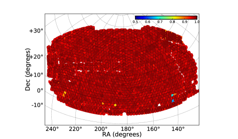
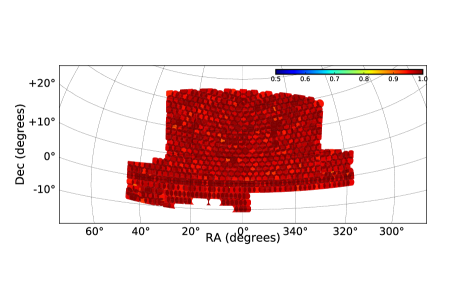
The creation of the large-scale structure catalogues from the BOSS spectroscopic observations is detailed in Reid et al. (2016). In brief, we consider the survey footprint, veto masks and survey-related systematics (such as fibre collisions and redshift failures) in order to construct data and random catalogues for the DR12 BOSS galaxies. The veto masks exclude 6.6% (9.3%) of the area within the north (south) galactic cap footprint, mostly due to regions of non-photometric quality but we also consider plate centerposts, collision priorities, bright stars, bright objects, Galactic extinction and seeing. The DR12 footprint is shown in Fig. 1 and Table 2 summarises our sample, which spans a completeness-weighted effective area of 9329 deg2 (after removing the vetoed area). The total un-vetoed area with completeness is 9486 deg2.
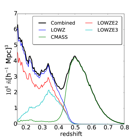
BOSS utilizes two target selection algorithms: LOWZ was designed to target luminous red galaxies up to , while CMASS was designed to target massive galaxies from . The spatial number density of these samples can be seen in Fig. 2. In previous papers, we analyzed these two samples separately, splitting at and omitting a small fraction of galaxies in the tails of both redshift distributions as well as the information from cross-correlations between the two samples. For the current analysis, we instead construct a combined sample that we describe in Section 2.3. With the combined map, we more optimally divide the observed volume into three partially overlapping redshift slices. As in Anderson et al. (2014b), the CMASS galaxies are weighted to correct for dependencies between target density and both stellar density and seeing. The definitions and motivations for these weights are described in Reid et al. (2016) and Ross et al. (2016). Clustering analyses of the DR12 LOWZ and CMASS samples, using two-point statistics, can be found in Cuesta et al. (2016a) and Gil-Marín et al. (2016a).
In addition to the LOWZ and CMASS samples, we use data from two early (i.e., while the final selection was being settled on) LOWZ selections, each of which are subsets of the final LOWZ selection. These are defined in Reid et al. (2016) and denoted ‘LOWZE2’ (total area of 144 deg2) and ‘LOWZE3’ (total area of 834 deg2). Together with the LOWZ sample, these three samples occupy the same footprint as the CMASS sample. As detailed in Ross et al. (2016), the ‘LOWZE3’ sample requires a weight to correct for a dependency with seeing. The LOWZ and LOWZE2 samples require no correction for systematic dependencies, as these were found to be negligible. We thus have four BOSS selections that we can use to construct a combined sample. This combined sample uses all of the CMASS, LOWZ, LOWZE2, and LOWZE3 galaxies with and allows us to define redshift slices of equal volume, thereby optimising our signal over the whole sample (see Section 2.3).
2.3 The Combined BOSS Sample
In this section, we motivate the methods we use to combine the four BOSS samples into one combined sample.
In principle, when combining galaxy populations with different clustering amplitudes, it would be optimal to apply a weight to each sample to account for these differences (Percival et al., 2004a). Ross et al. (2016) present measurements of the redshift-space correlation function for each of the four BOSS selections. Section 5.1 of that paper shows that the clustering amplitudes of each selection match to within 20 per cent and that combining the selections together where they overlap in redshift has no discernible systematic effect. Given the small difference in clustering amplitudes, a weighting scheme would improve the results by a negligible factor while imparting considerable additional complexity. We therefore choose to weight each sample equally when combining the catalogues. Each galaxy in this combined sample is then weighted by the redshift-dependent FKP weight (Feldman, Kaiser, & Peacock, 1994).
The clustering amplitude of different selections within the CMASS sample varies considerably more than the individual target selections (LOWZ/LOWZE2/LOWZE3/CMASS): the difference in clustering amplitude between the reddest and bluest galaxies within CMASS is a factor of two (Ross et al., 2014; Favole et al., 2015; Patej & Eisenstein, 2016). However, even when optimally weighting for this difference, the forecasted improvement in the statistical power of BOSS is 2.5 percent and our attempts to employ such a weighting in mock samples were unable to obtain even this improvement. Therefore, we have chosen to not introduce this additional complexity into our analysis.
We define the overall redshift range to consider for BOSS galaxies as . Below , the sample is affected by the bright limit of , and the BAO scale has been measured for galaxies in the SDSS-I/II main galaxy redshift survey (Strauss et al., 2002) by Ross et al. (2015). The upper limit of 0.75 is higher than in our previous analyses as we find no systematic concerns associated with using the data, but the number density has decreased to 10Mpc-3 at (a factor of 40 below its peak at ; see Fig. 2) and any additional data at higher redshift offer negligible improvement in the statistical power of the BOSS sample.
We defined the redshift bins used in this analysis based on an ensemble of 100 mock catalogues of the combined BOSS sample in the range . We tested several binning schemes by means of anisotropic BAO measurements on these mock catalogues. For each configuration, we ran an MCMC analysis using the mean value and errors from the BAO measurements, combining them with synthetic CMB measurements (distance priors) corresponding to the same cosmology of these mock catalogues. We chose the binning that provides the strongest constraints on the dark energy equation-of-state parameter . It consists of two independent redshift bins of nearly equal effective volume for and . In order to ensure we have counted every pair of BOSS galaxies, we also define an overlapping redshift bin of nearly the same volume as the other two, covering the redshift range . Using our mock catalogues, with the original LOWZ and CMASS redshift binning we obtain a 3.5% (9.6%) precision measurement of the transverse (line-of-sight) BAO scale in the LOWZ sample and a 1.8% (4.3%) precision measurement for the CMASS sample. With our chosen binning for the combined sample, we instead obtain transverse (line-of-sight) precision of 2.5% (6.3%) in our low redshift bin and 2.3% (5.6%) in our high redshift bin , comparable for the two samples by design. Our results in § 8.3 are consistent with these expected changes of precision relative to the LOWZ and CMASS samples. Measurements in the overlapping redshift bin are of course covariant with those in the two independent bins, and we take this covariance (estimated from mock catalogues) into account when deriving cosmological constraints. See Table 2 for a summary of the combined sample.
2.4 The NGC and SGC sub-samples
The DR12 combined sample is observed across the two Galactic hemispheres, referred to as the Northern and Southern galactic caps (NGC and SGC, respectively). As these two regions do not overlap, they are prone to slight offsets in their photometric calibration. As described in appendix A, we find good evidence that the NGC and SGC subsamples probe slightly different galaxy populations in the low-redshift part of the combined sample, and that this difference is consistent with an offset in photometric calibration between the NGC and the SGC (first reported by Schlafly & Finkbeiner 2011). Having established the reason for the observed difference in clustering amplitude, we decide not to re-target the SGC but rather to simply allow sufficient freedom when fitting models to the clustering statistics in each galactic cap, as to allow for this slight change in galaxy population. In particular, the different Fourier-space statistics are modelled with different nuisance parameters in the two hemispheres, as appropriate for each method. Using fits of the MD-Patchy mocks, we find that this approach brings no penalty in uncertainty of fitted parameters. We refer the reader to the individual companion papers for details on how this issue was tackled in each case.
3 Methodology
3.1 Clustering measurements
We study the clustering properties of the BOSS combined sample by means of anisotropic two-point statistics in configuration and Fourier space. Rather than studying the full two-dimensional correlation function and power spectrum, we use the information contained in their first few Legendre multipoles or in the clustering wedges statistic (Kazin et al., 2012).
In configuration space, the Legendre multipoles are given by
| (4) |
where is the two-dimensional correlation function, is the Legendre polynomial or order , and is the cosine of the angle between the separation vector and the line-of-sight direction. The power spectrum multipoles are defined in an analogous way in terms of the two-dimensional power spectrum
| (5) |
and are related to the configuration-space by
| (6) |
where is the spherical Bessel function of order . We use the information from the monopole, quadrupole and hexadecapole moments (, 2 and 4), which are a full description of the dependence of in the linear regime and in the distant observer approximation.
The configuration- and Fourier-space wedges, and correspond to the average of the two-dimensional correlation function and power spectrum over the interval , that is
| (7) |
and
| (8) |
Here we define three clustering wedges by splitting the range from 0 to 1 into three equal-width intervals. We denote these measurements by and .
The information content of the multipoles and the wedges is highly covariant, as they are related by
| (9) |
where is the average of the Legendre polynomial of order over the -range of the wedge,
| (10) |
More details on the estimation of these statistics using data from the BOSS combined sample can be found in the supporting papers listed in Table 1.
3.2 Parametrizing the Distance Scale
The BAO scale is measured anisotropically in redshift-space in both the two-point correlation function and the power spectrum. We measure the shift of the BAO peak position with respect to its position in a fiducial cosmology, which directly gives the Hubble expansion rate, , and the comoving angular diameter distance, , relative to the sound horizon at the drag epoch, (eq. 1). We define the dimensionless ratios
| (11) |
to describe shifts perpendicular and parallel to the line of sight. The anisotropy of galaxy clustering is also often parametrized using an isotropically-averaged shift and a warping factor with
| (12) |
Converting equation (12) to more physical quantities, we can define a spherically-averaged distance and an anisotropy parameter (often referred to as the Alcock-Paczynski parameter) as
| (13) |
| (14) |
Although these quantities are trivially interchangeable, we will adopt in each section the most natural parametrization. In particular, we quote our measurements in physical units: , , , and . We generally use and when referring to studies and checks on our mock catalogues and and when describing our systematic error budget. In our fiducial cosmological model, Mpc, and convenient approximations for the scaling of with cosmological parameters (including neutrino mass) can be found in Aubourg et al. (2015). Within CDM, the uncertainty in given Planck CMB constraints is 0.2%, substantially smaller than our statistical errors. However, changes to the pre-recombination energy density, such as additional relativistic species or early dark energy, can change by altering the age-redshift relation at early epochs.
4 Mock catalogues and the covariance matrix
We use mock galaxy catalogues to estimate the covariance matrix of our clustering measurements and to extensively test our methods. For this work, we utilized two distinct methods of mock galaxy creation: MultiDark-Patchy (hereafter MD-Patchy; Kitaura et al. 2016) and Quick Particle Mesh (QPM; White et al. 2014). MD-Patchy simulates the growth of density perturbations through a combination of second-order Lagrange perturbation theory and a stochastic halo biasing scheme calibrated on high-resolution N-body simulations. QPM uses low-resolution particle mesh simulations to evolve the density field, then selects particles from the density field such that they match the one- and two-point statistics of dark matter halos. Both mock algorithms then use halo occupation methods to construct galaxy density fields that match the observed redshift-space clustering of BOSS galaxies as a function of redshift. Each mock matches both the angular selection function of the survey, including fibre collisions, and the observed redshift distribution . A total of 1000 MD-Patchy mocks and 1000 QPM mocks were utilized in this analysis.
Analyses of previous data releases utilized mocks created from the PTHalos method (Manera et al., 2015). Comparison of the QPM and PTHalos in the context of our BAO analysis can be found in Vargas-Magaña et al. (2015), and a comparison of MD-Patchy to PTHalos, as well as other leading methods for generating mock catalogues, can be found in Chuang et al. (2015). Vargas-Magaña et al. (2016) directly compared the values and errors found in pre-reconstructed BAO analysis between PTHalos and QPM for the large-scale structure sample of the SDSS 11th data release (DR11). They found that the derived quantities, and , and their uncertainties, were consistent between the two methods.
Our reconstruction and BAO fitting procedures, as well as tests of the clustering measurements, have been applied to both sets (Vargas-Magaña et al., 2016; Ross et al., 2016). For details on the use of the mocks in the full shape analyses, see the respective papers (Table 1) for each individual analysis. Having two sets of mock simulations allows us to test the dependence of our errors on the mock-making technique. QPM and MD-Patchy differ in their methods of creating an evolved density field, as well as their underlying cosmology. As a conservative choice, our final error bars on all measurements, both BAO and RSD, are taken from the MD-Patchy covariance matrix because the errors obtained using the MD-Patchy covariance matrix are roughly per cent larger, and the clustering of the MD-Patchy mocks is a better match to the observed data. The larger derived error bar from the MD-Patchy covariance matrix is obtained both when fitting the observations and when fitting mock data.
For each clustering measurement, we use the distribution of the measured quantity measured from the mocks to estimate the covariance matrix used in all fittings. For the MD-Patchy mocks for the DR12 combined sample, distinct boxes were used for the NGC and SGC footprints, a change in practice compared to our analyses of previous data releases. Thus, the covariance matrices for the NGC and the SGC are each estimated from 997 total mocks222Three MD-Patchy mocks were removed from the final analysis due to unusual, non-Gaussian, clustering properties that were likely due to errors in the simulations.. The full procedure for estimating the covariance matrices is described in Percival et al. (2014), which includes the uncertainties in the covariance matrix when derived from a finite sample of simulations.
5 Post-reconstruction BAO measurements
5.1 Reconstruction

| Measurement | redshift | Beutler et al. (b) | Vargas-Magaña et al. | Ross et al. |
|---|---|---|---|---|
| [Mpc] | ||||
| [Mpc] | ||||
| [Mpc] | ||||
Following our previous work, we approximately reconstruct the linear density field in order to increase the significance and precision of our measurement of the BAO peak position. The reconstruction algorithm we use is described in Padmanabhan et al. (2012). This algorithm takes two input parameters: the growth rate parameter (eq. 3) to correct for redshift-space distortion effects and the galaxy bias parameter to convert between the galaxy density field and the matter density field. In the case of BOSS galaxies we find that the galaxy bias is a rather shallow function of redshift except for the very high redshift end, so a single value is assumed for the three redshift bins in our analysis. Furthermore, for a CDM cosmology the value of is not strongly redshift-dependent either, varying by 10 per cent in the range . Variations of this size in the input parameters have been proven not to affect in any significant way the post-reconstruction BAO measurements (Anderson et al., 2012). This allows us to run reconstruction on the full survey volume (as opposed to running the code on individual redshift bins) and thus take into account the contributions from larger scales to bulk flows. The values of the input parameters we used correspond to the value of the growth rate at for our fiducial cosmology, , and a galaxy bias of for the QPM and MD-Patchy mocks. For the data, we assumed a bias of . The finite-difference grid is (each cell being roughly 6Mpc on a side), and we use a Gaussian kernel of 15Mpc to smooth the density field, a choice found to provide conservative error bars in BAO fitting (Vargas-Magaña et al., 2015; Burden, Percival & Howlett, 2015).
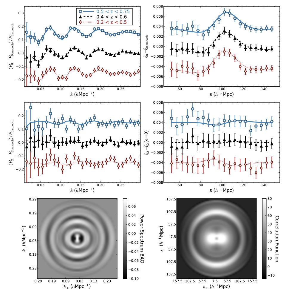
Fig. 3 displays the post-reconstruction BAO feature in the combined sample data. Each panel uses different means to isolate the BAO information. The upper panels represent the BAO information in the monopole of the clustering measurements; this information provides the spherically averaged BAO distance constraint. For the power spectrum, we display and for the correlation function , where the subscript ‘smooth’ denotes the best-fit model but substituting a template with no BAO feature for the nominal BAO template. One can observe that the spherically-averaged BAO feature is of nearly equal strength in each redshift bin, as expected given their similar effective volumes. Note that data points in are strongly correlated, while those in are more nearly independent. Qualitatively, our ability to measure the isotropic BAO scale comes down to our ability to centroid the BAO peaks in or to determine the phases of the oscillations in . Best-fit models are slightly offset horizontally because the best-fit values of are slightly different in the low, middle, and high-redshift bins. (Vertical offsets are added for visual clarity.)
The middle panels of Fig. 3 illustrate the information provided by the quadrupole of the clustering measurements, which constrains the anisotropy parameter (or, equivalently, ). The nature of the BAO signature is more subtle here, since if reconstruction perfectly removed redshift-space distortions and the fiducial cosmological were exactly correct then clustering would be isotropic and the quadrupole would vanish. For the power spectrum, we display and for the correlation function , where is computed using the same parameters as the best-fit model but with . For the redshift bin, is close to zero (the significance is 0.3 for both the power spectrum and the correlation function; see Table 3 in Beutler et al. 2016b), and thus no clear feature is observed in the data or the model. In the low and high redshift bins, is marginally significant ( for both) and of opposite signs. Thus, the data points and best-fit curves show weak features that are opposite in sign in the two redshift bins.
The bottom panel of Fig. 3 displays the BAO ring(s) in the redshift bin, as reconstructed from the monopole and quadrupole, thereby filtering the higher-order multipoles that are treated as noise in our analysis. The results are decomposed into the component of the separations transverse to and along the line of sight, based on , where represents either multiplied by the correlation function or for the power spectrum, represents either the separation, , or the Fourier mode, , is the 2nd order Legendre polynomial, , and . Plotted in this fashion, the radius at which the BAO feature(s) represents the spherically-averaged BAO measurement and the degree to which the ring(s) is(are) circular represents the AP test as applied to BAO measurements.
5.2 Measuring the BAO scale
Our companion papers Ross et al. (2016), Vargas-Magaña et al. (2016) and Beutler et al. (2016b) use the BAO signal in the post-reconstruction monopole and quadrupole, in configuration space and Fourier space, to constrain the geometric parameter combinations and . We now present a brief summary of these analyses and refer the reader to those papers for more details.
Ross et al. (2016) and Vargas-Magaña et al. (2016) measure the anisotropic redshift-space two-point correlation function. Both methods rely on templates for and , which have BAO features that are altered as function of the relative change in and away from the values assumed in the fiducial templates (which are constructed using the fiducial cosmology). These templates are allowed to vary in amplitude and are combined with third-order polynomials, for both and , that marginalize over any shape information. This methodology follows that of Xu et al. (2013); Anderson et al. (2014a) and Anderson et al. (2014b). Small differences between Ross et al. (2016) and Vargas-Magaña et al. (2016) exist in the modelling of the fiducial templates and the choices for associated nuisance parameters. The choices in Ross et al. (2016) are motivated by the discussion in Seo et al. (2015) and Ross et al. (2015), and they carry out detailed investigations to show that observational systematics have minimal impact on the BAO measurement. Vargas-Magaña et al. (2016) use as their fiducial methodology the templates and choices used in previous works (Cuesta et al., 2016a; Anderson et al., 2014a, b) enabling direct comparison of the results with those previous papers. In addition, Vargas-Magaña et al. (2016) perform a detailed investigation of possible sources of theoretical systematics in anisotropic BAO measurements in configuration space, examining the various steps of the analysis and studying the potential systematics associated with each step. This work extends the previous effort in Vargas-Magaña et al. (2014), which focused on systematic uncertainties associated with fitting methodology, to more general aspects such as the estimators, covariance matrices, and use of higher order multipoles in the analysis.
Beutler et al. (2016b) extract the BAO information from the power spectrum. The analysis uses power spectrum bins of and makes use of scales up to . The covariance matrix used in this analysis has been derived from the MD-Patchy mocks described in Section 4. The reduced for all redshift bins is close to 1.
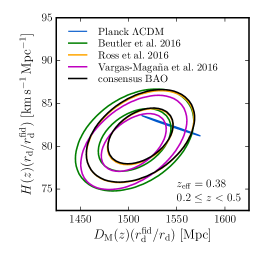
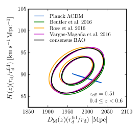
The two-dimensional 68 and 95 per cent confidence levels (CL) on and recovered from these fits are shown in Fig. 4, where we have scaled our measurements by the sound horizon scale in our fiducial cosmology, , to express them in the usual units of Mpc and . The corresponding one-dimensional constraints are summarised in Table LABEL:tab:combined_BAO. The results inferred from the three methods are in excellent agreement. As expected, given the small differences in methodology and data, the results of Ross et al. (2016) and Vargas-Magaña et al. (2016) are very similar. Tests on the results obtained from mock samples show that the results are correlated to a degree that combining them affords no improvement in the statistical uncertainty of the measurements. Differences between the results are at most 0.5 and are typically considerably smaller; these differences are consistent with expectations (further details of tests on mock samples are presented in Section 7.1). Thus, for simplicity, we select only the measurements and likelihoods presented in Ross et al. (2016) to combine with the power-spectrum BAO results and full-shape measurements. The consensus values are computed and discussed in Section 8.
6 Pre-reconstruction full-shape measurements
| Measurement | redshift | Satpathy et al. | Beutler et al. (b) | Grieb et al. | Sánchez et al. |
|---|---|---|---|---|---|
| multipoles | multipoles | wedges | wedges | ||
| [Mpc] | |||||
| [Mpc] | |||||
| [Mpc] | |||||


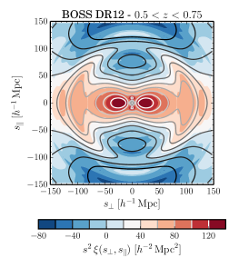
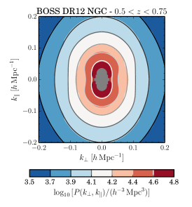
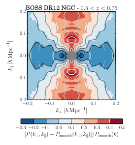
Fig. 5 shows the two-dimensional correlation function, (left panel), and power spectrum, (middle and right panels), of the NGC BOSS combined galaxy sample, in the redshift range . The figures for other redshifts and the SGC would look similar. The full shape of these measurements encodes additional information beyond that of the BAO feature. If we had access to the real-space positions of the galaxies and in the absence of AP distortions, the contours of these functions would correspond to perfect circles. However, the RSD caused by the peculiar velocities of the galaxies distort these contours, compressing (stretching) them along the line-of-sight direction in configuration (Fourier) space. These anisotropies encode information on the growth rate of cosmic structures, which can be used to constrain the parameter combination , where .
On large scales most of the information contained in and can be compressed into a small number of one-dimensional projections such as the their first few Legendre multipoles (e.g. Padmanabhan & White, 2008), or the clustering wedges statistic (Kazin et al., 2012). Each of the four supporting papers (Satpathy et al., 2016; Sánchez et al., 2016a; Beutler et al., 2016c; Grieb et al., 2016) uses the information of either multipoles or wedges in , in configuration or Fourier Space, employing different approaches to model the clustering statistics in the non-linear regime. The four methods were tested in high-fidelity mocks, via a blind challenge that we describe in Section 7.2 and that will later inform our systematic error budget. These measurements simultaneously capture the impact of the expansion rate, AP-effect and growth rate on the distribution of galaxies, allowing us to determine the parameter combinations , (or some combination thereof) and . Here we give a brief description of these analyses and refer the reader to those papers for more details on the measurements, modelling, fitting procedures and tests with mocks, as well as figures showing each of the measurements individually.
Satpathy et al. (2016) analyses the monopole and quadrupole of the two-point correlation function. The covariance matrix of these measurements is estimated using 997 MD-Patchy mock catalogues. The multipoles are modelled using Convolution Lagrangian Perturbation Theory (CLPT) and the Gaussian Streaming model (GSM) (Carlson et al., 2013; Wang et al., 2014). This model has been tested for both dark matter and biased tracers using N-body simulations (Wang et al., 2014) and has been tested for various observational and theoretical systematic errors (Alam et al., 2015b). Satpathy et al. (2016) fit scales between 25 and with bin width of and extract the cosmological and growth parameters with a Markov Chain Monte Carlo (MCMC) algorithm using CosmoMC (Lewis & Bridle, 2002).
Sánchez et al. (2016a) extract cosmological information from the full shape of three clustering wedges in configuration space, defined by dividing the range from 0 to 1 into three equal-width intervals, whose covariance matrix was obtained from a set of 2045 MD-Patchy mock catalogues. This analysis is based on a new description of the effects of the non-linear evolution of density fluctuations (gRPT, Blas et al. in prep.), bias and RSD that is applied to the BOSS measurements for scales between 20 and with a bin width of . Sánchez et al. (2016a) perform extensive tests of this model using the large-volume Minerva N-body simulations (Grieb et al., 2015) to show that it can extract cosmological information from three clustering wedges without introducing any significant systematic errors.
Beutler et al. (2016c) analyse the anisotropic power spectrum using the estimator suggested in Bianchi et al. (2015) and Scoccimarro (2015), which employs Fast Fourier Transforms to measure all relevant higher order multipoles. The analysis uses power spectrum bins of and makes use of scales up to for the monopole and quadrupole and for the hexadecapole. These measurements are then compared to a model based on renormalized perturbation theory (Taruya et al., 2010). This model has been extensively tested with N-body simulations in configuration space (e.g. de la Torre and Guzzo, 2012) and Fourier space (e.g. Beutler et al., 2012). The covariance matrix used in this analysis has been derived from Multidark-Patchy mock catalogues (The NGC uses only 2045 mock catalogues) and the reduced for all redshift bins is close to 1.
The methodology in Grieb et al. (2016) extends the application of the clustering wedges statistic to Fourier space. In order to make use of new estimators based on fast Fourier transforms (FFT; Bianchi et al., 2015; Scoccimarro, 2015), their analaysis uses the power spectrum clustering wedges, filtering out the information of Legendre multipoles . This information is combined to three power spectrum wedges, measured in wavenumber bins of , up to the mildly non-linear regime, . The full shape of these measurements is fitted with theoretical predictions based on the same underlying model of non-linearities, bias and RSD as in Sánchez et al. (2016a). Thus, these two complementary analyses represent the first time that the same model is applied in configuration and Fourier space fits. The methodology has been validated using the Minerva simulations and mock catalogues and found to give unbiased cosmological constraints. Besides the covariance matrix, which is derived from 2045 MD-Patchy mock catalogues, this analysis depends on a framework for the wedge window function, which was developed based on the recipe for the power spectrum multipoles of Beutler et al. (2014a). The power spectrum wedges of the NGC and SGC sub-samples in the low-redshift bin are modelled with two different bias, RSD, and shot noise parameters, while the intermediate and high redshift bins are fitted with the same nuisance parameters for the two sub-samples.
The constraints on , , and produced by each of the four individual methods are shown in Fig. 6 where, as before, we have rescaled our measurements by the sound horizon scale in our fiducial cosmology. The corresponding one-dimensional constraints are summarised in Table 4. The agreement between the results inferred from the different clustering statistics and analysis methodologies is good, and the scatter between methods is consistent with what we observe in mocks (see Section 7.2 and Fig. 10). In all cases the -wedges analyses give significantly tighter constraints than the multipole analyses, in both configuration space and Fourier space. The consensus constraints, described in §8.2 below, are slightly tighter than those of the individual wedge analyses. At all three redshifts and for all three quantities, mapping distance, expansion rate, and the growth of structure, the 68% confidence contour for the consensus results overlaps the 68% confidence contour derived from Planck 2015 data assuming a CDM cosmology. We illustrate the combination of these full shape results with the post-reconstruction BAO results in Fig. 11 below.
7 Systematic Error Estimation
7.1 Tests using MD-Patchy mock catalogues
Here we examine the consistency and correlation among the three methods applied to obtain post-reconstruction BAO measurements (described in Section 5) and the four methods applied to obtain pre-reconstruction full-shape constraints (described in Section 6). We do these comparisons using the results obtained from the fits to the MD-Patchy mock catalogues, which enabled at least 996 comparisons in all cases. These comparisons are used to inform the final systematic uncertainties, to be described in Section 7.4, that we apply to our measurements.
Table LABEL:tab:Pkxicompmocks compares the mean BAO results for the post-reconstruction correlation function and the power spectrum measurements and then the mean result when the individual results are combined as described in Section 8.1. The standard deviations are improved by the combination, as they are not perfectly correlated. The correlations between the correlation function and power spectrum results range between 0.88 and 0.90. The correlations between the two correlation function results are such that the optimal combination does not affect the standard deviation at the quoted precision. The results differ by an average of 0.002 for both and for , with the results having greater and lesser . These differences are smaller than the systematic modelling uncertainties will we adopt for each parameter (0.003 and 0.005), described in Section 7.4.
The detailed tests presented in Beutler et al. (2016b) and Vargas-Magaña et al. (2016) suggest no reason to believe any of the results should be biased relative to the others and they can be thus combined to produce the consensus results. The consensus results are obtained as described in Sánchez et al. (2016b). The results are slightly more precise and the consensus results are thus weighted towards these results. The consensus results are biased by at most 0.001 and the mean bias is 0.000. The consensus results are each biased by 0.002; this is 0.15 and is substantially smaller than the systematic uncertainty we adopt for .
Fig. 7 is an illustration of the results presented in Table LABEL:tab:Pkxicompmocks, with the and values converted to and values. Visually, it is clear that differences between the results using each methodology are negligibly small and that the consensus results match those expected for the MD-Patchy cosmology.
| sample | ||||
|---|---|---|---|---|
| : | ||||
| consensus | –0.001 | 0.012 | 0.002 | 0.014 |
| R | 0.000 | 0.013 | 0.001 | 0.015 |
| V | –0.001 | 0.014 | 0.001 | 0.016 |
| –0.001 | 0.013 | 0.003 | 0.015 | |
| : | ||||
| consensus | 0.001 | 0.011 | 0.002 | 0.013 |
| R | 0.001 | 0.012 | 0.001 | 0.014 |
| V | 0.000 | 0.012 | 0.002 | 0.013 |
| 0.000 | 0.012 | 0.002 | 0.014 | |
| : | ||||
| consensus | 0.000 | 0.011 | 0.002 | 0.013 |
| R | 0.002 | 0.012 | –0.001 | 0.015 |
| V | 0.000 | 0.012 | 0.001 | 0.014 |
| –0.001 | 0.012 | 0.001 | 0.015 |
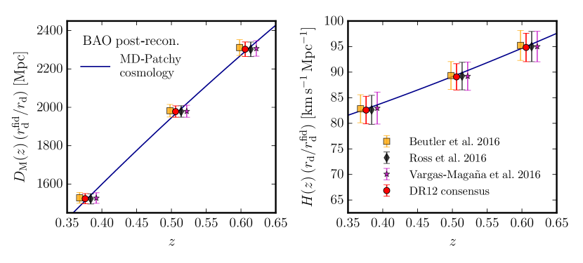
Table LABEL:tab:RSDcompmocks presents results for the four methods that apply pre-reconstruction full-shape fits to the DR12 BOSS galaxy data, including results for . Their combination, obtained as described in Section 8.1, produces the ‘combined’ results, and this combination reduces the standard deviations of the recovered results, taking advantage of partial complementarity (i.e., not complete correlations) among the methods. See Sánchez et al. (2016b) for further details.
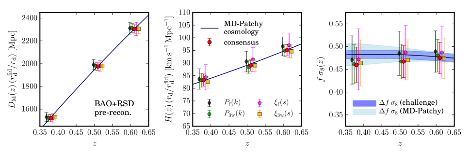
The biases in the combined and values from these pre-reconstruction analyses are below compared to the mock-to-mock dispersion, and they are smaller than the systematic uncertainty defined in §7.4. The biases on the recovered , 0.024, 0.016, and 0.003 in the three redshift bins, are up to compared to the mock-to-mock dispersion. Fig. 8 compares the results of our RSD fitting methods to the natural cosmology of the MD-Patchy mocks. When setting the systematic error for , we compare the bias inferred from the MD-Patchy mocks to the systematic error obtained using high resolution N-body simulations described in the next subsection. We use the maximum of these two numbers in each redshift bin as the systematic error.
| sample | ||||||
|---|---|---|---|---|---|---|
| : | ||||||
| consensus | –0.003 | 0.018 | 0.000 | 0.011 | –0.024 | 0.038 |
| 0.004 | 0.020 | 0.001 | 0.012 | –0.019 | 0.050 | |
| –0.001 | 0.021 | –0.004 | 0.020 | –0.012 | 0.053 | |
| –0.002 | 0.019 | 0.000 | 0.013 | –0.022 | 0.043 | |
| –0.008 | 0.020 | –0.004 | 0.025 | –0.011 | 0.067 | |
| : | ||||||
| consensus | 0.002 | 0.015 | 0.003 | 0.009 | –0.016 | 0.035 |
| 0.003 | 0.017 | 0.002 | 0.010 | –0.012 | 0.044 | |
| 0.001 | 0.019 | –0.005 | 0.018 | 0.002 | 0.049 | |
| 0.005 | 0.017 | 0.005 | 0.010 | –0.016 | 0.038 | |
| –0.006 | 0.017 | –0.007 | 0.022 | 0.004 | 0.060 | |
| : | ||||||
| consensus | 0.002 | 0.015 | 0.001 | 0.009 | –0.003 | 0.034 |
| 0.004 | 0.016 | 0.002 | 0.011 | –0.004 | 0.045 | |
| –0.001 | 0.017 | –0.005 | 0.017 | 0.011 | 0.045 | |
| 0.006 | 0.016 | 0.000 | 0.009 | 0.002 | 0.036 | |
| –0.005 | 0.016 | –0.006 | 0.022 | 0.009 | 0.058 |
7.2 RSD Tests using High Resolution Mocks
In addition to the large suite of covariance mocks, we also utilize a small series of high-fidelity mocks to test the accuracy and precision of our multiple RSD methods. Details of this “mock challenge” are presented in Tinker et al. (2016). There are two complementary sets of mocks. The first is a homogeneous set in which all mocks have the same underlying galaxy bias model built upon on the same cosmology, but each mock is an independent realization. These mocks have the same angular and radial selection function as the NGC DR12 CMASS sample. There are 84 mocks in total. The N-body simulations from which these cut-sky mocks were created use the high-resolution code GADGET2 (Springel, 2005), using input parameters to ensure sufficient mass and spatial resolution to resolve the halos that BOSS galaxies occupy. The second is a heterogeneous set in which different galaxy bias models are built upon the same simulation. Thus these mocks have not just the same underlying cosmology, but also the same large scale structure. But the galaxy bias varies at the per cent level. These mocks are built on periodic cubes of per side—roughly 4 times the volume of the DR12 CMASS sample. We use three different bias models in the second set of simulations. The second set of mocks are based on the Big MultiDark simulation (Riebe et al. 2013).
The first set of high resolution mocks tests quantifies the accuracy of the methods, including all aspects of the cut-sky analysis, while the second tests for possible theoretical systematics associated with the complexities of galaxy bias. Although the second set of mocks does not span the full possible range of galaxy bias models, they provide confidence that the methods are accurately recovering for the conventional space of cosmologies and galaxy evolution models. We use the quadrature sum of the errors on from these two sets of mocks as an estimate of the systematic error from the high-resolution mocks. As we will show, in some cases the error from the high-resolution mocks is smaller than the error obtained from the MD-Patchy mocks described in the previous section (the ‘’ column in Table LABEL:tab:RSDcompmocks). To be conservative, we adopt the larger of the errors obtained from the high resolution mocks and the MD-Patchy mocks as our final systematic error for a given redshift bin.
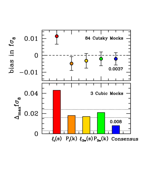
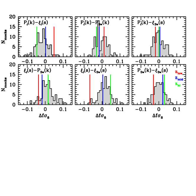
Each of the four RSD methods used in our consensus results were applied to 84 cut-sky mocks. Figure 10 shows how the differences among all four methods in the values derived from the DR12 data compare to the expectations from the cut-sky mocks. Each panel shows between two methods for each redshift bin, and the distribution of from the 84 mocks. The differences between the four methods applied to BOSS data, listed in Table 4, are in line with expectations from the differences between methods applied to the same mock survey.
The top panel in Figure 9 shows the bias in each full shape method when applied to the cut-sky mocks. The error bars represent the standard error in the mean. For each cut-sky mock, the results of the four RSD methods were combined in the same manner as our consensus results. Averaging over all 84 mocks, we find only a modest mean bias in the measured value of of 0.0018. This value is smaller than the statistical precision of the mean derived from 84 mocks, which is 0.0037, and so is not statistically significant. We adopt 0.0037 as an estimate of the potential bias of based on these mocks. To quantify a systematic variance in our RSD methods, we also applied the same analysis to the three cubic mocks with different bias models. Because these mocks are built on the same N-body simulation, there is little statistical significance in the comparison between the derived and the expected value. However, given that the mocks are built on the same large scale structure, any differences in the derived values from mock-to-mock represent systematic variations in the accuracy of the methods under different galaxy bias models. Thus, we use the maximal difference in between the three mocks as our systematic error from this test. The bottom panel of Figure 9 shows the quantity for all four full-shape methods as well as the consensus value. For the consensus value, we find the range in values to be 0.008. We then place a total systematic error on from the high-resolution mocks by adding 0.0037 and 0.008 in quadrature, yielding a value of 0.009 rms; however, we note that more exotic galaxy formation models might produce larger effects.
In principle, we can use these same high resolution mocks to quantify a systematic error on from the full shape analyses. Using the same procedure described above, where the cut-sky mocks define a bias and the cubic mocks estimate a systematic variance, we find a total error in of 0.0021. We will discuss this further in the following subsection.
The bottom panel of Figure 9 also shows the bias in the consensus values with respect to the MD-Patchy mocks. These bias values are shown with the horizontal dotted lines. From top to bottom, respectively, they represent the low redshift bin, the middle redshift bin, and the high redshift bin. The error from the MD-Patchy mocks is larger than that derived from the high-resolution mocks for the low and middle redshift bins (see the exact values in Table LABEL:tab:RSDcompmocks). Thus, for the systematic error in , we use the values from the MD-Patchy mocks for those two redshift bins, and we use the value from the high resolution mocks for the high redshift bin.
7.3 Tests of BAO Fitting Methodologies
Anderson et al. (2014b) provides an extensive discussion of systematic errors for the BAO measurements from the reconstructed density field. The adopted estimate was 0.003 in for systematics in the clustering measurements and fitting systematics, 0.003 in for astrophysical systematics involving galaxy bias, and 0.005 in for additional clustering and fitting systematics, all taken in quadrature. Anderson et al. (2014b) does not identify any dominant systematic of this type, arguing that all known effects were plausibly below 0.001. The clustering and fitting systematics in the monopole include effects such as mismatching of the power spectrum template and averaging across a finite redshift range. The clustering and fitting systematics in the quadrupole were additionally due to uncertainties in the redshift distortion modelling, possible small effects due to averaging over the finite redshift range, and a persistent small bias in the estimation of in our mock catalogues. The astrophysical systematics were due to potentially uncorrected shifts due to galaxy bias, despite past experience that reconstruction tends to null these shifts.
For the present work, we believe that several aspects of the results have improved. We have used several different fitting codes among the various methods and found good performance with all. Thepsuriya & Lewis (2015) further limits the template errors, in particularly finding only small shifts with changes in the extra relativistic species , a parameter that in any case has been more sharply limited by recent Planck results (Planck Collaboration XIII, 2015). Most notably, the measurement of is less biased than before, giving us substantially more confidence in the anisotropic measurement.
Vargas-Magaña et al. (2016) provides an additional exploration of potential sources of theoretical systematic uncertainty in the anisotropic BAO analysis of the completed BOSS galaxy samples. This paper also incorporates results from previous systematic error analyses (Vargas-Magaña et al., 2014; Cuesta et al., 2016a; Vargas-Magaña et al., 2015; Ross et al., 2016; Beutler et al., 2016b) to obtain a fuller accounting of potential systematic uncertainties. Vargas-Magaña et al. (2016) explores the anisotropic BAO methodology in a step-by-step manner, studying concerns such as (but not limited to): the effect of using different 2-point estimators in configuration space; the effect of using a finite sample of random catalogues; the manner in which the covariance matrix is produced; and the fiducial cosmology assumed in the analysis. Most variations were found to be very small, below 0.0005. The more important terms are variations induced by changes in reconstruction smoothing length, by changes in covariance matrix estimation, and by variations in the fiducial cosmology for the distance-redshift relation. However, these are all modest in size, around 0.001.
Adding the various terms in quadrature, Vargas-Magaña et al. (2016) estimates the systematic errors due to analysis and fitting procedures to be 0.002 for and 0.003 for .
7.4 Summary Model of Systematic Errors
Having discussed these tests of our methodologies, we now bring the results together to estimate a systematic error budget for the consensus results. We note that while we have tested a wide range of variations in our analysis procedures, as well as several sets of mock catalogues, this necessarily depends on some extrapolation to the unknown. As such, we opt to round up to an estimate of 0.003 in and 0.005 in for systematics in the clustering measurements and fitting methodologies. This is the same as the estimate in Anderson et al. (2014b). We treat these two errors as uncorrelated.
As stated in the previous subsection, we believe that the systematic control on BAO fitting has continued to improve relative to Anderson et al. (2014b). However, these improvements in the BAO analysis must be balanced against the fact that the reconstructed results are now being combined with fits to the full anisotropic clustering of the unreconstructed density field. In particular, while much of the information comes from the BAO, some results from the Alcock-Paczynski signal from the broadband clustering, which is partially degenerate with the RSD anisotropies. Therefore, errors in the RSD modelling could create systematic biases in . We therefore opt to keep the error at 0.005, even though the BAO fitting studies themselves do not indicate this much uncertainty.
We also continue to estimate an additional systematic error on of 0.003, to be added in quadrature so as to yield a total of 0.0042, resulting from astrophysical systematics involving galaxy bias, following Anderson et al. (2014b). We note that our fits to mock catalogues continue to return smaller shifts than this, despite variations in the physical models. However, more extensive work with N-body simulations and more complicated halo occupation models is needed to confidently shrink this error term.
As in Anderson et al. (2014b), we explicitly exclude from the systematic error budget the possible shift in the acoustic peak due to a coupling of the low-redshift galaxy density field to the small relative velocity between baryons and cold dark matter at high redshift (Tseliakhovich & Hirata, 2010; Dalal et al., 2010; Yoo et al., 2011; Slepian & Eisenstein, 2015; Blazek et al., 2016; Schmidt, 2016). Whether this effect exists at a measurable level remains speculative, but observational work from BOSS argues that it is subdominant as a systematic error. Yoo & Seljak (2013) first investigated relative velocities in the power spectrum of BOSS DR9 galaxies, placing an upper limit on their impact. Beutler et al. (2016a) sought the effect in the cross-correlation of the WiggleZ and BOSS survey, again finding no detection. More recently, Slepian et al. (2016b) search for the distinctive acoustic-scale signature of this coupling in the three-point correlation function of DR12 CMASS galaxies. They find no detection and use the results of Blazek et al. (2016) to place an 0.3% rms limit on the bias on the BAO-inferred distance scale resulting from the relative velocities. We have also tested whether including these velocities in the BAO template, following Blazek et al. (2016) and marginalizing over a free amplitude, alters the best fit to our pre-reconstruction measurements. We find at most a 0.3 shift in , consistent with the results of Slepian et al. (2016b), indicating no preference for relative velocities in the two-point clustering. Schmidt (2016) argues for further acoustic-scale imprints of the relative variations of the baryon and dark matter density fields, highlighting the possibility that galaxy bias could depend on the small large-scale variations in the baryon fraction (Barkana & Loeb, 2011). This remains an open topic — see Soumagnac et al. (2016) for a novel but inconclusive search for a related effect.
Turning now to the RSD fits, Fig. 8 compares the two values for the systematic error on from the MD-Patchy mock comparison and the high-resolution challenge mocks described in sections 7.1 and 7.2. The MD-Patchy bias is larger for the low- and intermediate-redshift bins, while the error from the high resolution mocks is larger for the high redshift bin. We follow a conservative approach and define the systematic errors for each redshift bin as the maximum of these two estimates. We therefore adopt systematic errors on given by 0.024, 0.015 and 0.009 for our low, intermediate and high redshift bins, respectively. We note that the middle bin differs (negligibly) from the 0.016 in Section 7.2 due to slight evolution late in the development of the paper.
In principle, this systematic error in would be correlated with the systematic error in . However, the correlations in the statistical errors of these parameters are not particularly large ( for all redshift bins) due to the sizeable role of the BAO, which is less degenerate with modulations of the quadrupole amplitude caused by the RSD. Taking the slope of the statistical error correlation as an indication of the coupling in the quadrupole between the broadband Alcock-Paczynski effect and the RSD, our systematic errors on would map to errors on of 0.0033, 0.0018, and 0.0012 for each of the redshift bins. These are smaller than the 0.005 rms error from Anderson et al. (2014b), as is the error estimated directly from the high resolution mocks in section 7.2, 0.0021. Coupled with the improved fitting of , we opt to keep the systematic error on at 0.005 rms. We neglect the correlations of this with the systematic error for simplicity and assume the same systematic errors in and for out BAO-only, full-shape and final BAO+FS constraints.
Having specified our estimate of independent systematic uncertainty in , , and , we also need to specify how these might correlate between our three redshift bins. Declaring the systematic errors to be independent between the redshift bins would be over-optimistic as regards redshift-independent shifts if in fact the errors in the three bins are highly correlated. We do expect substantial correlations across redshift: our fitting methodologies are the same at each redshift, and the galaxies in the three samples are rather similar, all red galaxies with rather little change in luminosity or clustering amplitude. We see little reason, for example, that astrophysical shifts of the acoustic scale due to galaxy bias would differ much between LRGs and those at . On the other hand, treating the errors as fully correlated is also an extreme, as it excludes mild systematic variation in redshift. We therefore adopt an intermediate ansatz by introducing off-diagonal redshift couplings of 0.75 in the reduced covariance matrix representing our systematic errors on all parameters. This corresponds to superposing a fully correlated error that is 0.87 of the total with additional independent errors per redshift bin that are 0.50 of the total. Alternatively stated, in this ansatz, the variance of the common mode is 10-fold larger than the variance of the two other modes.
We note, however, that because the systematic error for changes with redshift (unlike for and ), the common mode favoured by this ansatz is not redshift independent. A redshift-independent shift in is constrained to have 0.008 rms in our model. For comparison, had we chosen the three bins to be fully independent, the constraints on the redshift-independent shift would have been 6% stronger. A correlation coefficient around 0.45 maximizes the error for this shift, but at a level only 12% worse than our model. Noting that the systematic errors are subdominant to statistical errors in all cases, we conclude that the choice of correlation coefficients for , , or does not substantially impact our cosmological conclusions.
8 Results from the BOSS combined sample
8.1 Combining measurements and likelihoods
| Measurement | redshift | BAO-only | Full-shape | BAO+FS |
|---|---|---|---|---|
| [Mpc] | ||||
| [Mpc] | ||||
| [Mpc] | ||||
| - | ||||
| - | ||||
| - |
| Mean | (lower) or (upper) | |||||||||||
| 1518 | 22 | 10000 | -750 | -3675 | -4686 | 239 | 1781 | 495 | -166 | -85 | 18 | |
| 81.5 | 1.9 | 2280 | 10000 | -2904 | 126 | -4426 | 1196 | -380 | 465 | -73 | 1.6 | |
| 0.497 | 0.045 | 3882 | 3249 | 10000 | 1764 | 1588 | -4669 | 299 | -79 | 625 | 0.034 | |
| 1977 | 27 | 4970 | 1536 | 1639 | 10000 | -737 | -3662 | -4764 | 375 | 1922 | 18 | |
| 90.4 | 1.9 | 1117 | 4873 | 1060 | 2326 | 10000 | -2855 | 253 | -5140 | 1452 | 1.4 | |
| 0.458 | 0.038 | 1797 | 1726 | 4773 | 3891 | 3039 | 10000 | 1733 | 1631 | -4990 | 0.025 | |
| 2283 | 32 | 1991 | 984 | 237 | 5120 | 1571 | 2046 | 10000 | -906 | -4042 | 24 | |
| 97.3 | 2.1 | 520 | 2307 | 108 | 1211 | 5449 | 1231 | 2408 | 10000 | -2565 | 1.7 | |
| 0.436 | 0.034 | 567 | 725 | 1704 | 1992 | 1584 | 5103 | 4358 | 2971 | 10000 | 0.026 | |


As described in the previous sections, we have computed the parameter combinations , and in three overlapping redshift slices using multiple clustering statistics and modelling assumptions. Although they are of course covariant, these estimates do not contain the same information nor are they affected by noise in the same way. This implies that their combination can have a higher constraining power than each individual measurement. With this in mind, we combine the posterior distributions obtained from our BAO-only and full-shape measurements into sets of consensus constraints that optimally capture all of the information they provide. To do this we follow the method of Sánchez et al. (2016b), which we summarize below.
We wish to combine the results of different statistical analyses applied to a given data set, each leading to an estimate of the same set of parameters. If the posteriors of these parameters are well described by a multivariate Gaussian distribution, the results of any given method can be represented by an array of measurements and their corresponding covariance matrix . The full set of measurements obtained from the different methods corresponds to a set of highly correlated measurements. As shown in Sánchez et al. (2016b), it is possible to compress the full information contained in these measurements into a single set of consensus values, , with its corresponding covariance matrix, . A crucial ingredient for this combination is the total covariance matrix
| (15) |
where each off-diagonal block represents the cross-covariance matrix between the results of methods and . In order to write down the explicit solutions for and we first define a total precision matrix as
| (16) |
which we divide in blocks of size as
| (17) |
The general expression for can then be written as
| (18) |
while is given by
| (19) |
This methodology can also be used to combine posterior distributions with different number of parameters. In this case the final consensus constraints will correspond to the parameter space defined by the union of those of the individual measurements. In particular, in order to combine our BAO-only and full-shape constraints we are interested in the case in which a given method gives constraints on the first parameters only, with an associated covariance matrix . These results can be considered as including a constraint on the remaining parameter, but with an infinite uncertainty, that is
| (20) |
In the total covariance matrix the rows and columns corresponding to the undetermined parameter will be zero. This structure will be inherited by , where also the diagonal entry corresponding to this parameter will cancel. It is then possible to apply equations (18) and (19) to derive the final consensus values that combine the information from all measurements.
Sánchez et al. (2016b) tested this technique by using it to combine the results obtained from the application of the BAO-only and full-shape analyses described in Sections 5 and 6 to a sub-set of 999 MD-Patchy mock catalogues described in Section 4, showing that in all cases the obtained consensus constraints represent a reduction of the allowed region of the parameter space with respect to the results of each individual method.
8.2 Consensus constraints from BOSS
As shown in our companion papers, the posterior distributions recovered from the different analysis methodologies applied to BOSS are well described by Gaussian multivariate distributions, which means that we can apply the methodology described in the previous section to obtain our consensus results. We will obtain three sets of consensus results, from the following measurements: post-reconstruction BAO (denoted as BAO-only), pre-reconstruction full-shape measurements (denoted as full-shape or FS), and finally, a final consensus set from combining post-reconstruction BAO with pre-reconstruction full-shape measurements, denoted as BAO+FS. For BAO-only measurements, which are only sensitive to the geometric quantities and , we have , while for full-shape fits, which can also constrain , .
The application of equations (18) and (19) requires the knowledge of the total covariance matrices for each case. For the diagonal blocks , we use the covariance matrices derived from the posterior distributions of each analysis method. We construct the off-diagonal blocks using the cross-correlation coefficients derived by Sánchez et al. (2016b) from the application of the different methods to the MD-Patchy mock catalogues.
The solid black contours in Figures 4 and 6 correspond to the BAO-only and full-shape consensus constraints, respectively, derived by applying equations (18) and (19) to the results of our companion papers. The final covariance matrices of our consensus constraints are obtained by adding the matrices derived from the combination of the posterior distributions, which represent the statistical uncertainties of our results, with that of the systematic errors described in Section 7.4. The corresponding one-dimensional marginalized constraints are listed in the third and fourth columns of Table 7, where the first error accompanying each value correspond to the statistical 68 per cent CL, and the second one represents the systematic error assigned to these results (see Section 7.4).
Fig. 11 illustrates the principal observational results of this paper in the form of confidence contours from the BAO-only (black) and full-shape (green) consensus constraints in each of our three redshift bins, for different pairwise combinations of , , , , and the Alcock-Paczynski parameter . The filled contours represent the combination of these results into the final set of BAO+FS consensus constraints representing the full information obtained from our pre- and post-reconstruction clustering measurements. The corresponding one-dimensional constraints are quoted in the last column of Table 7 and shown as a function of redshift alongside the CDM best-fit Planck prediction in Fig. 12. The covariance and precision matrices are in Table 8.
The statistical uncertainties in , , and are all reduced in our final consensus values, with respect to those in any individual method or in the BAO-only and full-shape consensus constraints. The improvement in the statistical uncertainty, with respect to the smallest quoted uncertainty in each of the individual measurements, is typically 15% for , 20% for , and 10% for . These improvements are in agreement with what is expected from tests on the mocks (Sánchez et al., 2016b). Figure 9 further shows that, on high-fidelity mocks, consensus results show a smaller systematic bias than each individual method. It is this final set of consensus values and derived likelihoods that we use in our cosmological analysis in Section 9.
When expressed in terms of the average distance , our final BAO+FS consensus constraints correspond to
| (21) | ||||
| (22) | ||||
| (23) |
These values correspond to distance measurements of 1.1% precision for our low-redshift bin and 1.0% for the intermediate and high-redshift bins. The 0.2% statistical error on , based on Planck 2015 CMB constraints assuming standard matter and radiation content, makes a negligible contribution when added in quadrature. These values are covariant, though the first and third are only weakly so; one should use the full likelihood for fitting models.
Although it is not appropriate for cosmological fits, it can be useful as a metric to compute the aggregate precision of the measurement by combining across the three redshift bins, including our systematic error estimates. Doing this, we find a precision of 1.0% on the transverse distance scale, 1.6% on the radial distance scale, and 0.8% on the spherically averaged . We also find a 5.7% aggregate precision on . In all cases, these were computed as the error on a single rescaling of the best-fit measurements in the three redshift bins for the chosen parameter, holding the other six measurements fixed. In the case of , we held fixed. If instead one marginalizes over the other six dimensions, the aggregate errors degrade slightly by a factor of 1.1–1.2. We note that the performance on specific parametrized models, such as in Section 9, can be different than these values, as they correspond to other weightings of the various measurements.
In Table 7, the 1-dimensional errors on and from the full-shape analyses are only slightly worse than those of the BAO-only analyses even though the constraints on these quantities come mainly from BAO and the BAO-only analyses take advantage of precision gains from reconstruction. Figure 11 helps to resolve this conundrum. The values of and are more strongly correlated for the BAO-only analysis, so while the constraints from post-reconstruction BAO-only are appreciably tighter than those from pre-reconstruction full-shape, the marginalized constraints on and are not. The constraints on from sub-BAO scales in the full-shape analyses help to break the degeneracy between and , leading to rounder confidence contours and smaller errors on . The combined BAO+FS contours are able to take advantage of both the sharpening of the BAO feature by reconstruction and the improved degeneracy breaking from the sub-BAO Alcock-Paczynksi effect. In all of the projections shown here, the 68% CL contour from our consensus constraints overlaps the 68% CL contour from the Planck 2015 CMB results assuming a CDM cosmological model, demonstrating impressive success of this model in reproducing the expansion history and rate of structure growth over the redshift range . We provide more detailed assessment of the cosmological implications of these measurements in §9.
8.3 Comparison to Past Work
| [Mpc] | [Mpc] | [Mpc] | [Mpc] | ||||
| DR9 | Anderson et al. (2012, 2014a) | — | — | — | |||
| DR10 | Anderson et al. (2014b) | — | — | ||||
| Tojeiro et al. (2014) | |||||||
| DR11 | Anderson et al. (2014b) | — | — | ||||
| DR12 | Chuang et al. 2016 | ||||||
| Cuesta et al. 2016a | |||||||
| Gil-Marín et al. 2016a | |||||||
| Gil-Marín et al. 2016b | — | — | |||||
| Gil-Marín et al. 2016c | — | — | |||||
| Pellejero-Ibañez et al. 2016 | — | — | |||||
| Slepian et al. 2016a | — | — | — | — | — | ||
| Wang et al. 2016 | — | — | |||||
| Zhao et al. 2016 | — | — | |||||
| Cuesta + G-M 2016 a | |||||||
| G-M et al. 2016 (a+b+c) | — | — | |||||
| Final | This work |
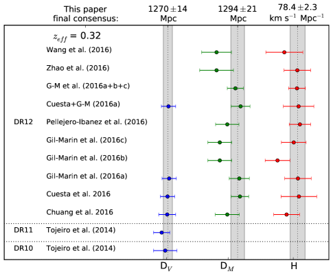
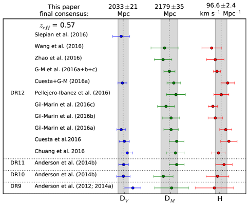
In this section, we compare our results to previous work. We begin by summarizing BAO-distance measurements made by the BOSS team since DR9, which we collect in Table 9 and Fig. 13. We quote values at and , corresponding to the effective redshifts of the LOWZ and CMASS samples. To put the results of this paper in the same context, we extrapolate our distance measurements to the above values of effective redshift, assuming a flat CDM cosmology (). The DR9, DR10, and DR11 measurements use 2-point statistics in configuration and Fourier space, and the improvement of precision with the growing BOSS footprint is evident in the statistical error bars, while the agreement between the measurements is reassuring. The DR12 measurements come from a variety of methods including 3-point statistics in both configuration and Fourier space as well as different approaches to redshift binning and quantifying anisotropy to separate and . Some of these analyses use full-shape information and others use BAO only. Most of the DR12 analyses listed in Table 9 use the LOWZ and CMASS catalogues, while this paper and its supporting papers use a combined sample that is optimized to have better statistical power. The Zhao et al. (2016) and Wang et al. (2016) results listed in Table 9 also use the combined sample.
We briefly review the different approaches of the previous DR12 papers. Because the underlying galaxy data are the same, we expect consistency at the 1 level or better, but the robustness of distance-scale inferences across such a wide range of analysis methods is reassuring nonetheless. Chuang et al. (2016) use 2-point functions in configuration space and seek to achieve the best systematic free measurement of distances and growth rate measurements by marginalizing over several nuisance terms in their analysis. Cuesta et al. (2016a) follows exactly the same methodology as in our DR10 and DR11 analysis (Anderson et al., 2014b) with the same type of catalogues (LOWZ and CMASS). We expect the increase of statistical power of the derived parameters from Anderson et al. (2014b) to Cuesta et al. (2016a) to be purely due to the increase in our survey volume. Gil-Marín et al. (2016a) and Gil-Marín et al. (2016b) used line of sight power-spectrum to measure the BAO position and growth rate respectively. Slepian et al. (2016a) uses the 3-point function in configuration space to measure the BAO position. Gil-Marín et al. (2016c) uses full-shape measurement of the 3-point statistics and 2-point statistics in Fourier space to constrain the BAO and RSD parameters. Our analysis presented in this paper does not involve using any 3-point function statistics. In principle, there is additional information that can come from the higher order correlation function (see discussions of information correlation between 2- and 3-point functions in Slepian et al. (2016a) and Gil-Marín et al. (2016c)). Wang et al. (2016) and Zhao et al. (2016) analyzed the BAO distances in nine redshift bins instead of the three in our analysis in both configuration space and Fourier space. Pellejero-Ibañez et al. (2016) analyzed the sample with minimal assumptions of cosmological priors and found consistent results as our analysis.
A comparison with Cuesta et al. (2016a) and Gil-Marín et al. (2016a) is of particular interest, as those papers present similar configuration and Fourier space analyses to the ones used here, for the same BOSS data set, but breaking the samples by the LOWZ and CMASS target selections rather than the finer redshift binning adopted in this paper. In the following discussion we will focus on their consensus results, obtained from combining the likelihoods derived from the correlation and power spectrum. Those consensus results are presented in Gil-Marín et al. (2016a). The performance of our updated methodology can be tested against the above consensus results by comparing the precision in cosmic distance measurements. We make an approximate comparison by equating LOWZ to our low redshift bin, and CMASS to our high redshift bin. Note that our low redshift bin has a larger effective volume than the LOWZ sample , and our high redshift bin has a smaller effective volume than the CMASS sample, . There is a trade-off in the precision of the low redshift bin, at the expense of having less precision in the high redshift bin, motivated by the redshift boundary being shifted from to . To clarify the comparison, we will rescale in the following discussion the LOWZ uncertainties by a factor of and the CMASS uncertainties by a factor of , so the reader should assume this factor implicitly in all text throughout this section. However, Fig. 13 and Table 9 have no such corrections applied to them.
For comparison, we focus on the constraints, as these provide the most information from the post-reconstruction BAO analysis and we regard the LOWZ volume as too small to obtain robust likelihoods (the LOWZ likelihood is what was used in the Cuesta et al. 2016a cosmological analysis). The consensus precision on from the combination of the Cuesta et al. (2016a) and Gil-Marín et al. (2016a) results is 1.3 per cent for LOWZ and 1.0 per cent for CMASS, after the above scaling by . The consensus precision we obtain (see Section 8.2) is 20 per cent better at low redshift and the same at high redshift, and these constraints come almost entirely from the post-reconstruction BAO analysis (see the second column of Fig. 11). Our improvement at low redshift is compatible with the fact that our error in is smaller than the standard deviation of the mock samples (see Table 5) by 20 per cent, while the results presented in Cuesta et al. (2016a) obtained slightly worse precision than the equivalent quantity from the mocks. Such fluctuations in precision are consistent with those found in our mock samples. In terms of the standard deviation, the consensus mock results for in Cuesta et al. (2016a) agree with the consensus results presented in Table LABEL:tab:Pkxicompmocks, at the number of significant digits we quote. Thus, results from this comparison are consistent with the expectation from the tests in mock catalogues described in Section 2.3.
Figure 14 plots our BAO-only results in the wider context of other surveys and higher redshift measurements from the BOSS Ly forest. Blue, green, and red curves/points show , , and , divided by and with redshift scalings that fit all three curves on the same plot with visible error bars. The three lines show the predictions of a CDM model with the Planck 2015 parameters. Symbols show BAO measurements from to collected from 6dFGS (Beutler et al., 2011), SDSS-I/II (Percival et al., 2010; Ross et al., 2015), WiggleZ (Blake et al., 2011a, b), and the BOSS Ly forest auto- and cross-correlations (Delubac et al. 2015 and Font-Ribera et al. 2014, respectively), in addition to the BOSS galaxy measurements described here. The Percival et al. (2010) analysis includes SDSS LRGs and overlaps significantly with BOSS, while the main galaxy sample (MGS) analyzed, with reconstruction, by Ross et al. (2015) is essentially independent. The WiggleZ survey volume also overlaps BOSS, but 6dFGS is again independent. We find consistency across all galaxy BAO measurements. Moderate tension with the Ly forest BAO measurements remains, as discussed in detail by Delubac et al. (2015) and Aubourg et al. (2015). BAO analyses of the DR12 Ly forest data set are in process (J. Bautista et al., in prep.).
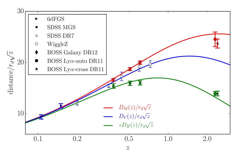
Next we compare our results to those from the literature. As before, we begin by collecting the work done by the BOSS team, which we summarize on the left-hand side of Fig. 15. We include measurements and quoted uncertainties from DR11 studies (Alam et al., 2015b; Beutler et al., 2014a; Samushia et al., 2014; Sánchez et al., 2014) and DR12 (Gil-Marín et al., 2016b; Chuang et al., 2016). The improved precision at low redshift in the present analysis greatly helps to test the predictions of structure growth in the universe, showing consistency with CDM and GR. We find excellent consistency among different methods and data releases. Given the small area increase between DR11 and DR12, the differences seen in Figure 15 are likely a consequence of different redshift binning and analysis/modelling methods. A more detailed study of the impact of different methodologies on measurements, using high-fidelity mocks, can be found in Tinker et al. (2016) for DR12 measurements.
The right panel of Figure 15 compares our measurements of results those from other surveys: 2dfGRS (Percival et al., 2004b), 6dFGS (Beutler et al., 2012), GAMA (Blake et al., 2013), WiggleZ (Blake et al., 2012), VVDS (Guzzo et al., 2008), and VIPERS (de la Torre et al., 2013), as well as the measurements from the SDSS-I and -II main galaxy sample (Howlett et al., 2015, MGS) and the SDSS-II LRG sample (Oka et al., 2014, DR7). The measurements plotted are conditional constraints on based on the Planck 2015 CDM cosmological model. This can be seen as a direct test of General Relativity. We find that our results confirm the validity of General Relativity. We also find reassuring consistency between our measurements and those by different surveys.
It is also interesting to compare this paper’s full-shape results (Table 7) with the full-shape analysis of the DR12 LOWZ and CMASS samples, done in Fourier space by Gil-Marín et al. (2016b) (scaled again by factors). Approximating LOWZ to our low redshift bin and CMASS to our high redshift bin, we find a measurement of 1.7% in the low redshift bin and 1.8% in the high redshift bin, which compares to 2.3% and 1.8% in Gil-Marín et al. (2016b), respectively. Regarding , our measurement of 2.8% in both the low and high redshift bins compares to 3.8% and 3.6% in Gil-Marín et al. (2016b), again showing a clear improvement in the precision when using our new methodology. Finally our constraint of 9.5% and 8.9% in the low and high redshift bin compares to the LOWZ constraint of 12.1% and 9.6% in Gil-Marín et al. (2016b), which similarly to and , shows a clear improvement in the low redshift bin.
Additionally, we display the results based on the combination of the pre-reconstructed power spectrum, bispectrum and post-reconstruction BAO (from Gil-Marín et al. 2016a, b, c), which is presented in Table 9 and denoted as G-M et al. (2016 a+b+c). The combination of these three sets of results is presented at the end of Gil-Marín et al. (2016c). As before, this case is compared to our full-shape column of Table 7, approximating LOWZ to our low redshift bin and CMASS to our high redshift bin, where the volume difference factor has been taken into account. Our measurement of 1.7% in the low redshift bin and 1.8% in the high redshift bin compares to 1.5% and 1.1%, respectively, in Gil-Marín 2016 a+b+c. Regarding , our measurement of 2.8% in both the low and high redshift bins compares to 2.5% and 1.8% in Gil-Marín 2016 a+b+c. Finally our constraint of 9.5% and 8.9% in the low and high redshift bin compares to the LOWZ and CMASS measurements of 9.2% and 6.0% by Gil-Marin 2016a+b+c. One can attribute the improvement in Gil-Marín 2016a+b+c when compared to our measurement to the use of the bispectrum, which has not been used in our analysis.
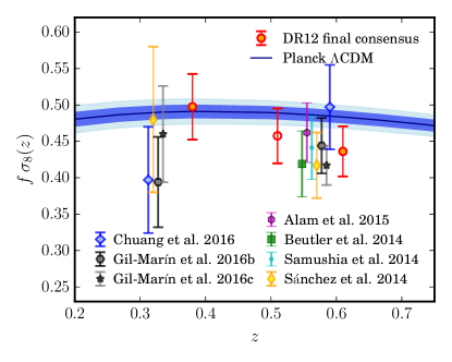
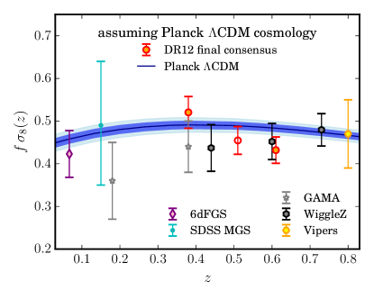
9 Cosmological parameters
9.1 Data sets
We now turn to cosmological interpretation of our results. We will use the consensus measurements, including our estimated systematic error contribution to the covariance matrix, from the BAO-only and BAO+FS columns of Table LABEL:tab:combined_BAO. In our subsequent figures and tables, the former case is simply labeled “BAO.”
Following Aubourg et al. (2015), we include the 6dFGS and SDSS MGS BAO measurements and the BOSS DR11 Ly forest BAO measurements (see Fig. 14 and §8.3). These are largely independent and have utilized similar methodologies. We opt not to include other BAO measurements, notably those from photometric clustering and from the WiggleZ survey (Blake et al., 2011a, 2012), as the volumes partially overlap BOSS and the errors are sufficiently large that a proper inclusion would not substantially affect the results. As shown in Aubourg et al. (2015), these measurements are in good agreement with those from BOSS. We note in particular the good match to the WiggleZ results, as this was a sample of strongly star-forming galaxies in marked contrast to the red massive galaxies used in BOSS. The dual-tracer opportunity was studied extensively with a joint analysis of the overlap region of WiggleZ and BOSS (Beutler et al., 2016a).
We further opt not to include other RSD measurements beyond BOSS, as they come from a variety of analysis and modelling approaches. One can see from Figure 15 that the measurements from other surveys are consistent with those from BOSS within their quoted errors, and the error bars in all cases are large enough that there are potential gains from combining multiple measurements. However, in contrast to BAO measurements, systematic errors associated with non-linear clustering and galaxy bias are a major component of the error budget in any RSD analysis, and these systematics may well be covariant from one analysis to another in a way that is difficult to quantify. Because of systematic error contributions, we do not consider it feasible to carry out a robust joint RSD analysis with other measurements.
In all cases, we combine with CMB anisotropy data from the Planck 2015 release (Planck Collaboration XIII, 2015). We use the power spectra for both temperature and polarization; in detail, we use the likelihoods plik_dx11dr2_HM_v18_TTTEEE and lowTEB for the high and low multipoles, respectively. We do not include the information from the lensing of the CMB in the 4-point correlations of the CMB temperature anisotropies. We will discuss the impact of the recent (Planck Collaboration XLVI, 2016) large-angle polarization results in §9.4.
We note that there is some mild tension between the Planck 2015 results and those from combining WMAP, SPT, and ACT (Calabrese et al., 2013; Spergel et al., 2015; Bennett et al., 2016). The Planck data set yields a mildly higher matter density , which for CDM implies a higher and and a lower . As in the DR11 results, our BOSS results for CDM fall in between these two and therefore do not prefer either CMB option. We have presented non-Planck results in Anderson et al. (2014b) and Aubourg et al. (2015) and do not repeat that here, as the sense of the differences has not changed.
Finally, for some cases, we utilize measurements of the distance-redshift relation from Type Ia supernovae (SNe) from the Joint Lightcurve Analysis (JLA, Betoule et al., 2014), which combined SNe from the SDSS-II Supernova Survey (Sako et al., 2014) and the Supernova Legacy Survey 3-year data set (Conley et al., 2011) together with local and high- data sets. The combination of SN measurements with BAO is particularly powerful for constraining the low-redshift distance scale (e.g., Mehta et al., 2012; Anderson et al., 2014b). The SNe provide a higher precision measurement of relative distance at lower redshift where the BAO is limited by cosmic volume, but the BAO provides an absolute scale that connects to higher redshift and particularly to the CMB acoustic scale at . The combination of BAO and SN data also allows an “inverse distance ladder” measurement of that uses the CMB-based calibration of but is almost entirely insensitive to the dark energy model and space curvature over the range allowed by observations (Aubourg et al., 2015).
9.2 Cosmological Parameter Results: Dark Energy and Curvature
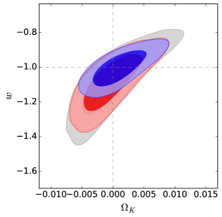
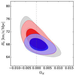
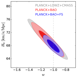
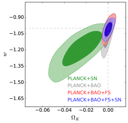
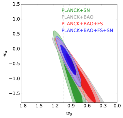
| Cosmological | Data Sets | ||||||
| Model | km/s/Mpc | ||||||
| CDM | Planck | … | … | … | |||
| CDM | Planck + BAO | … | … | … | |||
| CDM | Planck + BAO + FS | … | … | … | |||
| CDM | Planck + BAO + FS + SN | … | … | … | |||
| CDM | Planck + BAO | … | … | ||||
| CDM | Planck + BAO + FS | … | … | ||||
| CDM | Planck + BAO + FS + SN | … | … | ||||
| CDM | Planck + BAO | … | … | ||||
| CDM | Planck + BAO + FS | … | … | ||||
| CDM | Planck + BAO + FS + SN | … | … | ||||
| CDM | Planck + SN | … | |||||
| CDM | Planck + BAO | … | |||||
| CDM | Planck + BAO + FS | … | |||||
| CDM | Planck + BAO + FS + SN | … | |||||
| CDM | Planck + SN | … | |||||
| CDM | Planck + BAO | … | |||||
| CDM | Planck + BAO + FS | … | |||||
| CDM | Planck + BAO + FS + SN | … | |||||
| CDM | Planck + BAO | ||||||
| CDM | Planck + BAO + FS | ||||||
| CDM | Planck + BAO + FS + SN |
We now use these results to constrain parametrized cosmological models. We will do this using Markov Chain Monte Carlo, following procedures similar to those described in Aubourg et al. (2015), but due to use of the full power spectrum shape data we do not run any chains using that paper’s simplified “background evolution only” code. Instead, we calculate all our chains using the July 2015 version of the workhorse CosmoMC code (Lewis & Bridle, 2002). The code was minimally modified to add the latest galaxy data points and their covariance, the Ly BAO datasets, and two optional and parameters described later in the text. We use a minimal neutrino sector, with one species with a mass of 0.06 eV/ and two massless, corresponding to the lightest possible sum of neutrino masses consistent with atmospheric and solar oscillation experiments (Abe et al., 2014; Adamson et al., 2014; Gando et al., 2013), unless otherwise mentioned.
We first consider models that vary the cosmological distance scale with spatial curvature or parametrizations of the dark energy equation of state via (Chevallier & Polarski, 2001; Linder, 2003). These results are shown in Table 10 for various combinations of measurements. In all cases, the table shows the mean and 1 error, marginalized over other parameters. Of course, some parameters are covariant, as illustrated by contours in some of our figures. Our model spaces always include variations in the matter density , the baryon density , the amplitude and spectral index of the primordial spectrum, and the optical depth to recombination. However, we do not show results for these parameters as they are heavily dominated by the CMB and are not the focus of our low-redshift investigations.
We begin with the standard cosmology, the CDM model, which includes a flat Universe with a cosmological constant and cold dark matter. As is well known, CMB anisotropy data alone can constrain this model well: the acoustic peaks imply the baryon and matter density, and thereby the sound horizon, allowing the acoustic peak to determine the angular diameter distance to recombination, which in turn breaks the degeneracy between and (e.g., Spergel et al., 2003). The Planck 2015 measurements do this exquisitely well, yielding , , and (Planck Collaboration XIII, 2015).
As shown already in Figures 11 and 12, our BOSS measurements are fully consistent with the Planck CDM model results. The CDM predictions from the Planck model fits for our distance and growth observables match our measurements well, typically within 1. The combined Lyman- data do deviate at the level, which has been extensively discussed in literature (Aubourg et al., 2015; Delubac et al., 2015; Font-Ribera et al., 2014; Sahni, Shafieloo, & Starobinsky, 2014), but the overall is consistent with a minimal model. As such, the BOSS data do not require more complicated cosmologies.
As was seen in Anderson et al. (2014b) and Planck Collaboration XIII (2015), the addition of BOSS clustering data to the Planck results for the minimal CDM model does further improve the constraints on cosmological parameters. In particular, we find (0.6 per cent), , and (0.6 per cent). Adding the JLA SNe data does not further improve the errors.
We next turn to extensions that affect the distance scale, notably spatial curvature and variations in the dark energy density. In these cases, the most precise aspects of the CMB data sets suffer from a geometrical degeneracy: the CMB determines the angular diameter distance to recombination very accurately, but models that trade off low-redshift behaviour while holding this quantity fixed are more difficult to distinguish. The latest CMB data, such as from Planck, does offer ways to break the geometrical degeneracy, most effectively with gravitational lensing of the CMB, but the measurement of the low-redshift distance scale with BAO and the Alcock-Paczynski effect offers a more direct route.
As reported in Table 10, the BOSS data do this very well. Combining Planck and BOSS for the non-flat model with a cosmological constant yields a spatial curvature measurement of , confirming flatness at the level. Similarly, for the flat model with a constant dark energy equation of state, we measure a value , highly consistent with the cosmological constant. Opening both of these parameters yields a joint measurement of and . Focusing only on BAO, excluding the full-shape information, degrades this to and .
We stress that this consistency is a stringent test of the cosmological standard model. The clustering of galaxies is based on the same underlying physics as that of the CMB anisotropies. This is most obvious for the acoustic scale, but it is also true of the broadband power. We are now measuring the imprints of this physics over a wide range of redshifts, including at recombination, and finding a cosmic distance scale that returns the simple, flat, cosmological constant model while opening not one but two new degrees of freedom. The 6 per cent measurement of is a compelling demonstration of the power of galaxy clustering to measure dark energy and is an excellent counterpart to the dark energy evidence from supernovae.
Beyond this, one can consider more complicated dark energy models. However, current data do not constrain these tightly. We use here the common model. For the case with non-flat curvature, this is the fitting space for the Dark Energy Task Force Figure of Merit (Albrecht et al., 2006). We continue to find superb agreement with a flat Universe, with only 0.0028 errors on with or without inclusion of SNe. Including the SNe data does sharpen the dark energy constraints, and we find a 0.45 error on . While this constraint still allows order unity change in over , it is one of the strongest limits (perhaps the strongest) yet obtained on equation-of-state evolution.
Because of the permissive limits on evolution, the errors on at in these models are correspondingly worse. However, there is an intermediate “pivot” redshift where the errors on are minimized and where the covariance between and disappears (Albrecht et al., 2006). For the combination Planck+BAO+FS+SN in the CDM model, we find that the pivot redshift and . For CDM, we find and . We conclude that the current combination of data is able to say that Universe is flat at the level and that the dark energy was within of a cosmological constant at some epoch in the fairly recent past, but our knowledge of remains limited.
Using our constraints to compute the Dark Energy Task Force Figure of Merit (Albrecht et al., 2006), we find a result of 32.6 with SNe and 22.9 without SNe for . For comparison, the BAO-only analysis of Cuesta et al. (2016a) found a Figure of Merit of 24.3 with Planck+BAO+SN and only 8.3 without SNe. These comparisons show that the present analysis with 3 redshift bins and including the full-shape fits has notably improved the Figure of Merit. If we construct the Figure of Merit while assuming flatness (and thereby different from the Dark Energy Task Force), we find 75.4 with SNe and 44.6 without.
Our results are consistent with the distance-redshift relation from the JLA SNe. For example, adding the SNe does not significantly alter the best-fit model parameters. But the errors on a constant do continue to improve, to 0.04 in both the flat case and in the joint fit with curvature. Figure 17 shows a comparison for both CDM and CDM for galaxy clustering and SN results separately as well as the combination. We see that in CDM, the dark energy constraints even without SNe are now very tight, but the SN results are consistent and decrease the errors. It is notable that the two data sets have sharply different degeneracy directions and therefore will continue to be good partners in our cosmological constraints. For CDM, the two data sets are of more comparable power, again with different degeneracy directions, so that the combination is substantially tighter.
9.3 Cosmological Parameter Results: Dark Radiation
| Cosmological | Data Sets | ||||||
|---|---|---|---|---|---|---|---|
| Model | km/s/Mpc | ||||||
| CDM + | Planck | … | … | ||||
| CDM + | Planck + BAO + FS | … | … | ||||
| CDM + | Planck + BAO + FS + | … | … | ||||
| CDM + | Planck + BAO + FS | ||||||
| CDM + | Planck + BAO + FS + SN | ||||||
| CDM + | Planck + BAO + FS + SN + |
| Cosmological | Data Sets | [eV/] | |||||
| Model | 95% limit | ||||||
| CDM + | Planck + BAO + FS | 0.16 | … | … | … | ||
| CDM + + | Planck + BAO + FS | 0.23 | … | … | |||
| CDM + + | Planck + BAO + FS | 0.15 | … | … | |||
| CDM + + + | Planck + BAO + FS | 0.25 | … | ||||
| CDM + | Planck + BAO + FS | … | … | … | |||
| CDM + + | Planck + BAO + FS | … | … | ||||
| CDM + | Planck + BAO + FS + SN | 0.31 | … | … | … | ||
| CDM + + | Planck + BAO + FS + SN | … | … |
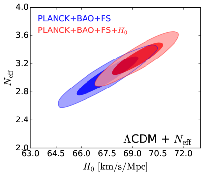
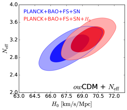
We next consider models with variations in the relativistic energy density. These are parametrized by , the effective number of neutrino species. Any new density above the 3.046 expected from standard model neutrino decoupling (Mangano et al., 2005) is assumed to be a massless species, sometimes referred to as “dark radiation” (e.g., Archidiacono et al. 2011; Calabrese et al. 2011), which may or may not result from the neutrino sector (Steigman et al., 1997; Seljak et al., 2006; Ichikawa et al., 2007; Mangano et al., 2007). Such models are important in BAO studies because the extra density in the early Universe results in a higher Hubble parameter before recombination, which in turn produces a smaller sound horizon . Since the BAO method actually measures the ratio of distance to the sound horizon, this results in smaller inferred distances and larger low-redshift Hubble parameters (Eisenstein & White, 2004; Archidiacono et al., 2011; Mehta et al., 2012; Anderson et al., 2014b; Aubourg et al., 2015). This is of substantial current interest because several high-precision direct measurements of yield values about 10 per cent higher than that inferred from combinations of Planck and BOSS BAO data (Riess et al., 2011; Freedman et al., 2012; Riess et al., 2016).
However, the Planck 2015 results appear to largely close the window for altering the sound horizon enough to reconcile the BAO+SN “inverse distance ladder” with these higher direct measurements. (Planck Collaboration XIII, 2015). The physics underlying this constraint is that Silk damping (Silk, 1968) is a diffusion process whose lengthscale depends on the square root of time, while the sound horizon depends linearly on time. The amplitude of the small-angle CMB fluctuations, when standardized by the angular acoustic scale, thereby measures the Hubble parameter at recombination and thus constrains .
Table 11 shows our parameter results for models with free , for several model and data combinations. Like Planck Collaboration XIII (2015), our chains for CDM find tight constraints, . As this central value matches that of the standard model, the central values of and move negligibly; however, the error on with free increases from 0.5 to . The error on increases only from 0.006 to 0.007, indicating that is primarily degenerate with , not . Figure 18 shows the covariance between and . If we add as a degree of freedom to the CDM model, then constraints on and are not substantially affected, as one can see by comparing the CDM lines in Tables 10 and 11. If SNe are added as an observational constraint, then CDM constraints on and remain tight, with and (see Fig. 18, right).
Riess et al. (2016) present a measurement of of (2.4 per cent), while Freedman et al. (2012) find (2.8 per cent). If we include the Riess et al. (2016) measurement as a constraint in our fits, then the preferred values of and shift upward (see Table 11 and Fig. 18), as one would expect given the disagreement between the direct and the value inferred from Planck+BAO+FS+SN. Addition of this one observation increases of the best-fit model by 8.
In the most flexible dark energy model that we consider, CDM, with we find . This can be taken as the updated value of the “inverse distance ladder” measurement assuming standard matter and radiation content from Aubourg et al. (2015). They obtained the same central value and a error bar using a flexible polynomial description of the low redshift energy density with Planck 2013, DR11 BAO, and JLA SN data.
Our inference of rests on (1) the inference of the matter density from the CMB, (2) the inference of the sound horizon from the CMB, (3) the measurement of the BAO peak in the galaxy distribution, and (4) the tracking of the expansion history from to with SNe. The good agreement between Planck 2013 and 2015 parameter determinations argues that ingredient (1) is robust. Pre-Planck CMB data implied somewhat lower values of the matter density (Calabrese et al., 2013), which would go in the direction of reconciliation (Bennett et al., 2016), but even this shift is small if one includes BAO information in addition to CMB (Anderson et al., 2014b). A substantial change in ingredient (2) appears less likely with the improved constraints from Planck 2015 discussed above. Continued improvement in the measurement of the CMB damping tail from larger aperture ground-based experiments should clarify any remaining systematic concerns and tighten the sound horizon constraints. Regarding (3), as discussed throughout the paper, we do not see a plausible way to systematically shift the BAO measurement of at the several per cent level that would be needed to substantially reduce the tension with the direct measurements. There are some rather contrived possibilities, which would be physically interesting in themselves, such as a well-tuned admixture of isocurvature perturbations that remains undetected in the CMB and yet affects fitting templates enough to distort our distance measurements, or a very large coupling of late-time galaxy bias to the the relative baryon-CDM velocity field at high redshift, which has escaped our searches due to cancellation with a second unexpected effect. Ingredient (4) is what makes our inference insensitive to the assumed dark energy model, since the SNe provide an empirical measurement of the distance ratios needed to transfer our precise BAO measurements at down to . Our analysis includes the systematic error contributions to the covariance matrix estimated by Betoule et al. (2014), and Aubourg et al. (2015) show that similar results are obtained using the Union 2 SN compilation of Suzuki et al. (2012). Our modeling adopts flexible but smooth parametric forms for the evolution of dark energy density, and it is possible that a model with more rapid low-redshift changes could shift the value of while remaining consistent with the SN data.
It is also possible that systematic errors in the direct measurement are larger than estimated by Riess et al. (2016). For example, Efstathiou (2014) presents an alternative analysis of the local data, arguing for a lower value of or , depending on the choice of primary standards. Rigault et al. (2015) argue that the dependence of the supernova luminosity after correction for light-curve fitting on the host galaxy star-formation rate causes a net calibration offset between the SNe in the Hubble flow and those with nearby Cepheid measurements; they find that this reduces by 3.3% (but see discussion by Riess et al. 2016). It is also possible that everyone’s error estimates are correct and we are simply being unlucky, e.g., if the cosmologically inferred is low and the direct measurement is high. For now, we continue to see this tension as provocative, but not conclusive. Further work that tightens the statistical errors and examines systematic uncertainties in direct measurements is clearly desirable, as this tantalizing tension could yet reveal either astrophysical or cosmological exotica.
9.4 Cosmological Parameter Results: Growth of Structure
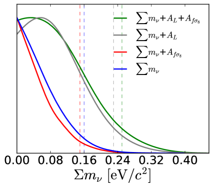
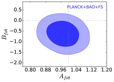
We next turn to models that assume a simpler distance scale but consider parameters to vary the growth of structure, notably through massive neutrinos or modifications of the growth rates predicted by General Relativity. These results are found in Table 12.
We start with CDM models that include an unknown total mass of the three neutrino species. In detail, we assume that all of the mass is in only one of the three weakly coupled species, but the difference between this assumption and three nearly degenerate species of the same total mass is small for our purposes. Neutrinos of sub-eV mass serve as a sub-dominant admixture of hot dark matter. Because of their substantial velocity, they fail to fall into small-scale structure at low redshift, thereby suppressing the growth of structure from recombination until today (Bond & Szalay, 1983; Hu et al., 1998). The measurement of the amplitude of the CMB anisotropy power spectrum and the optical depth to recombination implies the amplitude of the matter power spectrum at . The measurement of the expansion history along with the assumptions of GR and minimal neutrino mass then determines the amplitude of the matter power spectrum at , typically reported as . Variations in the neutrino mass then cause the expected to vary.
Measurements of the low-redshift amplitude of structure can therefore measure or limit the neutrino mass. Here, we utilize two measurements: the lensing effects on the Planck CMB anisotropy power spectrum and the BOSS RSD. Using these, we find a 95 per cent upper limit on the neutrino mass of 0.16 eV/.
We then consider how the constraints vary if one relaxes these measurements, as shown in Figure 19. We include additional nuisance parameters that scale the impact of the CMB lensing and that scales the RSD following as
| (24) |
with (chosen to be the central measurement redshift and also close to actual redshift pivot point for these two parameters). However, for the discussion of neutrinos, we keep . We note that is defined scaling the power spectrum of fluctuations, whereas varies the amplitude. This means that errors on will be double those on .
From this, we find that the measured CMB lensing power spectrum is about per cent stronger (so about 9.5 per cent on the amplitude of fluctuations) than what the CDM model would prefer, while the measured RSD is within 1 of the base level: . This means that the RSD measured in BOSS is a 6 per cent test of the expected amplitude of structure, with the central value of the measurement being slightly lower than the CDM prediction.
Interestingly, even with and varying and hence with no low-redshift measurement of the growth of structure save for a weak contribution from the Integrated Sachs Wolfe effect in the large-angle CMB anisotropies, we find a 95 per cent upper limit of eV/. This comes from the impact of the neutrino mass on the expansion history of the Universe (Aubourg et al., 2015). Essentially, the CMB inference of the balance of matter and radiation at recombination yields the density of baryons and CDM, while the measurements of the low-redshift distance scale infer a matter density that now includes the massive neutrinos as well.
Considering growth measurements one at a time, we find that including the CMB lensing effect is primarily responsible for shrinking the 95 per cent upper limit from 0.25 eV/ to 0.16 eV/. The RSD measurement alone only reaches 0.23 eV/. This is not surprising: a 1 variation of order 0.13 eV/ corresponds to a 1 per cent mass fraction of neutrinos, which yields a roughly 4 per cent change in the small-scale growth function to low redshift. This is somewhat smaller than the 6 per cent rms measurement from RSD. But the relative improvements are also being impacted by the central values of the RSD and CMB lensing inferences. RSD prefers a slightly lower normalization of small-scale power, thereby favouring a larger neutrino mass. Meanwhile, the CMB power spectrum appears to indicate a larger and hence a higher normalization of small-scale power, which pulls neutrino masses lower and makes the upper limit stronger.
As the distance scale itself is providing some constraint on the neutrino mass, we also consider fits in the CDM model. These degrade the limits to 0.31 eV/. While this is a moderate degradation, it demonstrates that the distance scale data are sufficiently good that one can simultaneously fit for expansion history and growth rate.
These limits on the neutrino mass are comparable to numerous other recent measurements. The strongest bound so far, 0.12 eV/ at 95 per cent, is presented in Palanque-Delabrouille et al. (2015) for the combination of Planck 2015 data and the one-dimensional flux power spectrum of the BOSS Lyman- forest in quasar absorption spectra. Recent attempts to combine the galaxy power spectrum with with Planck 2015 data (Giusarma et al., 2016; Cuesta et al., 2016b) produce bounds between 0.25 and 0.30 eV/, depending on the power spectrum datasets used and the number of massive neutrino states assumed in the analysis (or 0.20 eV/ if a compilation of recent BAO data is used instead of the power spectrum). This can be brought further down to 0.12 eV/ if a Hubble constant prior from direct measurements is imposed additionally. However, the combination of cosmological datasets in tension with each other can drive a spurious neutrino mass signal, so it is important to address these issues before naively interpreting as a neutrino mass detection a signature of systematic effects. For example Beutler et al. (2014b) showed that a somewhat large neutrino mass of eV/ is favoured when combining CMASS Data Release 11 with WMAP9 data. A similar result is confirmed when combining CMASS DR11 with Planck 2013 if the lensing parameter is marginalized out. If is not marginalized over, this is not the case, as reported in the Planck paper. Finally, the identification and removal of systematic effects on large angular scales in the polarization data of Planck has resulted in a stronger bound on neutrino mass from CMB data alone, placing a limit of 0.59 eV/ without polarization and 0.34 eV/ with polarization (Planck Collaboration XLVI, 2016).
Instead of explaining any variations in the amplitude of structure by a non-minimal neutrino mass, one could instead view it as a test of the growth rate of structure under General Relativity. In this sense these nuisance parameters can be regarded as a test similar to that usually carried out using the phenomenological parameter (Wang & Steinhardt 1998; Linder et al. 2007). This has the advantage of being independent of the model of structure formation, simple to interpret and directly measured by the data, at the expense of not constraining any concrete theories of modified gravity. Again for CDM, we find ; that is, via the BOSS RSD measurement, we infer to be within 6 per cent of the CDM prediction. While this level of precision on can be achieved by several methods, such as cluster abundances or weak lensing, the measurement of the time derivative of the growth function is harder to access with methods that measure only the single-redshift amplitude of the power spectrum.
Extending the model to include a redshift-dependent variation , we find . This is a mild indication of evolution, with the ratio of the measured to the predicted value decreasing toward higher redshift. The results for LCDM are visualized in Figure 20. This is consistent with the trend from Figure 12. As this slope is only non-zero at 1.5, we do not regard this as a statistically significant detection of this second parameter. We conclude that our RSD measurements indicate that structure is growing in a manner consistent with General Relativity even in the epoch dominated by dark energy.
Table 12 further shows that the constraints on and change negligibly if we extend the expansion history to the CDM model. This implies that the distance scale information is setting the GR prediction for to a level that is well better than we can measure it with RSD.
We note that the Planck collaboration has recently concluded (Planck Collaboration XLVI, 2016) that the optical depth to reionization inferred from large-angle -mode polarization is , about 30 per cent less than the value of that results from the Planck Collaboration XIII (2015) likelihood that we use here. This has the consequence of decreasing the amplitude of structure at recombination by 2 per cent, which in turn reduces the prediction of at low redshift by the same amount. This will not affect our errors on , but would increase the central value by 2 per cent. It will push the neutrino masses toward lower values, slightly reducing our upper limits (as well as any others based on Planck Collaboration XIII 2015), as there is less room for a decrement of low-redshift power caused by hot dark matter.
RSD measurements are only one part of an active current debate about the amplitude of low-redshift structure. Measurements of cosmic shear and galaxy-galaxy lensing (Heymans et al., 2013; Mandelbaum et al., 2013; MacCrann et al., 2015; Hildebrandt et al., 2016) and of cluster abundances (Vikhlinin et al., 2009; Rozo et al., 2010; Planck Collaboration XX, 2014; Planck Collaboration XXIV, 2015) have often yielded notably lower amplitudes than the Planck predictions in CDM or the Planck measurement of the lensing of the CMB from 4-point correlations (Planck Collaboration XIII, 2015). The tension can be up to 10 per cent in the amplitude and 2-3 per measurement, although there are cosmic shear measurements (Jee et al., 2013) and cluster mass calibrations (Mantz et al., 2015) that argue for a higher amplitude. The small-scale clustering of the Lyman forest provides another data point, more in line with the higher Planck prediction. Our BOSS RSD measurement falls in the middle of the dispute, with being consistent with the Planck prediction but also with the lower values. For example, our LCDM chain with varying finds , so the RSD measurement itself would favor a value per cent lower, e.g., . This might be compared, for example, to the measurement from Hildebrandt et al. (2016). While this is not a provocative position, we note that all of these routes to the low-redshift amplitude depend on controlling some thorny systematic or modelling issue. It is therefore fortunate that there are multiple viable methods as we attempt to reach sub-percent precision.
10 Conclusion
We have presented measurements of the cosmological distance-redshift relation as well as the growth rate of large-scale structure using an extensive analysis of the clustering of galaxies from the completed SDSS-III Baryon Oscillation Spectroscopic Survey. The final sample includes 1.2 million massive galaxies over 9382 deg2 covering , making it the largest spectroscopic galaxy sample yet utilized for cosmology. We split this sample into three partially overlapping redshift bins, each large enough for clear detections of the baryon acoustic oscillations, so as to study the expansion history and evolving structure formation of the Universe. These bins have effective redshifts of 0.38, 0.51, and 0.61.
The consensus results of this paper are the synthesis of the results of several companion papers studying this sample with a variety of methods and with the support of large suites of mock catalogues. Beutler et al. (2016b); Ross et al. (2016); Vargas-Magaña et al. (2016) have measured the distance scale by localizing the BAO feature and estimated systematic uncertainties in these measurements, while Beutler et al. (2016c); Grieb et al. (2016); Sánchez et al. (2016a); Satpathy et al. (2016) have modelled the RSD signature in the full-shape of the clustering measurements to add structure growth constraints and improve AP effect measurements. Studies of high-resolution mock samples described in Tinker et al. (2016) have enabled the estimate of systematic uncertainties of the structure growth measurements. Sánchez et al. (2016b) describes how the results of the independent analyses have been combined into one 9-dimensional Gaussian likelihood that includes the covariance between our 3 redshift slices and between our pre-reconstruction and post-reconstruction analyses.
These results represent the first instance in which post-reconstruction BAO distance measurements have been combined with structure growth measurements obtained by modelling the RSD signature. We expect this will be the standard in future analyses, e.g., with data from the DESI experiment, and that methods will be further improved to simultaneously model post-reconstruction BAO information and RSD signatures (White, 2015).
The consensus likelihood presented here is then used to measure parametrized models of cosmology, including variations in dark energy, spatial curvature, neutrino masses, extra relativistic density, and modifications of gravity. In all cases, we combine our BOSS measurements with those from the power spectra of CMB temperature and polarization anisotropies from Planck Collaboration XIII (2015). The common physics and theoretical model underlying the phenomena of CMB anisotropies and late-time large-scale structure make this an extremely powerful cosmological probe. We now have compelling measurements of the baryon acoustic oscillations at a variety of redshifts, including the exquisite detection at , demonstrating the commonality of the physical basis for structure formation from recombination to today. The standard ruler provided by the BAO is a clear and robust marker of the distance-redshift relation. Moreover, the expansion history this implies is in excellent agreement with the inference of the matter-radiation equality from the CMB acoustic peak heights. This is a remarkable qualitative success of modern cosmology.
Turning to our quantitative results, we highlight the following conclusions:
1) The results of the seven data analyses using a variety of methodologies are demonstrated to be consistent at the level expected based on analysis of mock galaxy samples. Notably this includes four different analyses of redshift-space distortions and the Alcock-Paczynski effect, the models of which were validated on a variety of N-body simulations and mock catalogues. Our measurements include an estimate of systematic uncertainties, but we expect we are limited by our statistical uncertainties.
2) We measure the Hubble parameter to better than 2.4 per cent and the angular diameter distance to better than 1.5 per cent accuracy in each of our redshift bins. When combined, the measurements represent a 1.0 per cent constraint on the transverse distance scale and a 1.6 per cent constraint on the radial distance scale.
3) From the anisotropy of redshift-space clustering, we measure the amplitude of the peculiar velocity, parametrized as , to 9.2 per cent or better than precision in each redshift bin. In total, we find a 6 per cent measurement of a bulk shift of relative to the flat CDM model.
We find no tensions in our combined measurements when they are compared to the predictions of the Planck best-fit CDM model.
4) Combining with the Planck 2015 power spectrum likelihood, we find no preference for a model that includes additional parameters beyond the vanilla spatially flat CDM model. This remains true when combined with JLA SNe data.
5) In the simplest spatially flat CDM model, our data moderately tightens the errors from Planck alone, yielding and Allowing extra relativistic density loosens the errors but does not notably shift the central value, yielding , , and .
6) Models simultaneously varying a constant dark energy equation of state parameter and spatial curvature are tightly constrained. Using Planck and BOSS data alone yields and , in tight agreement with the flat CDM model despite having opened two new degrees of freedom. Adding JLA SNe improves the dark energy result to while also yielding .
7) Flat models with a time-variable equation of state are less well constrained, with finding without SNe and with SNe. We do continue to find tight errors on at a pivot redshift, .
8) We find tight and stable limits on for all cases. For example, for our most general CDM model, we find with SNe. We also find for the CDM model with extra relativistic species. As such, our results do nothing to reduce the tension with the direct measurements of that have found higher values, such as the of Riess et al. (2016). Whether this remains to be explained as some combination of statistical and systematic errors or is an indication of a breakdown of the flat CDM model is an enticing open question; our results indicate that curvature, smooth evolution of dark energy at low redshift, or extra pre-recombination energy as parameterized by are not enough to resolve the discrepancy.
9) We place strong constraints on the sum of the neutrino masses. The 95 per cent upper limit is 0.16 eV; this can be compared to the minimum of 0.06 eV. Removing any growth of structure information (i.e., information from our data set and CMB lensing information from Planck), we find the upper limit increases to 0.25 eV, with the information coming primarily from the effect of the neutrino mass on the expansion history.
10) Alternatively, if one interprets the measurement of as a test of the GR prediction for the growth rate of large-scale structure given the measured expansion history, we find a rescaling of , which is a 6 per cent measurement consistent with GR. Testing for redshift evolution, we find a mild preference, about 1.5, for evolution compared to the value predicted by GR. We do not regard this preference as statistically significant.
This work represents the culmination of large-scale structure goals of the BOSS galaxy survey. The survey fulfilled its experimental design and produced a three-dimensional map of the structure of the Universe over a volume of 18.7 Gpc3 with sufficient sampling to be dominated by sample variance on scales modelled by cosmological linear theory. BOSS showed that the BAO feature exists in the distribution of galaxies to greater than 10 significance and that the subsequent recovery of the acoustic scale allows robust and precise measurements of angular diameter distance to and the expansion rate at the redshift of the galaxies. These BAO distance measurements form a compelling low-redshift complement to the beautifully detailed view of early structure gained from CMB observations. The ability to observe a single well-modelled physical effect from recombination until today is a great boon for cosmology and now underlies much of cosmological parameter estimation. Further, our analyses have extended the use of the anisotropic galaxy clustering signatures of RSD and the Alcock-Paczynski effect to the unprecedented size of the BOSS sample, producing robust measurements of the expansion history and the rate of structure growth. We believe that BOSS has marked an important cosmological milestone, combining precise clustering measurements of an enormous volume with detailed modelling from cosmological simulations and extensive observations of the primary CMB anisotropies to produce a persuasive jump in the quality of our cosmological inferences from large-scale structure and a firm platform for the search for extensions to the standard cosmological model. We look forward to seeing this program extended with the coming decade of large spectroscopic surveys.
Acknowledgements
SSA, JNG, and AGS acknowledge support from the Trans-regional Collaborative Research Centre TR33 ‘The Dark Universe’ of the German Research Foundation (DFG). FB acknowledges support from the UK Space Agency through grant ST/N00180X/1. ASB acknowledges support from the U.S. Department of Energy, Office of Science, Office of High Energy Physics under Award Number DE-SC0010331. AJC is supported by the European Research Council under the European Community’s Seventh Framework Programme FP7-IDEAS-Phys.LSS 240117 and the Spanish MINECO under projects AYA2014-58747-P and MDM-2014-0369 of ICCUB (Unidad de Excelencia ’María de Maeztu’). KSD acknowledges support from the U.S. Department of Energy, Office of Science, Office of High Energy Physics under Award Number DE-SC0009959. DJE acknowledges support from the U.S. Department of Energy, Office of Science, Office of High Energy Physics under Award Number DE-SC0013718. HGM acknowledges Labex ILP (reference ANR-10-LABX-63) part of the Idex SUPER, and received financial state aid managed by the Agence Nationale de la Recherche, as part of the programme Investissements d’avenir under the reference ANR-11-IDEX-0004-02. WJP acknowledges support from the UK Science and Technology Facilities Research Council through grants ST/M001709/1 and ST/N000668/1, the European Research Council through grant 614030 Darksurvey, and the UK Space Agency through grant ST/N00180X/1. NPR acknowledges support from the STFC and the Ernest Rutherford Fellowship scheme. GR acknowledges support from the National Research Foundation of Korea (NRF) through NRF-SGER 2014055950 funded by the Korean Ministry of Education, Science and Technology (MoEST), and from the faculty research fund of Sejong University. H-JS acknowledges support from the U.S. Department of Energy, Office of Science, Office of High Energy Physics under Award Number DE-SC0014329. RT acknowledges support from the Science and Technology Facilities Council via an Ernest Rutherford Fellowship (grant number ST/K004719/1).
Funding for SDSS-III has been provided by the Alfred P. Sloan Foundation, the Participating Institutions, the National Science Foundation, and the U.S. Department of Energy Office of Science. The SDSS-III web site is http://www.sdss3.org/.
SDSS-III is managed by the Astrophysical Research Consortium for the Participating Institutions of the SDSS-III Collaboration including the University of Arizona, the Brazilian Participation Group, Brookhaven National Laboratory, University of Cambridge, Carnegie Mellon University, University of Florida, the French Participation Group, the German Participation Group, Harvard University, the Instituto de Astrofisica de Canarias, the Michigan State/Notre Dame/JINA Participation Group, Johns Hopkins University, Lawrence Berkeley National Laboratory, Max Planck Institute for Astrophysics, Max Planck Institute for Extraterrestrial Physics, New Mexico State University, New York University, Ohio State University, Pennsylvania State University, University of Portsmouth, Princeton University, the Spanish Participation Group, University of Tokyo, University of Utah, Vanderbilt University, University of Virginia, University of Washington, and Yale University.
Based on observations obtained with Planck (http://www.esa.int/Planck), an ESA science mission with instruments and contributions directly funded by ESA Member States, NASA, and Canada.
This research used resources of the National Energy Research Scientific Computing Center, a DOE Office of Science User Facility supported by the Office of Science of the U.S. Department of Energy under Contract No. DE-AC02-05CH11231.
References
- Abazajian et al. (2004) Abazajian, K., Adelman-McCarthy, J. K., Agüeros, M. A., et al. 2004, AJ, 128, 502
- Abe et al. (2014) Abe, K., et al. 2014, PRL, 112, 1818
- Acacia et al. (2015) Acacia, R.
- Adamson et al. (2014) Adamson, P., et al. 2014, PRL, 112, 1918
- Aihara et al. (2011) Aihara, H., Allende Prieto, C., An, D., et al. 2011, ApJS, 193, 29
- Alam et al. (2015a) Alam, S., Albareti, F. D., Allende Prieto, C., et al. 2015, ApJS, 219, 12
- Alam et al. (2015b) Alam, S., Ho, S., Vargas-Magaña, M., & Schneider, D. P. 2015, MNRAS, 453, 1754
- Albrecht et al. (2006) Albrecht A., et al., 2006, arXiv:astro-ph/0609591
- Alcock & Paczynski (1979) Alcock C., Paczynski B., 1979, Nature, 281, 358.
- Amendola et al. (2016) Amendola, L., et al. 2016, arXiv:1606.00180
- Anderson et al. (2012) Anderson, L., Aubourg, E., Bailey, S., et al. 2012, MNRAS, 427, 3435
- Anderson et al. (2014a) Anderson, L., Aubourg, E., Bailey, S., et al. 2014, MNRAS, 439, 83
- Anderson et al. (2014b) Anderson, L., Aubourg, E., Bailey, S., et al. 2014, MNRAS, 441, 24
- Archidiacono et al. (2011) Archidiacono, M., Calabrese, E. & Melchiorri, A., 2011, Phys. Rev. D, 84, 123008
- Astier & Pain (2012) Astier, P., & Pain, R. 2012, 13, 521
- Aubourg et al. (2015) Aubourg, É., Bailey, S., Bautista, J. E., et al. 2015, Phys. Rev. D, 92, 123516
- Barkana & Loeb (2011) Barkana, R., & Loeb, A., 2011, MNRAS, 415, 3113
- Bennett et al. (2013) Bennett, C. L., et al. 2013, ApJS, 208, 20
- Bennett et al. (2016) Bennett, C.L., Larson, D., Weiland, J.L., & Hinshaw, G., 2014, ApJ, 794, 135
- Betoule et al. (2014) Betoule, M., Kessler, R., Guy, J., et al. 2014, A&A, 568, A22
- Beutler et al. (2011) Beutler F., et al. 2011, MNRAS, 416, 3017
- Beutler et al. (2012) Beutler F., et al. 2012, MNRAS, 423, 3430
- Beutler et al. (2014a) Beutler F. et al., 2014a, MNRAS, 443, 1065
- Beutler et al. (2014b) Beutler, F., et al., 2014b, MNRAS, 444, 3501
- Beutler et al. (2016a) Beutler, F., Blake, C., Koda, J., Marín, F.A., Seo, H., & Cuesta A.J., 2016a, MNRAS, 455, 3230
- Beutler et al. (2016b) Beutler, F. et al. 2016b, submitted
- Beutler et al. (2016c) Beutler, F. et al. 2016c, submitted
- Bianchi et al. (2015) Bianchi D., Gil-Marin H., Ruggeri R. and Percival W. J., 2015, MNRAS, 453, 11
- Blake et al. (2011a) Blake C., et al., 2011, MNRAS, 418, 1707
- Blake et al. (2011b) Blake C., et al., 2011b, MNRAS, 418, 1725
- Blake et al. (2012) Blake C., et al., 2012, MNRAS, 425, 405
- Blake et al. (2013) Blake, C., Baldry, I. K., Bland-Hawthorn, J., et al. 2013, MNRAS, 436, 3089
- Blake & Glazebrook (2003) Blake, C., & Glazebrook, K. 2003, ApJ, 594, 665
- Blanchard (2010) Blanchard, A. 2010, A& A Rv, 18, 595
- Blazek et al. (2016) Blazek, J., McEwen, J. & Hirata, C., 2016, Phys. Rev. Letters, 116, 121303
- Bolton et al. (2012) Bolton A., et al., 2012, AJ, 144, 144
- Bond & Szalay (1983) Bond, J.R., & Szalay, A.S., 1983, ApJ, 274, 443
- Burden, Percival & Howlett (2015) Burden, A., Percival, W. J., Howlett, C., 2015, MNRAS, 453, 456
- Busca et al. (2013) Busca, N.G., et al., 2013, A&A, 552, 96
- Calabrese et al. (2011) Calabrese, E., Huterer, D., Linder, E. V., Melchiorri, A., & Pagano, L. 2011, Phys Rev D, 83, 123504
- Calabrese et al. (2013) Calabrese, E., et al., 2013, PRD, 87, 3012
- Carlson et al. (2013) Carlson, J., Reid, B., & White, M. 2013, MNRAS, 429, 1674
- Chevallier & Polarski (2001) Chevallier, M., & Polarski, D. 2001, International Journal of Modern Physics D, 10, 213
- Chuang & Wang (2012) Chuang, C.-H., & Wang, Y. 2012, MNRAS, 426, 226
- Chuang et al. (2013a) Chuang C.-H. et al., 2013, MNRAS, 433, 3559
- Chuang & Wang (2013b) Chuang, C.-H., & Wang, Y. 2013, MNRAS, 431, 2634
- Chuang et al. (2015) Chuang, C.-H., Zhao, C., Prada, F., et al. 2015, MNRAS, 452, 686
- Chuang et al. (2016) Chuang, C.. et al. 2016, submitted
- Cole, Fisher, & Weinberg (1994) Cole, S., Fisher, K. B., & Weinberg, D. H. 1994, MNRAS, 267, 785
- Cole, Fisher, & Weinberg (1995) Cole, S., Fisher, K. B., & Weinberg, D. H. 1995, MNRAS, 275, 515
- Cole et al. (2005) Cole, S., Percival, W. J., Peacock, J. A., et al. 2005, MNRAS, 362, 505
- Colless et al. (2003) Colless M., et al., 2003, astro-ph/0306581
- Conley et al. (2011) Conley, A., et al., 2011, ApJS, 192, 1
- Copeland, Sami, & Tsujikawa (2006) Copeland, E. J., Sami, M., & Tsujikawa, S. 2006, International Journal of Modern Physics D, 15, 1753
- Cuesta et al. (2016a) Cuesta, A. J., Vargas-Magaña, M., Beutler, F., et al. 2016, MNRAS, 457, 1770
- Cuesta et al. (2016b) Cuesta, A. J., Niro, V., Verde, L., 2016, PDU, 13, 77
- Dalal et al. (2010) Dalal, N., Pen, U.-L., & Seljak, U. 2010, JCAP, 11, 007
- Das et al. (2014) Das, S., et al. 2014, JCAP, 4, 014
- Dawson et al. (2013) Dawson K. S., et al., 2013, AJ, 145, 10
- de Bernardis et al. (2000) de Bernardis, P., et al. 2000, Nature, 404, 955
- Delubac et al. (2015) Delubac, T., Bautista, J. E., Busca, N. G., et al. 2015, A&A, 574, A59
- de la Torre and Guzzo (2012) de la Torre, S. and Guzzo, L., 2012, MNRAS, 427, 327
- de la Torre et al. (2013) de la Torre, S., Guzzo, L,; Peacock, J. A., et al. 2013, A&A, 557, A54
- Doi et al. (2010) Doi M., et al., 2010, AJ, 139, 1628
- Doroshkevich et al. (1978) Doroshkevich A.G., Zel’dovich Ya.B., Sunyaev R.A., 1978 Soviet Astronomy, 22, 523
- Efstathiou (2014) Efstathiou, G., 2014, MNRAS, 440, 1138
- Efstathiou, Sutherland, & Maddox (1990) Efstathiou, G., Sutherland, W. J., & Maddox, S. J. 1990, Nature, 348, 705
- Eisenstein et al. (2001) Eisenstein, D. J., et al. 2001, AJ, 122, 2267
- Eisenstein & Hu (1998) Eisenstein D.J., Hu W., 1998, ApJ, 496, 605
- Eisenstein, Hu, & Tegmark (1998) Eisenstein, D. J., Hu, W., & Tegmark, M. 1998, ApJ, 504, L57
- Eisenstein & White (2004) Eisenstein D.J., & White, M., 2004, PRD, 70, 3523
- Eisenstein et al. (2005) Eisenstein, D. J., Zehavi, I., Hogg, D. W., et al. 2005, ApJ, 633, 560
- Eisenstein et al. (2007) Eisenstein, D. J., Seo, H.-J., Sirko, E., & Spergel, D. N. 2007, ApJ, 664, 675
- Eisenstein et al. (2007b) Eisenstein D.J., Seo H.-J., White M., 2007b, ApJ, 664, 660
- Eisenstein et al. (2011) Eisenstein D. J., et al., 2011, AJ, 142, 72
- Favole et al. (2015) Favole, G., McBride, C. K., Eisenstein, D. J., et al. 2015, arXiv:1506.02044
- Feldman, Kaiser, & Peacock (1994) Feldman, H. A., Kaiser, N., & Peacock, J. A. 1994, ApJ, 426, 23
- Font-Ribera et al. (2014) Font-Ribera, A., Kirkby, D., Busca, N., et al. 2014, JCAP, 5, 027
- Freedman et al. (2012) Freedman, W. L., et al., 2012, ApJ, 758, 24
- Frieman, Turner, & Huterer (2008) Frieman, J. A., Turner, M. S., & Huterer, D. 2008, ARA&A, 46, 385
- Fukugita et al. (1996) Fukugita M., et al., 1996, AJ, 111, 1748
- Gando et al. (2013) Gando, A., et al., 2013, PRD, 88, 330
- Gaztañaga et al. (2009) Gaztañaga, E., Cabré, A., & Hui, L. 2009, MNRAS, 399, 1663
- George et al. (2015) George, E. M., et al. 2015, ApJ, 799, 177
- Gil-Marín et al. (2016a) Gil-Marín, H., Percival, W. J., Cuesta, A. J., et al. 2016, MNRAS,
- Gil-Marín et al. (2016b) Gil-Marín, H., Percival, W. J., Brownstein, J. R., et al. 2016, MNRAS,
- Gil-Marín et al. (2016c) Gil-Marín, H., et al. 2016, arXiv:1606.00439
- Giusarma et al. (2016) Giusarma, E.; Gerbino, M.; Mena, O., et al. 2016, arXiv:1605.04320
- Grieb et al. (2015) Grieb, J. N., Sánchez, A. G.; Salazar-Albornoz, S., Dalla Vecchia, C., 2016, MNRAS, 457, 1577
- Grieb et al. (2016) Grieb, J. et al., 2016, submitted
- Gunn et al. (1998) Gunn J.E., et al., 1998, AJ, 116, 3040
- Gunn et al. (2006) Gunn J.E., et al., 2006, AJ, 131, 2332
- Guzzo et al. (2008) Guzzo L. et al., 2008, Nature, 451, 541
- Hanany et al. (2000) Hanany, S., et al. 2000, ApJ, 545, L5
- Hartlap et al. (2006) Hartlap J., Simon P., Schneider P., 2007, Astron.Astrophys., 464, 399
- Hawkins et al. (2003) Hawkins E. et al., 2003, MNRAS, 346, 78
- Heymans et al. (2013) Heymans, C., et al., 2013, MNRAS 432, 2433
- Hildebrandt et al. (2016) Hildebrandt, H., et al., 2016, MNRAS, submitted; arXiv:1606.05338
- Howlett et al. (2015) Howlett, C. et al., 2015, MNRAS, 449, 848 2015MNRAS.449..848H
- Hu et al. (1998) Hu, W., Eisenstein, D.J., & Tegmark, M., 1998, PRL, 80, 5255
- Huterer et al. (2015) Huterer, D., et al. 2015, Astroparticle Physics, 63, 23
- Ichikawa et al. (2007) Ichikawa K., Kawasaki M., Takahashi F., 2007, J. Cosmol. Astropart. Phys., 5, 7
- Jain & Khoury (2010) Jain, B., & Khoury, J. 2010, Annals of Physics, 325, 1479
- Jee et al. (2013) Jee, M.J., Tyson, J.A., Schneider, M.D., Wittman, D., Schmidt, S., & Hilbert, S., 2013, ApJ, 765, 74
- Joyce, Lombriser, & Schmidt (2016) Joyce, A., Lombriser, L., & Schmidt, F. 2016, arXiv:1601.06133
- Kaiser (1987) Kaiser N., 1987, MNRAS, 227, 1
- Kazin et al. (2012) Kazin, E. A. and Sánchez, A. G. and Blanton, M. R., 2012, MNRAS, 419, 3223
- Kim et al. (2015) Kim, A. G., et al. 2015, Astroparticle Physics, 63, 2
- Kitaura et al. (2014) Kitaura F.-S., Yepes G., Prada F., 2014, MNRAS, 439, L21
- Kitaura et al. (2016) Kitaura, F.-S., Rodríguez-Torres, S., Chuang, C.-H., et al. 2016, MNRAS, 456, 4156
- Kirkby et al. (2013) Kirkby, D., et al., 2013, JCAP, 3, 24
- Krauss & Turner (1995) Krauss, L. M., & Turner, M. S. 1995, General Relativity and Gravitation, 27, 1137
- Landy & Szalay (1993) Landy, Stephen D., & Szalay, Alexander S., 1993, ApJ, 412, 64
- Lesgourgues & Pastor (2006) Lesgourgues, J., & Pastor, S. 2006, Phys. Rep., 429, 307
- Lewis & Bridle (2002) Lewis, A. & Bridle, S. 2002, Phys. Rev. D, 66, 103511
- Linder (2003) Linder E. V., 2003, PhRvD, 90, 091301
- Linder et al. (2007) Linder E. V., Cahn R. N., 2007, Astropart. Phys., 29, 336
- Loveday et al. (1996) Loveday, J., Efstathiou, G., Maddox, S. J., & Peterson, B. A. 1996, ApJ, 468, 1
- LSST Science Collaboration et al. (2009) LSST Science Collaboration, et al. 2009, LSST Science Book, Version 2.0, arXiv:0912.0201
- Lupton et al. (2001) Lupton R., Gunn J.E., Ivezic Z., Knapp G., Kent S., 2001, Astronomical Data Analysis Software and Systems X, v.238, 269.
- MacCrann et al. (2015) MacCrann N., Zuntz, J., Bridle, S., Jain, B., Becker, M. R., 2015, MNRAS, 451, 2877
- Mandelbaum et al. (2013) Mandelbaum, R., Slosar, A., Baldauf, T., Seljak, U., Hirata, C.M., Nakajima, R., Reyes, R., Smith, R. E., 2013, MNRAS 432, 1544
- Manera et al. (2015) Manera, M., Samushia, L., Tojeiro, R., et al. 2015, MNRAS, 447, 437
- Mangano et al. (2005) Mangano G., et al. 2005, PLB, 729, 221
- Mangano et al. (2007) Mangano G., Melchiorri A., Mena O., Miele G., Slosar A., 2007, J. Cosmol. Astropart. Phys., 3, 6
- Mantz et al. (2015) Mantz A.B. et al., 2015, MNRAS, 446, 2205
- Mehta et al. (2011) Mehta, K. T., Seo, H.-J., Eckel, J., Eisenstein, D. J., Metchnik, M., Pinto, P., & Xu, X. 2011, ApJ, 734, 94
- Mehta et al. (2012) Mehta K., et al., 2012, MNRAS, 427, 2168
- Meiksin, White & Peacock (1999) Meiksin A., White M., Peacock J.A., 1999, MNRAS 304, 851
- Netterfield et al. (1997) Netterfield, C. B., Devlin, M. J., Jarosik, N., Page, L., & Wollack, E. J. 1997, ApJ, 474, 47
- Noh, White, & Padmanabhan (2009) Noh, Y., White, M., & Padmanabhan, N. 2009, Phys Rev D, 80, 123501
- Oka et al. (2014) Oka A., Saito S., Nishimichi T., Taruya A., Yamamoto K., 2014, MNRAS, 439, 2515
- Okumura et al. (2008) Okumura, T., Matsubara, T., Eisenstein, D. J., Kayo, I., Hikage, C., Szalay, A. S., & Schneider, D. P. 2008, ApJ, 676, 889-898
- Ostriker & Steinhardt (1995) Ostriker, J. P., & Steinhardt, P. J. 1995, Nature, 377, 600
- Patej & Eisenstein (2016) Patej, A., & Eisenstein, D. 2016, MNRAS, 460, 1310
- Padmanabhan et al. (2007) Padmanabhan, N., et al. 2007, MNRAS, 378, 852
- Padmanabhan et al. (2008) Padmanabhan N., et al., 2008, ApJ, 674, 1217
- Padmanabhan & White (2008) Padmanabhan, N., & White, M. 2008, Phys. Rev. D, 77, 123540
- Padmanabhan, White, & Cohn (2009) Padmanabhan, N., White, M., & Cohn, J. D. 2009, Phys Rev D, 79, 063523
- Padmanabhan & White (2009) Padmanabhan, N., & White, M. 2009, Phys. Rev. D, 80, 063508
- Padmanabhan et al. (2012) Padmanabhan et al., 2012, MNRAS, 427, 2132
- Palanque-Delabrouille et al. (2015) Palanque-Delabrouille N., Yèche C., Baur J., et al. 2015, JCAP, 11, 11
- Peacock et al. (2001) Peacock J. A. et al., 2001, Nature, 410, 169
- Peebles & Yu (1970) Peebles P.J.E., Yu J.T., 1970, ApJ, 162, 815
- Pellejero-Ibañez et al. (2016) Pellejero-Ibañez, M., Chuang, C.-H., Rubiño-Martín, J. A., et al. 2016, submitted
- Percival et al. (2001) Percival W. J., 2001, MNRAS, 327, 1297
- Percival et al. (2004a) Percival W. J., Verde, L., & Peacock, J. A. 2004a, MNRAS, 347, 645
- Percival et al. (2004b) Percival W. J., et al., 2004b, MNRAS, 353, 1201
- Percival et al. (2007) Percival W.J., et al., 2007, MNRAS, 381, 1053
- Percival & White (2009) Percival, W. J., & White, M. 2009, MNRAS, 393, 297
- Percival et al. (2010) Percival W.J., et al., 2010, MNRAS, 401, 2148
- Percival et al. (2014) Percival, W. J., Ross, A. J., Sánchez, A. G., et al. 2014, MNRAS, 439, 2531
- Perlmutter et al. (1999) Perlmutter, S., Aldering, G., Goldhaber, G., et al. 1999, ApJ, 517, 565
- Pier et al. (2003) Pier J.R., et al., 2003, AJ, 125, 1559
- Planck Collaboration I (2015) Planck Collaboration I, Ade P.A.R., et al., 2015, arXiv:1502.01582
- Planck Collaboration XX (2014) Planck Collaboration XX, Ade P.A.R., et al., 2014, A&A, 571, A20
- Planck Collaboration XXIV (2015) Planck Collaboration XXIV, Ade P.A.R., et al., 2015, arXiv:1502.01597
- Planck Collaboration XIII (2015) Planck Collaboration XIII, Ade, P. A. R., et al. 2015, arXiv:1502.01589
- Planck Collaboration XLVI (2016) Planck Collaboration XLVI, Ade, P. A. R., et al. 2016, arXiv:1605.02985
- Reid et al. (2012) Reid B.A., et al., 2012, MNRAS, 426, 2719
- Reid et al. (2014) Reid B. A., Seo H.-J., Leauthaud A., Tinker J. L., White M., 2014, MNRAS, 444, 476
- Reid et al. (2016) Reid, B., Ho, S., Padmanabhan, N., et al. 2016, MNRAS, 455, 1553
- Riebe et al. (2013) Riebe, K., Partl, A. M., Enke, H., et al. 2013, Astronomische Nachrichten, 334, 691
- Riess et al. (1998) Riess, A. G., Filippenko, A. V., Challis, P., et al. 1998, AJ, 116, 1009
- Riess et al. (2011) Riess A. G., et al., 2011, ApJ, 730, 119
- Riess et al. (2016) Riess A. G., et al., 2016, arXiv:1604.01424
- Rigault et al. (2015) Rigault, M., et al., 2015, ApJ, 802, 1
- Ross et al. (2012) Ross, A. J., Percival, W. J., Sánchez, A. G., et al. 2012, MNRAS, 424, 564
- Ross et al. (2014) Ross, A. J., Samushia, L., Burden, A., et al. 2014, MNRAS, 437, 1109
- Ross et al. (2015) Ross, A. J., Samushia, L., Howlett, C., et al. 2015, MNRAS, 449, 835
- Ross et al. (2015) Ross, A. J., Percival, W., & Manera, M., 2015, MNRAS, 451, 1331
- Ross et al. (2016) Ross, A. J., et al. 2016, submitted
- Rozo et al. (2010) Rozo, E., et al., 2010, ApJ 708, 645
- Sachs & Wolfe (1967) Sachs, R. K., & Wolfe, A. M. 1967, ApJ, 147, 73
- Sahni, Shafieloo, & Starobinsky (2014) Sahni, V., Shafieloo, A., & Starobinsky, A. A. 2014, ApJ, 793, L40
- Sako et al. (2014) Sako, M., et al., 2014, arXiv:1401.3317
- Salazar-Albornoz et al. (2016) Salazar-Albornoz, S., Sánchez, A. G., Grieb, J. N., et al., submitted
- Samushia et al. (2013) Samushia L., et al., 2013, MNRAS, 429, 1514
- Samushia et al. (2014) Samushia, L., et al., 2014, MNRAS, 439, 3504
- Sánchez et al. (2013) Sánchez A. G. et al., 2013, MNRAS, 433, 1202
- Sánchez et al. (2014) Sánchez A. G. et al., 2014, MNRAS, 440, 2692
- Sánchez et al. (2016a) Sánchez, A. G. et al. 2016a, submitted
- Sánchez et al. (2016b) Sánchez A. G. et al., 2016b, submitted
- Satpathy et al. (2016) Satpathy et al., 2016. submitted
- Scoccimarro (2004) Scoccimarro, R. 2004, Phys Rev D, 70, 083007
- Scoccimarro (2015) R. Scoccimarro, 2015, Phys Rev D, 92, 083532
- Seo et al. (2010) Seo, H.-J., et al. 2010, ApJ, 720, 1650
- Seo et al. (2015) Seo H.-J., Beutler F., Ross A. J., Saito S., 2015, arXiv, arXiv:1511.00663
- Schlafly & Finkbeiner (2011) Schlafly E. F., Finkbeiner D. P., 2011, Astrophys. J., 737, 103
- Schmidt (2016) Schmidt, F., 2016, arXiv:1602.09059
- Schmittfull et al. (2015) Schmittfull, M., Feng, Y., Beutler, F., Sherwin, B., & Chu, M. Y. 2015, Phys. Rev. D, 92, 123522
- Seljak et al. (2006) Seljak U., Slosar A., McDonald P., 2006, J. Cosmol. Astropart. Phys., 10, 14
- Seo & Eisenstein (2003) Seo, H.-J., & Eisenstein, D. J. 2003, ApJ, 598, 720
- Sherwin & Zaldarriaga (2012) Sherwin, B. D., & Zaldarriaga, M. 2012, Phys Rev D, 85, 103523
- Silk (1968) Silk, J. 1968, ApJ, 151, 459
- Slepian & Eisenstein (2015) Slepian, Z., & Eisenstein, D. J. 2015, MNRAS, 448, 9
- Slepian et al. (2016a) Slepian, Z., Eisenstein, D. J., et al., 2016a, to be submitted
- Slepian et al. (2016b) Slepian, Z., Eisenstein, D. J., et al., 2016b, to be submitted
- Slosar et al. (2013) Slosar, A., et al., 2013, JCAP, 4, 26
- Smith et al. (2002) Smith J.A., et al., 2002, AJ, 123, 2121
- Smee et al. (2013) Smee S., et al., 2013, AJ, 146, 32
- Song & Percival (2009) Song, Y.-S., & Percival, W. J. 2009, JCAP, 10, 004
- Soumagnac et al. (2016) Soumagnac, M. T., Barkana, R., Sabiu, C. G., et al. 2016, Phys. Rev. Letters, 116, 201302
- Spergel et al. (2003) Spergel, D. N., Verde, L., Peiris, H. V., et al. 2003, ApJS, 148, 175
- Spergel et al. (2015) Spergel, D. N., Flauger, R., & Hlozek, R., 2015, PRD, 91, 3518
- Springel (2005) Springel, V. 2005, MNRAS, 364, 1105
- Steigman et al. (1997) Steigman G., Schramm D. N., Gunn J. E., 1977, Phys. Lett. B, 66, 202
- Strauss et al. (2002) Strauss, M. A., et al. 2002, AJ, 124, 1810
- Sunyaev & Zel’dovich (1970) Sunyaev R.A., Zel’dovich Ya.B., 1970, ApSS, 7, 3
- Suzuki et al. (2012) Suzuki, N., et al. 2012, ApJ, 746, 85
- Tadros et al. (1999) Tadros H., et al., 1999, MNRAS, 305, 527
- Taruya et al. (2010) Taruya A., Nishimichi T. and Saito S., 2010 Phys. Rev. D 82
- Tassev & Zaldarriaga (2012) Tassev, S., & Zaldarriaga, M. 2012, JCAP, 10, 006
- Thepsuriya & Lewis (2015) Thepsuriya, K., & Lewis, A. 2015, JCAP, 1, 034
- Tinker, Weinberg, & Zheng (2006) Tinker, J. L., Weinberg, D. H., & Zheng, Z. 2006, MNRAS, 368, 85
- Tinker et al. (2016) Tinker, J. L., et. al., in preparation.
- Tojeiro et al. (2012) R. Tojeiro, et al., 2012, MNRAS, 424, 2339
- Tojeiro et al. (2014) Tojeiro, R., Ross, A. J., Burden, A., et al. 2014, MNRAS, 440, 2222
- Tseliakhovich & Hirata (2010) Tseliakhovich, D., & Hirata, C. 2010, Phys. Rev. D., 82, 083520
- Vargas-Magaña et al. (2014) Vargas-Magaña, M. et al. 2014, MNRAS, 445, 2
- Vargas-Magaña et al. (2015) Vargas-Magaña, M. et al. 2015, arXiv:1509.06384
- Vargas-Magaña et al. (2016) Vargas-Magaña, M. et al. 2016, to be submitted
- Vikhlinin et al. (2009) Vikhlinin, A., et al., 2009, ApJ 692, 1060
- Weinberg et al. (2013) Weinberg, D. H., Mortonson, M. J., Eisenstein, D. J., et al. 2013, Phys. Rep., 530, 87
- Wang & Steinhardt (1998) Wang L., Steinhardt P. J., 1998, ApJ, 504, 483
- Wang et al. (2014) Wang, L., Reid, B., & White, M. 2014, MNRAS, 437, 588
- Wang et al. (2016) Wang, Y., Zhao, G.-B., Chuang, C. H., et al., submitted
- White et al. (2014) White, M., Tinker, J. L., & McBride, C. K. 2014, MNRAS, 437, 2594
- White (2015) White, M. 2015, MNRAS, 450, 3822
- York et al. (2000) York, D.G., et al., 2000, AJ, 120, 1579
- Yoo et al. (2011) Yoo, J., Dalal, N., & Seljak, U. 2011, JCAP, 7, 018
- Yoo & Seljak (2013) Yoo, J. & Seljak, U., 2013, Phys. Rev. D, 88, 103520
- Xu et al. (2013) Xu, X., Cuesta, A. J., Padmanabhan, N., Eisenstein, D. J., & McBride, C. K. 2013, MNRAS, 431, 2834
- Zhao et al. (2016) Zhao, G.-B., Wang, Y., Saito, S., et al., submitted
Appendix A North-South discrepancy
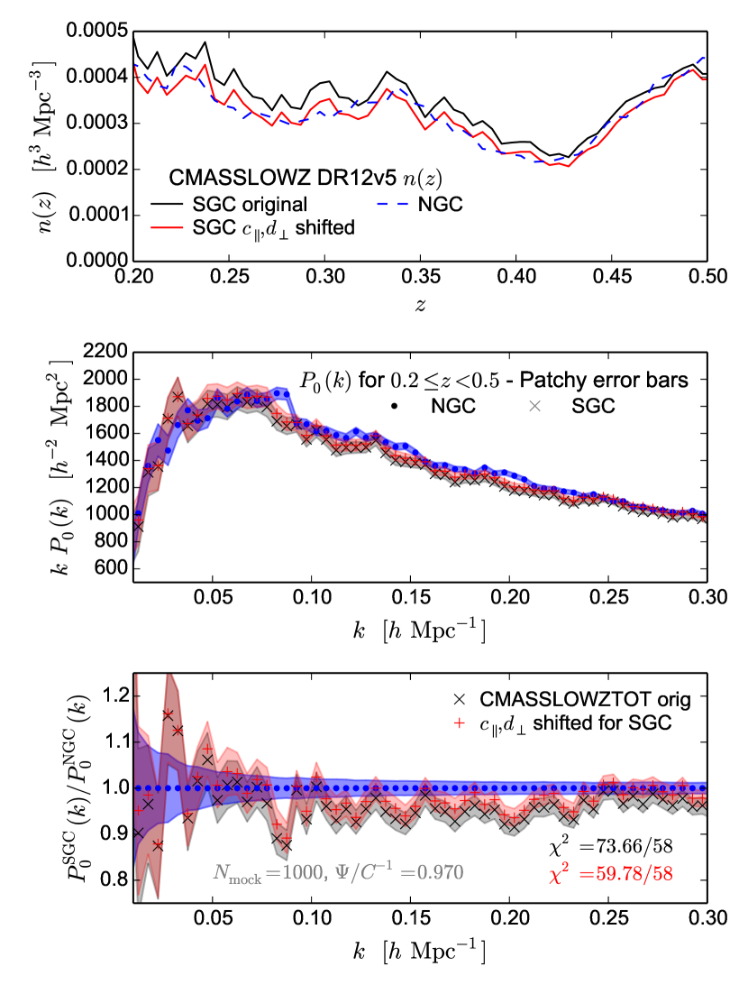
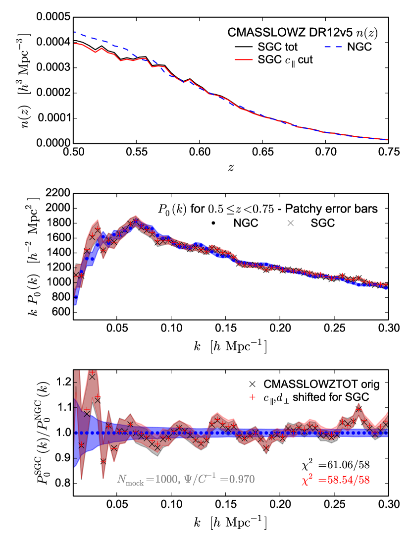
In Fig. 21, we show the power spectrum monopole for each subsample with error bars derived from the diagonal of the MD-Patchy covariance matrix (described in section 4) for the low (left-hand panels) and high (right-hand panels) redshift bins. The centre panels show the up to a wavenumber of , the lower panels show the ratio of SGC power spectrum to the NGC power spectrum. The upper panel shows the of the different subsamples, excluding the early LOWZ regions in the North. The comparison of the measured power spectrum monopole, , of the NGC and SGC subsamples of the final catalogue with the predicted NGC–SGC dispersion from the MD-Patchy mocks shows significant tension for the low redshift bin, while the differences in the high redshift bin are consistent with the sample variance of the mocks. In terms of the power spectrum monopole, the SGC clustering in the low redshift bin shows a 4 per cent amplitude mismatch.
As discussed in more detail in Ross et al. (2016), the discrepancy can be solved by taking into account the colour shifts between SDSS DR8 photometry (Aihara et al., 2011) in the North and South that have been identified by Schlafly & Finkbeiner (2011). These corrections affect the LOWZ SGC colour cut on (Reid et al., 2016, equation 9),
| (25) |
where , and the CMASS SGC colour cuts on (Reid et al., 2016, equations 13 and 14),
| (26) |
where .
The selection function and power spectrum monopole of the corrected SGC subsample are overplotted in Fig. 21. The SGC is reduced by 10 per cent at low redshifts. The power spectrum monopole of the corrected SGC sample has a larger amplitude than the original sample, but is still lower than the one of NGC for most wavenumber bins. As the window function induces a correlation between the measurement bins, only the analysis of the log likelihood , can quantify the level of consistency. We obtain the inverse covariance matrix from the inverse of the co-added NGC and SGC covariance matrices,
| (27) |
These covariance matrices of the subsamples were obtained from 1000 MD-Patchy realizations. We correct the inverse of the co-added covariance matrix for sampling noise using the correction factor as proposed in Hartlap et al. (2006), , that is given in the figure.
The analysis shows that the amplitude mismatch in is lowered to a level that is consistent with the North. The low-redshift NGC–SGC difference in the corrected sample is of the order of what can be expected ( instead of for bins) given the distribution of the mock catalogues. Further, the high redshift bin also shows slightly increased consistency ( for bins), even though it was already in good agreement in the original sample ().
These results on the shifts of and are in good agreement with those obtained in the configuration space analysis of the DR9 CMASS sample presented in Ross et al. (2012). In that work, no significant effect on the galaxy clustering was found correcting for the shifted photometry. Further tests on the DR12 combined sample in configuration space (Ross et al., 2016) show a much better degree of consistency than what is seen in Fourier space. The amplitude mismatch for the correlation function is not significant as the broad-band effect seen in Fourier space corresponds to scales smaller than those probed in the clustering analysis (). Also, the relative errors bars are larger in configuration space.
Due to the significant deviations in and between the NGC and SGC subsamples, we see this analysis as good evidence that these two subsamples probe slightly different galaxy populations for redshifts lower than .