The clustering of galaxies in the completed SDSS-III Baryon Oscillation Spectroscopic Survey: double-probe measurements from BOSS galaxy clustering & Planck data – towards an analysis without informative priors

Abstract

We develop a new methodology called double-probe analysis with the aim of minimizing informative priors in the estimation of cosmological parameters. Using our new methodology, we extract the dark-energy-model-independent cosmological constraints from the joint data sets of Baryon Oscillation Spectroscopic Survey (BOSS) galaxy sample and Planck cosmic microwave background (CMB) measurement. We measure the mean values and covariance matrix of $\{R$, $l_{a}$, $\Omega_{b}h^{2}$, $n_{s}$, $log(A_{s})$, $\Omega_{k}$, $H(z)$, $D_{A}(z)$, $f(z)\sigma_{8}(z)\}$, which give an efficient summary of Planck data and 2-point statistics from BOSS galaxy sample. The CMB shift parameters are $R=\sqrt{\Omega_{m}H_{0}^{2}}\,r(z_{*})$, and $l_{a}=\pi r(z_{*})/r_{s}(z_{*})$, where $z_{*}$ is the redshift at the last scattering surface, and $r(z_{*})$ and $r_{s}(z_{*})$ denote our comoving distance to $z_{*}$ and sound horizon at $z_{*}$ respectively; $\Omega_{b}$ is the baryon fraction at $z=0$. The advantage of this method is that we do not need to put informative priors on the cosmological parameters that galaxy clustering is not able to constrain well, i.e. $\Omega_{b}h^{2}$ and $n_{s}$.

Using our double-probe results, we obtain $\Omega_{m}=0.304\pm 0.009$, $H_{0}=68.2\pm 0.7$, and $\sigma_{8}=0.806\pm 0.014$ assuming $\Lambda$CDM; $\Omega_{k}=0.002\pm 0.003$ assuming oCDM; $w=-1.04\pm 0.06$ assuming $w$CDM; $\Omega_{k}=0.002\pm 0.003$ and $w=-1.00\pm 0.07$ assuming o$w$CDM; and $w_{0}=-0.84\pm 0.22$ and $w_{a}=-0.66\pm 0.68$ assuming $w_{0}w_{a}$CDM. The results show no tension with the flat $\Lambda$CDM cosmological paradigm. By comparing with the full-likelihood analyses with fixed dark energy models, we demonstrate that the double-probe method provides robust cosmological parameter constraints which can be conveniently used to study dark energy models.

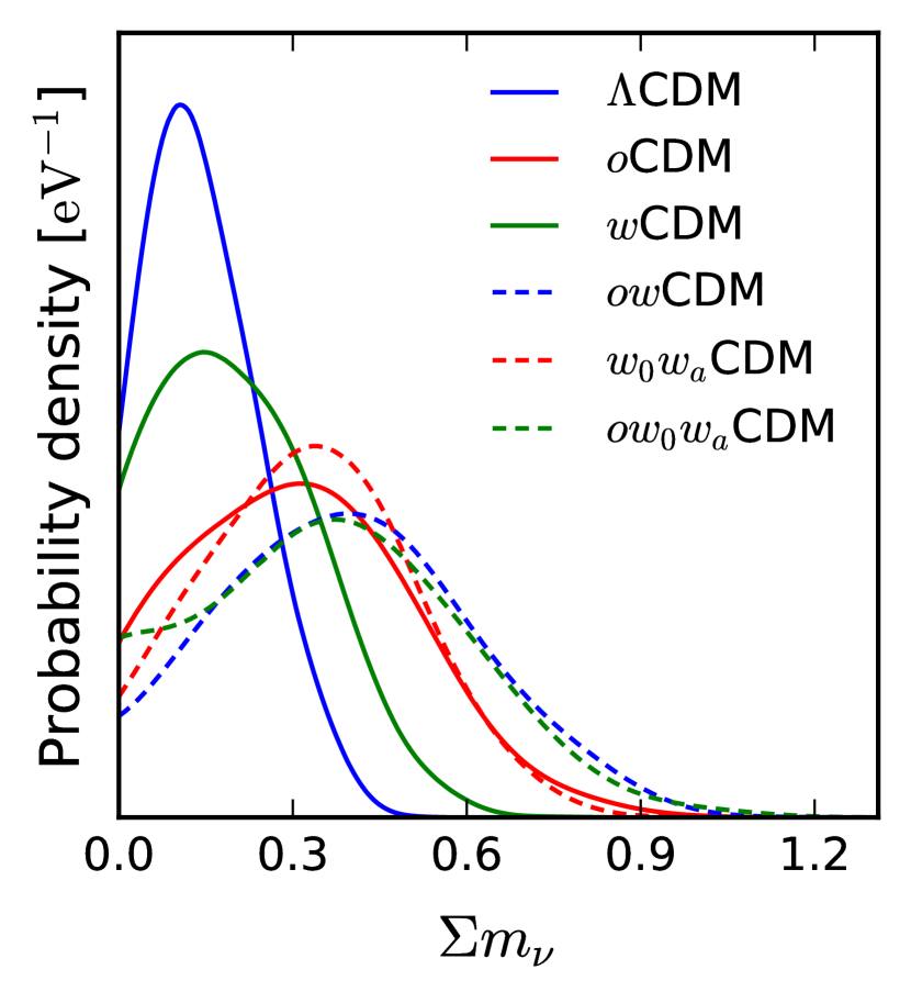
We extend our study to measure the sum of neutrino mass using different methodologies including double probe analysis (introduced in this study), the full-likelihood analysis, and single probe analysis. From the double probe analysis, we obtain $\Sigma m_{\nu}<0.10/0.22$ (68%/95%) assuming $\Lambda$CDM and $\Sigma m_{\nu}<0.26/0.52$ (68%/95%) assuming $w$CDM. This paper is part of a set that analyses the final galaxy clustering dataset from BOSS.

1 Introduction

We have entered the era of precision cosmology along with the dramatically increasing amount of sky surveys, including the cosmic microwave background (CMB; e.g., Bennett et al. 2013; Ade et al. 2014a), supernovae (SNe; Riess et al. 1998; Perlmutter et al. 1999), weak lensing (e.g., see Van Waerbeke & Mellier 2003 for a review), and large-scale structure from galaxy redshift surveys, e.g. 2dF Galaxy Redshift Survey (2dFGRS; Colless et al. 2001, 2003, Sloan Digital Sky Survey (SDSS, York et al. 2000; Abazajian et al. 2009, WiggleZ (Drinkwater et al., 2010; Parkinson et al., 2012), and the Baryon Oscillation Spectroscopic Survey (BOSS; Dawson et al. 2013; Alam et al. 2015) of the SDSS-III (Eisenstein et al., 2011). The future galaxy redshift surveys, e.g. Euclid (Laureijs et al., 2011), Dark Energy Spectroscopic Instrument (DESI; Schlegel et al. 2011), and WFIRST (Green et al., 2012), will collect data at least an order of magnitude more. It is critical to develop the methodologies which could reliably extract the cosmological information from such large amount of data.

The galaxy redshifts samples have been analysed studied in a cosmological context (see, e.g., Tegmark et al. 2004; Hutsi 2005; Padmanabhan et al. 2007; Blake et al. 2007; Percival et al. 2007; Percival et al. 2010; Reid et al. 2010; Montesano et al. 2012; Eisenstein et al. 2005; Okumura et al. 2008; Cabre & Gaztanaga 2009; Martinez et al. 2009; Sanchez et al. 2009; Kazin et al. 2010; Chuang et al. 2012; Samushia et al. 2012; Padmanabhan et al. 2012; Xu et al. 2013; Anderson et al. 2013; Manera et al. 2012; Nuza et al. 2013; Reid et al. 2012; Samushia et al. 2013; Tojeiro et al. 2012; Anderson et al. 2014b; Chuang et al. 2013a; Sanchez et al. 2013; Kazin et al. 2013; Wang 2014; Anderson et al. 2014a; Beutler et al. 2014b; Samushia et al. 2014; Chuang et al. 2013b; Sanchez et al. 2014; Ross et al. 2014; Tojeiro et al. 2014; Reid et al. 2014; Alam et al. 2015; Gil-Marín et al. 2015a, b; Cuesta et al. 2015).

Eisenstein et al. (2005) demonstrated the feasibility of measuring $\Omega_{m}h^{2}$ and an effective distance, $D_{V}(z)$ from the SDSS DR3 (Abazajian et al., 2005) LRGs, where $D_{V}(z)$ corresponds to a combination of Hubble expansion rate $H(z)$ and angular-diameter distance $D_{A}(z)$. Chuang & Wang (2012) demonstrated the feasibility of measuring $H(z)$ and $D_{A}(z)$ simultaneously using the galaxy clustering data from the two dimensional two-point correlation function of SDSS DR7 (Abazajian et al., 2009) LRGs and it has been improved later on in Chuang & Wang (2013b, a) upgrading the methodology and modelling to measure $H(z)$, $D_{A}(z)$, the normalized growth rate $f(z)\sigma_{8}(z)$, and the physical matter density $\Omega_{m}h^{2}$ from the same data. Analyses have been perform to measure $H(z)$, $D_{A}(z)$, and $f(z)\sigma_{8}(z)$ from earlier data release of SDSS BOSS galaxy sample Reid et al. (2012); Chuang et al. (2013a); Wang (2014); Anderson et al. (2014a); Beutler et al. (2014b); Chuang et al. (2013b); Samushia et al. (2014).

There are some cosmological parameters, e.g. $\Omega_{b}h^{2}$ (the physical baryon fraction) and $n_{s}$ (the scalar index of the power law primordial fluctuation), not well constrained by galaxy clustering analysis. We usually use priors adopted from CMB measurements or fix those to the best fit values obtained from CMB while doing Markov Chain Monte Carlo (MCMC) analysis. There would be some concern of missing weak degeneracies between these parameters and those measured. These could lead to incorrect constraints if models with very different predictions are tested, or double-counting when combining with CMB measurements. One might add some systematics error budget to be safe from the potential bias (e.g., see Anderson et al. (2014a)). An alternative approach is to use a very wide priors, e.g. 5 or 10 $\sigma$ flat priors from CMB, to minimize the potential systematics bias from priors (e.g., see Chuang et al. (2012); Chuang & Wang (2012)). However, the approach would obtain weaker constraints due to the wide priors. In this study, we test the ways in which LSS constraints are combined with CMB data, focussing on the information content, and the priors used when analysing LSS data. Since CMB data can be summarized with few parameters (e.g., see Wang & Mukherjee (2007)), we use the joint data set from Planck and BOSS to extract the cosmological constraints without fixing dark energy models. By combining the CMB data and the BOSS data in the upstream of the data analysis to constrain the cosmological constraints, we call our method ”double-probe analysis”. Our companion paper, Chuang et al. (2016), constrains geometric and growth information from the BOSS data alone independent of the CMB data, thereby dubbed ”single-probe”, and combines with the CMB data in the downstream of the analysis. Note that we assume there is no early time dark energy or dark energy clustering in this study. $\Omega_{b}h^{2}$ and $n_{s}$ will be well constrained by CMB so that we will obtain the cosmological constraints without concerning the problem of priors. The only input parameter which is not well constrained by our analysis is the galaxy bias on which is applied a wide flat prior. In principle, our methodology extract the cosmological constraints from the joint data set with the optimal way since we do not need to include the uncertainty introduced by the priors.

In addition to constraining dark energy model parameters, we extend our study to constrain neutrino masses. High energy physics experiments provides with the squared of mass differences between neutrino species from oscillation neutrino experiments. Latest results are $\Delta m^{2}_{21}=7.53\pm 0.18\times 10^{-5}eV^{2}$ and $\Delta m^{2}_{32}=2.44\pm 0.06\times 10^{-3}eV^{2}$ for the normal hierarchy ($m_{3}\gg m_{2}\simeq m_{1}$) and $\Delta m^{2}_{32}=2.52\pm 0.07\times 10^{-3}eV^{2}$ for the inverted mass hierarchy ($m_{3}\ll m_{2}\simeq m_{1}$) (Olive & Group 2014). Cosmology shows as a unique tool for the measurement of the sum of neutrino masses $\Sigma m_{\nu}$, since this quantity affects the expansion rate and the way structures form and evolve. $\Sigma m_{\nu}$ estimations from galaxy clustering has been widely studied theoretically (see Hu et al. 1998; Lesgourgues & Pastor 2006 for a review) and with different samples such as WiggleZ (see Riemer-Sørensen et al. 2014; Cuesta et al. 2015) or SDSS data (see Aubourg et al. 2015; Beutler et al. 2014a; Reid et al. 2010; Thomas et al. 2010; Zhao et al. 2013). At late times, massive neutrinos can damp the formation of cosmic structure on small scales due to the free-streaming effect (Dolgov, 2002). Existing in the form of radiation in the early Universe, neutrinos shift the epoch of the matter-radiation equality thus changing the shape of the cosmic microwave background (CMB) angular power spectrum. They affect CMB via the so called Early Integrated Sachs Wolfe Effect and they influence gravitational lensing measurements (e.g., see Lesgourgues et al. 2006). Recent publications have attempted to constrain $\Sigma m_{\nu}$ , imposing upper limits (Seljak et al., 2006; Hinshaw et al., 2009; Dunkley et al., 2009; Reid et al., 2010; Komatsu et al., 2011; Saito et al., 2011; Tereno et al., 2009; Gong et al., 2008; Ichiki et al., 2009; Li et al., 2009; de Putter et al., 2012; Xia et al., 2012; Sanchez et al., 2012; Giusarma et al., 2013) and some hints of lower limits using cluster abundance results (Ade et al., 2014b; Battye & Moss, 2014; Wyman et al., 2014; Burenin, 2013; Rozo et al., 2013). We measure the sum of neutrino mass using different methodologies including double probe analysis (introduced in this study), the full-likelihood analysis, and single probe analysis (Chuang et al. 2016; companion paper).

This paper is organized as follows. In Section 2, we introduce the Planck data, the SDSS-III/BOSS DR12 galaxy sample and mock catalogues used in our study. In Section 3, we describe the details of the methodology that constrains cosmological parameters from our joint CMB and galaxy clustering analysis. In Section 4, we present our double-probe cosmological measurements. In Section 5, we demonstrate how to derive cosmological constraints from our measurements with some given dark energy model. In Section 6, opposite to the manner of dark energy model independent method, we present the results from the full-likelihood analysis with fixing dark energy models. In Section 7, we measure the sum of neutrino mass with different methodologies. We summarize and conclude in Section 8.

2 Data sets & mocks

2.1 The SDSS-III/BOSS Galaxy Catalogues

The Sloan Digital Sky Survey (SDSS; Fukugita et al. 1996; Gunn et al. 1998; York et al. 2000; Smee et al. 2013) mapped over one quarter of the sky using the dedicated 2.5 m Sloan Telescope (Gunn et al., 2006). The Baryon Oscillation Sky Survey (BOSS, Eisenstein et al. 2011; Bolton et al. 2012; Dawson et al. 2013) is part of the SDSS-III survey. It is collecting the spectra and redshifts for 1.5 million galaxies, 160,000 quasars and 100,000 ancillary targets. The Data Release 12 (Alam et al., 2015) has been made publicly available. We use galaxies from the SDSS-III BOSS DR12 CMASS catalogue in the redshift range $0.43<z<0.75$ and LOWZ catalogue in the range $0.15<z<0.43$. CMASS samples are selected with an approximately constant stellar mass threshold (Eisenstein et al., 2011); LOWZ sample consists of red galaxies at $z<0.4$ from the SDSS DR8 (Aihara et al., 2011) image data. We are using 800853 CMASS galaxies and 361775 LOWZ galaxies. The effective redshifts of the sample are $z=0.59$ and $z=0.32$ respectively. The details of generating this sample are described in Reid et al. (2016).

2.2 The Planck Data

Planck (Tauber et al., 2010; Planck Collaboration I, 2011) is the third generation space mission, following COBE and WMAP, to measure the anisotropy of the CMB. It observed the sky in nine frequency bands covering the range 30–857 GHz with high sensitivity and angular resolutions from 31’ to 5’. The Low Frequency Instrument (LFI; Bersanelli et al., 2010; Mennella et al., 2011) covers the bands centred at 30, 44, and 70 GHz using pseudo-correlation radiometers detectors, while the High Frequency Instrument (HFI; Planck HFI Core Team, 2011) covers the 100, 143, 217, 353, 545, and 857 GHz bands with bolometers. Polarisation is measured in all but the highest two bands (Leahy et al., 2010; Rosset et al., 2010). In this paper, we used the 2015 Planck release (Planck Collaboration I, 2015), which included the full mission maps and associated data products.

2.3 The Mock Galaxy Catalogues

We use 2000 BOSS DR12 MultiDark-PATCHY (MD-PATCHY) mock galaxy catalogues (Kitaura et al., 2015b) for validating our methodology and estimating the covariance matrix in this study. These mock catalogues were constructed using a similar procedure described in Rodríguez-Torres et al. 2015 where they constructed the BOSS DR12 lightcone mock catalogues using the MultiDark $N$-body simulations. However, instead of using $N$-body simulations, the 2000 MD-PATCHY mocks catalogues were constructed using the PATCHY approximate simulations. These mocks are produced using ten boxes at different redshifts that are created with the PATCHY-code (Kitaura et al., 2014). The PATCHY-code is composed of two parts: 1) computing approximate dark matter density field; and 2) populating galaxies from dark matter density field with the biasing model. The dark matter density field is estimated using Augmented Lagrangian Perturbation Theory (ALPT; Kitaura & Hess (2013)) which combines the second order perturbation theory (2LPT; e.g. see Buchert (1994); Bouchet et al. (1995); Catelan (1995)) and spherical collapse approximation (see Bernardeau (1994); Mohayaee et al. (2006); Neyrinck (2013)). The biasing model includes deterministic bias and stochastic bias (see Kitaura et al. (2014); Kitaura et al. (2015) for details). The velocity field is constructed based on the displacement field of dark matter particles. The modeling of finger-of-god has also been taken into account statistically. The mocks match the clustering of the galaxy catalogues for each redshift bin (see Kitaura et al. (2015b) for details) and have been used in recent galaxy clustering studies (Cuesta et al., 2015; Gil-Marín et al., 2015a, b; Rodríguez-Torres et al., 2015; Slepian et al., 2015) and void clustering studies (Kitaura et al., 2015a; Liang et al., 2015). They are also used in Alam et al. (2016) (BOSS collaboration paper for final data release) and its companion papers (this paper and Ross et al. (2016); Vargas-Magana et al. (2016); Beutler et al. (2016a); Satpathy et al. (2016); Beutler et al. (2016b); Sanchez et al. (2016a); Grieb et al. (2016); Sanchez et al. (2016b); Chuang et al. (2016); Slepian et al. (2016a, b); Salazar-Albornoz et al. (2016); Zhao et al. (2016); Wang et al. (2016)

3 Methodology

We develop a new methodology to extract the cosmological constraints from the joint data set of the Planck CMB data and BOSS galaxy clustering measurements fitting the LSS data with parameter combinations defining the key cosmological dependencies, while including CMB constraints to simultaneously constrain other parameters. This means that we can define constraints that can subsequently be used to constrain a wide-range of Dark Energy models. Similar approaches have been applied to these data separately. Our work is the first to investigate how in detail this joint analysis should be performed.

3.1 Likelihood from BOSS galaxy clustering

In this section, we describe the steps to compute the likelihood from the BOSS galaxy clustering.

3.1.1 Measure Multipoles of the Two-Point Correlation Function

We convert the measured redshifts of the BOSS CMASS and LOWZ galaxies to comoving distances by assuming a fiducial model, i.e., flat $\Lambda$CDM with $\Omega_{m}=0.307115$ and $h=0.6777$ which is the same model adopted for constructing the mock catalogues (see Kitaura et al. (2015b) ). To compute the two-dimensional two-point correlation function, we use the two-point correlation function estimator given by Landy & Szalay (1993):

$$\xi(s,\mu)=\frac{DD(s,\mu)-2DR(s,\mu)+RR(s,\mu)}{RR(s,\mu)},$$ (1)

where $s$ is the separation of a pair of objects and $\mu$ is the cosine of the angle between the directions between the line of sight (LOS) and the line connecting the pair the objects. DD, DR, and RR represent the normalized data-data, data-random, and random-random pair counts, respectively, for a given distance range. The LOS is defined as the direction from the observer to the centre of a galaxy pair. Our bin size is $\Delta s=1\,h^{-1}$Mpc and $\Delta\mu=0.01$. The Landy and Szalay estimator has minimal variance for a Poisson process. Random data are generated with the same radial and angular selection functions as the real data. One can reduce the shot noise due to random data by increasing the amount of random data. The number of random data we use is about 50 times that of the real data. While calculating the pair counts, we assign to each data point a radial weight of $1/[1+n(z)\cdot P_{w}]$, where $n(z)$ is the radial number density and $P_{w}=1\cdot 10^{4}$ $h^{-3}$Mpc³ (see Feldman et al. 1994).

The traditional multipoles of the two-point correlation function, in redshift space, are defined by

$$\xi_{l}(s) \equiv \frac{2l+1}{2}\int_{-1}^{1}{\rm d}\mu\,\xi(s,\mu)P_{l}(\mu),$$

where $P_{l}(\mu)$ is the Legendre Polynomial ($l=$0 and 2 here). We integrate over a spherical shell with radius $s$, while actual measurements of $\xi(s,\mu)$ are done in discrete bins. To compare the measured $\xi(s,\mu)$ and our theoretical model, the last integral in Eq.(3.1.1) should be converted into a sum,

$$\hat{\xi}_{l}(s)\equiv\frac{\displaystyle\sum_{s-\frac{\Delta s}{2}<s^{\prime}<s+\frac{\Delta s}{2}}\displaystyle\sum_{0\leq\mu\leq 1}(2l+1)\xi(s^{\prime},\mu)P_{l}(\mu)}{\mbox{Number of bins used in the numerator}},$$ (2)

where $\Delta s=5$ $h^{-1}$Mpc in this work.

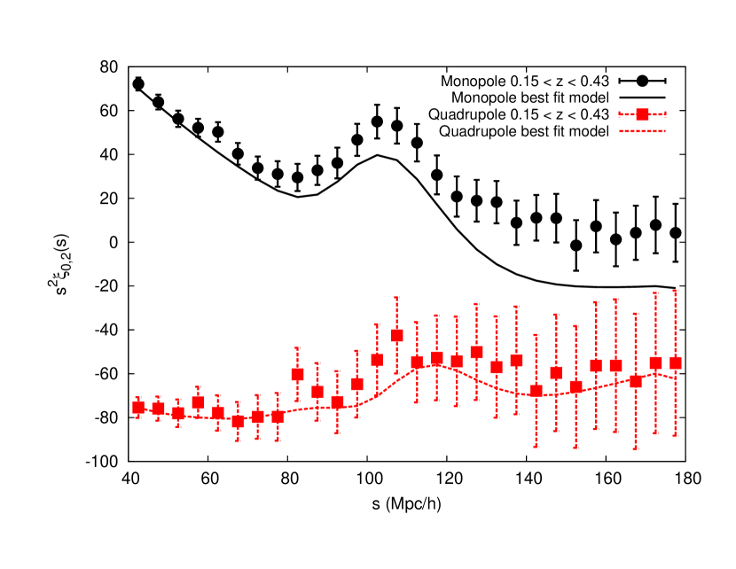
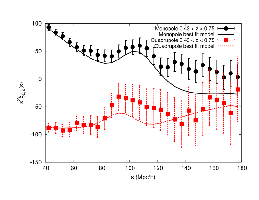
Fig.1 shows the monopole ($\hat{\xi}_{0}$) and quadrupole ($\hat{\xi}_{2}$) measured from the BOSS CMASS and LOWZ galaxy sample compared with the best fit theoretical models.

We are using the scale range $s=40-180\,h^{-1}$Mpc and the bin size is 5 $h^{-1}$Mpc. The data points from the multipoles in the scale range considered are combined to form a vector, $X$, i.e.,

$${\bf X}=\{\hat{\xi}_{0}^{(1)},\hat{\xi}_{0}^{(2)},...,\hat{\xi}_{0}^{(N)};\hat{\xi}_{2}^{(1)},\hat{\xi}_{2}^{(2)},...,\hat{\xi}_{2}^{(N)};...\},$$ (3)

where $N$ is the number of data points in each measured multipole; here $N=28$. The length of the data vector ${\bf X}$ depends on the number of multipoles used.

Figure 1: Left panel: measurement of monopole and quadrupole of the correlation function from the BOSS DR12 LOWZ galaxy sample within $0.15<z<0.43$ compared to the best fited theoretical models (solid lines). Right panel: measurement of effective monopole and quadrupole of the correlation function from the BOSS DR12 CMASS galaxy sample within $0.43<z<0.75$ compared to the best fitted theoretical models (solid lines). The error bars are the square roots of the diagonal elements of the covariance matrix. In this study, our fitting scale ranges are $40h^{-1}$Mpc $<s<180h^{-1}$Mpc; the bin size is $5h^{-1}$Mpc.

3.1.2 Theoretical Two-Point Correlation Function

Following Chuang et al. (2016), companion paper, we use two models to compute the likelihood of the galaxy clustering measurements. One is a fast model which is used to narrow down the parameters space scanned; the other is a slower model which is used to calibrate the results from the fast model.

Fast model: The fast model we use is the two-dimensional dewiggle model explained in Chuang et al. (2016), companion paper. The theoretical model can be constructed by first and higher order perturbation theory. We first adopt the cold dark matter model and the simplest inflation model (adiabatic initial condition). Computing the linear matter power spectra, $P_{lin}(k)$, by using CAMB (Code for Anisotropies in the Microwave Background, Lewis et al. 2000) we can decomposed it into two parts:

$$P_{lin}(k)=P_{nw}(k)+P_{BAO}^{lin}(k),$$ (4)

where $P_{nw}(k)$ is the “no-wiggle” power spectrum calculated using Eq.(29) from Eisenstein & Hu (1998) and $P_{BAO}^{lin}(k)$ is the “wiggled” part defined by previous Eq. (4). Nonlinear damping effect of the “wiggled” part, in redshift space, is approximated following Eisenstein et al. (2007) by

$$P_{BAO}^{nl}(k,\mu_{k})=P_{BAO}^{lin}(k)\cdot\exp\left(-\frac{k^{2}}{2k_{\star}^{2}}[1+\mu_{k}^{2}(2f+f^{2})]\right),$$ (5)

where $\mu_{k}$ is the cosine of the angle between ${\bf k}$ and the LOS, $f$ is the growth rate, and $k_{\star}$ is computed following Crocce & Scoccimarro (2006) and Matsubara (2008) by

$$k_{\star}=\left[\frac{1}{3\pi^{2}}\int P_{lin}(k)dk\right]^{-1/2}.$$ (6)

Thus dewiggled power spectrum is

$$P_{dw}(k,\mu_{k})=P_{nw}(k)+P_{BAO}^{nl}(k,\mu_{k}).$$ (7)

We include the linear redshift distortion as follows (reference (Kaiser, 1987)),

$$P_{g}^{s}(k,\mu_{k}) = b^{2}(1+\beta\mu_{k}^{2})^{2}P_{dw}(k,\mu_{k}),$$ (8)

where $b$ is the linear galaxy bias and $\beta$ is the linear redshift distortion parameter.

To compute the theoretical two-point correlation function, $\xi(s,\mu)$, we Fourier transform the non-linear power spectrum $P_{g}^{s}(k,\mu_{k})$ by using Legendre polynomial expansions and one-dimensional integral convolutions as introduced in Chuang & Wang (2013a).

We times calibration functions to the fast model by

$$\xi_{0}^{cal}(s)=(1-e^{-\frac{s}{s_{1}}}+e^{-\left(\frac{s}{s_{2}}\right)^{2}})\xi_{0}(s),$$ (9)

$$\xi_{2}^{cal}(s)=(1-e^{-\frac{s}{s_{3}}}+e^{-\left(\frac{s}{s_{4}}\right)^{2}})\xi_{2}(s),$$ (10)

so that it mimics the slow model presented bellow. We find the calibration parameters, $s_{1}=12$, $s_{2}=14$, $s_{3}=20$, and $s_{4}=27$, by comparing the fast and slow models by visual inspection. It is not critical to find the best form of calibration function and its parameters as the model will be callibrated later when performing importance sampling with slow model.

Slow model: The slower but accurate model we use is ”Gaussian streaming model” described in Reid & White (2011). The model assumes that the pairwise velocity probability distribution function is Gaussian and can be used to relate real space clustering and pairwise velocity statistics of halos to their clustering in redshift space by

$$1+\xi^{s}_{\rm g}(r_{\sigma},r_{\pi})=$$

$$\int\left[1+\xi^{r}_{\rm g}(r)\right]e^{-[r_{\pi}-y-\mu v_{12}(r)]^{2}/2\sigma_{12}^{2}(r,\mu)}\frac{dy}{\sqrt{2\pi\sigma^{2}_{12}(r,\mu)}},$$ (11)

where $r_{\sigma}$ and $r_{\pi}$ are the redshift space transverse and LOS distances between two objects with respect to the observer, $y$ is the real space LOS pair separation, $\mu=y/r$, $\xi_{\rm g}^{\rm r}$ is the real space galaxy correlation function, $v_{12}(r)$ is the average infall velocity of galaxies separated by real-space distance $r$, and $\sigma_{12}^{2}(r,\mu)$ is the rms dispersion of the pairwise velocity between two galaxies separated with transverse (LOS) real space separation $r_{\sigma}$ ($y$). $\xi_{\rm g}^{\rm r}(r)$, $v_{12}(r)$ and $\sigma_{12}^{2}(r,\mu)$ are computed in the framework of Lagrangian ($\xi^{\rm r}$) and standard perturbation theories ($v_{12}$, $\sigma_{12}^{2}$).

For large scales, only one nuisance parameter is necessary to describe the clustering of a sample of halos or galaxies in this model: $b_{1L}=b-1$, the first-order Lagrangian host halo bias in real space. In this study, we consider relative large scales (i.e. $40<s<180h^{-1}$Mpc), so that we do not include $\sigma^{2}_{\rm FoG}$, to model a velocity dispersion accounting for small-scale motions of halos and galaxies. Further details of the model, its numerical implementation, and its accuracy can be found in Reid & White (2011).

3.1.3 Covariance Matrix

We use the 2000 mock catalogues created by Kitaura et al. 2015b for the BOSS DR12 CMASS and LOWZ galaxy sample to estimate the covariance matrix of the observed correlation function. We calculate the multipoles of the correlation functions of the mock catalogues and construct the covariance matrix as

$$C_{ij}=\frac{1}{(N-1)(1-D)}\sum^{N}_{k=1}(\bar{X}_{i}-X_{i}^{k})(\bar{X}_{j}-X_{j}^{k}),$$ (12)

where

$$D=\frac{N_{b}+1}{N-1},$$ (13)

$N$ is the number of the mock catalogues, $N_{b}$ is the number of data bins, $\bar{X}_{m}$ is the mean of the $m^{th}$ element of the vector from the mock catalogue multipoles, and $X_{m}^{k}$ is the value in the $m^{th}$ elements of the vector from the $k^{th}$ mock catalogue multipoles. The data vector ${\bf X}$ is defined by Eq.(3). We also include the correction, $D$, introduced by Hartlap et al. (2007).

3.1.4 Compute Likelihood from Galaxy Clustering

The likelihood is taken to be proportional to $\exp(-\chi^{2}/2)$ (B.P., 1992), with $\chi^{2}$ given by

$$\chi^{2}\equiv\sum_{i,j=1}^{N_{X}}\left[X_{th,i}-X_{obs,i}\right]C_{ij}^{-1}\left[X_{th,j}-X_{obs,j}\right]$$ (14)

where $N_{X}$ is the length of the vector used, $X_{th}$ is the vector from the theoretical model, and $X_{obs}$ is the vector from the observed data.

As explained in Chuang & Wang (2012), instead of recalculating the observed correlation function while computing for different models, we rescale the theoretical correlation function to avoid rendering the $\chi^{2}$ values arbitrary. This approach can be considered as an application of Alcock-Paczynski effect (Alcock & Paczynski, 1979). The rescaled theoretical correlation function is computed by

$$T^{-1}(\xi_{th}(\sigma,\pi))=\xi_{th}\left(\frac{D_{A}(z)}{D_{A}^{fid}(z)}\sigma,\frac{H^{fid}(z)}{H(z)}\pi\right),$$ (15)

where $\xi_{th}$ is the theoretical model computed in Sec. 3.1.2. Here, $D_{A}(z)$ and $H(z)$ would be the input parameters and $D_{A}^{fid}(z)$ and $H^{fid}(z)$ are $\{990.20$Mpc, $80.16\,{\rm km}\,{\rm s}^{-1}\,{\rm Mpc}^{-1}\}$ at $z=0.32$ (LOWZ) and $\{1409.26$Mpc, $94.09\,{\rm km}\,{\rm s}^{-1}\,{\rm Mpc}^{-1}\}$ at $z=0.59$ (CMASS). Then, $\chi^{2}$ can be rewritten as

$$\chi^{2} \equiv \sum_{i,j=1}^{N_{X}}\left\{T^{-1}X_{th,i}-X^{fid}_{obs,i}\right\}C_{fid,ij}^{-1}\cdot$$ (16)

$$\cdot\left\{T^{-1}X_{th,j}-X_{obs,j}^{fid}\right\};$$

where $T^{-1}X_{th}$ is the vector computed by eq. (2) from the rescaled theoretical correlation function, eq. (15). $X^{fid}_{obs}$ is the vector from observed data measured with the fiducial model (see Chuang & Wang 2012 for more details regarding the rescaling method).

3.2 Likelihood from Planck CMB data

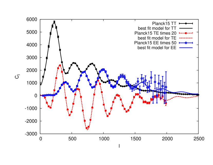
Our CMB data set consists of the Planck 2015 measurements (Planck Collaboration I, 2015; Planck Collaboration XIII, 2015). The reference likelihood code (Planck Collaboration XI, 2015) was downloaded from the Planck Legacy Archive. Here we combine the Plik baseline likelihood for high multipoles ($30\leq\ell\leq 2500$) using the TT, TE and EE power spectra, and the Planck low-$\ell$ multipole likelihood in the range $2\leq\ell\leq 29$ (hereafter lowTEB). We also include the new Planck 2015 lensing likelihood (Planck Collaboration XV, 2015), constructed from the measurements of the power spectrum of the lensing potential (hereafter referred as ”lensing”). We using the Planck lensing likelihood, the $A_{\rm lens}$ parameter is always set to 1 (Planck Collaboration XIII, 2015).

Figure 2: Angular power spectrum of temperature and polarization measurement from Planck data and their best fits from our double probe analysis.

3.3 Markov Chain Monte-Carlo Likelihood Analysis

3.3.1 basic procedure

We perform Markov Chain Monte Carlo (MCMC) likelihood analyses using CosmoMC (Lewis & Bridle, 2002; Lewis, 2013). The fiducial parameter space that we explore spans the parameter set of $\{\Omega_{c}h^{2}$, $\Omega_{b}h^{2}$, $n_{s}$, $log(A_{s})$, $\theta$, $\tau$, $\Omega_{k}$, $w$,$H(z)$, $D_{A}(z)$, $\beta(z)$, $b\sigma_{8}(z)$, $b(z)\}$. The quantities $\Omega_{c}$ and $\Omega_{b}$ are the cold dark matter and baryon density fractions, $n_{s}$ is the power-law index of the primordial matter power spectrum, $\Omega_{k}$ is the curvature density fraction, $w$ is the equation state of dark energy, $h$ is the dimensionless Hubble constant ($H_{0}=100h$ km s^-1Mpc^-1), and $\sigma_{8}(z)$ is the normalization of the power spectrum. Note that, with the joint data set (Planck + BOSS), the only parameter which is not well constrained is $b(z)$. We apply a flat prior of $(1,3)$ on it. The linear redshift distortion parameter can be expressed as $\beta(z)=f(z)/b$. Thus, one can derive $f(z)\sigma_{8}(z)$ from the measured $\beta(z)$ and $b\sigma_{8}(z)$.

3.3.2 Generate Markov chains with fast model

We first use the fast model (2D dewiggle model) to compute the likelihood, $\mathcal{L}_{fast}$ and generate the Markov chains. The Monte Carlo analysis will go through many random steps keeping or throwing the computed points parameter space according to the Markov likelihood algorithm. Eventually, it will provide the chains of parameter points with high likelihood describing the constraints to our model.

3.3.3 Calibrate the likelihood using slow model

Once we have the fast model generated chains, we modify the weight of each point by

$$\mathcal{W}_{new}=\mathcal{W}_{old}\frac{\mathcal{L}_{slow}}{\mathcal{L}_{fast}},$$ (17)

where $\mathcal{L}_{slow}$ and $\mathcal{L}_{fast}$ are the likelihood for given point of input parameters in the chains. We save time by computing only the ”important” points without computing the likelihood of the ones which will not be included in the first place. The methodology is know as ”Importance sampling”. However, the typical Importance sampling method is to add likelihood of some additional data set to the given chains, but in this study, we replace the likelihood of a data set.

4 Double Probe results

The 2-point statistic of galaxy clustering can be summarized by $\{\Omega_{m}h^{2}$, $H(z)$, $D_{A}(z)$, $f(z)\sigma_{8}(z)\}$ (e.g. Chuang & Wang (2013a)). In some studies, $\Omega_{m}h^{2}$ was not included since a strong prior had been applied. Instead of using $H(z)$ and $D_{A}(z)$, one uses the derived parameters $H(z)r_{s}/r_{s,fid}$ and $D_{A}(z)r_{s,fid}/r_{s}$ to summarize the cosmological information since these two quantities are basically uncorrelated to $\Omega_{m}h^{2}$, where $r_{s}$ is the sound horizon at the redshift of the drag epoch and $r_{s,fid}$ is the $r_{s}$ of the fiducial cosmology. In this study, $\Omega_{m}h^{2}$ is well constrained by the joint data set but we still use $H(z)r_{s}/r_{s,fid}$ and $D_{A}(z)r_{s,fid}/r_{s}$ because they have tighter constraints.

Wang & Mukherjee (2007) showed that CMB shift parameters $(l_{a},R)$, together with $\Omega_{b}h^{2}$, provide an efficient and intuitive summary of CMB data as far as dark energy constraints are concerned. It is equivalent to replace $\Omega_{b}h^{2}$ with $z_{*}$, the redshift to the photon-decoupling surface (Wang, 2009). The CMB shift parameters are defined as (Wang & Mukherjee, 2007):

$$R\equiv\sqrt{\Omega_{m}H_{0}^{2}}\,r(z_{*}),$$ (18)

$$l_{a}\equiv\pi r(z_{*})/r_{s}(z_{*}),$$ (19)

and $z_{\star}$ is the redshift to the photon-decoupling surface given by CAMB (Lewis et al., 2000)

The angular comoving distance to an object at redshift $z$ is given by:

$$r(z)=cH_{0}^{-1}\,|\Omega_{k}|^{-1/2}{\rm sinn}[|\Omega_{k}|^{1/2}\,\Gamma(z)],$$ (20)

which has simple relation with the angular diameter distance $D_{A}(z)=r(z)/(1+z)$.

In additional to the shift parameters, we include also the scalar index and amplitude of the power law primordial fluctuation $n_{s}$ and $A_{s}$ to summarize the CMB information.

From the measured parameters $\{\Omega_{c}h^{2}$, $\Omega_{b}h^{2}$, $n_{s}$, $log(A_{s})$, $\theta$, $\tau$, $\Omega_{k}$, $w$,$H(z)$, $D_{A}(z)$, $\beta(z)$, $b\sigma_{8}(z)$, $b(z)\}$, we derive the parameters $\{R$, $l_{a}$, $\Omega_{b}h^{2}$, $n_{s}$, $log(10^{10}A_{s})$, $\Omega_{k}$, $H(z)r_{s}/r_{s,fid}$, $D_{A}(z)r_{s,fid}/r_{s}$, $f(z)\sigma_{8}(z)\}$ to summarize the joint data set of Planck and BOSS galaxy sample. Table  1 and 2 show the measured values and their normalized covariance. A normalized covariance matrix is defined by

$$N_{ij}=\frac{C_{ij}}{\sqrt{C_{ii}C_{jj}}},$$ (21)

where $C_{ij}$ is the covariance matrix.

To conveniently compare with other measurements using CMASS sample within $0.43<z<0.7$ (we are using $0.43<z<0.75$), we extrapolated our measurements at $z=0.57$: $H(0.57)r_{s}/r_{s,fid}=96.7\pm 3.1\,{\rm km}\,{\rm s}^{-1}\,{\rm Mpc}^{-1}$ and $D_{A}(0.57)r_{s,fid}/r_{s}=1405\pm 25$Mpc (see Table 9 of Alam et al. 2016).

$f\sigma_{8}(0.59)$	$0.510\pm 0.047$
$H(0.59)r_{s}/r_{s,fid}$	$97.9\pm 3.1$
$D_{A}(0.59)r_{s,fid}/r_{s}$	$1422\pm 25$
$f\sigma_{8}(0.32)$	$0.431\pm 0.063$
$H(0.32)r_{s}/r_{s,fid}$	$79.1\pm 3.3$
$D_{A}(0.32)r_{s,fid}/r_{s}$	$956\pm 27$
$R$	$1.7430\pm 0.0080$
$l_{a}$	$301.70\pm 0.15$
$\Omega_{b}h^{2}$	$0.02233\pm 0.00025$
$n_{s}$	$0.9690\pm 0.0066$
${\rm{ln}}(10^{10}A_{s})$	$3.040\pm 0.036$
$\Omega_{k}$	$-0.003\pm 0.006$

Table 1: Fiducial result of the double-probe approach. The units of $H(z)$ and $D_{A}(z)$ are $\,{\rm km}\,{\rm s}^{-1}\,{\rm Mpc}^{-1}$ and Mpc.

	R	la	$\Omega_{b}h^{2}$	$n_{s}$	${\rm{ln}}(10^{10}A_{s})$	$f\sigma_{8}(0.59)$	$\frac{H(0.59)}{r_{s,fid}/r_{s}}$	$\frac{D_{A}(0.59)}{r_{s}/r_{s,fid}}$	$f\sigma_{8}(0.32)$	$\frac{H(0.32)}{r_{s,fid}/r_{s}}$	$\frac{D_{A}(0.32)}{r_{s}/r_{s,fid}}$	$\Omega_{k}$
R	1.0000	0.6534	-0.7271	-0.8787	-0.0352	-0.0620	-0.1675	-0.0059	-0.0237	-0.0271	0.0027	0.6349
la	0.6534	1.0000	-0.5212	-0.5770	-0.0651	-0.1067	-0.1957	0.0017	0.0073	0.0174	-0.0211	0.4329
$\Omega_{b}h^{2}$	-0.7271	-0.5212	1.0000	0.6633	0.1175	0.0525	0.0822	0.0333	0.1373	0.0566	0.0321	-0.4070
$n_{s}$	-0.8787	-0.5770	0.6633	1.0000	0.0808	0.0381	0.1648	-0.0003	0.0285	0.0510	0.0303	-0.5547
${\rm{ln}}(10^{10}A_{s})$	-0.0352	-0.0651	0.1175	0.0808	1.0000	0.0034	0.0391	0.0175	-0.0066	0.0020	0.0516	0.5915
$f\sigma_{8}(0.59)$	-0.0620	-0.1067	0.0525	0.0381	0.0034	1.0000	0.7153	0.6172	0.1531	0.1535	-0.0333	0.0252
$H(0.59)r_{s}/r_{s,fid}$	-0.1675	-0.1957	0.0822	0.1648	0.0391	0.7153	1.0000	0.4168	0.0447	0.0968	-0.0388	-0.0959
$D_{A}(0.59)r_{s,fid}/r_{s}$	-0.0059	0.0017	0.0333	-0.0003	0.0175	0.6172	0.4168	1.0000	0.0209	-0.0319	-0.0839	0.0038
$f\sigma_{8}(0.32)$	-0.0237	0.0073	0.1373	0.0285	-0.0066	0.1531	0.0447	0.0209	1.0000	0.6581	0.5250	0.1142
$H(0.32)r_{s}/r_{s,fid}$	-0.0271	0.0174	0.0566	0.0510	0.0020	0.1535	0.0968	-0.0319	0.6581	1.0000	0.3168	0.1165
$D_{A}(0.32)r_{s,fid}/r_{s}$	0.0027	-0.0211	0.0321	0.0303	0.0516	-0.0333	-0.0388	-0.0839	0.5250	0.3168	1.0000	0.0835
$\Omega_{k}$	0.6349	0.4329	-0.4070	-0.5547	0.5915	0.0252	-0.0959	0.0038	0.1142	0.1165	0.0835	1.0000

Table 2: Normalized covariance matrix of the fiducial result from the double-probe approach.

5 constrain parameters of given dark energy models with double-probe results

In this section, we describe the steps to combine our results with other data sets assuming some dark energy models. For a given model and cosmological parameters, one can compute $\{R$, $l_{a}$, $\Omega_{b}h^{2}$, $n_{s}$, $log(10^{1}0A_{s})$, $\Omega_{k}$, $H(z)r_{s}/r_{s,fid}$, $D_{A}(z)r_{s,fid}/r_{s}$, $f(z)\sigma_{8}(z)\}$. one can take the covariance matrices, $M_{ij,\textrm{CMB+galaxy}}$, of these 12 parameters (galaxy sample are divided in two redshift bins). Then, $\chi^{2}_{\textrm{CMB+galaxy}}$ can be computed by

$$\chi^{2}_{\textrm{CMB+galaxy}}=\Delta_{\textrm{CMB+galaxy}}M_{ij,\textrm{CMB+galaxy}}^{-1}\Delta_{\textrm{CMB+galaxy}},$$ (22)

where

$$\Delta_{\textrm{CMB+galaxy}}=\left(\begin{array}[]{c}f\sigma_{8}(0.59)-0.510\\ H(0.59)r_{s}/r_{s,fid}-97.9\\ D_{A}(0.59)r_{s,fid}/r_{s}-1422\\ f\sigma_{8}(0.32)-0.431\\ H(0.32)r_{s}/r_{s,fid}-79.1\\ D_{A}(0.32)r_{s,fid}/r_{s}-956\\ R-1.7430\\ l_{a}-301.70\\ \Omega_{b}h^{2}-0.02233\\ n_{s}-0.9690\\ {\rm{ln}}(10^{10}A_{s})-3.040\\ \Omega_{k}-0.003\\ \end{array}\right),$$ (23)

where the angular diameter distance $D_{A}(z)$ is given by:

$$D_{A}(z)=(1+z)cH_{0}^{-1}\,|\Omega_{k}|^{-1/2}{\rm sinn}[|\Omega_{k}|^{1/2}\,\Gamma(z)],$$ (24)

$$\mbox{where }\Gamma(z)=\int_{0}^{z}\frac{dz^{\prime}}{E(z^{\prime})},\mbox{ and }E(z)=H(z)/H_{0},$$

and ${\rm sinn}(x)=\sin(x)$, $x$, $\sinh(x)$ for $\Omega_{k}<0$, $\Omega_{k}=0$, and $\Omega_{k}>0$ respectively; and the expansion rate the universe $H(z)$ is given by

$$H(z)=$$

$$H_{0}\sqrt{\Omega_{m}(1+z)^{3}+\Omega_{r}(1+z)^{4}+\Omega_{k}(1+z)^{2}+\Omega_{X}X(z)},$$ (25)

where $\Omega_{m}+\Omega_{r}+\Omega_{k}+\Omega_{X}=1$, and the dark energy density function $X(z)$ is defined as

$$X(z)\equiv\frac{\rho_{X}(z)}{\rho_{X}(0)}.$$ (26)

$f$ is defined in relation to the linear growth factor $D(\tau)$ in the usual way as

$$f=\frac{d\ln D(\tau)}{d\ln a}=\frac{1}{\mathcal{H}}\frac{d\ln D(\tau)}{d\tau},$$ (27)

where $D$ is the growing solution to the second order differential equation writen in comoving coordinates

$$\frac{d^{2}D(\tau)}{d\tau^{2}}+\mathcal{H}\frac{dD(\tau)}{d\tau}=\frac{3}{2}\Omega_{m}(\tau)\mathcal{H}^{2}(\tau)D(\tau).$$ (28)

We will be writing $\sigma(z,R)$ as:

$$\sigma^{2}(z,R)=\frac{1}{(2\pi)^{3}}\int d^{3}kW^{2}(kR)P(k,z)$$ (29)

with

$$W(kR)=\frac{3}{(kR)^{3}}[\sin(kR)-kR\cos(kR)]$$ (30)

being the top-hat window function. Thus

$$\sigma_{8}(z)=\sigma(z,R=8Mpc/h).$$ (31)

In this way, one just need to compute linear theory to get $\chi^{2}_{\textrm{CMB+galaxy}}$ to reproduce and combine CMB plus galaxy information. These equations assume no impact from massive neutrinos, mainly working for the cases of massless or approximately massless neutrinos. When including neutrino species with a given mass one needs to solve the full Boltzmann hierarchy as shown in Ma & Bertschinger (1995); Lewis & Challinor (2002).

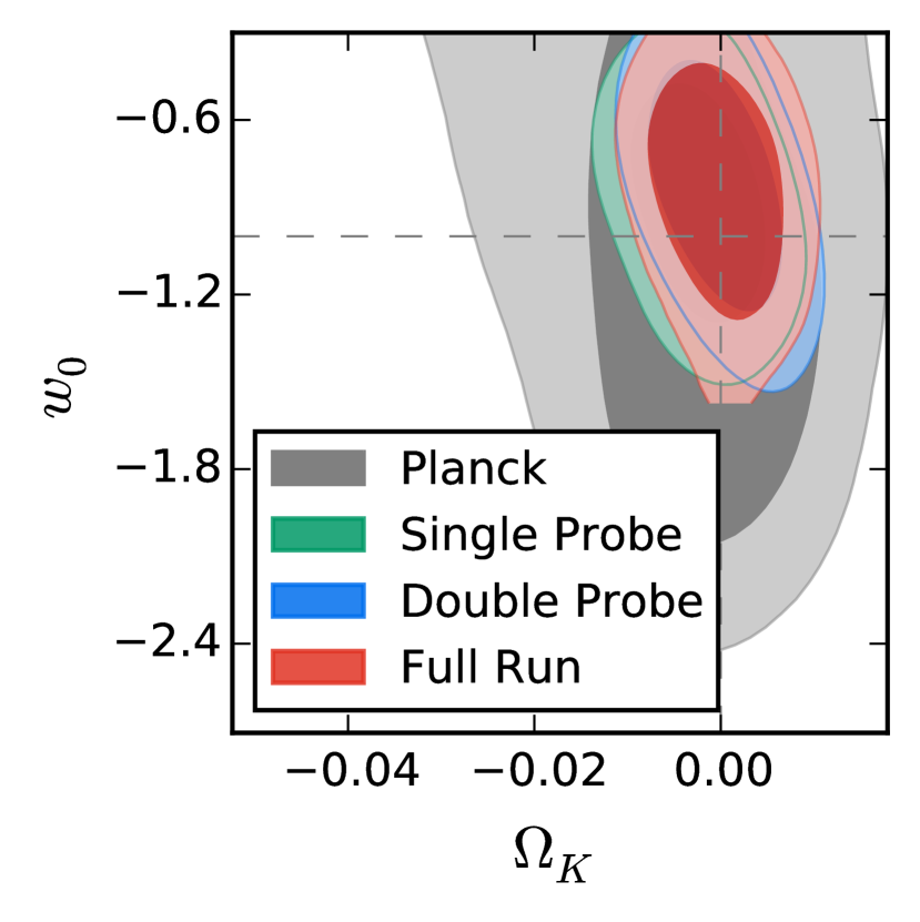
Table 3 lists the constraints on the parameters of different dark energy models obtained using our double-probe measurements. The results show no tension with the flat $\Lambda$CDM cosmological paradigm.

	$\Omega_{m}$	$H_{0}$	$\sigma_{8}$	$\Omega_{k}$	$w$ or $w_{0}$	$w_{a}$
$\Lambda$CDM	$0.304\pm 0.009$	$68.2\pm 0.7$	$0.806\pm 0.014$	$0$	$-1$	$0$
o$\Lambda$CDM	$0.303\pm 0.010$	$68.6\pm 0.9$	$0.810\pm 0.015$	$0.002\pm 0.003$	$-1$	$0$
$w$CDM	$0.299\pm 0.013$	$69.0\pm 1.5$	$0.815\pm 0.020$	$0$	$-1.04\pm 0.06$	$0$
o$w$CDM	$0.302\pm 0.014$	$68.7\pm 1.5$	$0.811\pm 0.021$	$0.002\pm 0.003$	$-1.00\pm 0.07$	$0$
$w_{0}w_{a}$CDM	$0.313\pm 0.020$	$67.6\pm 2.0$	$0.817\pm 0.016$	$0$	$-0.84\pm 0.22$	$-0.66\pm 0.68$
o$w_{0}w_{a}$CDM	$0.313\pm 0.020$	$67.6\pm 2.2$	$0.815\pm 0.016$	$0.000\pm 0.004$	$-0.85\pm 0.24$	$-0.61\pm 0.80$

Table 3: Constraints on cosmological parameters obtained by using our results assuming dark energy models (see Sec. 5).

6 Full-likelihood analysis Fixing Dark Energy Models

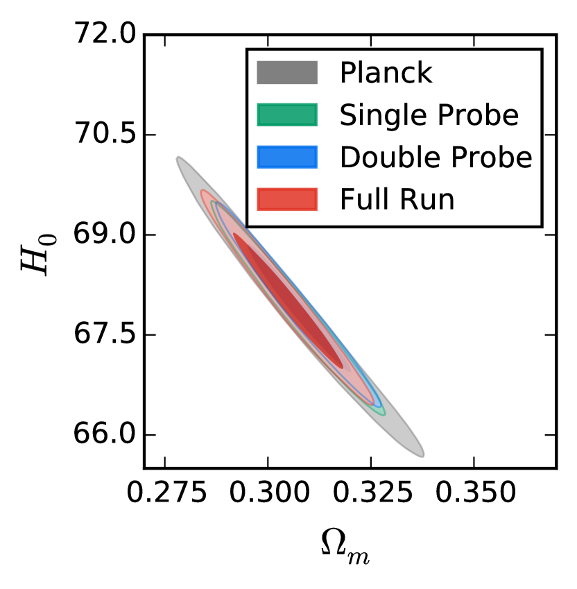
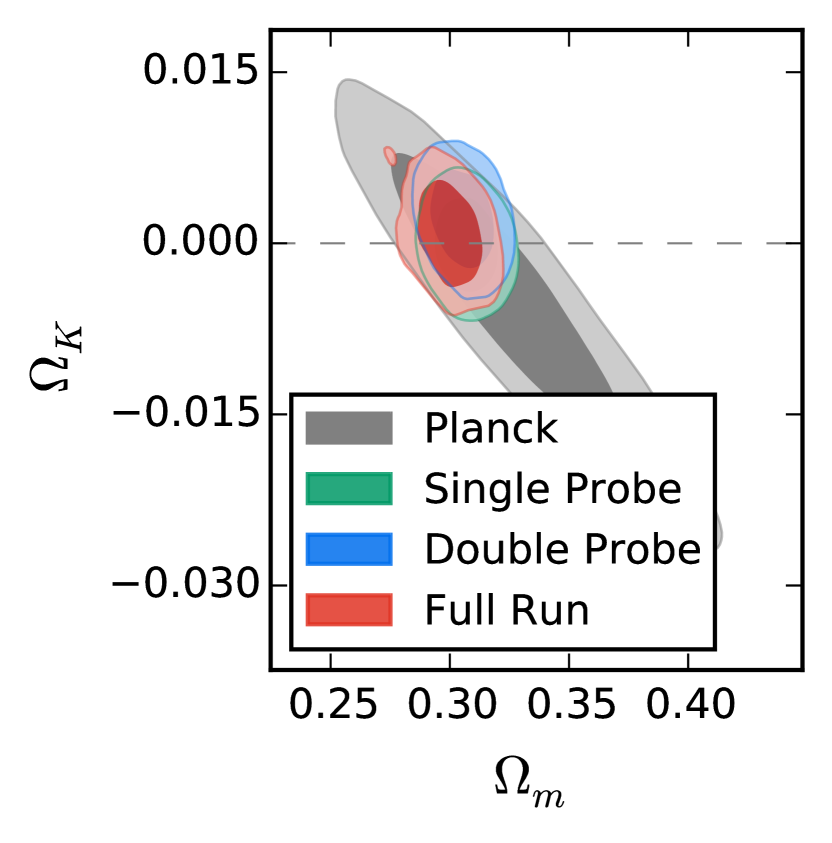
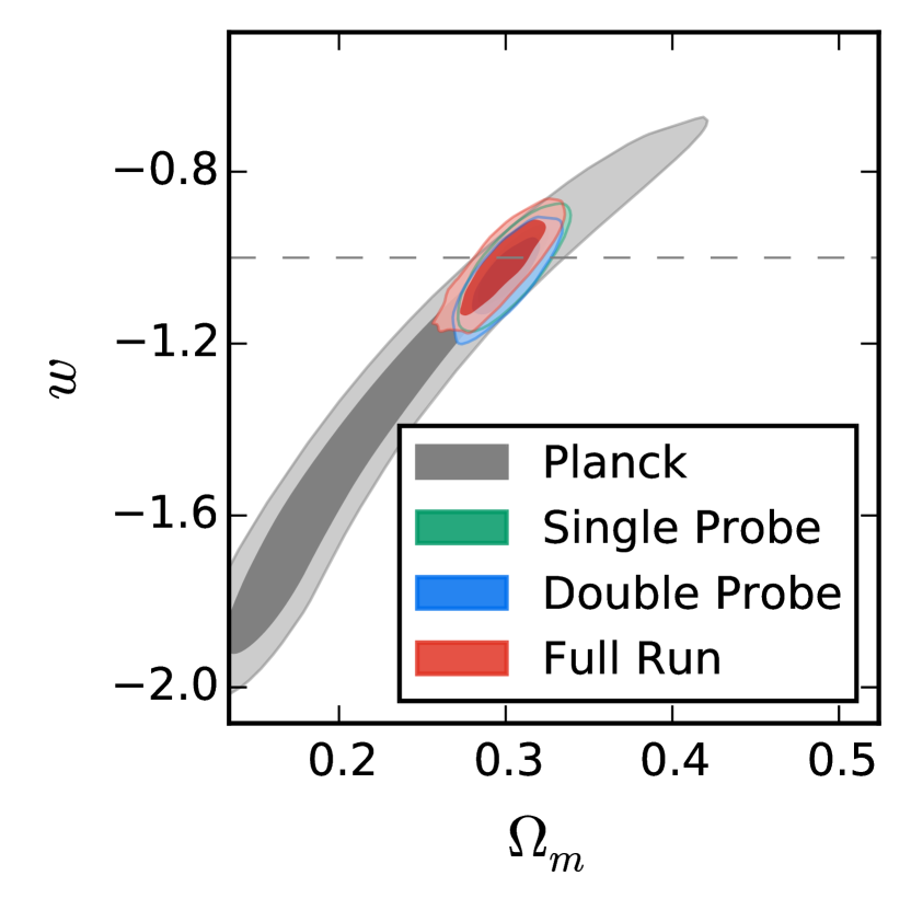
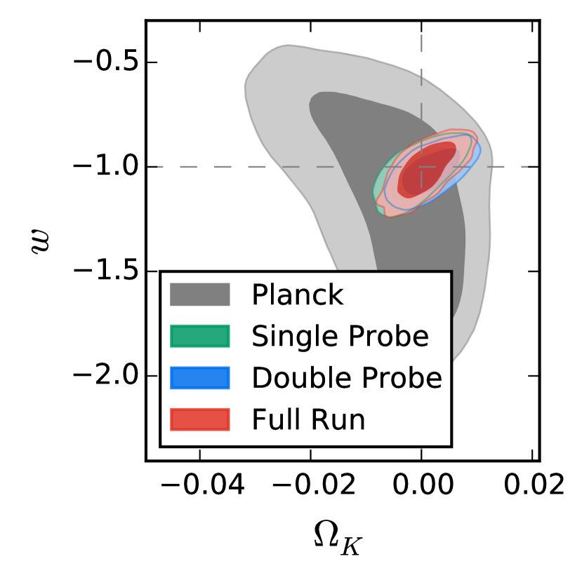
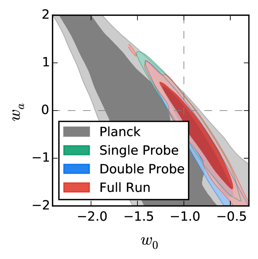
To validate our double-probe methodology, we perform the full-likelihood MCMC analyses with fixing dark energy models. The main difference of this approach comparing our double-probe analysis is that it has been given a dark energy model at first place. Opposite to the double probe approach, one cannot use the results from the full-likelihood analysis to derive the constraints for the parameters of other dark energy models. Since the dark energy model is fixed, the quantities, $\{H(z)$, $D_{A}(z)$, $\beta(z)$, $b\sigma_{8}(z)\}$, would be determined by the input parameters, $\{\Omega_{c}h^{2}$, $\Omega_{b}h^{2}$, $n_{s}$, $log(A_{s})$, $\theta$, $\tau$, $\Omega_{k}$, $w\}$, as shown in Eq. 24, 25, 27, and 31. We show the results in Table 4. In Fig. 3, 4 and 5, we compare these results with our double-probe approach and the single-probe approach (Chuang et al. (2016); companion paper). We find very good agreement among these three approaches. Note that deriving the dark energy model constraints from our double-probe measurements is much faster than the full run. For example, using the same machine, it takes $\sim 2.5$ hours to obtain the constraints for $\Lambda$CDM using double-probe measurements, but takes 6 days to reach similar convergence for the full likelihood MCMC analysis (slower with a factor of 60).

Up to this point we have introduced two methodologies for extracting cosmological information, the double-probe method and a full likelihood analysis. Moreover, we are comparing these results with a third methodology already introduced in Chuang et al. 2016 also called single-probe analysis combined with CMB. We show here motivations for the use of each of them:

• Double-probe: Joint fit to LSS data and CMB constraining the full set of cosmological parameters without the need of extra knowledge on the priors. This methodology allow us to test on the prior information content assumed by other probes and give us the tool to have a dark energy independent measurements from LSS and CMB combined.

• Full fit: Fit of cosmological parameter set to LSS and CMB data, requiring an assumption of a dark energy model (i.e. not going through $D_{A}$, $H$ and $f\sigma_{8}$ as intermediate parameters) from the beginning. This methodology provides a tool to check the information content of the data and we take it to be the answer to recover from other methodologies as it does not have extra assumptions appart from the dark energy model.

• Single-probe+CMB: Likelihoods are determined from the BOSS measurements of $\{D_{A}r_{s}^{fid}/r_{s}$, $Hr_{s}/r_{s}^{fid}$, $f\sigma_{8}$, $\Omega_{m}h^{2}\}$ together with Planck data. This methodology provides, in its first step, measurements of large scale structure independent of CMB data, thus showing as a good tool to test possible tensions between data sets.

	$\Omega_{m}$	$H_{0}$	$\sigma_{8}$	$\Omega_{k}$	$w$ or $w_{0}$	$w_{a}$
$\Lambda$CDM	$0.305\pm 0.008$	$68.0\pm 0.6$	$0.812\pm 0.009$	$0$	$-1$	$0$
o$\Lambda$CDM	$0.300\pm 0.009$	$68.6\pm 1.0$	$0.816\pm 0.010$	$0.001\pm 0.003$	$-1$	$0$
$w$CDM	$0.298\pm 0.015$	$68.8\pm 1.8$	$0.818\pm 0.017$	$0$	$-1.02\pm 0.07$	$0$
o$w$CDM	$0.298\pm 0.017$	$68.8\pm 1.8$	$0.818\pm 0.018$	$0.001\pm 0.003$	$-1.01\pm 0.08$	$0$
$w_{0}w_{a}$CDM	$0.311\pm 0.022$	$67.4\pm 2.3$	$0.808\pm 0.020$	$0$	$-0.85\pm 0.23$	$-0.51\pm 0.67$
o$w_{0}w_{a}$CDM	$0.309\pm 0.025$	$67.8\pm 3.0$	$0.810\pm 0.024$	$0.000\pm 0.004$	$-0.86\pm 0.26$	$-0.50\pm 0.73$

Table 4: Constraints on cosmological parameters from full-likelihood MCMC analysis of the joint data set (see Sec. 6).

Figure 3: Left panel: 2D marginalized contours for $68\%$ and $95\%$ confidence levels for $\Omega_{m}$ and $H_{0}$ ($\Lambda$CDM model assumed) from Planck-only (gray), derived using double probe measurements (blue), full -likelihood analysis with joint data (red; labeled as ”Full Run”), and Planck+single probe measurements (green). Right panel: 2D marginalized contours for $68\%$ and $95\%$ confidence level for $\Omega_{m}$ and $\Omega_{k}$ (o$\Lambda$CDM model assumed). One can see that the latter three measurements are consistent with each other.

Figure 4: Left panel: 2D marginalized contours for $68\%$ and $95\%$ confidence level for $\Omega_{m}$ and $w$ ($w$CDM model assumed) from Planck-only (gray), derived using double probe measurements (blue), full -likelihood analysis with joint data (red; labeled as ”Full Run”), and Planck+single probe measurements (green). Right panel: 2D marginalized contours for $68\%$ and $95\%$ confidence level for $\Omega_{k}$ and $w$ (o$w$CDM model assumed). One can see that the latter three measurements are consistent with each other.

Figure 5: Left panel: 2D marginalized contours for $68\%$ and $95\%$ confidence level for $w_{0}$ and $w_{a}$ ($w_{0}w_{a}$CDM model assumed) from Planck-only (gray), derived using double probe measurements (blue), full -likelihood analysis with joint data (red; labeled as ”Full Run”), and Planck+single probe measurements (green). Right panel: 2D marginalized contours for $68\%$ and $95\%$ confidence level for $\Omega_{k}$ and $w_{0}$ (o$w_{0}w_{a}$CDM model assumed). One can see that the latter three measurements are consistent with each other.

7 measurements of neutrino mass

In this section, we will focus on measuring the sum of the neutrino mass $\Sigma m_{\nu}$ using different methodologies described in previous sections. First, we repeat the double-probe analysis described in Sec. 3.3 with an additional free parameter, $\Sigma m_{\nu}$, and present the constraints on cosmological parameters. Second, we repeat the MCMC analysis with the full likelihood of joint data set described in Sec. 6 and find that the full shape measurement of the monopole of the galaxy 2-point correlation function introduces some detection of neutrino mass. However, since the monopole measurement is sensitive to the observational systematics, we provide another set of cosmological constraints by removing the full shape information. Third, we also obtain the constraint of $\Sigma m_{\nu}$ using the single probe measurement provided by Chuang et al. (companion paper).

7.1 measuring neutrino mass using double probe

Note first that for the study of $m_{\nu}$, we replace $R=\sqrt{\Omega_{m}H_{0}^{2}}\,r(z_{*})$ with $\Omega_{bc}h^{2}=\Omega_{b}h^{2}+\Omega_{c}h^{2}$ (e.g. see Aubourg et al. (2015)), since $R$ depends directly on $\Omega_{\nu}$. Thus, we use the following set of parameters from the double probe analysis while measuring neutrino mass, $\{\Omega_{bc}h^{2}$, $l_{a}$, $\Omega_{b}h^{2}$, $n_{s}$, $log(A_{s})$, $\Omega_{k}$, $H(z)$, $D_{A}(z)$, $f(z)\sigma_{8}(z)\}$.

We repeat the analysis described in Sec. 3.3, but here we set $\Sigma m_{\nu}$, to be free instead of setting it to $0.06$ eV. The results are shown in Table 5 and 6.

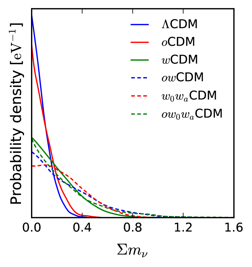
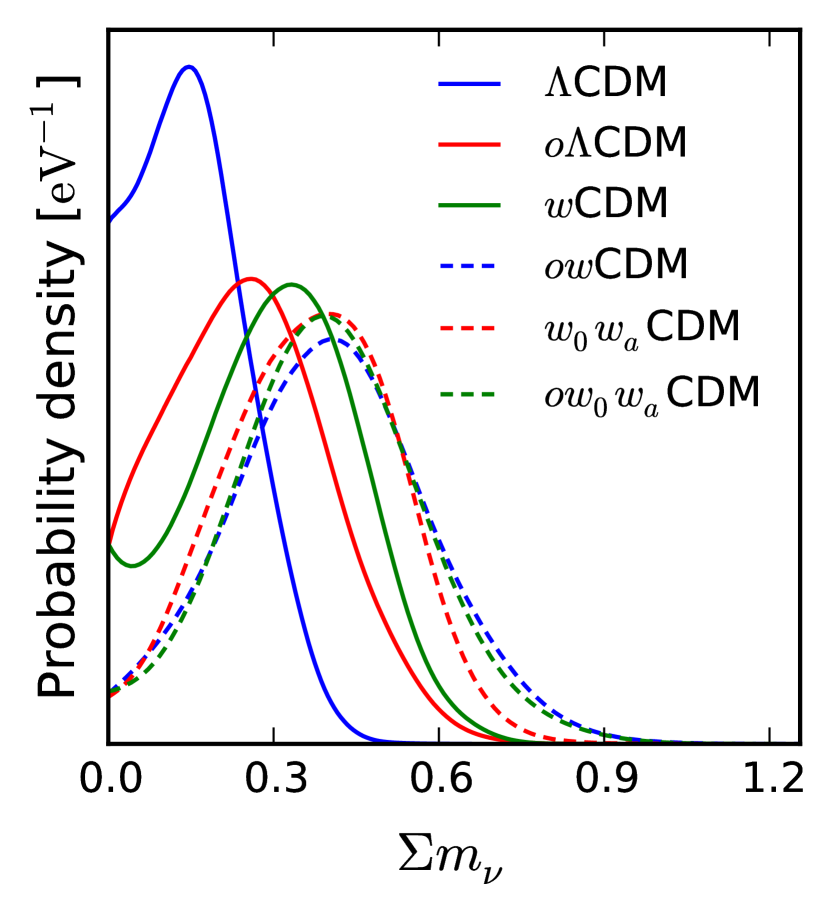
As described in Sec. 5, one can constrain the parameters of given dark energy models using Table 5 and 6. Table 7 presents the cosmological parameter constraints assuming some simple dark energy models. Figure 6 shows the probability density for $\Sigma m_{\nu}$ for different dark energy models. Our measurements of $\Sigma m_{\nu}$ using double probe approach are consistent with zero. The upper limit (68% confidence level) varys from 0.1 to 0.35 eV depending on dark energy model.

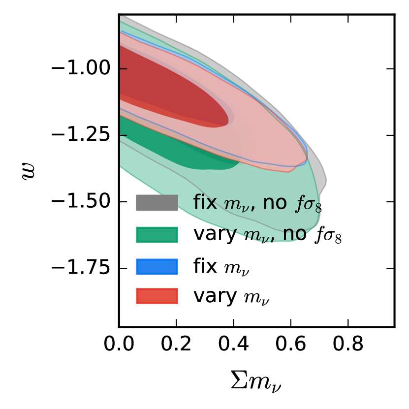
In addition, we also derive the cosmological constraints by using the results with fixed $\Sigma m_{\nu}$, i.e. Table 1 and 2 with $R$ replaced by $\Omega_{bc}h^{2}$. Different from Table 3 (see Sec. 5), we include $\Sigma m_{\nu}$ as one of the parameters to be constrained. The results are shown in Table 8. We find that the results are very similar to Table 7, which showing our double probe measurements are insensitive to the $\Sigma m_{\nu}$ assumption. Fig. 7 shows this point in a clear way by comparing the 2D contours when including a covariance matrix varying $\Sigma m_{\nu}$ (using Table 5 and 6) or fixing $\Sigma m_{\nu}$ (using Table 1 and 2). We see that they lie on top of each other. Moreover, Fig. 7 also exhibit the constraint given by $f\sigma_{8}$ on the $\Sigma m_{\nu}$ and $w$ parameters. We find the constraint on $w$ become tighter while that in $\Sigma m_{\nu}$ stays the same when including the $f\sigma_{8}$ constraint. This is a good news for future experiments as their power on the neutrino constraint would not highly rely on the growth rate measurements which are more sensitive to the observational systematics.

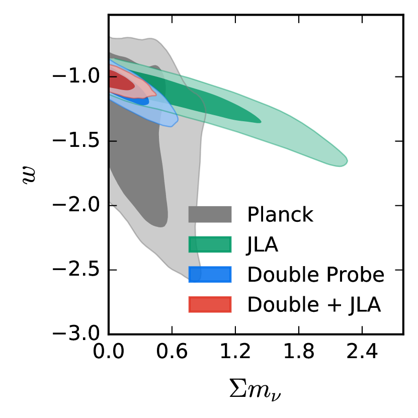
Furthermore, we have also checked the impact of adding supernovae Ia (SNIa) data, dubbed Joint Light-curve Analysis (JLA) (Betoule et al., 2014) and find that the upper limit of $\Sigma m_{\nu}$ decrease because SNIa breaks the degeneracy of the constraint from Planck+BOSS (see Fig. 8). In this way, we can get tighter constraints on the upper limit by including SNIa data.

$f\sigma_{8}(0.59)$	$0.495\pm 0.051$
$H(0.59)r_{s}/r_{s,fid}$	$97.5\pm 3.2$
$D_{A}(0.59)r_{s,fid}/r_{s}$	$1419\pm 27$
$f\sigma_{8}(0.32)$	$0.431\pm 0.066$
$H(0.32)r_{s}/r_{s,fid}$	$78.9\pm 3.6$
$D_{A}(0.32)r_{s,fid}/r_{s}$	$964\pm 26$
$\Omega_{bc}h^{2}$	$0.1413\pm 0.0022$
$l_{a}$	$301.75\pm 0.14$
$\Omega_{b}h^{2}$	$0.02209\pm 0.00025$
$n_{s}$	$0.9639\pm 0.0068$
${\rm{ln}}(10^{10}A_{s})$	$3.062\pm 0.040$
$\Omega_{k}$	$-0.009\pm 0.006$

Table 5: Results of double-probe analysis obtained with varying $\Sigma m_{\nu}$. The units of $H(z)$ and $D_{A}(z)$ are $\,{\rm km}\,{\rm s}^{-1}\,{\rm Mpc}^{-1}$ and Mpc (see Sec. 7.1).

	$\Omega_{bc}h^{2}$	$l_{a}$	$\Omega_{b}h^{2}$	$n_{s}$	${\rm{ln}}(10^{10}A_{s})$	$f\sigma_{8}(0.59)$	$\frac{H(0.59)}{r_{s,fid}/r_{s}}$	$\frac{D_{A}(0.59)}{r_{s}/r_{s,fid}}$	$f\sigma_{8}(0.32)$	$\frac{H(0.32)}{r_{s,fid}/r_{s}}$	$\frac{D_{A}(0.32)}{r_{s}/r_{s,fid}}$	$\Omega_{k}$
$\Omega_{bc}h^{2}$	1.0000	0.4607	-0.6377	-0.8376	0.0145	0.0075	0.0536	0.0672	-0.0870	0.0317	0.0049	0.3794
$l_{a}$	0.4607	1.0000	-0.4977	-0.5042	-0.0470	0.0201	-0.0525	0.0043	-0.0216	0.0765	0.0912	0.2919
$\Omega_{b}h^{2}$	-0.6377	-0.4977	1.0000	0.7188	-0.0241	-0.0016	-0.0625	-0.0879	0.0692	0.0299	0.0149	-0.2708
$n_{s}$	-0.8376	-0.5042	0.7188	1.0000	0.0475	-0.0131	-0.0591	-0.0499	0.0717	0.0268	-0.0686	-0.2894
${\rm{ln}}(10^{10}A_{s})$	0.0145	-0.0470	-0.0241	0.0475	1.0000	0.0095	-0.0352	-0.0065	0.0773	0.0225	0.0053	0.5576
$f\sigma_{8}(0.59)$	0.0075	0.0201	-0.0016	-0.0131	0.0095	1.0000	0.6546	0.5223	0.2427	0.2074	0.0634	0.1538
$H(0.59)r_{s}/r_{s,fid}$	0.0536	-0.0525	-0.0625	-0.0591	-0.0352	0.6546	1.0000	0.3777	0.0586	0.0615	0.0015	-0.0025
$D_{A}(0.59)r_{s,fid}/r_{s}$	0.0672	0.0043	-0.0879	-0.0499	-0.0065	0.5223	0.3777	1.0000	-0.0598	0.0272	-0.0474	-0.0578
$f\sigma_{8}(0.32)$	-0.0870	-0.0216	0.0692	0.0717	0.0773	0.2427	0.0586	-0.0598	1.0000	0.6531	0.4819	0.1487
$H(0.32)r_{s}/r_{s,fid}$	0.0317	0.0765	0.0299	0.0268	0.0225	0.2074	0.0615	0.0272	0.6531	1.0000	0.1686	0.1165
$D_{A}(0.32)r_{s,fid}/r_{s}$	0.0049	0.0912	0.0149	-0.0686	0.0053	0.0634	0.0015	-0.0474	0.4819	0.1686	1.0000	0.0049
$\Omega_{k}$	0.3794	0.2919	-0.2708	-0.2894	0.5576	0.1538	-0.0025	-0.0578	0.1487	0.1165	0.0049	1.0000

Table 6: Correlation matrix of the double-probe measurements obtained with varying $\Sigma m_{\nu}$ (corresponding to Table 5; see Sec. 7.1).

	$\Omega_{m}$	$H_{0}$	$\sigma_{8}$	$\Omega_{k}$	$w$ or $w_{0}$	$w_{a}$	$\Sigma{m_{\mu}}$(eV)
$\Lambda$CDM	$0.310\pm 0.010$	$67.6\pm 0.8$	$0.828\pm 0.019$	$0$	$-1$	$0$	$<0.10$ $(<0.22)$
o$\Lambda$CDM	$0.310\pm 0.011$	$67.8\pm 1.0$	$0.828\pm 0.020$	$0.002\pm 0.003$	$-1$	$0$	$<0.13$ $(<0.27)$
$w$CDM	$0.296\pm 0.016$	$69.6\pm 1.9$	$0.824\pm 0.027$	$0$	$-1.11\pm 0.10$	$0$	$<0.26$ $(<0.52)$
o$w$CDM	$0.297\pm 0.017$	$69.8\pm 2.2$	$0.816\pm 0.033$	$0.001\pm 0.004$	$-1.13\pm 0.12$	$0$	$<0.35$ $(<0.75)$
$w_{0}w_{a}$CDM	$0.312\pm 0.024$	$68.1\pm 2.6$	$0.812\pm 0.030$	$0$	$-0.88\pm 0.24$	$-0.89\pm 0.75$	$<0.32$ $(<0.60)$
o$w_{0}w_{a}$CDM	$0.310\pm 0.026$	$68.3\pm 3.3$	$0.809\pm 0.034$	$-0.001\pm 0.004$	$-0.91\pm 0.29$	$-0.83\pm 0.87$	$<0.31$ $(<0.78)$

Table 7: Constraints on cosmological parameters obtained by using the double-probe measurements presented in Table 5 and 6 assuming dark energy models. We show 68% 1-D marginalized constraints for all the parameters. We provide also 95% constraints for the neutrino masses in the parentheses. The units of $H_{0}$ and $\Sigma m_{\nu}$ are $\,{\rm km}\,{\rm s}^{-1}\,{\rm Mpc}^{-1}$ and eV respectively (see Sec. 7.1 and Fig. 6).

Figure 6: Probability density for $\Sigma m_{\nu}$ from double-probe measurements using the covariance matrix with free parameter $\Sigma m_{\nu}$ (see Sec. 7.1 and Table 7).

	$\Omega_{m}$	$H_{0}$	$\sigma_{8}$	$\Omega_{k}$	$w$ or $w_{0}$	$w_{a}$	$\Sigma{m_{\mu}}$(eV)
$\Lambda$CDM	$0.306\pm 0.009$	$68.0\pm 0.7$	$0.803\pm 0.017$	$0$	$-1$	$0$	$<0.12$ $(<0.24)$
o$\Lambda$CDM	$0.307\pm 0.010$	$68.2\pm 0.9$	$0.796\pm 0.021$	$0.003\pm 0.003$	$-1$	$0$	$<0.19$ $(<0.37)$
$w$CDM	$0.295\pm 0.014$	$69.5\pm 1.8$	$0.798\pm 0.023$	$0$	$-1.10\pm 0.10$	$0$	$<0.27$ $(<0.53)$
o$w$CDM	$0.296\pm 0.015$	$70.1\pm 2.3$	$0.781\pm 0.033$	$0.003\pm 0.004$	$-1.13\pm 0.14$	$0$	$<0.45$ $(<0.91)$
$w_{0}w_{a}$CDM	$0.307\pm 0.020$	$68.5\pm 2.3$	$0.782\pm 0.028$	$0$	$-0.92\pm 0.22$	$-0.77\pm 0.73$	$<0.39$ $(<0.63)$
o$w_{0}w_{a}$CDM	$0.302\pm 0.021$	$69.4\pm 2.8$	$0.775\pm 0.034$	$0.002\pm 0.004$	$-1.01\pm 0.28$	$-0.53\pm 0.88$	$<0.47$ $(<0.93)$

Table 8: Constraints on cosmological parameters obtained by using our double-probe measurements obtained with fixed $\Sigma m_{\nu}$ assuming dark energy models. We show 68% 1-D marginalized constraints for all the parameters. We provide also 95% constraints for the neutrino masses in the parentheses. The units of $H_{0}$ and $\Sigma m_{\nu}$ are $\,{\rm km}\,{\rm s}^{-1}\,{\rm Mpc}^{-1}$ and eV respectively. One can see that the results are very similar to Table 7, which showing our double probe measurements are insensitive to the $\Sigma m_{\nu}$ assumption

Figure 7: Comparison of 2D contours for $68\%$ and $95\%$ confidence level on $\Sigma m_{\nu}$ and $w$ from the double probe methodology using covariance matrix from first step varying and fixing neutrinos. One can see that the constraints are insensitive to the assumption of $\Sigma m_{\nu}$. We also show the results from double probe measurement excluding $f(z)\sigma_{8}(z)$. One can see that $f(z)\sigma_{8}(z)$ improve the constraint on $w$ but not $\Sigma m_{\nu}$.

Figure 8: 2D marginalized contours for $68\%$ and $95\%$ confidence level for $w$ and $\Sigma m_{\nu}$ ($w$CDM model assumed) from Planck-only (gray), double-probe (blue), JLA (green), and double probe + JLA (red).

7.2 measuring neutrino mass using full likelihood analysis

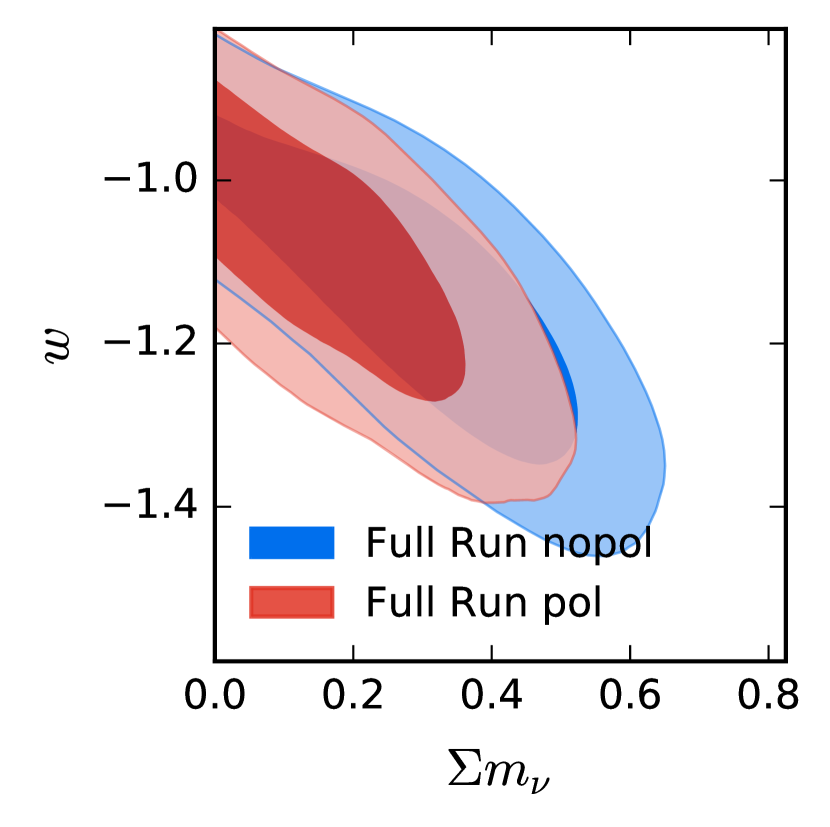
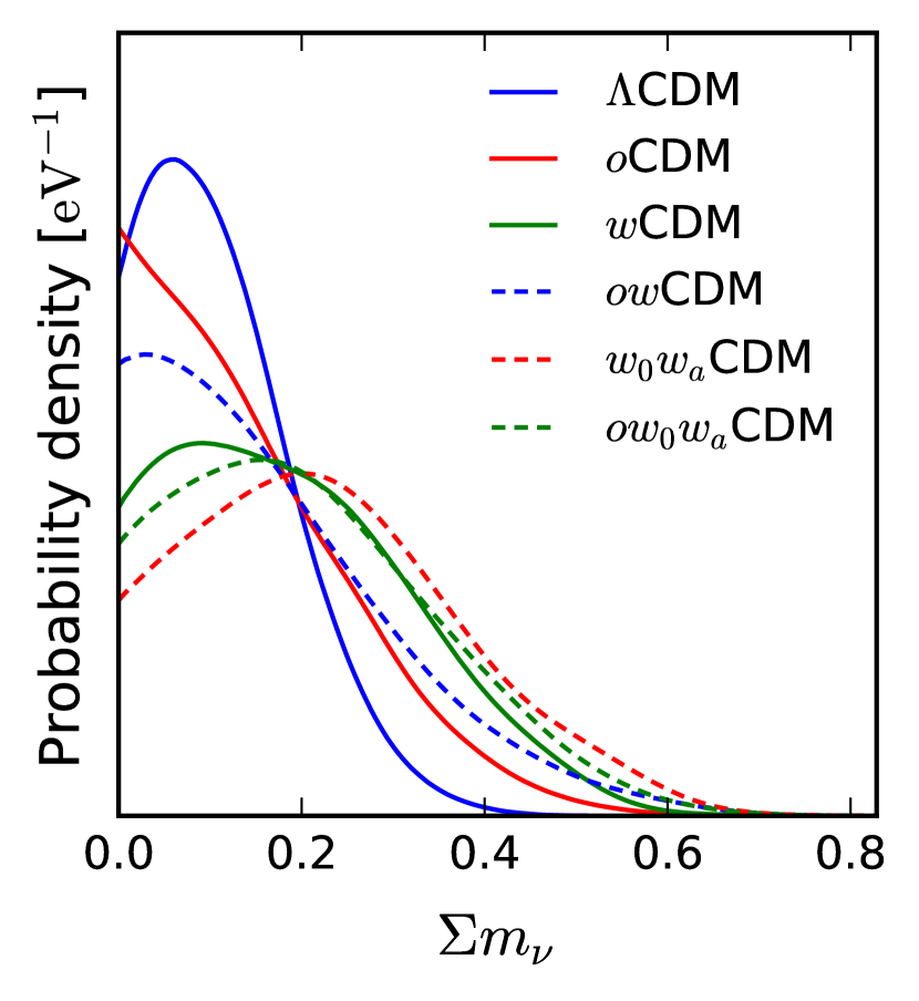
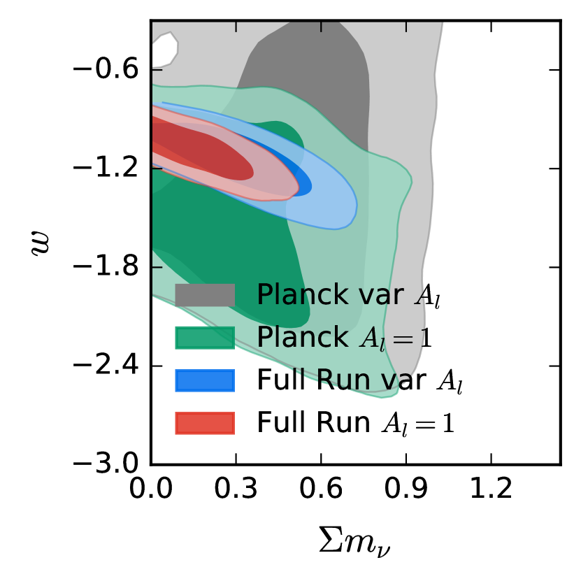
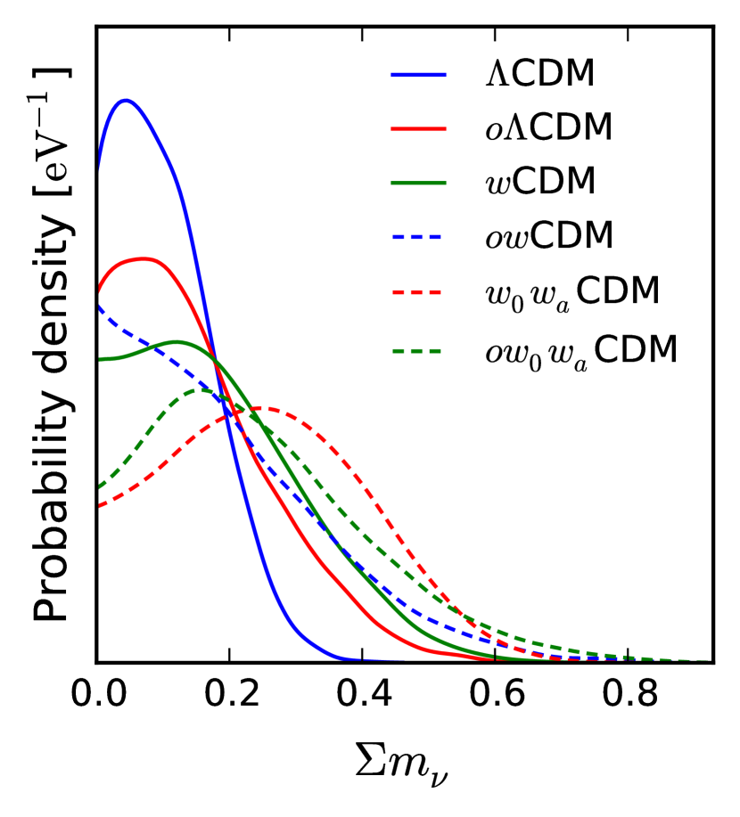
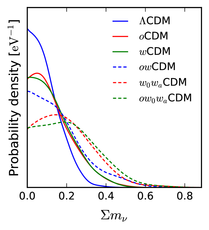
We perform the same full MCMC analysis using the joint-full-likelihood of Planck and BOSS data as described in Sec. 6 to obtain the cosmological parameter constraints including $\Sigma m_{\nu}$. Table 9 presents the results. We show also the probability density for $\Sigma m_{\nu}$ in Fig. 9. We find more than 2 $\sigma$ detection of non zero $\Sigma m_{\nu}$ assuming the models without fixing $w$ to be -1. However, we find that the detection actually mainly comes from the monopole of galaxy correlation function which is sensitive to some observational systematics, e.g. see Ross et al. (2012); Chuang et al. (2013b). Fig. 10 shows that the $\Sigma m_{\nu}$ detection decreases when adding a polynomial to remove the full shape information of monopole. To be conservative, we run again the full MCMC analysis to obtain the constraint on $\Sigma m_{\nu}$ without including the full shape information and the results are presented in Table 10. The probability density for $\Sigma m_{\nu}$ is shown in Fig. 11. One can see the detections of $\Sigma m_{\nu}$ decrease. In addition, the upper limits in Fig. 11 are lower than Fig. 6 which are expected. Since we do not include the parameter $\Sigma m_{\nu}$ when summarising the information of double probe, the $\Sigma m_{\nu}$ constraint from $Planck$ is lost.

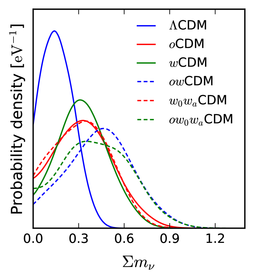
Table 11 displays the constraints measured when allowing the CMB lensing amplitude parameter $A_{\rm L}$ to vary. Fig. 13 shows the $Planck$ data shifts $\Sigma m_{\nu}$ measurement to higher values allowing a higher detection from the combined data analysis when allowing $A_{\rm L}$ free. Thus, we find again $\sim$ 2 $\sigma$ detection even without accounting for the full shape of the monopole from the correlation function.

	$\Omega_{m}$	$H_{0}$	$\sigma_{8}$	$\Omega_{k}$	$w$ or $w_{0}$	$w_{a}$	$\Sigma{m_{\mu}}$(eV)
$\Lambda$CDM	$0.308\pm 0.011$	$67.7\pm 0.9$	$0.801\pm 0.017$	$0$	$-1$	$0$	$<0.22$ $(<0.32)$
o$\Lambda$CDM	$0.313\pm 0.013$	$67.9\pm 1.1$	$0.792\pm 0.020$	$0.004\pm 0.004$	$-1$	$0$	$0.25_{-0.17}^{+0.13}$ $(<0.49)$
$w$CDM	$0.293\pm 0.016$	$70.1\pm 2.0$	$0.808\pm 0.019$	$0$	$-1.15\pm 0.11$	$0$	$0.30_{-0.14}^{+0.17}$ $(<0.52)$
o$w$CDM	$0.299\pm 0.019$	$70.0\pm 2.4$	$0.795\pm 0.021$	$0.004\pm 0.004$	$-1.14\pm 0.13$	$0$	$0.40_{-0.17}^{+0.17}$ $\left({}_{-0.33}^{+0.34}\right)$
$w_{0}w_{a}$CDM	$0.316\pm 0.023$	$67.8\pm 2.5$	$0.785\pm 0.023$	$0$	$-0.87\pm 0.23$	$-0.96\pm 0.68$	$0.36_{-0.15}^{+0.17}$ $\left({}_{-0.29}^{+0.26}\right)$
o$w_{0}w_{a}$CDM	$0.313\pm 0.026$	$68.4\pm 2.8$	$0.787\pm 0.027$	$0.002\pm 0.004$	$-0.91\pm 0.26$	$-0.82\pm 0.77$	$0.39_{-0.15}^{+0.15}$ $\left({}_{-0.32}^{+0.32}\right)$

Table 9: Constraints on cosmological parameters from the full-likelihood-analysis of the joint data set. $\Sigma m_{\nu}$ is one of the parameters to be constrained. Planck data includes lensing with $A_{\rm L}=1$. The overall shape information of the monopole of the correlation function from the BOSS galaxy clustering is included. We show 68% 1-D marginalized constraints for all the parameters. We provide also 95% constraints for the neutrino masses in the parentheses. The units of $H_{0}$ and $\Sigma m_{\nu}$ are $\,{\rm km}\,{\rm s}^{-1}\,{\rm Mpc}^{-1}$ and eV respectively (see Sec. 7.2 and Fig. 9).

Figure 9: Probability density for $\Sigma m_{\nu}$ from the full-likelihood-analysis of the joint data set. $\Sigma m_{\nu}$ is one of the parameters to be constrained. Planck data including lensing with $A_{\rm L}=1$. The overall shape information of the monopole of the correlation function from the BOSS galaxy clustering is included (see Sec. 7.2 and Table 9).

Figure 10: 2D marginalized contours for $68\%$ and $95\%$ confidence level for $w$ and $\Sigma m_{\nu}$ ($w$CDM model assumed) from Planck+BOSS. The blue contours are from full-likelihood-analysis without using a polynomial function to remove the overall shape information of monopole; the red contours are from the analysis removing overall shape information with a polynomial function. One can see that the overall shape information shift the $\Sigma m_{\nu}$ to a larger value.

	$\Omega_{m}$	$H_{0}$	$\sigma_{8}$	$\Omega_{k}$	$w$ or $w_{0}$	$w_{a}$	$\Sigma{m_{\mu}}$(eV)
$\Lambda$CDM	$0.309\pm 0.011$	$67.7\pm 0.9$	$0.808\pm 0.015$	$0$	$-1$	$0$	$<0.14$ $(<0.26)$
o$\Lambda$CDM	$0.310\pm 0.012$	$67.9\pm 1.0$	$0.805\pm 0.017$	$0.002\pm 0.003$	$-1$	$0$	$<0.18$ $(<0.36)$
$w$CDM	$0.296\pm 0.017$	$69.6\pm 2.1$	$0.818\pm 0.021$	$0$	$-1.11\pm 0.11$	$0$	$<0.25$ $(<0.42)$
o$w$CDM	$0.300\pm 0.019$	$69.1\pm 2.2$	$0.813\pm 0.021$	$0.001\pm 0.004$	$-1.08\pm 0.12$	$0$	$<0.21$ $(<0.43)$
$w_{0}w_{a}$CDM	$0.312\pm 0.027$	$68.2\pm 3.1$	$0.803\pm 0.028$	$0$	$-0.91\pm 0.27$	$-0.70\pm 0.79$	$<0.33$ $(<0.49)$
o$w_{0}w_{a}$CDM	$0.311\pm 0.025$	$68.0\pm 2.7$	$0.803\pm 0.026$	$0.000\pm 0.004$	$-0.92\pm 0.25$	$-0.59\pm 0.78$	$<0.28$ $(<0.45)$

Table 10: Constraints on cosmological parameters from the full-likelihood-analysis of the joint data set. $\Sigma m_{\nu}$ is one of the parameters to be constrained. Planck data includes lensing with $A_{\rm L}=1$. The overall shape information of the monopole of the correlation function from the BOSS galaxy clustering is removed with a polynomial function. We show 68% 1-D marginalized constraints for all the parameters. We provide also 95% constraints for the neutrino masses in the parentheses. The units of $H_{0}$ and $\Sigma m_{\nu}$ are $\,{\rm km}\,{\rm s}^{-1}\,{\rm Mpc}^{-1}$ and eV respectively (see Sec. 7.2 and Fig. 11).

Figure 11: Probability density for $\Sigma m_{\nu}$ from the full-likelihood-analysis of the joint data set. $\Sigma m_{\nu}$ is one of the parameters to be constrained. Planck data includes lensing with $A_{\rm L}=1$. The overall shape information of the monopole of the correlation function from the BOSS galaxy clustering is removed with a polynomial function (see Sec. 7.2 and Table 10).

	$\Omega_{m}$	$H_{0}$	$\sigma_{8}$	$\Omega_{k}$	$w$ or $w_{0}$	$w_{a}$	$\Sigma{m_{\mu}}$(eV)	$A_{L}$
$\Lambda$CDM	$0.308\pm 0.011$	$67.7\pm 0.9$	$0.782\pm 0.026$	$0$	$-1$	$0$	$0.17_{-0.13}^{+0.08}$ $(<0.34)$	$1.07\pm 0.06$
o$\Lambda$CDM	$0.314\pm 0.013$	$67.9\pm 1.0$	$0.752\pm 0.037$	$0.005\pm 0.004$	$-1$	$0$	$0.34_{-0.22}^{+0.17}$ $(<0.66)$	$1.12\pm 0.07$
$w$CDM	$0.290\pm 0.019$	$70.4\pm 2.5$	$0.781\pm 0.032$	$0$	$-1.16\pm 0.14$	$0$	$0.33_{-0.18}^{+0.16}$ $(<0.60)$	$1.10\pm 0.07$
o$w$CDM	$0.300\pm 0.023$	$69.8\pm 2.8$	$0.754\pm 0.041$	$0.005\pm 0.005$	$-1.11\pm 0.15$	$0$	$0.44_{-0.22}^{+0.23}$ $(<0.81)$	$1.13\pm 0.07$
$w_{0}w_{a}$CDM	$0.292\pm 0.031$	$70.4\pm 3.9$	$0.781\pm 0.037$	$0$	$-1.15\pm 0.34$	$-0.09\pm 0.94$	$0.32_{-0.20}^{+0.18}$ $(<0.61)$	$1.10\pm 0.06$
o$w_{0}w_{a}$CDM	$0.292\pm 0.030$	$70.8\pm 3.7$	$0.763\pm 0.044$	$0.004\pm 0.005$	$-1.18\pm 0.32$	$0.11\pm 0.94$	$0.42_{-0.22}^{+0.22}$ $(<0.77)$	$1.14\pm 0.09$

Table 11: Constraints on cosmological parameters from the full-likelihood-analysis from the joint data set. Both $\Sigma m_{\nu}$ and $A_{\rm L}$ are the parameters to be constrained. The overall shape information of the monopole of the correlation function from the BOSS galaxy clustering is removed with a polynomial function. We show 68% 1-D marginalized constraints for all the parameters. We provide also 95% constraints for the neutrino masses in the parentheses. The units of $H_{0}$ and $\Sigma m_{\nu}$ are $\,{\rm km}\,{\rm s}^{-1}\,{\rm Mpc}^{-1}$ and eV respectively (see Sec. 7.2 and Fig. 12).

Figure 12: Probability density for $\Sigma m_{\nu}$ from full-likelihood-analysis from the joint data set. Both $\Sigma m_{\nu}$ and $A_{\rm L}$ are the parameters to be constrained. The overall shape information of the monopole of the correlation function from the BOSS galaxy clustering is removed with a polynomial function (see Sec. 7.2 and Table 11). One can see that the maximum of $\Sigma m_{\nu}$ increases comparing to the cases with fixing $A_{\rm L}=1$ (see Fig. 11).

Figure 13: 2D marginalized contours for $68\%$ and $95\%$ confidence level for $w$ and $\Sigma m_{\nu}$ ($w$CDM model assumed) from full run methodology and Planck only for different lensing information used. Gray contours and green contours are from Planck only with varying $A_{\rm L}$ and fixing $A_{\rm L}=1$ respectively; the blue contours and the red contours are from Planck+BOSS with varying $A_{\rm L}$ and fixing $A_{\rm L}=1$ respectively using full-likelihood-analysis. One can see that $\Sigma m_{\nu}$ shift to a large value when varying $A_{\rm L}$ for both data combinations.

7.3 measure neutrino mass using measurements from single probe analysis

We use the single probe measurement provided by Chuang et al. (companion paper) combining with Planck (fixing $A_{\rm L}=1$) and obtain the constraint of $\Sigma m_{\nu}$. Table 12 shows the cosmological parameter constraints including $\Sigma m_{\nu}$ for different dark energy models. The probability densities for $\Sigma m_{\nu}$ are shown in Fig. 14. One can see that it is consistent with Fig. 11. We have checked that there would be some detection of neutrino mass while allowing $A_{\rm L}$ to be free as seen in the case of full-likelihood analysis (see Sec. 7.2).

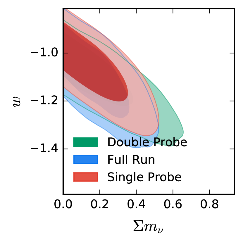
Fig. 15 presents the comparison between the three different methodologies. The three approaches agree very well with some subtle differences. One can see that the constraint on $\Sigma m_{\nu}$ from the double probe approach is weaker which is expected. The difference comes from the fact that we do not include $\Sigma m_{\nu}$ into our summarized set of parameters, so that information from $Planck$ is lost. On the other hand, both single probe and full-likelihood analysis include full $Planck$ information and their measurements are very similar.

	$\Omega_{m}$	$H_{0}$	$\sigma_{8}$	$\Omega_{k}$	$w$ or $w_{0}$	$w_{a}$	$\Sigma{m_{\mu}}$(eV)
$\Lambda$CDM	$0.310\pm 0.010$	$67.6\pm 0.8$	$0.809\pm 0.014$	$0$	$-1$	$0$	$<0.14$ $(<0.24)$
o$\Lambda$CDM	$0.313\pm 0.011$	$67.6\pm 0.9$	$0.804\pm 0.016$	$0.002\pm 0.004$	$-1$	$0$	$<0.19$ $(<0.37)$
$w$CDM	$0.303\pm 0.014$	$68.7\pm 1.7$	$0.812\pm 0.017$	$0$	$-1.08\pm 0.09$	$0$	$<0.24$ $(<0.42)$
o$w$CDM	$0.305\pm 0.014$	$68.6\pm 1.6$	$0.809\pm 0.018$	$0.001\pm 0.004$	$-1.06\pm 0.10$	$0$	$<0.25$ $(<0.48)$
$w_{0}w_{a}$CDM	$0.314\pm 0.021$	$67.8\pm 2.2$	$0.800\pm 0.022$	$0$	$-0.91\pm 0.22$	$-0.70\pm 0.75$	$0.26_{-0.18}^{+0.13}$ $(<0.51)$
o$w_{0}w_{a}$CDM	$0.315\pm 0.020$	$67.6\pm 2.1$	$0.799\pm 0.022$	$-0.001\pm 0.004$	$-0.89\pm 0.21$	$-0.77\pm 0.74$	$0.24_{-0.22}^{+0.08}$ $(<0.55)$

Table 12: The cosmological constraints including total mass of neutrinos from the single probe measurements provided by Chuang et al. 2016 (companion paper) combining with Planck data assuming different dark energy models. We show 68% 1-D marginalized constraints for all the parameters. We provide also 95% constraints for the neutrino masses in the parentheses. The units of $H_{0}$ and $\Sigma m_{\nu}$ are $\,{\rm km}\,{\rm s}^{-1}\,{\rm Mpc}^{-1}$ and eV respectively (see Sec. 7.2 and Fig.14).

Figure 14: Probability density for $\Sigma m_{\nu}$ from the single probe measurements provided by Chuang et al. 2016 (companion paper) combining with Planck data (with fixing $A_{\rm L}=1$). All the measurements are consistent with $\Sigma m_{\nu}=0$ (see Sec. 7.2 and Table 12).

Figure 15: Comparison of 2D contours for $68\%$ and $95\%$ confidence level on $\Sigma m_{\nu}$ and $w$ from the double probe, single probe, and full-likelihood-analysis approaches. One can see that the constraint on $\Sigma m_{\nu}$ from the double probe approach is weaker which is expected. The difference comes from the fact that we do not include $\Sigma m_{\nu}$ into our summarized set of parameters, so information from $Planck$ is lost.

7.4 combination with supernovae type Ia data

We combine our measurements using the full likelihood approach with those from supernovae Ia (SNIa) data, Joint Light-curve Analysis (JLA) (Betoule et al., 2014). As seen in Fig. 8, SN data breaks some degeneracies providing tighter constraints on $\Sigma m_{\nu}$. Results can be found in table 13 and Fig. 16) for the case of fixing $A_{\rm L}=1$ and table 14 and Fig. 17) for the case of varying $A_{\rm L}$. When adding SN1a data, we get tighter upper limits, e.g. $\Sigma m_{\nu}<0.12$ against $\Sigma m_{\nu}<0.14$ in $\Lambda CDM$ with $A_{\rm L}=1$. We point out that the constraints we obtained are still not sufficient to distinguish between normal and inverted hierarchy.

	$\Omega_{m}$	$H_{0}$	$\sigma_{8}$	$\Omega_{k}$	$w$ or $w_{0}$	$w_{a}$	$\Sigma{m_{\mu}}$(eV)
$\Lambda$CDM	$0.309\pm 0.010$	$67.7\pm 0.8$	$0.810\pm 0.014$	$0$	$-1$	$0$	$<0.12$ $(<0.24)$
o$\Lambda$CDM	$0.309\pm 0.010$	$67.9\pm 0.9$	$0.807\pm 0.016$	$0.001\pm 0.004$	$-1$	$0$	$<0.17$ $(<0.33)$
$w$CDM	$0.305\pm 0.012$	$68.2\pm 1.2$	$0.812\pm 0.016$	$0$	$-1.04\pm 0.05$	$0$	$<0.17$ $(<0.33)$
o$w$CDM	$0.307\pm 0.013$	$68.3\pm 1.4$	$0.808\pm 0.019$	$0.001\pm 0.004$	$-1.03\pm 0.06$	$0$	$<0.20$ $(<0.43)$
$w_{0}w_{a}$CDM	$0.309\pm 0.014$	$68.2\pm 1.3$	$0.807\pm 0.019$	$0$	$-0.92\pm 0.12$	$-0.64\pm 0.56$	$<0.26$ $(<0.43)$
o$w_{0}w_{a}$CDM	$0.310\pm 0.013$	$68.0\pm 1.3$	$0.803\pm 0.019$	$0.000\pm 0.004$	$-0.91\pm 0.11$	$-0.63\pm 0.59$	$<0.27$ $(<0.46)$

Table 13: Constraints on cosmological parameters from the full-likelihood-analysis of the joint (Planck and BOSS dr12) and JLA data sets assuming variable $\Sigma m_{\nu}$. Planck data includes lensing with $A_{\rm L}=1$. The overall shape information of the monopole of the correlation function from the BOSS galaxy clustering is removed with a polynomial function. We show 68% 1-D marginalized constraints for all the parameters. We provide also 95% constraints for the neutrino masses in the parentheses. The units of $H_{0}$ and $\Sigma m_{\nu}$ are $\,{\rm km}\,{\rm s}^{-1}\,{\rm Mpc}^{-1}$ and eV respectively (see Sec. 7.2 and Fig. 16).

Figure 16: Probability density for $\Sigma m_{\nu}$ from the full likelihood analysis measurement for joint and JLA data sets. We assume lensing likelihood with fixed $A_{\rm L}=1$. All the measurements are consistent with $\Sigma m_{\nu}=0$ (see Sec. 7.2 and Table 13).

	$\Omega_{m}$	$H_{0}$	$\sigma_{8}$	$\Omega_{k}$	$w$ or $w_{0}$	$w_{a}$	$\Sigma{m_{\mu}}$(eV)	$A_{L}$
$\Lambda$CDM	$0.307\pm 0.010$	$67.8\pm 0.8$	$0.784\pm 0.026$	$0$	$-1$	$0$	$0.15_{-0.13}^{+0.06}$ $(<0.32)$	$1.07\pm 0.06$
o$\Lambda$CDM	$0.311\pm 0.013$	$68.0\pm 1.1$	$0.755\pm 0.037$	$0.005\pm 0.005$	$-1$	$0$	$0.32_{-0.23}^{+0.16}$ $(<0.63)$	$1.12\pm 0.08$
$w$CDM	$0.306\pm 0.012$	$68.2\pm 1.2$	$0.779\pm 0.030$	$0$	$-1.04\pm 0.06$	$0$	$0.21_{-0.18}^{+0.09}$ $(<0.44)$	$1.08\pm 0.07$
o$w$CDM	$0.310\pm 0.012$	$68.5\pm 1.3$	$0.748\pm 0.038$	$0.006\pm 0.004$	$-1.04\pm 0.06$	$0$	$0.40_{-0.25}^{+0.19}$ $(<0.76)$	$1.13\pm 0.08$
$w_{0}w_{a}$CDM	$0.310\pm 0.013$	$68.1\pm 1.2$	$0.769\pm 0.035$	$0$	$-0.93\pm 0.12$	$-0.70\pm 0.61$	$0.33_{-0.18}^{+0.16}$ $(<0.61)$	$1.09\pm 0.07$
o$w_{0}w_{a}$CDM	$0.310\pm 0.016$	$68.5\pm 1.6$	$0.756\pm 0.037$	$0.004\pm 0.005$	$-0.97\pm 0.14$	$-0.41\pm 0.67$	$0.38_{-0.27}^{+0.20}$ $(<0.74)$	$1.12\pm 0.08$

Table 14: Constraints on cosmological parameters from the full-likelihood-analysis of the joint (Planck and BOSS dr12) and JLA data sets assuming variable $\Sigma m_{\nu}$. Planck data includes lensing varying $A_{\rm L}$. The overall shape information of the monopole of the correlation function from the BOSS galaxy clustering is removed with a polynomial function. We show 68% 1-D marginalized constraints for all the parameters. We provide also 95% constraints for the neutrino masses in the parentheses. The units of $H_{0}$ and $\Sigma m_{\nu}$ are $\,{\rm km}\,{\rm s}^{-1}\,{\rm Mpc}^{-1}$ and eV respectively (see Sec. 7.2 and Fig. 17).

Figure 17: Probability density for $\Sigma m_{\nu}$ from the full likelihood analysis measurement for joint and JLA data sets. We assume lensing likelihood with variable $A_{\rm L}$ (see Sec. 7.2 and Table 14).

8 Summary

In this work we have studied and compared three different ways of extracting cosmological information from the combined data sets of Planck2015 and BOSS final data release (DR12) having great care in avoiding imposing priors on cosmological parameters when combining these data.

First, we have extracted the dark-energy-model-independent cosmological constraints from the joint data sets of Baryon Oscillation Spectroscopic Survey (BOSS) galaxy sample and Planck cosmic microwave background (CMB) measurement. We measure the mean values and covariance matrix of $\{R$, $l_{a}$, $\Omega_{b}h^{2}$, $n_{s}$, $log(A_{s})$, $\Omega_{k}$, $H(z)$, $D_{A}(z)$, $f(z)\sigma_{8}(z)\}$, which give an efficient summary of Planck data and 2-point statistics from BOSS galaxy sample (see Table 1). We called this methodology as ”double-probe” approach since it combines two data sets to minimize the priors needed for the cosmological parameters. We found that double probe measurements are insensitive to the assumption of neutrino mass (fixed or not). But, the parameter $R$ should be replaced by $\Omega_{bc}h^{2}$ while having $\Sigma m_{\nu}$ to be free.

Second, we performed the full-likelihood-analysis from the joint data set of Planck and BOSS assuming some simple dark energy models. By comparing these results with the ones from double-probe approach, we have demonstrated that the double-probe approach provides robust cosmological parameter constraints which can be conveniently used to study dark energy models. Using our results, we obtain $\Omega_{m}=0.304\pm 0.009$, $H_{0}=68.2\pm 0.7$, and $\sigma_{8}=0.806\pm 0.014$ assuming $\Lambda$CDM; $\Omega_{k}=0.002\pm 0.003$ assuming oCDM; $w=-1.04\pm 0.06$ assuming $w$CDM; $\Omega_{k}=0.002\pm 0.003$ and $w=-1.00\pm 0.07$ assuming o$w$CDM; and $w_{0}=-0.84\pm 0.22$ and $w_{a}=-0.66\pm 0.68$ assuming $w_{0}w_{a}$CDM. The results show no tension with the flat $\Lambda$CDM cosmological paradigm. Note that deriving the dark energy model constraints from our double-probe measurements is much faster than the full run. For example, it takes $\sim 2.5$ hours to obtain the constraints for $\Lambda$CDM using double-probe measurements, but takes 6 days to reach similar convergence for the full MCMC run (slower with a factor of 60).

We have extended our study to measure the sum of neutrino mass using different methodologies including double probe analysis (introduced in this study), full-likelihood analysis, and single probe analysis. We found that double probe has weaker constraint on the neutrino mass since it does not include the constraining power on the neutrino mass from Planck data. While including lensing information, we have performed the analyses with varying $A_{\rm L}$ or fixing $A_{\rm L}=1$. We found that varying $A_{\rm L}$ would shift the $\Sigma m_{\nu}$ to a larger value. From the full-likelihood analysis with varying $A_{\rm L}$, we obtained $\Sigma m_{\nu}=0.17^{+0.08}_{-0.13}$ assuming $\Lambda$CDM; $\Sigma m_{\nu}=0.34^{+0.17}_{-0.22}$ assuming o$\Lambda$CDM; $\Sigma m_{\nu}=0.33^{+0.16}_{-0.18}$ assuming $w$CDM; $\Sigma m_{\nu}=0.44^{+0.23}_{-0.22}$ assuming o$w$CDM. We found $\sim 2\sigma$ detection of $\Sigma m_{\nu}$ when allowing $w$ and $\Omega_{k}$ to be free.

In addition, when performing the full-likelihood analysis, we found that the overall shape of correlation function contributed to the detection of neutrino mass significantly. However, since we do not have high confidence on the overall shape because of the potential observational systematics, we removed the overall shape information to be conservative. The numbers provided above have been obtained without the overall shape information. Our study have shown that one should be cautious to the impact of observational systematics when constraining neutrino mass using the large scale structure measurements.

References

- Abazajian et al. (2005) Abazajian K., et al., 2005, AJ, 129, 1755, astro-ph/0410239
- Abazajian et al. (2009) Abazajian K. N., et al., 2009, ApJS, 182, 543, 0812.0649
- Ade et al. (2014a) Ade P. A. R., et al., 2014a, A&A, 571, A1, 1303.5062
- Ade et al. (2014b) Ade P. A. R., et al., 2014b, A&A, 571, A20, 1303.5080
- Aihara et al. (2011) Aihara H., et al., 2011, ApJS, 193, 29, 1101.1559
- Alam et al. (2016) Alam et al., 2016, submitted
- Alam et al. (2015) Alam S., et al., 2015, ApJS, 219, 12, 1501.00963
- Alam et al. (2015) Alam S., Ho S., Vargas-Magaña M., Schneider D. P., 2015, MNRAS, 453, 1754, 1504.02100
- Alcock & Paczynski (1979) Alcock C., Paczynski B., 1979, Nature, 281, 358
- Anderson et al. (2013) Anderson L., et al., 2013, MNRAS, 427, 3435, 1203.6594
- Anderson et al. (2014a) Anderson L., et al., 2014a, MNRAS, 441, 24, 1312.4877
- Anderson et al. (2014b) Anderson L., et al., 2014b, MNRAS, 439, 83, 1303.4666
- Aubourg et al. (2015) Aubourg É., et al., 2015, Phys. Rev., D92, 123516, 1411.1074
- Battye & Moss (2014) Battye R. A., Moss A., 2014, Phys. Rev. Lett., 112, 051303, 1308.5870
- Bennett et al. (2013) Bennett C. L., et al., 2013, ApJS, 208, 20, 1212.5225
- Bernardeau (1994) Bernardeau F., 1994, ApJ, 427, 51, astro-ph/9311066
- Bersanelli et al. (2010) Bersanelli M., et al., 2010, A&A, 520, A4, 1001.3321
- Betoule et al. (2014) Betoule M., et al., 2014, A&A, 568, A22, 1401.4064
- Beutler et al. (2016a) Beutler et al., 2016a, submitted
- Beutler et al. (2016b) Beutler et al., 2016b, submitted
- Beutler et al. (2014a) Beutler F., et al., 2014a, MNRAS, 444, 3501, 1403.4599
- Beutler et al. (2014b) Beutler F., et al., 2014b, MNRAS, 443, 1065, 1312.4611
- Blake et al. (2007) Blake C., Collister A., Bridle S., Lahav O., 2007, MNRAS, 374, 1527, astro-ph/0605303
- Bolton et al. (2012) Bolton A. S., et al., 2012, AJ, 144, 144, 1207.7326
- Bouchet et al. (1995) Bouchet F. R., Colombi S., Hivon E., Juszkiewicz R., 1995, A&A, 296, 575, astro-ph/9406013
- B.P. (1992) B.P. P. W. T. S. V. W. F., 1992, Numerical recipes in C. The art of scientific computing. Cambridge: University Press
- Buchert (1994) Buchert T., 1994, MNRAS, 267, 811, astro-ph/9309055
- Burenin (2013) Burenin R. A., 2013, Astron. Lett., 39, 357, 1301.4791
- Cabre & Gaztanaga (2009) Cabre A., Gaztanaga E., 2009, MNRAS, 393, 1183, 0807.2460
- Catelan (1995) Catelan P., 1995, MNRAS, 276, 115, astro-ph/9406016
- Chuang et al. (2016) Chuang et al., 2016, submitted
- Chuang et al. (2013a) Chuang C.-H., et al., 2013a, MNRAS, 433, 3559, 1303.4486
- Chuang et al. (2013b) Chuang C.-H., et al., 2013b, 1312.4889
- Chuang & Wang (2012) Chuang C.-H., Wang Y., 2012, MNRAS, 426, 226, 1102.2251
- Chuang & Wang (2013a) Chuang C.-H., Wang Y., 2013a, MNRAS, 435, 255, 1209.0210
- Chuang & Wang (2013b) Chuang C.-H., Wang Y., 2013b, MNRAS, 431, 2634, 1205.5573
- Chuang et al. (2012) Chuang C.-H., Wang Y., Hemantha M. D. P., 2012, MNRAS, 423, 1474, 1008.4822
- Colless et al. (2001) Colless M., et al., 2001, MNRAS, 328, 1039, astro-ph/0106498
- Colless et al. (2003) Colless M., et al., 2003, astro-ph/0306581
- Crocce & Scoccimarro (2006) Crocce M., Scoccimarro R., 2006, Phys. Rev., D73, 063520, astro-ph/0509419
- Cuesta et al. (2015) Cuesta A. J., et al., 2015, 1509.06371
- Cuesta et al. (2015) Cuesta A. J., Niro V., Verde L., 2015, 1511.05983
- Dawson et al. (2013) Dawson K. S., et al., 2013, AJ, 145, 10, 1208.0022
- de Putter et al. (2012) de Putter R., et al., 2012, ApJ, 761, 12, 1201.1909
- Dolgov (2002) Dolgov A. D., 2002, Phys. Rept., 370, 333, hep-ph/0202122
- Drinkwater et al. (2010) Drinkwater M. J., et al., 2010, MNRAS, 401, 1429, 0911.4246
- Dunkley et al. (2009) Dunkley J., et al., 2009, ApJS, 180, 306, 0803.0586
- Eisenstein et al. (2005) Eisenstein D. J., et al., 2005, ApJ, 633, 560, astro-ph/0501171
- Eisenstein et al. (2011) Eisenstein D. J., et al., 2011, AJ, 142, 72, 1101.1529
- Eisenstein & Hu (1998) Eisenstein D. J., Hu W., 1998, ApJ, 496, 605, astro-ph/9709112
- Eisenstein et al. (2007) Eisenstein D. J., Seo H.-j., White M. J., 2007, ApJ, 664, 660, astro-ph/0604361
- Feldman et al. (1994) Feldman H. A., Kaiser N., Peacock J. A., 1994, ApJ, 426, 23, astro-ph/9304022
- Fukugita et al. (1996) Fukugita M., Ichikawa T., Gunn J. E., Doi M., Shimasaku K., Schneider D. P., 1996, AJ, 111, 1748
- Gil-Marín et al. (2015a) Gil-Marín H., et al., 2015a, 1509.06373
- Gil-Marín et al. (2015b) Gil-Marín H., et al., 2015b, 1509.06386
- Giusarma et al. (2013) Giusarma E., de Putter R., Ho S., Mena O., 2013, Phys. Rev., D88, 063515, 1306.5544
- Gong et al. (2008) Gong Y., Zhang T.-J., Lan T., Chen X.-L., 2008, 0810.3572
- Green et al. (2012) Green J., et al., 2012, 1208.4012
- Grieb et al. (2016) Grieb et al., 2016, submitted
- Gunn et al. (1998) Gunn J. E., et al., 1998, AJ, 116, 3040, astro-ph/9809085
- Gunn et al. (2006) Gunn J. E., et al., 2006, AJ, 131, 2332, astro-ph/0602326
- Hartlap et al. (2007) Hartlap J., Simon P., Schneider P., 2007, A&A, astro-ph/0608064
- Hinshaw et al. (2009) Hinshaw G., et al., 2009, ApJS, 180, 225, 0803.0732
- Hu et al. (1998) Hu W., Eisenstein D. J., Tegmark M., 1998, Phys. Rev. Lett., 80, 5255, astro-ph/9712057
- Hutsi (2005) Hutsi G., 2005, Submitted to: Astron. Astrophys., astro-ph/0507678
- Ichiki et al. (2009) Ichiki K., Takada M., Takahashi T., 2009, Phys. Rev., D79, 023520, 0810.4921
- Kaiser (1987) Kaiser N., 1987, MNRAS, 227, 1
- Kazin et al. (2010) Kazin E. A., et al., 2010, ApJ, 710, 1444, 0908.2598
- Kazin et al. (2013) Kazin E. A., et al., 2013, MNRAS, 435, 64, 1303.4391
- Kitaura et al. (2015a) Kitaura F.-S., et al., 2015a, 1511.04405
- Kitaura et al. (2015b) Kitaura F.-S., et al., 2015b, 1509.06400
- Kitaura et al. (2015) Kitaura F.-S., Gil-Marín H., Scoccola C., Chuang C.-H., Müller V., Yepes G., Prada F., 2015, MNRAS, 450, 1836, 1407.1236
- Kitaura & Hess (2013) Kitaura F.-S., Hess S., 2013, MNRAS, 435, 78, 1212.3514
- Kitaura et al. (2014) Kitaura F.-S., Yepes G., Prada F., 2014, MNRAS, 439, 21, 1307.3285
- Komatsu et al. (2011) Komatsu E., et al., 2011, ApJS, 192, 18, 1001.4538
- Landy & Szalay (1993) Landy S. D., Szalay A. S., 1993, ApJ, 412, 64
- Laureijs et al. (2011) Laureijs R., et al., 2011, 1110.3193
- Leahy et al. (2010) Leahy J. P., et al., 2010, A&A, 520, A8
- Lesgourgues & Pastor (2006) Lesgourgues J., Pastor S., 2006, Phys. Rept., 429, 307, astro-ph/0603494
- Lesgourgues et al. (2006) Lesgourgues J., Perotto L., Pastor S., Piat M., 2006, Phys. Rev., D73, 045021, astro-ph/0511735
- Lewis (2013) Lewis A., 2013, Phys. Rev., D87, 103529, 1304.4473
- Lewis & Bridle (2002) Lewis A., Bridle S., 2002, Phys. Rev., D66, 103511, astro-ph/0205436
- Lewis & Challinor (2002) Lewis A., Challinor A., 2002, Phys. Rev., D66, 023531, astro-ph/0203507
- Lewis et al. (2000) Lewis A., Challinor A., Lasenby A., 2000, ApJ, 538, 473, astro-ph/9911177
- Li et al. (2009) Li H., Liu J., Xia J.-Q., Sun L., Fan Z. H., Tao C., Tilquin A., Zhang X., 2009, Phys. Lett., B675, 164, 0812.1672
- Liang et al. (2015) Liang Y., Zhao C., Chuang C.-H., Kitaura F.-S., Tao C., 2015, 1511.04391
- Ma & Bertschinger (1995) Ma C.-P., Bertschinger E., 1995, ApJ, 455, 7, astro-ph/9506072
- Manera et al. (2012) Manera M., et al., 2012, MNRAS, 428, 1036, 1203.6609
- Martinez et al. (2009) Martinez V. J., Arnalte-Mur P., Saar E., de la Cruz P., Pons-Borderia M. J., Paredes S., Fernandez-Soto A., Tempel E., 2009, ApJ, 696, L93, 0812.2154
- Matsubara (2008) Matsubara T., 2008, Phys. Rev., D77, 063530, 0711.2521
- Mennella et al. (2011) Mennella A., et al., 2011, A&A, 536, A3, 1101.2038
- Mohayaee et al. (2006) Mohayaee R., Mathis H., Colombi S., Silk J., 2006, MNRAS, 365, 939, astro-ph/0501217
- Montesano et al. (2012) Montesano F., Sanchez A. G., Phleps S., 2012, MNRAS, 421, 2656, 1107.4097
- Neyrinck (2013) Neyrinck M. C., 2013, MNRAS, 428, 141, 1204.1326
- Nuza et al. (2013) Nuza S. E., et al., 2013, MNRAS, 432, 743, 1202.6057
- Okumura et al. (2008) Okumura T., Matsubara T., Eisenstein D. J., Kayo I., Hikage C., Szalay A. S., Schneider D. P., 2008, ApJ, 676, 889, 0711.3640
- Olive & Group (2014) Olive K., Group P. D., 2014, Chinese Physics C, 38, 090001
- Padmanabhan et al. (2007) Padmanabhan N., et al., 2007, MNRAS, 378, 852, astro-ph/0605302
- Padmanabhan et al. (2012) Padmanabhan N., Xu X., Eisenstein D. J., Scalzo R., Cuesta A. J., Mehta K. T., Kazin E., 2012, MNRAS, 427, 2132, 1202.0090
- Parkinson et al. (2012) Parkinson D., et al., 2012, Phys. Rev., D86, 103518, 1210.2130
- Percival et al. (2007) Percival W. J., Cole S., Eisenstein D. J., Nichol R. C., Peacock J. A., Pope A. C., Szalay A. S., 2007, MNRAS, 381, 1053, 0705.3323
- Percival et al. (2010) Percival W. J., et al., 2010, MNRAS, 401, 2148, 0907.1660
- Perlmutter et al. (1999) Perlmutter S., et al., 1999, ApJ, 517, 565, astro-ph/9812133
- Planck Collaboration I (2011) Planck Collaboration I 2011, A&A, 536, A1, 1101.2022
- Planck Collaboration I (2015) Planck Collaboration I 2015, Astron. Astrophys., submitted, 1502.01582
- Planck Collaboration XI (2015) Planck Collaboration XI 2015, Astron. Astrophys., submitted, 1507.02704
- Planck Collaboration XIII (2015) Planck Collaboration XIII 2015, Astron. Astrophys., submitted, 1502.01589
- Planck Collaboration XV (2015) Planck Collaboration XV 2015, Astron. Astrophys., submitted, 1502.01591
- Planck HFI Core Team (2011) Planck HFI Core Team 2011, A&A, 536, A4, 1101.2039
- Reid et al. (2016) Reid B., et al., 2016, MNRAS, 455, 1553, 1509.06529
- Reid et al. (2010) Reid B. A., et al., 2010, MNRAS, 404, 60, 0907.1659
- Reid et al. (2012) Reid B. A., et al., 2012, MNRAS, 426, 2719, 1203.6641
- Reid et al. (2014) Reid B. A., Seo H.-J., Leauthaud A., Tinker J. L., White M., 2014, MNRAS, 444, 476, 1404.3742
- Reid et al. (2010) Reid B. A., Verde L., Jimenez R., Mena O., 2010, JCAP, 1001, 003, 0910.0008
- Reid & White (2011) Reid B. A., White M., 2011, MNRAS, 417, 1913, 1105.4165
- Riemer-Sørensen et al. (2014) Riemer-Sørensen S., Parkinson D., Davis T. M., 2014, Phys. Rev., D89, 103505, 1306.4153
- Riess et al. (1998) Riess A. G., et al., 1998, AJ, 116, 1009, astro-ph/9805201
- Rodríguez-Torres et al. (2015) Rodríguez-Torres S. A., et al., 2015, 1509.06404
- Ross et al. (2016) Ross et al., 2016, submitted
- Ross et al. (2012) Ross A. J., et al., 2012, MNRAS, 424, 564, 1203.6499
- Ross et al. (2014) Ross A. J., et al., 2014, MNRAS, 437, 1109, 1310.1106
- Rosset et al. (2010) Rosset C., et al., 2010, A&A, 520, A13, 1004.2595
- Rozo et al. (2013) Rozo E., Rykoff E. S., Bartlett J. G., Evrard A. E., 2013, 1302.5086
- Saito et al. (2011) Saito S., Takada M., Taruya A., 2011, Phys. Rev. D, 83, 043529, 1006.4845, ADS
- Salazar-Albornoz et al. (2016) Salazar-Albornoz et al., 2016, submitted
- Samushia et al. (2013) Samushia L., et al., 2013, MNRAS, 429, 1514, 1206.5309
- Samushia et al. (2014) Samushia L., et al., 2014, MNRAS, 439, 3504, 1312.4899
- Samushia et al. (2012) Samushia L., Percival W. J., Raccanelli A., 2012, MNRAS, 420, 2102, 1102.1014
- Sanchez et al. (2016a) Sanchez et al., 2016a, submitted
- Sanchez et al. (2016b) Sanchez et al., 2016b, submitted
- Sanchez et al. (2009) Sanchez A. G., Crocce M., Cabre A., Baugh C. M., Gaztanaga E., 2009, MNRAS, 400, 1643, 0901.2570
- Sanchez et al. (2012) Sanchez A. G., et al., 2012, Mon.Not.Roy.Astron.Soc., 425, 415, 1203.6616
- Sanchez et al. (2013) Sanchez A. G., et al., 2013, MNRAS, 433, 1202, 1303.4396
- Sanchez et al. (2014) Sanchez A. G., et al., 2014, MNRAS, 440, 2692, 1312.4854
- Satpathy et al. (2016) Satpathy et al., 2016, submitted
- Schlegel et al. (2011) Schlegel D., et al., 2011, 1106.1706
- Seljak et al. (2006) Seljak U., Slosar A., McDonald P., 2006, JCAP, 0610, 014, astro-ph/0604335
- Slepian et al. (2016a) Slepian et al., 2016a, submitted
- Slepian et al. (2016b) Slepian et al., 2016b, submitted
- Slepian et al. (2015) Slepian Z., et al., 2015, 1512.02231
- Smee et al. (2013) Smee S., et al., 2013, AJ, 146, 32, 1208.2233
- Tauber et al. (2010) Tauber J. A., et al., 2010, A&A, 520, A1
- Tegmark et al. (2004) Tegmark M., et al., 2004, ApJ, 606, 702, astro-ph/0310725
- Tereno et al. (2009) Tereno I., Schimd C., Uzan J.-P., Kilbinger M., Vincent F. H., Fu L., 2009, A&A, 500, 657, 0810.0555
- Thomas et al. (2010) Thomas S. A., Abdalla F. B., Lahav O., 2010, Phys. Rev. Lett., 105, 031301, 0911.5291
- Tojeiro et al. (2012) Tojeiro R., et al., 2012, MNRAS, 424, 2339, 1203.6565
- Tojeiro et al. (2014) Tojeiro R., et al., 2014, MNRAS, 440, 2222, 1401.1768
- Van Waerbeke & Mellier (2003) Van Waerbeke L., Mellier Y., 2003, in Gravitational Lensing: A Unique Tool for Cosmology Aussois, Savoie, France, January 5-11, 2003 Gravitational lensing by large scale structures: a review, astro-ph/0305089.
- Vargas-Magana et al. (2016) Vargas-Magana et al., 2016, submitted
- Wang et al. (2016) Wang et al., 2016, submitted
- Wang (2009) Wang Y., 2009, Phys. Rev., D80, 123525, 0910.2492
- Wang (2014) Wang Y., 2014, MNRAS, 443, 2950, 1404.5589
- Wang & Mukherjee (2007) Wang Y., Mukherjee P., 2007, Phys. Rev., D76, 103533, astro-ph/0703780
- Wyman et al. (2014) Wyman M., Rudd D. H., Vanderveld R. A., Hu W., 2014, Phys. Rev. Lett., 112, 051302, 1307.7715
- Xia et al. (2012) Xia J.-Q., et al., 2012, JCAP, 1206, 010, 1203.5105
- Xu et al. (2013) Xu X., Cuesta A. J., Padmanabhan N., Eisenstein D. J., McBride C. K., 2013, MNRAS, 431, 2834, 1206.6732
- York et al. (2000) York D. G., et al., 2000, AJ, 120, 1579, astro-ph/0006396
- Zhao et al. (2016) Zhao et al., 2016, submitted
- Zhao et al. (2013) Zhao G.-B., Saito S., Percival W. J., Ross A. J., Montesano F., et al., 2013, Mon.Not.Roy.Astron.Soc., 436, 2038, 1211.3741