Networked SIS Epidemics with Awareness

Keith Paarporn1, Ceyhun Eksin1,2, Joshua S. Weitz2,3 , Jeff S. Shamma1,4 1School of Electrical and Computer Engineering, Georgia Institute of Technology, Atlanta, GA 30332 kpaarporn@gatech.edu, ceyhuneksin@gatech.edu2School of Biology, Georgia Institute of Technology, Atlanta, GA3School of Physics, Georgia Institute of Technology, Atlanta, GA jsweitz@gatech.edu4Computer, Electrical and Mathematical Sciences and Engineering, King Abdullah University of Science and Technology (KAUST) Thuwal, Kingdom of Saudi Arabia jeff.shamma@kaust.edu.sa
Abstract

We study an SIS epidemic process over a static contact network where the nodes have partial information about the epidemic state. They react by limiting their interactions with their neighbors when they believe the epidemic is currently prevalent. A node’s awareness is weighted by the fraction of infected neighbors in their social network, and a global broadcast of the fraction of infected nodes in the entire network. The dynamics of the benchmark (no awareness) and awareness models are described by discrete-time Markov chains, from which mean-field approximations (MFA) are derived. The states of the MFA are interpreted as the nodes’ probabilities of being infected. We show a sufficient condition for existence of a “metastable”, or endemic, state of the awareness model coincides with that of the benchmark model. Furthermore, we use a coupling technique to give a full stochastic comparison analysis between the two chains, which serves as a probabilistic analogue to the MFA analysis. In particular, we show that adding awareness reduces the expectation of any epidemic metric on the space of sample paths, e.g. eradication time or total infections. We characterize the reduction in expectations in terms of the coupling distribution. In simulations, we evaluate the effect social distancing has on contact networks from different random graph families (geometric, Erdős-Renyi, and scale-free random networks).

I Introduction

Mathematical models of epidemic spreading over networks have been extensively studied. Models characterize how the spatial features induced by network structure affects epidemic spread ([1],[2],[3],[4],[5],[6],[7]). The simplest formulation for such processes is the susceptible-infected-susceptible (SIS) model, where an individual is either infected or susceptible to infection. In such models, there is a threshold determining whether the epidemic eradicates quickly or persists for a long time. Specifically, δ/β>λmax(A)𝛿𝛽subscript𝜆max𝐴\delta/\beta>\lambda_{\text{max}}(A) (β𝛽\beta is the disease transmission rate, δ𝛿\delta the healing rate, and λmax(A)subscript𝜆max𝐴\lambda_{\text{max}}(A) the largest eigenvalue of the network adjacency matrix) is a sufficient condition for the disease to eradicate exponentially fast. The opposite strict inequality is a necessary condition for the disease to persist for a long period of time. The steady state in this regime is often referred to as the endemic or metastable state. How to devise control strategies in this regime is both an important research and policy question.

A commonly studied control strategy is budgeted vaccine allocation, where the administration of vaccines among central nodes in the network optimally inhibits the epidemic ([8],[9],[10]). In these situations, a central authority selects individuals to vaccinate and hence is required to have knowledge of the network structure. In game-theoretic settings, individuals decide for themselves whether or not to vaccinate based on an assessment of risks and benefits ([11],[12],[13],[14],[15]). However, these models do not account for social behavior during the course of an epidemic, which can significantly slow epidemic spread without the aid of vaccines.

With the widespread availability of social media and news outlets on the internet and television, individuals may be well-informed about the current state of ongoing epidemics and how to take precautionary measures to avoid getting sick. In the recent 2009 H1N1 Influenza pandemic, people responded to public service announcements by increasing the frequency of washing hands, staying at home when they or loved ones were sick, or avoiding large public gatherings [16]. In the recent Ebola outbreak in West Africa, a combination of quarantining and sanitary burial methods were shown to significantly reduce the rate of virus spread [17]. These precautions and social distancing actions effectively limit epidemic spread. Individuals’ distancing actions depend on the extent of how informed they are. The dissemination and exchange of information influences the public’s behavior, affecting the course of the epidemic itself, in turn affecting the public’s behavior again [18]. This feedback loop allows epidemic spreading to coevolve with human social behavior, inducing complex dynamics.

Recent research effort has focused on understanding the complexities that arise when incorporating human behavioral elements into existing models of epidemic spreading. A review of the recent literature can be found in [19]. Such models present general challenges for characterizing decentralized and dynamic protection measures and also capture a realistic aspect of disease spread in society. When individuals take social distancing actions based on the level of information they have, they reduce contact with others and the epidemic prevalence reduces significantly ([20],[21],[22]). They can become aware of the epidemic by communicating with their social contacts or by a global broadcast ([23],[24]). Other actions include switching one’s contact links, giving rise to a coevolving network [25]. Endowing individuals with local prevalence-based awareness highlights the role of network effects ([26],[27]).

In this work, we study a networked SIS process with dynamically distributed information and social distancing actions. The information the agents receive comes from their social contacts and a global broadcast about the current state of the epidemic. An agent’s social distancing action reduces its contact network interactions, the magnitude of which depends on how informed it is. We prove awareness reduces the endemic level, but cannot improve the epidemic threshold for persistence. In addition, we provide a stochastic comparison analysis between the awareness and benchmark (without awareness) processes using a coupling technique. This establishes an inequality between expectations of certain epidemic metrics (e.g. eradication time, cumulative infected), as well as the closed-form difference. We are also interested in studying which combinations of network structure and awareness are most effective. The results extend prior work by the same authors in [28],[29], where the mean-field approximation and coupling technique were initially studied.

The paper is organized as follows. In Section II, we describe a networked SIS epidemic process in discrete time, which we modify by incorporating a dynamic form of agent awareness and social distancing. In Section III, we introduce mean-field approximations on the probabilities of infection and prove the epidemic threshold for persistence with distancing remains the same as without. Section IV provides a stochastic comparison analysis between the benchmark and awareness Markov chains through a coupling technique. In Section V, we explore through simulations which random graph families are effective at restricting epidemic spread and prevalence when social distancing is a factor. Section VI gives concluding remarks. Proofs of some of the results are given in the Appendix.

Notation: +={0}subscript0\mathbb{Z}_{+}=\mathbb{N}\cup\{0\} is the set of nonnegative integers. The all zeros and all ones vector in nsuperscript𝑛\mathbb{R}^{n} is written 𝟘nsubscript0𝑛\mathbb{0}_{n} and 𝟙nsubscript1𝑛\mathbb{1}_{n}, respectively. For x,yn𝑥𝑦superscript𝑛x,y\in\mathbb{R}^{n} we write xyprecedes-or-equals𝑥𝑦x\preceq y if xiyisubscript𝑥𝑖subscript𝑦𝑖x_{i}\leq y_{i} for all i𝑖i, and xyprecedes𝑥𝑦x\prec y if xi<yisubscript𝑥𝑖subscript𝑦𝑖x_{i}<y_{i}. To isolate a particular coordinate i𝑖i, we write x=(xi,xi)n𝑥subscript𝑥𝑖subscript𝑥𝑖superscript𝑛x=(x_{-i},x_{i})\in\mathbb{R}^{n}, where xi={xj:ji}n1subscript𝑥𝑖conditional-setsubscript𝑥𝑗𝑗𝑖superscript𝑛1x_{-i}=\{x_{j}:j\neq i\}\in\mathbb{R}^{n-1}. 𝒫(E)𝒫𝐸\mathcal{P}(E) is the power set of some set E𝐸E. The complement of the set E𝐸E is written Ecsuperscript𝐸𝑐E^{c}. In probabilistic settings, we write χE()subscript𝜒𝐸\chi_{E}(\cdot) as the indicator on the event E𝐸E, i.e. χE(x)=1subscript𝜒𝐸𝑥1\chi_{E}(x)=1 if xE𝑥𝐸x\in E and zero otherwise.

II Networked SIS Models

II-A Benchmark SIS Model

We introduce a model of epidemic spread which we refer to as the benchmark model (studied in [1], [30], and Section 5 of [6]). Consider the set of nodes 𝒩={1,,n}𝒩1𝑛\mathcal{N}=\{1,\ldots,n\} interconnected by a set of edges Csubscript𝐶\mathcal{E}_{C}. Epidemic spread occurs in discrete time steps t=0,1,𝑡01t=0,1,\ldots over the undirected graph 𝒢C=(𝒩,)subscript𝒢𝐶𝒩\mathcal{G}_{C}=(\mathcal{N},\mathcal{E}), whose n×n𝑛𝑛n\times n adjacency matrix is defined for any i,j𝒩𝑖𝑗𝒩i,j\in\mathcal{N}, as [AC]ij=1subscriptdelimited-[]subscript𝐴𝐶𝑖𝑗1[A_{C}]_{ij}=1 if (i,j)C𝑖𝑗subscript𝐶(i,j)\in\mathcal{E}_{C} and 00 otherwise. The graph 𝒢Csubscript𝒢𝐶\mathcal{G}_{C} is called the contact network. An agent i𝒩𝑖𝒩i\in\mathcal{N} is either susceptible to the disease or infected by it. The epidemic states are defined as Ω{0,1}nΩsuperscript01𝑛\Omega\triangleq\{0,1\}^{n}. For any sΩ𝑠Ωs\in\Omega and i𝒩𝑖𝒩i\in\mathcal{N}, either si=0subscript𝑠𝑖0s_{i}=0, meaning agent i𝑖i is susceptible, or si=1subscript𝑠𝑖1s_{i}=1, meaning it is infected. A susceptible node i𝑖i can contract the disease from neighboring agents in the contact network, 𝒩iC{j𝒩:(i,j)C}superscriptsubscript𝒩𝑖𝐶conditional-set𝑗𝒩𝑖𝑗subscript𝐶\mathcal{N}_{i}^{C}\triangleq\{j\in\mathcal{N}:(i,j)\in\mathcal{E}_{C}\}. When agent i𝑖i is susceptible in the epidemic state is sΩ𝑠Ωs\in\Omega (si=0)subscript𝑠𝑖0(s_{i}=0), its probability of getting infected in the next time step due to an interaction with its neighbor j𝒩iC𝑗superscriptsubscript𝒩𝑖𝐶j\in\mathcal{N}_{i}^{C} is given by βsj𝛽subscript𝑠𝑗\beta s_{j} where β(0,1)𝛽01\beta\in(0,1) is the transmission probability of the disease. Hence, an individual can only contract the disease from an infected neighbor. Agent i𝑖i interacts with each of its neighbors independently. Therefore, i𝑖i’s probability of not becoming infected in the next time step is

p00i(s)1p01i(s).superscriptsubscript𝑝00𝑖𝑠1superscriptsubscript𝑝01𝑖𝑠p_{00}^{i}(s)\triangleq 1-p_{01}^{i}(s). (1)

Consequently, the probability i𝑖i becomes infected is

p01i(s)1j𝒩iC(1βsj)superscriptsubscript𝑝01𝑖𝑠1subscriptproduct𝑗superscriptsubscript𝒩𝑖𝐶1𝛽subscript𝑠𝑗p_{01}^{i}(s)\triangleq 1-\prod_{j\in\mathcal{N}_{i}^{C}}(1-\beta s_{j}) (2)

If i𝑖i is infected in state s𝑠s (si=1subscript𝑠𝑖1s_{i}=1), it becomes susceptible in the next time step with probability δp00i(s)𝛿superscriptsubscript𝑝00𝑖𝑠\delta p_{00}^{i}(s), where δ(0,1)𝛿01\delta\in(0,1) is the healing probability. Thus, for an infected node to become susceptible, it must heal and not get re-infected by its neighbors. Agent i𝑖i’s transition probabilities are summarized in Figure 1(a), and described by i:Ω×{0,1}[0,1]:subscript𝑖Ω0101\mathbb{P}_{i}:\Omega\times\{0,1\}\rightarrow[0,1] defined as

IfsiIfsubscript𝑠𝑖\displaystyle\text{If}\ s_{i} =0,{i(s,0)=p00i(s)i(s,1)=p01i(s)absent0casessubscript𝑖𝑠0absentsuperscriptsubscript𝑝00𝑖𝑠subscript𝑖𝑠1absentsuperscriptsubscript𝑝01𝑖𝑠\displaystyle=0,\begin{cases}\mathbb{P}_{i}(s,0)&=p_{00}^{i}(s)\\ \mathbb{P}_{i}(s,1)&=p_{01}^{i}(s)\end{cases} (3)
IfsiIfsubscript𝑠𝑖\displaystyle\text{If}\ s_{i} =1,{i(s,0)=δp00i(s)i(s,1)=1δp00i(s)absent1casessubscript𝑖𝑠0absent𝛿superscriptsubscript𝑝00𝑖𝑠subscript𝑖𝑠1absent1𝛿superscriptsubscript𝑝00𝑖𝑠\displaystyle=1,\begin{cases}\mathbb{P}_{i}(s,0)&=\delta p_{00}^{i}(s)\\ \mathbb{P}_{i}(s,1)&=1-\delta p_{00}^{i}(s)\end{cases} (4)

For each i𝒩𝑖𝒩i\in\mathcal{N} and sΩ𝑠Ωs\in\Omega, the isubscript𝑖\mathbb{P}_{i} define the benchmark SIS Markov chain over ΩΩ\Omega by the 2n×2nsuperscript2𝑛superscript2𝑛2^{n}\times 2^{n} transition matrix K𝐾K with elements

K(s,s)i=1ni(s,si),s,sΩformulae-sequence𝐾𝑠superscript𝑠superscriptsubscriptproduct𝑖1𝑛subscript𝑖𝑠superscriptsubscript𝑠𝑖for-all𝑠superscript𝑠ΩK(s,s^{\prime})\triangleq\prod_{i=1}^{n}\mathbb{P}_{i}(s,s_{i}^{\prime}),\ \forall s,s^{\prime}\in\Omega (5)

This chain has one absorbing state, the all-susceptible state 𝕠{0}n𝕠superscript0𝑛\mathbb{o}\triangleq\{0\}^{n}.

Refer to caption
(a)
Refer to caption
(b)
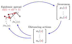
Figure 1: (a) Node-level state transition diagram. (b) System-level diagram

II-B Awareness SIS Model

We modify the benchmark model to take into account the agents’ awareness of the current epidemic state. The information agent i𝑖i receives comes from two sources: the proportion of infected neighbors in its local social network and a global broadcast of the proportion of infected nodes in the entire network. The social network is a graph 𝒢I=(𝒩,I)subscript𝒢𝐼𝒩subscript𝐼\mathcal{G}_{I}=(\mathcal{N},\mathcal{E}_{I}) with the same nodes as 𝒢Csubscript𝒢𝐶\mathcal{G}_{C} but with different edges, representing the nodes’ social communication links. The set of i𝑖i’s neighbors in 𝒢Isubscript𝒢𝐼\mathcal{G}_{I} is written 𝒩iIsuperscriptsubscript𝒩𝑖𝐼\mathcal{N}_{i}^{I}. The information is given by

μi(s)α|𝒩iI|j𝒩iIsj+1αnj=1nsj,sΩformulae-sequencesubscript𝜇𝑖𝑠𝛼superscriptsubscript𝒩𝑖𝐼subscript𝑗superscriptsubscript𝒩𝑖𝐼subscript𝑠𝑗1𝛼𝑛superscriptsubscript𝑗1𝑛subscript𝑠𝑗for-all𝑠Ω\mu_{i}(s)\triangleq\frac{\alpha}{|\mathcal{N}_{i}^{I}|}\sum_{j\in\mathcal{N}_{i}^{I}}s_{j}+\frac{1-\alpha}{n}\sum_{j=1}^{n}s_{j}\ ,\forall s\in\Omega (6)

where α[0,1]𝛼01\alpha\in[0,1] is a parameter that governs the trust nodes place in information from their social contacts. Consequently, node i𝑖i reduces its interactions with its physical neighbors through the social distancing action

ai(s)1μi(s),subscript𝑎𝑖𝑠1subscript𝜇𝑖𝑠a_{i}(s)\triangleq 1-\mu_{i}(s), (7)

which reduces its susceptible-to-infected probability (2) to

p01,di(s)1j𝒩iC(1βai(s)sj).superscriptsubscript𝑝01𝑑𝑖𝑠1subscriptproduct𝑗superscriptsubscript𝒩𝑖𝐶1𝛽subscript𝑎𝑖𝑠subscript𝑠𝑗p_{01,d}^{i}(s)\triangleq 1-\prod_{j\in\mathcal{N}_{i}^{C}}(1-\beta a_{i}(s)s_{j}). (8)

We similarly define p00,di(s)1p01,di(s)superscriptsubscript𝑝00𝑑𝑖𝑠1superscriptsubscript𝑝01𝑑𝑖𝑠p_{00,d}^{i}(s)\triangleq 1-p_{01,d}^{i}(s). An infected agent’s probability of recovering becomes δp00,di(s)𝛿superscriptsubscript𝑝00𝑑𝑖𝑠\delta p_{00,d}^{i}(s). Note for all sΩ𝑠Ωs\in\Omega, p01,di(s)p01i(s)superscriptsubscript𝑝01𝑑𝑖𝑠superscriptsubscript𝑝01𝑖𝑠p_{01,d}^{i}(s)\leq p_{01}^{i}(s). Combined with the social distancing behaviors aisubscript𝑎𝑖a_{i}, the local awareness spread dynamics in (6) make the effect of user behavior on its infection probability endogenous to the benchmark chain model through a negative feedback loop. We define the idsuperscriptsubscript𝑖𝑑\mathbb{P}_{i}^{d} analogously to (3) and (4):

IfsiIfsubscript𝑠𝑖\displaystyle\text{If}\ s_{i} =0,{id(s,0)=p00,di(s)id(s,1)=p01,di(s)absent0casessuperscriptsubscript𝑖𝑑𝑠0absentsuperscriptsubscript𝑝00𝑑𝑖𝑠superscriptsubscript𝑖𝑑𝑠1absentsuperscriptsubscript𝑝01𝑑𝑖𝑠\displaystyle=0,\begin{cases}\mathbb{P}_{i}^{d}(s,0)&=p_{00,d}^{i}(s)\\ \mathbb{P}_{i}^{d}(s,1)&=p_{01,d}^{i}(s)\end{cases} (9)
IfsiIfsubscript𝑠𝑖\displaystyle\text{If}\ s_{i} =1,{id(s,0)=δp00,di(s)id(s,1)=1δp00,di(s)absent1casessuperscriptsubscript𝑖𝑑𝑠0absent𝛿superscriptsubscript𝑝00𝑑𝑖𝑠superscriptsubscript𝑖𝑑𝑠1absent1𝛿superscriptsubscript𝑝00𝑑𝑖𝑠\displaystyle=1,\begin{cases}\mathbb{P}_{i}^{d}(s,0)&=\delta p_{00,d}^{i}(s)\\ \mathbb{P}_{i}^{d}(s,1)&=1-\delta p_{00,d}^{i}(s)\end{cases} (10)

Thus, the idsuperscriptsubscript𝑖𝑑\mathbb{P}_{i}^{d} define the distancing Markov chain over ΩΩ\Omega by the transition matrix Kdsubscript𝐾𝑑K_{d} with elements

Kd(s,s)i=1nid(s,si),s,sΩformulae-sequencesubscript𝐾𝑑𝑠superscript𝑠superscriptsubscriptproduct𝑖1𝑛superscriptsubscript𝑖𝑑𝑠superscriptsubscript𝑠𝑖for-all𝑠superscript𝑠ΩK_{d}(s,s^{\prime})\triangleq\prod_{i=1}^{n}\mathbb{P}_{i}^{d}(s,s_{i}^{\prime}),\ \forall s,s^{\prime}\in\Omega (11)

whose unique absorbing state is also 𝕠𝕠\mathbb{o}, the all-susceptible state. The feedback between social distancing actions and epidemic states is illustrated in Figure 1(b).

Remark 1.

Our model of awareness captures the different ways an agent may receive information about an ongoing epidemic from the media. Large media corporations and public health institutions such as the Centers for Disease Control and Prevention (CDC) and the World Health Organization (WHO) often report an estimated total number of people infected nationwide or globally at a given time, and this information is disseminated amongst the population. Information is also exchanged through one’s personalized social links, which can range beyond a person’s geographic location. Thus, a node’s awareness is composed of a linear combination of both sources of information, as given in (6).

III Mean-field Approximations

III-A Derivation

We derive a mean-field approximation (MFA) of the Markovian dynamics described in the previous section. The MFA is a deterministic, discrete-time dynamic system with an n𝑛n-dimensional state space [0,1]nsuperscript01𝑛[0,1]^{n}, which is interpreted to be each node’s probability of being infected at any given time.

Here, we write stΩsuperscript𝑠𝑡Ωs^{t}\in\Omega as the epidemic state at time t=0,1,𝑡01t=0,1,\ldots. Indeed, consider the node-level stochastic state transition update

sit+1=sitB(1δp00,di(st))+(1sit)B(p01,di(st))superscriptsubscript𝑠𝑖𝑡1superscriptsubscript𝑠𝑖𝑡𝐵1𝛿superscriptsubscript𝑝00𝑑𝑖superscript𝑠𝑡1superscriptsubscript𝑠𝑖𝑡𝐵superscriptsubscript𝑝01𝑑𝑖superscript𝑠𝑡s_{i}^{t+1}=s_{i}^{t}B(1-\delta p_{00,d}^{i}(s^{t}))+(1-s_{i}^{t})B(p_{01,d}^{i}(s^{t})) (12)

of the distancing chain where B(λ)𝐵𝜆B(\lambda) denotes a Bernoulli random variable with parameter λ[0,1]𝜆01\lambda\in[0,1]. For shorthand, we write xitPr(sit=1)superscriptsubscript𝑥𝑖𝑡Prsuperscriptsubscript𝑠𝑖𝑡1x_{i}^{t}\triangleq\text{Pr}(s_{i}^{t}=1) for the probability node i𝑖i is infected at time t𝑡t. Taking the probability of both sides equaling one,

xit+1superscriptsubscript𝑥𝑖𝑡1\displaystyle x_{i}^{t+1} =Pr(B(1δp00,di(st))=1|sit=1)Pr(sit=1)+absentPr𝐵1𝛿superscriptsubscript𝑝00𝑑𝑖superscript𝑠𝑡conditional1superscriptsubscript𝑠𝑖𝑡1Prsuperscriptsubscript𝑠𝑖𝑡1\displaystyle=\text{Pr}(B(1-\delta p_{00,d}^{i}(s^{t}))=1|s_{i}^{t}=1)\text{Pr}(s_{i}^{t}=1)+\cdots
Pr(B(p01,di(st))=1|sit=0)Pr(sit=0)Pr𝐵superscriptsubscript𝑝01𝑑𝑖superscript𝑠𝑡conditional1superscriptsubscript𝑠𝑖𝑡0Prsuperscriptsubscript𝑠𝑖𝑡0\displaystyle\ \ \ \ \text{Pr}(B(p_{01,d}^{i}(s^{t}))=1|s_{i}^{t}=0)\text{Pr}(s_{i}^{t}=0)
=xit(1δp00,di(st))+(1xit)p01,di(st)absentsuperscriptsubscript𝑥𝑖𝑡1𝛿superscriptsubscript𝑝00𝑑𝑖superscript𝑠𝑡1superscriptsubscript𝑥𝑖𝑡superscriptsubscript𝑝01𝑑𝑖superscript𝑠𝑡\displaystyle=x_{i}^{t}(1-\delta p_{00,d}^{i}(s^{t}))+(1-x_{i}^{t})p_{01,d}^{i}(s^{t})
=xit(1δ)+(1(1δ)xit)p01,di(st)absentsuperscriptsubscript𝑥𝑖𝑡1𝛿11𝛿superscriptsubscript𝑥𝑖𝑡superscriptsubscript𝑝01𝑑𝑖superscript𝑠𝑡\displaystyle=x_{i}^{t}(1-\delta)+(1-(1-\delta)x_{i}^{t})p_{01,d}^{i}(s^{t}) (13)

Note the expression for xit+1superscriptsubscript𝑥𝑖𝑡1x_{i}^{t+1} still depends stochastically on the state stsuperscript𝑠𝑡s^{t}. To obtain a mean-field approximation of xit+1superscriptsubscript𝑥𝑖𝑡1x_{i}^{t+1}, we simply replace the state stsuperscript𝑠𝑡s^{t} with xtsuperscript𝑥𝑡x^{t} (the n𝑛n-vector with components xitsuperscriptsubscript𝑥𝑖𝑡x_{i}^{t}) in (III-A). Thus, by redefining xit+1superscriptsubscript𝑥𝑖𝑡1x_{i}^{t+1} to obey this approximation and extending the domain of μi(),ai()subscript𝜇𝑖subscript𝑎𝑖\mu_{i}(\cdot),a_{i}(\cdot) and p01,di()superscriptsubscript𝑝01𝑑𝑖p_{01,d}^{i}(\cdot) from {0,1}nsuperscript01𝑛\{0,1\}^{n} to [0,1]nsuperscript01𝑛[0,1]^{n}, we have the following approximate dynamics

xit+1=xit(1δ)+(1(1δ)xit)p01,di(xt)superscriptsubscript𝑥𝑖𝑡1superscriptsubscript𝑥𝑖𝑡1𝛿11𝛿superscriptsubscript𝑥𝑖𝑡superscriptsubscript𝑝01𝑑𝑖superscript𝑥𝑡x_{i}^{t+1}=x_{i}^{t}(1-\delta)+(1-(1-\delta)x_{i}^{t})p_{01,d}^{i}(x^{t}) (14)

on the time evolution of node i𝑖i’s probability of being infected. Stacking the dynamics for each node into a vector, we obtain a mapping ϕ:[0,1]n[0,1]n:italic-ϕsuperscript01𝑛superscript01𝑛\phi:[0,1]^{n}\rightarrow[0,1]^{n} where ϕi(x)=xi(1δ)+(1(1δ)xi)p01,di(x)subscriptitalic-ϕ𝑖𝑥subscript𝑥𝑖1𝛿11𝛿subscript𝑥𝑖superscriptsubscript𝑝01𝑑𝑖𝑥\phi_{i}(x)=x_{i}(1-\delta)+(1-(1-\delta)x_{i})p_{01,d}^{i}(x) and xt+1=ϕ(xt)superscript𝑥𝑡1italic-ϕsuperscript𝑥𝑡x^{t+1}=\phi(x^{t}). This MFA of the distancing chain is in contrast to the MFA of the benchmark chain,

xit+1=xit(1δ)+(1(1δ)xit)p01i(xt)superscriptsubscript𝑥𝑖𝑡1superscriptsubscript𝑥𝑖𝑡1𝛿11𝛿superscriptsubscript𝑥𝑖𝑡superscriptsubscript𝑝01𝑖superscript𝑥𝑡x_{i}^{t+1}=x_{i}^{t}(1-\delta)+(1-(1-\delta)x_{i}^{t})p_{01}^{i}(x^{t}) (15)

which is studied thoroughly in [6]. It is derived in the same manner, and is described by the mapping ψ:[0,1]n[0,1]n:𝜓superscript01𝑛superscript01𝑛\psi:[0,1]^{n}\rightarrow[0,1]^{n} with ψi(x)=xi(1δ)+(1(1δ)xi)p01i(x)subscript𝜓𝑖𝑥subscript𝑥𝑖1𝛿11𝛿subscript𝑥𝑖superscriptsubscript𝑝01𝑖𝑥\psi_{i}(x)=x_{i}(1-\delta)+(1-(1-\delta)x_{i})p_{01}^{i}(x) and xt+1=ψ(xt)superscript𝑥𝑡1𝜓superscript𝑥𝑡x^{t+1}=\psi(x^{t}).

We make a few remarks on the basic structure of these two mappings. They are nonlinear, continuous mappings satisfying ϕ(x)ψ(x)precedesitalic-ϕ𝑥𝜓𝑥\phi(x)\prec\psi(x) whenever x[0,1]n\𝟘n𝑥\superscript01𝑛subscript0𝑛x\in[0,1]^{n}\backslash\mathbb{0}_{n} and α[0,1)𝛼01\alpha\in[0,1). Also, ϕ(𝟘n)=ψ(𝟘n)=𝟘nitalic-ϕsubscript0𝑛𝜓subscript0𝑛subscript0𝑛\phi(\mathbb{0}_{n})=\psi(\mathbb{0}_{n})=\mathbb{0}_{n}. Linearization of ϕitalic-ϕ\phi and ψ𝜓\psi about the origin yields the same Jacobian matrix, βAC+(1δ)I𝛽subscript𝐴𝐶1𝛿𝐼\beta A_{C}+(1-\delta)I, and hence the same linearized dynamics xt+1=(βAC+(1δ)I)xtsuperscript𝑥𝑡1𝛽subscript𝐴𝐶1𝛿𝐼superscript𝑥𝑡x^{t+1}=(\beta A_{C}+(1-\delta)I)x^{t}. The linear dynamics serve as an upper bound to both (14) and (15). Therefore, if λmax(βAC+(1δ)I)<1subscript𝜆max𝛽subscript𝐴𝐶1𝛿𝐼1\lambda_{\text{max}}(\beta A_{C}+(1-\delta)I)<1, the origin is a globally stable fixed point and it is an unstable fixed point if λmax(βAC+(1δ)I)>1subscript𝜆max𝛽subscript𝐴𝐶1𝛿𝐼1\lambda_{\text{max}}(\beta A_{C}+(1-\delta)I)>1.

III-B Existence of a Non-trivial Fixed Point

We now provide a sufficient condition for the existence of a non-trivial fixed point (𝟘nsucceedsabsentsubscript0𝑛\succ\mathbb{0}_{n}, the n𝑛n-vector of zeros) of ϕitalic-ϕ\phi.

Theorem 1.

If λmax(βAC+(1δ)In)>1subscript𝜆max𝛽subscript𝐴𝐶1𝛿subscript𝐼𝑛1\lambda_{\text{max}}(\beta A_{C}+(1-\delta)I_{n})>1, there exists a nontrivial fixed point for ϕitalic-ϕ\phi.

The existence of such a fixed point suggests the epidemic has an endemic state, where the disease spreads fast enough to sustain an epidemic in the network. Our condition coincides with the condition for existence, uniqueness, and global asymptotic stability of the non-trivial fixed point qsuperscript𝑞q^{*} of ψ𝜓\psi, which is λmax(βAC+(1δ)I)>1subscript𝜆max𝛽subscript𝐴𝐶1𝛿𝐼1\lambda_{\text{max}}(\beta A_{C}+(1-\delta)I)>1, i.e. when the origin in the linearized dynamics is unstable (Theorem 5.1, [6]). This condition incorporates the factors that contribute to the rate of spreading - δ,β𝛿𝛽\delta,\beta, and the contact network ACsubscript𝐴𝐶A_{C}. The proof makes use of the following lemmas.

Lemma 1 (Lemma 3.1, [6]).

There exists a vector ν0nsucceeds𝜈subscript0𝑛\nu\succ 0_{n} such that (βACδIn)ν0nsucceeds𝛽subscript𝐴𝐶𝛿subscript𝐼𝑛𝜈subscript0𝑛(\beta A_{C}-\delta I_{n})\nu\succ 0_{n} if and only if λmax(βAC+(1δ)In)>1subscript𝜆max𝛽subscript𝐴𝐶1𝛿subscript𝐼𝑛1\lambda_{\text{max}}(\beta A_{C}+(1-\delta)I_{n})>1.

The connectedness assumption for 𝒢Csubscript𝒢𝐶\mathcal{G}_{C} is necessary for the above Lemma because the proof applies the Perron-Frobenius theorem for nonnegative irreducible matrices. The next result is an equivalent formulation of Brouwer’s fixed point theorem.

Lemma 2.

(Theorem 4.2.3, [31]): Suppose fi:Dn,i=1,,n:subscript𝑓𝑖formulae-sequencesubscript𝐷𝑛𝑖1𝑛f_{i}:D_{n}\rightarrow\mathbb{R},i=1,\ldots,n are continuous mappings, where

Dn={xn:xi[i,ui],i}subscript𝐷𝑛conditional-set𝑥superscript𝑛subscript𝑥𝑖subscript𝑖subscript𝑢𝑖for-all𝑖D_{n}=\{x\in\mathbb{R}^{n}:x_{i}\in[\ell_{i},u_{i}],\ \forall i\}

for real numbers i,uisubscript𝑖subscript𝑢𝑖\ell_{i},u_{i}. We also define the set

Di={xin1:xj[j,uj]ji}subscript𝐷𝑖conditional-setsubscript𝑥𝑖superscript𝑛1subscript𝑥𝑗subscript𝑗subscript𝑢𝑗for-all𝑗𝑖D_{-i}=\{x_{-i}\in\mathbb{R}^{n-1}:x_{j}\in[\ell_{j},u_{j}]\ \forall j\neq i\}

If for every i𝑖i and for all xiDisubscript𝑥𝑖subscript𝐷𝑖x_{-i}\in D_{-i},

fi(x1,,i,,xn)subscript𝑓𝑖subscript𝑥1subscript𝑖subscript𝑥𝑛\displaystyle f_{i}(x_{1},\ldots,\ell_{i},\ldots,x_{n}) =fi(xi,i)0absentsubscript𝑓𝑖subscript𝑥𝑖subscript𝑖0\displaystyle=f_{i}(x_{-i},\ell_{i})\geq 0 (16)
fi(x1,,ui,,xn)subscript𝑓𝑖subscript𝑥1subscript𝑢𝑖subscript𝑥𝑛\displaystyle f_{i}(x_{1},\ldots,u_{i},\ldots,x_{n}) =fi(xi,ui)0,absentsubscript𝑓𝑖subscript𝑥𝑖subscript𝑢𝑖0\displaystyle=f_{i}(x_{-i},u_{i})\leq 0, (17)

then there exists a point xDnsuperscript𝑥subscript𝐷𝑛x^{*}\in D_{n} such that fi(x)=0subscript𝑓𝑖superscript𝑥0f_{i}(x^{*})=0, for all i=1,,n𝑖1𝑛i=1,\ldots,n.

The final lemma needed is a technical result for the mean-field mappings ϕisubscriptitalic-ϕ𝑖\phi_{i}.

Lemma 3.

For each i𝒩𝑖𝒩i\in\mathcal{N}, define the maps fi:[0,1]n:subscript𝑓𝑖superscript01𝑛f_{i}:[0,1]^{n}\rightarrow\mathbb{R}

fi(x)subscript𝑓𝑖𝑥\displaystyle f_{i}(x) ϕi(x)xiabsentsubscriptitalic-ϕ𝑖𝑥subscript𝑥𝑖\displaystyle\triangleq\phi_{i}(x)-x_{i}
=δxi+(1(1δ)xi)p01,di(x)absent𝛿subscript𝑥𝑖11𝛿subscript𝑥𝑖superscriptsubscript𝑝01𝑑𝑖𝑥\displaystyle=-\delta x_{i}+(1-(1-\delta)x_{i})p_{01,d}^{i}(x) (18)

Then for any i𝒩𝑖𝒩i\in\mathcal{N} and xi[0,1]n1subscript𝑥𝑖superscript01𝑛1x_{-i}\in[0,1]^{n-1}, the function fi(xi,)subscript𝑓𝑖subscript𝑥𝑖f_{i}(x_{-i},\cdot) has a unique root ci(xi)[0,1)superscriptsubscript𝑐𝑖subscript𝑥𝑖01c_{i}^{*}(x_{-i})\in[0,1) which depends continuously on xisubscript𝑥𝑖x_{-i}. Furthermore, one can find a sequence xik𝟘n1superscriptsubscript𝑥𝑖𝑘subscript0𝑛1x_{-i}^{k}\rightarrow\mathbb{0}_{n-1} s.t. ci(xik)superscriptsubscript𝑐𝑖superscriptsubscript𝑥𝑖𝑘c_{i}^{*}(x_{-i}^{k}) is monotonically decreasing to 0.

Proof.

For any i𝒩𝑖𝒩i\in\mathcal{N} and xi[0,1]n1subscript𝑥𝑖superscript01𝑛1x_{-i}\in[0,1]^{n-1},

fi(xi,0)=p01,di(xi,0)0.subscript𝑓𝑖subscript𝑥𝑖0superscriptsubscript𝑝01𝑑𝑖subscript𝑥𝑖00f_{i}(x_{-i},0)=p_{01,d}^{i}(x_{-i},0)\geq 0. (19)

and

fi(xi,1)=δ(p01,di(xi,1)1)<0.subscript𝑓𝑖subscript𝑥𝑖1𝛿superscriptsubscript𝑝01𝑑𝑖subscript𝑥𝑖110f_{i}(x_{-i},1)=\delta(p_{01,d}^{i}(x_{-i},1)-1)<0. (20)

The function fi(xi,)subscript𝑓𝑖subscript𝑥𝑖f_{i}(x_{-i},\cdot) is strictly decreasing: for a,b[0,1]𝑎𝑏01a,b\in[0,1] s.t. a<b𝑎𝑏a<b, fi(xi,a)fi(xi,b)subscript𝑓𝑖subscript𝑥𝑖𝑎subscript𝑓𝑖subscript𝑥𝑖𝑏f_{i}(x_{-i},a)-f_{i}(x_{-i},b) is given by

(ba)𝑏𝑎\displaystyle(b-a) (δ+(1δ)p01,di(xi,b))+𝛿1𝛿superscriptsubscript𝑝01𝑑𝑖subscript𝑥𝑖𝑏\displaystyle(\delta+(1-\delta)p_{01,d}^{i}(x_{-i},b))+\cdots
+(1a(1δ))(p01,di(xi,a)p01,di(xi,b))1𝑎1𝛿superscriptsubscript𝑝01𝑑𝑖subscript𝑥𝑖𝑎superscriptsubscript𝑝01𝑑𝑖subscript𝑥𝑖𝑏\displaystyle+(1-a(1-\delta))(p_{01,d}^{i}(x_{-i},a)-p_{01,d}^{i}(x_{-i},b))
>0.absent0\displaystyle>0.

This follows because p01,di(xi,xi)superscriptsubscript𝑝01𝑑𝑖subscript𝑥𝑖subscript𝑥𝑖p_{01,d}^{i}(x_{-i},x_{i}) is decreasing in xisubscript𝑥𝑖x_{i} (xisubscript𝑥𝑖x_{i} contributes to global awareness). Hence for every xi[0,1]n1subscript𝑥𝑖superscript01𝑛1x_{-i}\in[0,1]^{n-1}, there is a unique ci(xi)[0,1)superscriptsubscript𝑐𝑖subscript𝑥𝑖01c_{i}^{*}(x_{-i})\in[0,1) s.t. fi(xi,ci(xi))=0subscript𝑓𝑖subscript𝑥𝑖superscriptsubscript𝑐𝑖subscript𝑥𝑖0f_{i}(x_{-i},c_{i}^{*}(x_{-i}))=0, and ci(xi)superscriptsubscript𝑐𝑖subscript𝑥𝑖c_{i}^{*}(x_{-i}) depends continuously on xisubscript𝑥𝑖x_{-i}. To see this, observe that ci(xi)[0,1)superscriptsubscript𝑐𝑖subscript𝑥𝑖01c_{i}^{*}(x_{-i})\in[0,1) is a root of the equation

(1(1δ)xi)(1j𝒩iC(1ai(xi,xi)βxj))δxi=0,11𝛿subscript𝑥𝑖1subscriptproduct𝑗superscriptsubscript𝒩𝑖𝐶1subscript𝑎𝑖subscript𝑥𝑖subscript𝑥𝑖𝛽subscript𝑥𝑗𝛿subscript𝑥𝑖0(1-(1-\delta)x_{i})\left(1-\prod_{j\in\mathcal{N}_{i}^{C}}(1-a_{i}(x_{-i},x_{i})\beta x_{j})\right)-\delta x_{i}=0, (21)

which is a polynomial in xisubscript𝑥𝑖x_{i}. The coefficients of the polynomial depend continuously on xi[0,1]n1subscript𝑥𝑖superscript01𝑛1x_{-i}\in[0,1]^{n-1}, and the roots of any polynomial are continuous with respect to its coefficients. Consequently, for any sequence xik𝟘n1superscriptsubscript𝑥𝑖𝑘subscript0𝑛1x_{-i}^{k}\rightarrow\mathbb{0}_{n-1}, ci(xik)ci(𝟘n1)=0superscriptsubscript𝑐𝑖superscriptsubscript𝑥𝑖𝑘superscriptsubscript𝑐𝑖subscript0𝑛10c_{i}^{*}(x_{-i}^{k})\rightarrow c_{i}^{*}(\mathbb{0}_{n-1})=0 by continuity. This allows us to select a subsequence of xiksuperscriptsubscript𝑥𝑖𝑘x_{-i}^{k} such that cisuperscriptsubscript𝑐𝑖c_{i}^{*} is monotonically decreasing along the subsequence. ∎

We are now ready to prove the main result of this section.

Proof of Theorem 1:.

Let the mappings fisubscript𝑓𝑖f_{i}, i𝒩𝑖𝒩i\in\mathcal{N} be as in Lemma 3. We need to verify (16) and (17) hold for all i𝑖i and for choices of i,uisubscript𝑖subscript𝑢𝑖\ell_{i},u_{i} satisfying 0<i<ui0subscript𝑖subscript𝑢𝑖0<\ell_{i}<u_{i}. This ensures the awareness dynamic ϕitalic-ϕ\phi has a fixed point other than the origin.
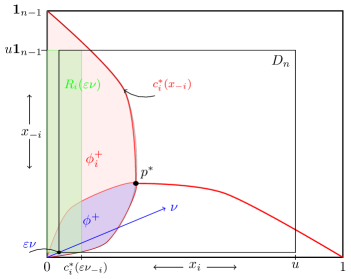
Refer to caption
Figure 2: Diagram of the proof of Theorem 1. Here, psuperscript𝑝p^{*} denotes a nontrivial fixed point of ϕitalic-ϕ\phi.

Choose ui=usubscript𝑢𝑖𝑢u_{i}=u where u𝑢u satisfies

maxi𝒩maxxi[0,1]n1ci(xi)<u<1.subscript𝑖𝒩subscriptsubscript𝑥𝑖superscript01𝑛1superscriptsubscript𝑐𝑖subscript𝑥𝑖𝑢1\max_{i\in\mathcal{N}}\max_{x_{-i}\in[0,1]^{n-1}}c_{i}^{*}(x_{-i})<u<1. (22)

Then for all xi[0,u]n1subscript𝑥𝑖superscript0𝑢𝑛1x_{-i}\in[0,u]^{n-1},

fi(xi,u)<0subscript𝑓𝑖subscript𝑥𝑖𝑢0f_{i}(x_{-i},u)<0 (23)

since u>ci(xi)𝑢superscriptsubscript𝑐𝑖subscript𝑥𝑖u>c_{i}^{*}(x_{-i}). Thus, (17) holds, regardless of the choice of isubscript𝑖\ell_{i}. However, it remains to find the i>0subscript𝑖0\ell_{i}>0 s.t. (16) is satisfied. Let f(x)[f1(x),,fn(x)]T𝑓𝑥superscriptsubscript𝑓1𝑥subscript𝑓𝑛𝑥𝑇f(x)\triangleq[f_{1}(x),\ldots,f_{n}(x)]^{T} and define the sets

ϕi+{x[0,1]n:fi(x)0},ϕ+j=1nϕj+formulae-sequencesubscriptsuperscriptitalic-ϕ𝑖conditional-set𝑥superscript01𝑛subscript𝑓𝑖𝑥0superscriptitalic-ϕsuperscriptsubscript𝑗1𝑛superscriptsubscriptitalic-ϕ𝑗\phi^{+}_{i}\triangleq\{x\in[0,1]^{n}:f_{i}(x)\geq 0\},\ \ \phi^{+}\triangleq\bigcap_{j=1}^{n}\phi_{j}^{+} (24)

The Jacobian of f𝑓f about the origin is (βACδIn)𝛽subscript𝐴𝐶𝛿subscript𝐼𝑛(\beta A_{C}-\delta I_{n}). By Lemma 1, there exists a vector ν𝟘nsucceeds𝜈subscript0𝑛\nu\succ\mathbb{0}_{n} such that (βACδIn)ν𝟘nsucceeds𝛽subscript𝐴𝐶𝛿subscript𝐼𝑛𝜈subscript0𝑛(\beta A_{C}-\delta I_{n})\nu\succ\mathbb{0}_{n}. Consequently for sufficiently small ε>0𝜀0\varepsilon>0,

f(εν)𝟘n,succeeds𝑓𝜀𝜈subscript0𝑛f(\varepsilon\nu)\succ\mathbb{0}_{n}, (25)

or ενϕ+𝜀𝜈superscriptitalic-ϕ\varepsilon\nu\in\phi^{+}. We also define the set

Ri(xi){yn:yi[0,ci(xi)],yj[xj,u],ji}subscript𝑅𝑖subscript𝑥𝑖conditional-set𝑦superscript𝑛formulae-sequencesubscript𝑦𝑖0superscriptsubscript𝑐𝑖subscript𝑥𝑖formulae-sequencesubscript𝑦𝑗subscript𝑥𝑗𝑢𝑗𝑖R_{i}(x_{-i})\triangleq\{y\in\mathbb{R}^{n}:y_{i}\in[0,c_{i}^{*}(x_{-i})],y_{j}\in[x_{j},u],j\neq i\} (26)

If ενici(ενi)𝜀subscript𝜈𝑖superscriptsubscript𝑐𝑖𝜀subscript𝜈𝑖\varepsilon\nu_{i}\leq c_{i}^{*}(\varepsilon\nu_{-i}) and Ri(εν)ϕi+subscript𝑅𝑖𝜀𝜈superscriptsubscriptitalic-ϕ𝑖R_{i}(\varepsilon\nu)\subset\phi_{i}^{+}, then (16) is satisfied, i.e. fi(xi,ενi)0subscript𝑓𝑖subscript𝑥𝑖𝜀subscript𝜈𝑖0f_{i}(x_{-i},\varepsilon\nu_{i})\geq 0 on Di={ενixiu𝟙n1}subscript𝐷𝑖precedes-or-equals𝜀subscript𝜈𝑖subscript𝑥𝑖precedes-or-equals𝑢subscript1𝑛1D_{-i}=\{\varepsilon\nu_{-i}\preceq x_{-i}\preceq u\mathbb{1}_{n-1}\} for ε𝜀\varepsilon sufficiently small. We already have ενici(ενi)𝜀subscript𝜈𝑖superscriptsubscript𝑐𝑖𝜀subscript𝜈𝑖\varepsilon\nu_{i}\leq c_{i}^{*}(\varepsilon\nu_{-i}) because ενϕ+ϕi+𝜀𝜈superscriptitalic-ϕsuperscriptsubscriptitalic-ϕ𝑖\varepsilon\nu\in\phi^{+}\subset\phi_{i}^{+}. To show Ri(εν)ϕi+subscript𝑅𝑖𝜀𝜈superscriptsubscriptitalic-ϕ𝑖R_{i}(\varepsilon\nu)\subset\phi_{i}^{+}, by Lemma 3 we can find a sequence εkνϕ+subscript𝜀𝑘𝜈superscriptitalic-ϕ\varepsilon_{k}\nu\in\phi^{+} with εk0subscript𝜀𝑘0\varepsilon_{k}\rightarrow 0 s.t. ci(εkνi)superscriptsubscript𝑐𝑖subscript𝜀𝑘subscript𝜈𝑖c_{i}^{*}(\varepsilon_{k}\nu_{-i}) is monotonically decreasing to 0. By stopping at a large enough k𝑘k, we can take a ε𝜀\varepsilon small enough such that

ci(ενi)=minxiDici(xi)superscriptsubscript𝑐𝑖𝜀subscript𝜈𝑖subscriptsubscript𝑥𝑖subscript𝐷𝑖superscriptsubscript𝑐𝑖subscript𝑥𝑖c_{i}^{*}(\varepsilon\nu_{-i})=\min_{x_{-i}\in D_{-i}}c_{i}^{*}(x_{-i}) (27)

Consequently, Ri(εν)ϕi+subscript𝑅𝑖𝜀𝜈superscriptsubscriptitalic-ϕ𝑖R_{i}(\varepsilon\nu)\subset\phi_{i}^{+}. Choosing ε𝜀\varepsilon small enough to satisfy (27) for all i𝒩𝑖𝒩i\in\mathcal{N} verifies (16) by using Dn={xn:xj[ενj,u]}subscript𝐷𝑛conditional-set𝑥superscript𝑛subscript𝑥𝑗𝜀subscript𝜈𝑗𝑢D_{n}=\{x\in\mathbb{R}^{n}:x_{j}\in[\varepsilon\nu_{j},u]\}. See Figure 2 for an illustration of the proof. By Lemma 2, ϕitalic-ϕ\phi has a fixed point contained in Dnsubscript𝐷𝑛D_{n}. ∎

The condition of Theorem 1 is independent of the awareness parameter α𝛼\alpha and the structure of the information network 𝒢Isubscript𝒢𝐼\mathcal{G}_{I}. Hence, social distancing alone cannot restore stability of the disease-free equilibrium point. However, social distancing lowers the overall metastable state of an epidemic.

Corollary 1.

If q𝟘nsucceedssuperscript𝑞subscript0𝑛q^{*}\succ\mathbb{0}_{n} is the unique nontrivial fixed point of ψ𝜓\psi, then any nontrivial fixed point psuperscript𝑝p^{*} of ϕitalic-ϕ\phi satisfies pqprecedessuperscript𝑝superscript𝑞p^{*}\prec q^{*} whenever α[0,1)𝛼01\alpha\in[0,1).

Proof.

Define the sets ψi+superscriptsubscript𝜓𝑖\psi_{i}^{+} and ψ+superscript𝜓\psi^{+} similarly as in (24). It was shown in [6] that qsuperscript𝑞q^{*} is the unique maximal element of ψ+superscript𝜓\psi^{+}, i.e qqsucceedssuperscript𝑞𝑞q^{*}\succ q, qψ+for-all𝑞superscript𝜓\forall q\in\psi^{+}, qq𝑞superscript𝑞q\neq q^{*}. Observe ϕ(x)ψ(x)precedesitalic-ϕ𝑥𝜓𝑥\phi(x)\prec\psi(x) for any x[0,1]n\𝟘n𝑥\superscript01𝑛subscript0𝑛x\in[0,1]^{n}\backslash\mathbb{0}_{n}. Let xϕ+𝑥superscriptitalic-ϕx\in\phi^{+}, x𝟘n𝑥subscript0𝑛x\neq\mathbb{0}_{n}. Then xϕ(x)ψ(x)precedes-or-equals𝑥italic-ϕ𝑥precedes𝜓𝑥x\preceq\phi(x)\prec\psi(x), so xψ+𝑥superscript𝜓x\in\psi^{+}. Therefore, ϕ+ψ+superscriptitalic-ϕsuperscript𝜓\phi^{+}\subset\psi^{+}, and since pϕ+superscript𝑝superscriptitalic-ϕp^{*}\in\phi^{+} for any nontrivial fixed point of ϕitalic-ϕ\phi, pqprecedessuperscript𝑝superscript𝑞p^{*}\prec q^{*}. ∎

The mean-field analysis of this section reveals the qualitative dynamics not addressed by an absorbing Markov chain analysis. Since the all-susceptible state is the unique absorbing state and accessible from every other state, the disease eradicates in finite time with probability one. This answers what happens in the long-run, whereas the MFA analysis answers what happens before this eventuality. The MFA analysis concurs with what is observed in simulations of the Markov chain dynamics - fast convergence to an endemic “metastable” state that persists for a very long time before eradication. Numerical simulations suggest stability of one particular nontrivial fixed point psuperscript𝑝p^{*} of ϕitalic-ϕ\phi. A characterization of these fixed points for different random graph families is given in Section V.

IV Stochastic Comparison Between Awareness and Benchmark Model

In this section, we use the properties of monotone couplings to prove that adding awareness reduces the expectation of any increasing random variable quantifying an epidemic metric (e.g. absorption time, total infections), and that the benchmark chain dominates the distancing chain in terms of a partial ordering on sample paths. These results serve as a probabilistic analogue to the conclusions made in Section III about the strict ordering of the nontrivial fixed points in the corresponding mean-field approximations. Here, we have a closed form expression for the reduction whereas in Corollary 1, only an inequality relation is established. First, we provide relevant definitions and basic preliminary results of monotone couplings. For a full reference on monotone coupling, see Ch 4 of [32].

IV-A Monotone couplings

Consider a general countable space X𝑋X. Recall a partially ordered set (X,X)𝑋subscriptprecedes-or-equals𝑋(X,\preceq_{X}) is the set X𝑋X together with a relation Xsubscriptprecedes-or-equals𝑋\preceq_{X} among its elements which satisfies for all x,y𝑥𝑦x,y, and zX𝑧𝑋z\in X,

  • xXxsubscriptprecedes-or-equals𝑋𝑥𝑥x\preceq_{X}x

  • If xXysubscriptprecedes-or-equals𝑋𝑥𝑦x\preceq_{X}y and yXzsubscriptprecedes-or-equals𝑋𝑦𝑧y\preceq_{X}z, then xXzsubscriptprecedes-or-equals𝑋𝑥𝑧x\preceq_{X}z

  • If xXysubscriptprecedes-or-equals𝑋𝑥𝑦x\preceq_{X}y and yXxsubscriptprecedes-or-equals𝑋𝑦𝑥y\preceq_{X}x, then x=y𝑥𝑦x=y.

Definition 1.

Let p1,p2subscript𝑝1subscript𝑝2p_{1},p_{2} be probability measures on a measurable space (X,)𝑋(X,\mathcal{F}) and suppose (X,X)𝑋subscriptprecedes-or-equals𝑋(X,\preceq_{X}) is a partially ordered set. A monotone coupling of p1,p2subscript𝑝1subscript𝑝2p_{1},p_{2} is a probability measure p𝑝p on (X2,2)superscript𝑋2superscript2(X^{2},\mathcal{F}^{2}) such that for all x,yXsuperscript𝑥superscript𝑦𝑋x^{\prime},y^{\prime}\in X,

xXyp(x,y)=p2(y)andyXxp(x,y)=p1(x).subscriptsubscriptprecedes-or-equals𝑋𝑥superscript𝑦𝑝𝑥superscript𝑦subscript𝑝2superscript𝑦andsubscriptsubscriptsucceeds-or-equals𝑋𝑦superscript𝑥𝑝superscript𝑥𝑦subscript𝑝1superscript𝑥\sum_{x\preceq_{X}y^{\prime}}p(x,y^{\prime})=p_{2}(y^{\prime})\ \text{and}\ \sum_{y\succeq_{X}x^{\prime}}p(x^{\prime},y)=p_{1}(x^{\prime}). (28)

Thus, for any x,yX𝑥𝑦𝑋x,y\in X s.t xXysubscriptnot-precedes-or-equals𝑋𝑥𝑦x\not\preceq_{X}y, p(x,y)=0𝑝𝑥𝑦0p(x,y)=0, and the marginals of p𝑝p are p1,p2subscript𝑝1subscript𝑝2p_{1},p_{2}.

Example 1.

For an illustrative example of monotone coupling, consider two biased coins where the biases qA,qB<1subscript𝑞𝐴subscript𝑞𝐵1q_{A},q_{B}<1 for landing heads satisfy qA<qBsubscript𝑞𝐴subscript𝑞𝐵q_{A}<q_{B}. The coupling is a joint distribution assigned to the pair of coin flips to ensure the qAsubscript𝑞𝐴q_{A} coin can never land heads with the qBsubscript𝑞𝐵q_{B} coin landing tails, while the marginal coin flip probabilities remain the same. Specifically, define pX(0)=1qX,pX(1)=qXformulae-sequencesubscript𝑝𝑋01subscript𝑞𝑋subscript𝑝𝑋1subscript𝑞𝑋p_{X}(0)=1-q_{X},p_{X}(1)=q_{X} for X{A,B}𝑋𝐴𝐵X\in\{A,B\}. Also, define pAB:{0,1}2[0,1]:subscript𝑝𝐴𝐵superscript01201p_{AB}:\{0,1\}^{2}\rightarrow[0,1] by

{pAB(0,0)= 1qBpAB(0,1)=qBqApAB(1,0)= 0pAB(1,1)=qAcasessubscript𝑝𝐴𝐵00absent1subscript𝑞𝐵subscript𝑝𝐴𝐵01absentsubscript𝑞𝐵subscript𝑞𝐴subscript𝑝𝐴𝐵10absent 0subscript𝑝𝐴𝐵11absentsubscript𝑞𝐴\begin{cases}p_{AB}(0,0)&=\ 1-q_{B}\\ p_{AB}(0,1)&=\ q_{B}-q_{A}\\ p_{AB}(1,0)&=\ 0\\ p_{AB}(1,1)&=\ q_{A}\end{cases} (29)

Checking (28), the marginals are such that b1pAB(1,b)=qAsubscript𝑏1subscript𝑝𝐴𝐵1𝑏subscript𝑞𝐴\sum_{b\geq 1}p_{AB}(1,b)=q_{A}, a1pAB(a,1)=qBsubscript𝑎1subscript𝑝𝐴𝐵𝑎1subscript𝑞𝐵\sum_{a\leq 1}p_{AB}(a,1)=q_{B} and b0pAB(0,b)=1qAsubscript𝑏0subscript𝑝𝐴𝐵0𝑏1subscript𝑞𝐴\sum_{b\geq 0}p_{AB}(0,b)=1-q_{A}, a0pAB(a,0)=1qBsubscript𝑎0subscript𝑝𝐴𝐵𝑎01subscript𝑞𝐵\sum_{a\leq 0}p_{AB}(a,0)=1-q_{B} . Thus, pABsubscript𝑝𝐴𝐵p_{AB} is a monotone coupling of pA,pBsubscript𝑝𝐴subscript𝑝𝐵p_{A},p_{B}.

We say a function Z:X:𝑍𝑋Z:X\rightarrow\mathbb{R} is increasing in X𝑋X if whenever xXysubscriptprecedes-or-equals𝑋𝑥𝑦x\preceq_{X}y, Z(x)Z(y)𝑍𝑥𝑍𝑦Z(x)\leq Z(y). The next result characterizes the difference in expectations of increasing random variables between the marginals of a monotone coupling.

Proposition 1.

Keeping the notation of Definition 1, suppose p𝑝p is a monotone coupling of p1,p2subscript𝑝1subscript𝑝2p_{1},p_{2}. If a random variable Z:X+:𝑍𝑋subscriptZ:X\rightarrow\mathbb{Z}_{+} is increasing in X𝑋X, then

𝔼p2(Z)𝔼p1(Z)=τ=0p(Zτc,Zτ)subscript𝔼subscript𝑝2𝑍subscript𝔼subscript𝑝1𝑍superscriptsubscript𝜏0𝑝superscriptsubscript𝑍𝜏𝑐subscript𝑍𝜏\mathbb{E}_{p_{2}}(Z)-\mathbb{E}_{p_{1}}(Z)=\sum_{\tau=0}^{\infty}p(Z_{\tau}^{c},Z_{\tau}) (30)

where Zτ={x:Z(x)>τ}subscript𝑍𝜏conditional-set𝑥𝑍𝑥𝜏Z_{\tau}=\{x:Z(x)>\tau\}.

Proof.

Consider the following quantities:

p(Zτ,Zτ)𝑝subscript𝑍𝜏subscript𝑍𝜏\displaystyle p(Z_{\tau},Z_{\tau}) =xZτyZτp(x,y)absentsubscript𝑥subscript𝑍𝜏subscript𝑦subscript𝑍𝜏𝑝𝑥𝑦\displaystyle=\sum_{x\in Z_{\tau}}\sum_{y\in Z_{\tau}}p(x,y)
=xZτyXxp(x,y)=p1(Zτ)absentsubscript𝑥subscript𝑍𝜏subscriptsubscriptsucceeds-or-equals𝑋𝑦𝑥𝑝𝑥𝑦subscript𝑝1subscript𝑍𝜏\displaystyle=\sum_{x\in Z_{\tau}}\sum_{y\succeq_{X}x}p(x,y)=p_{1}(Z_{\tau}) (31)
p(X,Zτ)𝑝𝑋subscript𝑍𝜏\displaystyle p(X,Z_{\tau}) =p2(Zτ)absentsubscript𝑝2subscript𝑍𝜏\displaystyle=p_{2}(Z_{\tau}) (32)

The second sum over {yZτ}𝑦subscript𝑍𝜏\{y\in Z_{\tau}\} can be replaced with {yXx}subscriptsucceeds-or-equals𝑋𝑦𝑥\{y\succeq_{X}x\} in (31) because 1) for any xZτ𝑥subscript𝑍𝜏x\in Z_{\tau}, we have {y:yXx}Zτconditional-set𝑦subscriptsucceeds-or-equals𝑋𝑦𝑥subscript𝑍𝜏\{y:y\succeq_{X}x\}\subset Z_{\tau}; and 2) since p𝑝p is a monotone coupling, for any yZτ𝑦subscript𝑍𝜏y\in Z_{\tau} s.t. yXxsubscriptnot-succeeds-or-equals𝑋𝑦𝑥y\not\succeq_{X}x, p(x,y)=0𝑝𝑥𝑦0p(x,y)=0. The last equality of (31) follows from (28). Since (X,Zτ)(Zτ,Zτ)subscript𝑍𝜏subscript𝑍𝜏𝑋subscript𝑍𝜏(X,Z_{\tau})\supset(Z_{\tau},Z_{\tau}) we can write

p2(Zτ)p1(Zτ)subscript𝑝2subscript𝑍𝜏subscript𝑝1subscript𝑍𝜏\displaystyle p_{2}(Z_{\tau})-p_{1}(Z_{\tau}) =p(X,Zτ)p(Zτ,Zτ)absent𝑝𝑋subscript𝑍𝜏𝑝subscript𝑍𝜏subscript𝑍𝜏\displaystyle=p(X,Z_{\tau})-p(Z_{\tau},Z_{\tau})
=p((X,Zτ)\(Zτ,Zτ))absent𝑝\𝑋subscript𝑍𝜏subscript𝑍𝜏subscript𝑍𝜏\displaystyle=p((X,Z_{\tau})\backslash(Z_{\tau},Z_{\tau}))
=p(Zτc,Zτ)absent𝑝superscriptsubscript𝑍𝜏𝑐subscript𝑍𝜏\displaystyle=p(Z_{\tau}^{c},Z_{\tau})

Equation (30) immediately follows. ∎

Example 2.

Consider the biased coins of Example 1. One can extend this example to sequences of m2𝑚2m\geq 2 flips, {0,1}msuperscript01𝑚\{0,1\}^{m} with the partial order xyprecedes-or-equals𝑥𝑦x\preceq y if xiyisubscript𝑥𝑖subscript𝑦𝑖x_{i}\leq y_{i}, i=1,,m𝑖1𝑚i=1,\ldots,m, for x,y{0,1}m𝑥𝑦superscript01𝑚x,y\in\{0,1\}^{m}. Define

p¯X(x)subscript¯𝑝𝑋𝑥\displaystyle\overline{p}_{X}(x) =k=1mpX(xk),X{A,B}formulae-sequenceabsentsuperscriptsubscriptproduct𝑘1𝑚subscript𝑝𝑋subscript𝑥𝑘𝑋𝐴𝐵\displaystyle=\prod_{k=1}^{m}p_{X}(x_{k}),\ X\in\{A,B\} (33)
p¯AB(x,y)subscript¯𝑝𝐴𝐵𝑥𝑦\displaystyle\overline{p}_{AB}(x,y) =k=1mpAB(xk,yk).absentsuperscriptsubscriptproduct𝑘1𝑚subscript𝑝𝐴𝐵subscript𝑥𝑘subscript𝑦𝑘\displaystyle=\prod_{k=1}^{m}p_{AB}(x_{k},y_{k}). (34)

Then p¯ABsubscript¯𝑝𝐴𝐵\overline{p}_{AB} is a monotone coupling of p¯A,p¯Bsubscript¯𝑝𝐴subscript¯𝑝𝐵\overline{p}_{A},\overline{p}_{B}. For x{0,1}m𝑥superscript01𝑚x\in\{0,1\}^{m}, let Z(x)=i=1mxi𝑍𝑥superscriptsubscript𝑖1𝑚subscript𝑥𝑖Z(x)=\sum_{i=1}^{m}x_{i} be the random variable of the number of heads for any given toss sequence. Then Z𝑍Z is increasing in {0,1}msuperscript01𝑚\{0,1\}^{m}. By Proposition 1,

𝔼p¯B(Z)𝔼p¯A(Z)=τ=0mp¯AB(Zτc,Zτ).subscript𝔼subscript¯𝑝𝐵𝑍subscript𝔼subscript¯𝑝𝐴𝑍superscriptsubscript𝜏0𝑚subscript¯𝑝𝐴𝐵superscriptsubscript𝑍𝜏𝑐subscript𝑍𝜏\mathbb{E}_{\overline{p}_{B}}(Z)-\mathbb{E}_{\overline{p}_{A}}(Z)=\sum_{\tau=0}^{m}\overline{p}_{AB}(Z_{\tau}^{c},Z_{\tau}). (35)

Of course, one could trivially compute the above as m(qBqA)𝑚subscript𝑞𝐵subscript𝑞𝐴m(q_{B}-q_{A}) since the distribution of Z𝑍Z is Bernoulli. However, Proposition 1 generalizes the difference for any increasing +subscript\mathbb{Z}_{+}-valued random variable over a partially ordered set.

The notion of stochastic domination is also relevant in our comparison analysis.

Definition 2.

An upper set \mathcal{I} is a non-empty subset of (X,X)𝑋subscriptprecedes-or-equals𝑋(X,\preceq_{X}) that satisfies the following property: if x𝑥x\in\mathcal{I} and yXxsubscriptsucceeds-or-equals𝑋𝑦𝑥y\succeq_{X}x, then y𝑦y\in\mathcal{I}. Let p1,p2subscript𝑝1subscript𝑝2p_{1},p_{2} be two probability measures on (X,)𝑋(X,\mathcal{F}). Then p2subscript𝑝2p_{2} stochastically dominates p1subscript𝑝1p_{1}, written as p2p1succeeds-or-equalssubscript𝑝2subscript𝑝1p_{2}\succeq p_{1}, if for any upper set X𝑋\mathcal{I}\subset X, p1()p2()subscript𝑝1subscript𝑝2p_{1}(\mathcal{I})\leq p_{2}(\mathcal{I}).

Our comparison between benchmark and distancing chains falls into the framework of the above analysis.

IV-B Sample path comparison analysis

Our main result provides a construction of a monotone coupling between the benchmark and distancing probability distributions on sample paths.

Definition 3.

A sample path is a sequence g={gt}t+𝑔subscriptsuperscript𝑔𝑡𝑡subscriptg=\{g^{t}\}_{t\in\mathbb{Z}_{+}} such that gtΩsuperscript𝑔𝑡Ωg^{t}\in\Omega and K(gt,gt+1)>0𝐾superscript𝑔𝑡superscript𝑔𝑡10K(g^{t},g^{t+1})>0 for all t0𝑡0t\geq 0, and there is a T<𝑇T<\infty such that gT=𝕠superscript𝑔𝑇𝕠g^{T}=\mathbb{o}. The set of sample paths is denoted by ΓΓ\Gamma.

The absorption time T:Γ+:𝑇ΓsubscriptT:\Gamma\rightarrow\mathbb{Z}_{+} of a sample path g𝑔g is given by

T(g)min{t:gt=𝕠}.𝑇𝑔:𝑡superscript𝑔𝑡𝕠T(g)\triangleq\min\{t:g^{t}=\mathbb{o}\}. (36)

Thus for all gΓ𝑔Γg\in\Gamma, T(g)<𝑇𝑔T(g)<\infty. Also, gt=𝕠superscript𝑔𝑡𝕠g^{t}=\mathbb{o} and K(gt,gt+1)=1𝐾superscript𝑔𝑡superscript𝑔𝑡11K(g^{t},g^{t+1})=1 for all tT(g)𝑡𝑇𝑔t\geq T(g). Note that ΓΓ\Gamma is countable since it is the countable union of the finite sets {g:T(g)=t}conditional-set𝑔𝑇𝑔𝑡\{g:T(g)=t\} for t=0,1,2,𝑡012t=0,1,2,\ldots.

The distribution μπ:𝒫(Γ)[0,1]:subscript𝜇𝜋𝒫Γ01\mu_{\pi}:\mathcal{P}(\Gamma)\rightarrow[0,1] on sample paths under the benchmark SIS chain with starting distribution πΔ(Ω)𝜋ΔΩ\pi\in\Delta(\Omega) is given, for any A𝒫(Γ)𝐴𝒫ΓA\in\mathcal{P}(\Gamma), by

μπ(A)gAπ(g0)t=0T(g)1K(gt,gt+1)subscript𝜇𝜋𝐴subscript𝑔𝐴𝜋superscript𝑔0superscriptsubscriptproduct𝑡0𝑇𝑔1𝐾superscript𝑔𝑡superscript𝑔𝑡1\mu_{\pi}(A)\triangleq\sum_{g\in A}\pi(g^{0})\prod_{t=0}^{T(g)-1}K(g^{t},g^{t+1}) (37)

and similarly under the distancing chain by

νπ(A)gAπ(g0)t=0T(g)1Kd(gt,gt+1).subscript𝜈𝜋𝐴subscript𝑔𝐴𝜋superscript𝑔0superscriptsubscriptproduct𝑡0𝑇𝑔1subscript𝐾𝑑superscript𝑔𝑡superscript𝑔𝑡1\nu_{\pi}(A)\triangleq\sum_{g\in A}\pi(g^{0})\prod_{t=0}^{T(g)-1}K_{d}(g^{t},g^{t+1}). (38)

Also, note that ΓΓ\Gamma is defined to exclude the set of sample paths that are never absorbed, {g:gt𝕠,t+}conditional-set𝑔formulae-sequencesuperscript𝑔𝑡𝕠for-all𝑡subscript\{g:g^{t}\neq\mathbb{o},\forall t\in\mathbb{Z}_{+}\}. These are infinite sequences that never terminate, and therefore are uncountable. The probabilities μπ,νπsubscript𝜇𝜋subscript𝜈𝜋\mu_{\pi},\nu_{\pi}, however are well-defined on ΓΓ\Gamma without such sample paths:

gΓμπ(g)subscript𝑔Γsubscript𝜇𝜋𝑔\displaystyle\sum_{g\in\Gamma}\mu_{\pi}(g) =t=0μπ({g:T(g)=t})absentsuperscriptsubscript𝑡0subscript𝜇𝜋conditional-set𝑔𝑇𝑔𝑡\displaystyle=\sum_{t=0}^{\infty}\mu_{\pi}(\{g:T(g)=t\}) (39)
=sΩπ(s)t=0rs(Qt)rs(Qt+1)absentsubscript𝑠Ω𝜋𝑠superscriptsubscript𝑡0subscript𝑟𝑠superscript𝑄𝑡subscript𝑟𝑠superscript𝑄𝑡1\displaystyle=\sum_{s\in\Omega}\pi(s)\sum_{t=0}^{\infty}r_{s}(Q^{t})-r_{s}(Q^{t+1}) (40)
=1absent1\displaystyle=1 (41)

Here, Q𝑄Q is the 2n1×2n1superscript2𝑛1superscript2𝑛12^{n}-1\times 2^{n}-1 sub-stochastic matrix of transition probabilities between non-absorbing states, and rs(Q)subscript𝑟𝑠𝑄r_{s}(Q) is the sthsuperscript𝑠ths^{\text{th}} row-sum of Q𝑄Q. Hence, rs(Qt)rs(Qt+1)subscript𝑟𝑠superscript𝑄𝑡subscript𝑟𝑠superscript𝑄𝑡1r_{s}(Q^{t})-r_{s}(Q^{t+1}) is the probability a sample path starting from state s𝑠s is absorbed at time t𝑡t. The elements of Qtsuperscript𝑄𝑡Q^{t} approach zero as t𝑡t\rightarrow\infty.

Remark 2.

(Ω,ΩΩsubscriptprecedes-or-equalsΩ\Omega,\preceq_{\Omega}) is a partially ordered set. For s,sΩ𝑠superscript𝑠Ωs,s^{\prime}\in\Omega, sΩssubscriptprecedes-or-equalsΩ𝑠superscript𝑠s\preceq_{\Omega}s^{\prime} if sisisubscript𝑠𝑖subscriptsuperscript𝑠𝑖s_{i}\leq s^{\prime}_{i} for all i𝒩𝑖𝒩i\in\mathcal{N}.

Remark 3.

(Γ,ΓΓsubscriptprecedes-or-equalsΓ\Gamma,\preceq_{\Gamma}) is a partially ordered set. For h,gΓ𝑔Γh,g\in\Gamma, hΓgsubscriptprecedes-or-equalsΓ𝑔h\preceq_{\Gamma}g if htΩgtsubscriptprecedes-or-equalsΩsuperscript𝑡superscript𝑔𝑡h^{t}\preceq_{\Omega}g^{t} for all t+𝑡subscriptt\in\mathbb{Z}_{+}.

Refer to caption
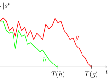
Figure 3: A pair of sample paths (h,g)𝑔(h,g) drawn from ΦπsubscriptΦ𝜋\Phi_{\pi}.

Next, we present the main result of this section, which constructs a monotone coupling distribution of νπ,μπsubscript𝜈𝜋subscript𝜇𝜋\nu_{\pi},\mu_{\pi} by exploiting the differences in node-level transition probabilities.

Theorem 2.

Suppose x,yΩ𝑥𝑦Ωx,y\in\Omega with xΩysubscriptprecedes-or-equalsΩ𝑥𝑦x\preceq_{\Omega}y. For each i𝒩𝑖𝒩i\in\mathcal{N}, define φix,y:{0,1}2[0,1]:superscriptsubscript𝜑𝑖𝑥𝑦superscript01201\varphi_{i}^{x,y}:\{0,1\}^{2}\rightarrow[0,1] according to

xisubscript𝑥𝑖\displaystyle x_{i} =yi=1,{φix,y(0,0)=δ(1p01i(y))φix,y(0,1)=δ(p01i(y)p01,di(x))φix,y(1,0)=0φix,y(1,1)=1δ(1p01,di(x))formulae-sequenceabsentsubscript𝑦𝑖1casessuperscriptsubscript𝜑𝑖𝑥𝑦00absent𝛿1superscriptsubscript𝑝01𝑖𝑦superscriptsubscript𝜑𝑖𝑥𝑦01absent𝛿superscriptsubscript𝑝01𝑖𝑦superscriptsubscript𝑝01𝑑𝑖𝑥superscriptsubscript𝜑𝑖𝑥𝑦10absent0superscriptsubscript𝜑𝑖𝑥𝑦11absent1𝛿1superscriptsubscript𝑝01𝑑𝑖𝑥\displaystyle=y_{i}=1,\ \ \ \begin{cases}\varphi_{i}^{x,y}(0,0)&=\delta(1-p_{01}^{i}(y))\\ \varphi_{i}^{x,y}(0,1)&=\delta(p_{01}^{i}(y)-p_{01,d}^{i}(x))\\ \varphi_{i}^{x,y}(1,0)&=0\\ \varphi_{i}^{x,y}(1,1)&=1-\delta(1-p_{01,d}^{i}(x))\end{cases} (42)
xisubscript𝑥𝑖\displaystyle x_{i} =yi=0,{φix,y(0,0)=1p01i(y)φix,y(0,1)=p01i(y)p01,di(x)φix,y(1,0)=0φix,y(1,1)=p01,di(x)formulae-sequenceabsentsubscript𝑦𝑖0casessuperscriptsubscript𝜑𝑖𝑥𝑦00absent1superscriptsubscript𝑝01𝑖𝑦superscriptsubscript𝜑𝑖𝑥𝑦01absentsuperscriptsubscript𝑝01𝑖𝑦superscriptsubscript𝑝01𝑑𝑖𝑥superscriptsubscript𝜑𝑖𝑥𝑦10absent0superscriptsubscript𝜑𝑖𝑥𝑦11absentsuperscriptsubscript𝑝01𝑑𝑖𝑥\displaystyle=y_{i}=0,\ \ \ \begin{cases}\varphi_{i}^{x,y}(0,0)&=1-p_{01}^{i}(y)\\ \varphi_{i}^{x,y}(0,1)&=p_{01}^{i}(y)-p_{01,d}^{i}(x)\\ \varphi_{i}^{x,y}(1,0)&=0\\ \varphi_{i}^{x,y}(1,1)&=p_{01,d}^{i}(x)\end{cases} (43)
xisubscript𝑥𝑖\displaystyle x_{i} =0,yi=1,{φix,y(0,0)=δ(1p01i(y))φix,y(0,1)=1p01,di(x)δ(1p01i(y))φix,y(1,0)=0φix,y(1,1)=p01,di(x)formulae-sequenceabsent0subscript𝑦𝑖1casessuperscriptsubscript𝜑𝑖𝑥𝑦00absent𝛿1superscriptsubscript𝑝01𝑖𝑦superscriptsubscript𝜑𝑖𝑥𝑦01absent1superscriptsubscript𝑝01𝑑𝑖𝑥𝛿1superscriptsubscript𝑝01𝑖𝑦superscriptsubscript𝜑𝑖𝑥𝑦10absent0superscriptsubscript𝜑𝑖𝑥𝑦11absentsuperscriptsubscript𝑝01𝑑𝑖𝑥\displaystyle=0,y_{i}=1,\begin{cases}\varphi_{i}^{x,y}(0,0)&=\delta(1-p_{01}^{i}(y))\\ \varphi_{i}^{x,y}(0,1)&=1-p_{01,d}^{i}(x)-\delta(1-p_{01}^{i}(y))\\ \varphi_{i}^{x,y}(1,0)&=0\\ \varphi_{i}^{x,y}(1,1)&=p_{01,d}^{i}(x)\end{cases} (44)

Also, define φx,y:Ω2[0,1]:superscript𝜑𝑥𝑦superscriptΩ201\varphi^{x,y}:\Omega^{2}\rightarrow[0,1] for xΩysubscriptprecedes-or-equalsΩ𝑥𝑦x\preceq_{\Omega}y by

φx,y(ω,ω)i=1nφix,y(ωi,ωi)ω,ωΩ.formulae-sequencesuperscript𝜑𝑥𝑦𝜔superscript𝜔superscriptsubscriptproduct𝑖1𝑛subscriptsuperscript𝜑𝑥𝑦𝑖subscript𝜔𝑖superscriptsubscript𝜔𝑖for-all𝜔superscript𝜔Ω\varphi^{x,y}(\omega,\omega^{\prime})\triangleq\prod_{i=1}^{n}\varphi^{x,y}_{i}(\omega_{i},\omega_{i}^{\prime})\ \ \forall\omega,\omega^{\prime}\in\Omega. (45)

Lastly, define Φπ:Γ2[0,1]:subscriptΦ𝜋superscriptΓ201\Phi_{\pi}:\Gamma^{2}\rightarrow[0,1] for any πΔ(Ω)𝜋ΔΩ\pi\in\Delta(\Omega) by

Φπ(h,g)χ(h0=g0)π(h0)t=0T(g)1φht,gt(ht+1,gt+1).subscriptΦ𝜋𝑔𝜒superscript0superscript𝑔0𝜋superscript0superscriptsubscriptproduct𝑡0𝑇𝑔1superscript𝜑superscript𝑡superscript𝑔𝑡superscript𝑡1superscript𝑔𝑡1\Phi_{\pi}(h,g)\triangleq\chi(h^{0}=g^{0})\pi(h^{0})\prod_{t=0}^{T(g)-1}\varphi^{h^{t},g^{t}}(h^{t+1},g^{t+1}). (46)

Then ΦπsubscriptΦ𝜋\Phi_{\pi} is a monotone coupling of νπ,μπsubscript𝜈𝜋subscript𝜇𝜋\nu_{\pi},\mu_{\pi}.

Proof.

See Appendix. ∎

The couplings between node-level transition probabilities φix,ysuperscriptsubscript𝜑𝑖𝑥𝑦\varphi_{i}^{x,y} given in (42)-(44) are used to establish a coupling between benchmark and distancing probability distributions on sample paths in (46). The form of the φix,ysuperscriptsubscript𝜑𝑖𝑥𝑦\varphi_{i}^{x,y} is identical to the method in which two biased coins are coupled in (29). When the coupling rule is applied to each node’s probability of infection, it ensures no node can be infected in the distancing chain while being susceptible in the benchmark chain. Consequently, the monotone coupling ΦπsubscriptΦ𝜋\Phi_{\pi} is a distribution on pairs of sample paths (h,g)𝑔(h,g) satisfying h0=g0superscript0superscript𝑔0h^{0}=g^{0}, hΓgsubscriptprecedes-or-equalsΓ𝑔h\preceq_{\Gamma}g (see Figure 3) and marginally, hνπsimilar-tosubscript𝜈𝜋h\sim\nu_{\pi}, gμπsimilar-to𝑔subscript𝜇𝜋g\sim\mu_{\pi}. The next result characterizes the difference between μπsubscript𝜇𝜋\mu_{\pi} and νπsubscript𝜈𝜋\nu_{\pi}-expectations of any non-negative increasing function on the sample paths ΓΓ\Gamma with respect to the coupling distribution ΦπsubscriptΦ𝜋\Phi_{\pi}.

Corollary 2.

For any increasing +subscript\mathbb{Z}_{+}-valued random variable Z𝑍Z in ΓΓ\Gamma,

𝔼μπ(Z)𝔼νπ(Z)=τ=0Φπ(Zτc,Zτ).subscript𝔼subscript𝜇𝜋𝑍subscript𝔼subscript𝜈𝜋𝑍superscriptsubscript𝜏0subscriptΦ𝜋superscriptsubscript𝑍𝜏𝑐subscript𝑍𝜏\mathbb{E}_{\mu_{\pi}}(Z)-\mathbb{E}_{\nu_{\pi}}(Z)=\sum_{\tau=0}^{\infty}\Phi_{\pi}(Z_{\tau}^{c},Z_{\tau}). (47)

where Zτ={xΓ:Z(x)>τ}subscript𝑍𝜏conditional-set𝑥Γ𝑍𝑥𝜏Z_{\tau}=\{x\in\Gamma:Z(x)>\tau\}.

Proof.

Immediate from Theorem 2 and Proposition 1. ∎

One can think of an increasing Z:Γ+:𝑍ΓsubscriptZ:\Gamma\rightarrow\mathbb{Z}_{+} as an epidemic cost metric. Here, Φπ(Zτc,Zτ)subscriptΦ𝜋superscriptsubscript𝑍𝜏𝑐subscript𝑍𝜏\Phi_{\pi}(Z_{\tau}^{c},Z_{\tau}) is simply the probability a benchmark sample path g𝑔g incurs a cost greater than τ𝜏\tau, while the corresponding distancing sample path hh costs less than τ𝜏\tau, where (h,g)Φπsimilar-to𝑔subscriptΦ𝜋(h,g)\sim\Phi_{\pi}. The difference (47) encodes many complex dependencies on the epidemic parameters δ𝛿\delta and β𝛽\beta, the awareness weight α𝛼\alpha, and the graphs 𝒢Csubscript𝒢𝐶\mathcal{G}_{C} and 𝒢Isubscript𝒢𝐼\mathcal{G}_{I}.

The following result establishes stochastic domination of the distancing chain by the benchmark chain.

Corollary 3.

The benchmark chain stochastically dominates the distancing chain on sample paths, i.e. μπνπsucceeds-or-equalssubscript𝜇𝜋subscript𝜈𝜋\mu_{\pi}\succeq\nu_{\pi}.

Proof.

For any upper set ΓΓ\mathcal{I}\subset\Gamma, χ()subscript𝜒\chi_{\mathcal{I}}(\cdot) is increasing in ΓΓ\Gamma. By (47),

μπ()νπ()subscript𝜇𝜋subscript𝜈𝜋\displaystyle\mu_{\pi}(\mathcal{I})-\nu_{\pi}(\mathcal{I}) =𝔼μπ(χ)𝔼νπ(χ)absentsubscript𝔼subscript𝜇𝜋subscript𝜒subscript𝔼subscript𝜈𝜋subscript𝜒\displaystyle=\mathbb{E}_{\mu_{\pi}}(\chi_{\mathcal{I}})-\mathbb{E}_{\nu_{\pi}}(\chi_{\mathcal{I}})
=Φπ(c,)0absentsubscriptΦ𝜋superscript𝑐0\displaystyle=\Phi_{\pi}(\mathcal{I}^{c},\mathcal{I})\geq 0 (48)

The difference in probability (48) confirms the intuition gained from Corollary 1 that sample paths with consistently high numbers of infected individuals are more probable under the benchmark chain. The closed-form differences (47) and (48) provide a stochastic analogue to Corollary 1, which only establishes inequality between the mean-field metastable states of benchmark and distancing models.

Some examples of increasing +subscript\mathbb{Z}_{+}-valued random variables in ΓΓ\Gamma are

  • The absorption time T:Γ+:𝑇ΓsubscriptT:\Gamma\rightarrow\mathbb{Z}_{+}, defined by (36).

  • The social cost up to time m𝑚m, defined by gt=0m|gt|maps-to𝑔superscriptsubscript𝑡0𝑚superscript𝑔𝑡g\mapsto\sum_{t=0}^{m}|g^{t}|, where |s|i𝒩si𝑠subscript𝑖𝒩subscript𝑠𝑖|s|\triangleq\sum_{i\in\mathcal{N}}s_{i} for sΩ𝑠Ωs\in\Omega.

  • The “epidemic spread”, or how many unique nodes that contract the disease in a given amount of time m𝑚m. This is given by gi𝒩χEi(g)maps-to𝑔subscript𝑖𝒩subscript𝜒subscript𝐸𝑖𝑔g\mapsto\sum_{i\in\mathcal{N}}\chi_{E_{i}}(g), where Ei={g:t=0mgit>0}subscript𝐸𝑖conditional-set𝑔superscriptsubscript𝑡0𝑚superscriptsubscript𝑔𝑖𝑡0E_{i}=\{g:\sum_{t=0}^{m}g_{i}^{t}>0\}. This metric is investigated on different network structures in the next section.
Refer to caption
(a)
Refer to caption
(b)
Refer to caption
(c)
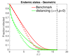
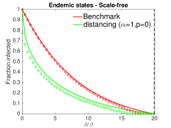
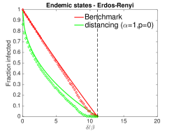
Figure 4: Norms of the nontrivial fixed points (solid lines) and long-run fraction of infected in stochastic simulations (diamonds) in the range of epidemic persistence, δ/β[0,λmax(AC)]𝛿𝛽0subscript𝜆maxsubscript𝐴𝐶\delta/\beta\in[0,\lambda_{\text{max}}(A_{C})], for n=1000𝑛1000n=1000 node networks. The fixed points are computed by iterating the MFA dynamics (14) and (15) with an arbitrary initial condition until convergence. The stochastic long-run infected fractions are computed by averaging the levels of epidemic states in the latter half of a sample run of length 200. Vertical dashed lines indicate λmax(AC)subscript𝜆maxsubscript𝐴𝐶\lambda_{\text{max}}(A_{C}). (a) Erdős-Renyi random network with pER=.01subscript𝑝ER.01p_{\text{ER}}=.01, λmax(AC)=11.1subscript𝜆maxsubscript𝐴𝐶11.1\lambda_{\text{max}}(A_{C})=11.1. Here, pER>logn/nsubscript𝑝ER𝑛𝑛p_{\text{ER}}>\log n/n, the regime where the network is connected with high probability. (b) Geometric random graph with r=.0564𝑟.0564r=.0564, λmax(AC)=16.52subscript𝜆maxsubscript𝐴𝐶16.52\lambda_{\text{max}}(A_{C})=16.52. (c) Scale-free generated from the PA algorithm with m=5𝑚5m=5, λmax(AC)=19.9subscript𝜆maxsubscript𝐴𝐶19.9\lambda_{\text{max}}(A_{C})=19.9. The parameters are chosen such that all networks have the same average degree d10𝑑10d\approx 10.
Refer to caption
(a)
Refer to caption
(b)
Refer to caption
(c)
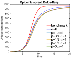
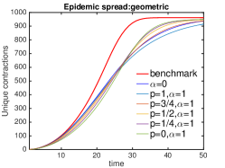
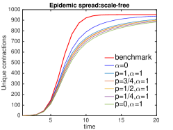
Figure 5: Epidemic spreading as a function of time (same networks as Fig. 4). Local contact information (α𝛼\alpha near 1, p𝑝p near 0) slows spread most effectively for (a),(c), and the early stages of (b), whereas global information (α𝛼\alpha near 0 or α=1,p𝛼1𝑝\alpha=1,p near 1) is least effective. Note the inversion of awareness effectiveness in (b). In these simulations, δ=β=0.2𝛿𝛽0.2\delta=\beta=0.2.

V Simulations on random networks

In this section, we illustrate through numerical simulations how the structure of the contact network 𝒢Csubscript𝒢𝐶\mathcal{G}_{C} affects the course of an epidemic in the presence of awareness and social distancing. Extensive analytical and simulation studies have been conducted without awareness ([1],[2],[3],[5],[33]). Here, we look at three random graph families - geometric, Erdős-Renyi, and scale-free. These networks are relevant in studying epidemic spreading because they exhibit a variety of qualitative features that reflect real-world networks. Geometric networks portray people connected by geographic distance. Erdős-Renyi random networks display a small-world effect common in many real world networks - e.g neural and social influence networks. Online social networks and the World Wide Web are examples of scale-free networks [4].

In our model, the social network 𝒢Isubscript𝒢𝐼\mathcal{G}_{I} is generated directly from 𝒢Csubscript𝒢𝐶\mathcal{G}_{C} via a parameter p(0,1)𝑝01p\in(0,1) through the following procedure: 1) Select a fraction p𝑝p of existing edges in Csubscript𝐶\mathcal{E}_{C} at random and remove them from the edge set; 2) For each of the selected edges, select one of the two end nodes randomly (e.g with probability 1/2) as the root node; 3) For each of the selected root nodes i𝑖i, select ji𝑗𝑖j\neq i uniformly at random and add the edge (i,j)𝑖𝑗(i,j). For p𝑝p close to one, the resulting graph 𝒢I=(𝒩,I)subscript𝒢𝐼𝒩subscript𝐼\mathcal{G}_{I}=(\mathcal{N},\mathcal{E}_{I}) exhibits the small-world effect (small average shortest path length and small clustering) [34]. When p=0𝑝0p=0, 𝒢I=𝒢Csubscript𝒢𝐼subscript𝒢𝐶\mathcal{G}_{I}=\mathcal{G}_{C}.

For the contact networks, geometric random graphs are generated by placing n𝑛n points uniformly at random on the unit torus (unit square with periodic boundary conditions). An edge exists between any two points if they are less than a specified distance r(0,1)𝑟01r\in(0,1) away. Erdős-Renyi random graphs are constructed by forming an edge between any two nodes independently with a fixed probability pER(0,1)subscript𝑝ER01p_{\text{ER}}\in(0,1). Scale-free networks are generated by the preferential attachment algorithm [35]: starting with an initial connected graph of m0msubscript𝑚0𝑚m_{0}\geq m nodes, nm0𝑛subscript𝑚0n-m_{0} additional nodes are added sequentially with each incoming node establishing links to m𝑚m existing nodes in the network. The probability a node receives an incoming link is proportional to its degree. We performed simulation analysis on one network from each random graph family. The networks all have 1000 nodes with an average degree of 10, and hence the same number of edges.

In Figure 4, the normalized non-trivial fixed points are characterized for the three random networks in the interval of epidemic persistence. The norms of these points indicate the size of the endemic states and they slightly overestimate the actual long-run infected fraction observed in stochastic simulations of the Markov chains.

In Figure 5, we quantify the “epidemic spread” by the number of unique nodes that contract an infection as time progresses when one uniformly random node is initially infected. This metric is an example of an increasing random variable over sample paths (Section IV) and is helpful in revealing not only how fast an epidemic initially spreads in the network, but also how far-reaching it is. A key observation is that contact awareness (p=0,α=1formulae-sequence𝑝0𝛼1p=0,\alpha=1) slows epidemic spreading better than any other awareness configuration at the beginning of an epidemic. This is intuitively clear since contact awareness provides nodes with the most vital information if they are in danger of getting infected. As p𝑝p increases, 𝒢Isubscript𝒢𝐼\mathcal{G}_{I} deviates more from 𝒢Csubscript𝒢𝐶\mathcal{G}_{C} and the information nodes receive become less vital.

Erdős-Renyi and scale-free (with m=5𝑚5m=5) networks admit disease spread throughout the entire network in a short amount of time, even with social distancing (Figure 5(a),5(c)). This is attributed to small average shortest path lengths (Ch. 8 & 12, [4]), allowing the epidemic to quickly spread to other parts of the network. Random geometric networks are characterized by high clustering and large diameter. Clustering slows the spread of an epidemic (Figure 5(b)), but also contributes to increasing the final epidemic size [7]. The virus stays localized and spreads slowly. This explains the inversion of awareness parameters in Figure 5(b). By the time the epidemic first reaches its endemic level around t=20𝑡20t=20, many nodes have not yet been exposed because at this point their local communities are untouched. Thus, having global or long-range social awareness (low α𝛼\alpha or high p𝑝p) is more beneficial over contact awareness.

VI Conclusions

We modified the benchmark networked SIS epidemic process to include agent awareness, where prevalence-based information comes from social contacts and a global broadcast of the overall infected fraction. Agents take social distancing actions based on the level of information received, which reduces their probabilities of getting infected. We showed that awareness does not change the epidemic threshold for persistence by proving existence of a nontrivial fixed point in the mean-field approximation. Any nontrivial fixed point of the distancing model is strictly component-wise less than the unique nontrivial fixed point of the benchmark model.

We provided a full stochastic comparison analysis between the benchmark and distancing chains in terms of their respective probability distributions on sample paths by constructing a monotone coupling. The construction relies on exploiting the differences in node transition probabilities between the two chains. Consequently, adding awareness reduces the expectation of any increasing random variable on sample paths and we obtain a closed form expression for the reduction. This implies the benchmark distribution on sample paths stochastically dominates the distancing distribution.

In simulations, we showed epidemic spreading heavily depends on the network structure. In particular, qualitative features such as small-world effects, clustering, and diameter explain the results seen in simulations. We also concluded local contact awareness is the most effective at slowing epidemic spread, and global awareness is the least effective.

Proof of Theorem 2.

When xΩysubscriptprecedes-or-equalsΩ𝑥𝑦x\preceq_{\Omega}y, the φix,ysubscriptsuperscript𝜑𝑥𝑦𝑖\varphi^{x,y}_{i} are well-defined probabilities since p01i(y)p01,di(x)0superscriptsubscript𝑝01𝑖𝑦superscriptsubscript𝑝01𝑑𝑖𝑥0p_{01}^{i}(y)-p_{01,d}^{i}(x)\geq 0 and 1p01,di(x)δ(1p01i(y))>01superscriptsubscript𝑝01𝑑𝑖𝑥𝛿1superscriptsubscript𝑝01𝑖𝑦01-p_{01,d}^{i}(x)-\delta(1-p_{01}^{i}(y))>0. One can see by inspection that φix,ysubscriptsuperscript𝜑𝑥𝑦𝑖\varphi^{x,y}_{i} is a monotone coupling of id(x,)superscriptsubscript𝑖𝑑𝑥\mathbb{P}_{i}^{d}(x,\cdot) and i(y,)subscript𝑖𝑦\mathbb{P}_{i}(y,\cdot) defined in (9), (10) and (3), (4) respectively.

Observe from (45), φx,y(ω,ω)>0superscript𝜑𝑥𝑦𝜔superscript𝜔0\varphi^{x,y}(\omega,\omega^{\prime})>0 implies xΩysubscriptprecedes-or-equalsΩ𝑥𝑦x\preceq_{\Omega}y and ωΩωsubscriptprecedes-or-equalsΩ𝜔superscript𝜔\omega\preceq_{\Omega}\omega^{\prime}. Consequently, φx,ysuperscript𝜑𝑥𝑦\varphi^{x,y} is a monotone coupling of Kd(x,),K(y,)subscript𝐾𝑑𝑥𝐾𝑦K_{d}(x,\cdot),K(y,\cdot):

ωΩωφx,y(ω,ω)subscriptsubscriptsucceeds-or-equalsΩsuperscript𝜔𝜔superscript𝜑𝑥𝑦𝜔superscript𝜔\displaystyle\sum_{\omega^{\prime}\succeq_{\Omega}\omega}\varphi^{x,y}(\omega,\omega^{\prime}) =i=1n(ωiωiφix,y(ωi,ωi))absentsuperscriptsubscriptproduct𝑖1𝑛subscriptsubscriptsuperscript𝜔𝑖subscript𝜔𝑖subscriptsuperscript𝜑𝑥𝑦𝑖subscript𝜔𝑖subscriptsuperscript𝜔𝑖\displaystyle=\prod_{i=1}^{n}\left(\sum_{\omega^{\prime}_{i}\geq\omega_{i}}\varphi^{x,y}_{i}(\omega_{i},\omega^{\prime}_{i})\right) (49)
=i=1nid(x,ωi)absentsuperscriptsubscriptproduct𝑖1𝑛superscriptsubscript𝑖𝑑𝑥subscript𝜔𝑖\displaystyle=\prod_{i=1}^{n}\mathbb{P}_{i}^{d}(x,\omega_{i}) (50)
=Kd(x,ω)absentsubscript𝐾𝑑𝑥𝜔\displaystyle=K_{d}(x,\omega) (51)

By a completely analogous computation, we obtain ωΩωφx,y(ω,ω)=K(y,ω)subscriptsubscriptprecedes-or-equalsΩsuperscript𝜔𝜔superscript𝜑𝑥𝑦superscript𝜔𝜔𝐾𝑦𝜔\sum_{\omega^{\prime}\preceq_{\Omega}\omega}\varphi^{x,y}(\omega^{\prime},\omega)=K(y,\omega).

Also, notice from (46) that Φπ(h,g)>0subscriptΦ𝜋𝑔0\Phi_{\pi}(h,g)>0 implies h0=g0superscript0superscript𝑔0h^{0}=g^{0} and hΓgsubscriptprecedes-or-equalsΓ𝑔h\preceq_{\Gamma}g. Consequently, ΦπsubscriptΦ𝜋\Phi_{\pi} is a monotone coupling of νπ,μπsubscript𝜈𝜋subscript𝜇𝜋\nu_{\pi},\mu_{\pi}:

gΓhΦπ(h,g)subscriptsubscriptsucceeds-or-equalsΓ𝑔subscriptΦ𝜋𝑔\displaystyle\sum_{g\succeq_{\Gamma}h}\Phi_{\pi}(h,g) =gΓhg0=h0π(h0)t=0T(g)1φht,gt(ht+1,gt+1)absentsubscriptsubscriptsucceeds-or-equalsΓ𝑔superscript𝑔0superscript0𝜋superscript0superscriptsubscriptproduct𝑡0𝑇𝑔1superscript𝜑superscript𝑡superscript𝑔𝑡superscript𝑡1superscript𝑔𝑡1\displaystyle=\sum_{\begin{subarray}{c}g\succeq_{\Gamma}h\\ g^{0}=h^{0}\end{subarray}}\pi(h^{0})\prod_{t=0}^{T(g)-1}\varphi^{h^{t},g^{t}}(h^{t+1},g^{t+1}) (52)
=π(h0)t=1T(h)gtΩhtφht1,gt1(ht,gt)absent𝜋superscript0superscriptsubscriptproduct𝑡1𝑇subscriptsubscriptsucceeds-or-equalsΩsuperscript𝑔𝑡superscript𝑡superscript𝜑superscript𝑡1superscript𝑔𝑡1superscript𝑡superscript𝑔𝑡\displaystyle=\pi(h^{0})\prod_{t=1}^{T(h)}\sum_{g^{t}\succeq_{\Omega}h^{t}}\varphi^{h^{t-1},g^{t-1}}(h^{t},g^{t}) (53)
=π(h0)t=1T(h)Kd(ht1,ht)absent𝜋superscript0superscriptsubscriptproduct𝑡1𝑇subscript𝐾𝑑superscript𝑡1superscript𝑡\displaystyle=\pi(h^{0})\prod_{t=1}^{T(h)}K_{d}(h^{t-1},h^{t}) (54)
=νπ(h)absentsubscript𝜈𝜋\displaystyle=\nu_{\pi}(h) (55)

The equality (53) is the combinatorial form of writing (52), and the product terminates at T(h)𝑇T(h) because 1) gΓhsubscriptsucceeds-or-equalsΓ𝑔g\succeq_{\Gamma}h implies T(g)T(h)𝑇𝑔𝑇T(g)\geq T(h), 2) ht=𝕠superscript𝑡𝕠h^{t}=\mathbb{o} for all tT(h)𝑡𝑇t\geq T(h) and 3) for any t>T(h)𝑡𝑇t>T(h),

gtΩhtφht1,gt1(ht,gt)subscriptsubscriptsucceeds-or-equalsΩsuperscript𝑔𝑡superscript𝑡superscript𝜑superscript𝑡1superscript𝑔𝑡1superscript𝑡superscript𝑔𝑡\displaystyle\sum_{g^{t}\succeq_{\Omega}h^{t}}\varphi^{h^{t-1},g^{t-1}}(h^{t},g^{t}) =gtΩφ𝕠,gt1(𝕠,gt)=Kd(𝕠,𝕠)absentsubscriptsuperscript𝑔𝑡Ωsuperscript𝜑𝕠superscript𝑔𝑡1𝕠superscript𝑔𝑡subscript𝐾𝑑𝕠𝕠\displaystyle=\sum_{g^{t}\in\Omega}\varphi^{\mathbb{o},g^{t-1}}(\mathbb{o},g^{t})=K_{d}(\mathbb{o},\mathbb{o})
=1absent1\displaystyle=1

By an analogous computation, hΓgΦπ(h,g)=μπ(g)subscriptsubscriptprecedes-or-equalsΓ𝑔subscriptΦ𝜋𝑔subscript𝜇𝜋𝑔\sum_{h\preceq_{\Gamma}g}\Phi_{\pi}(h,g)=\mu_{\pi}(g). ∎

Acknowledgements

This work is supported by ARO grant #W911NF-14-1-0402, and supported in part by KAUST. The authors thank J. Walker Gussler (Georgia Inst. Tech.) for his contribution in the simulations.

References

  • [1] Y. Wang, D. Chakrabarti, C. Wang, and C. Faloutsos, “Epidemic spreading in real networks: an eigenvalue viewpoint,” in Reliable Distributed Systems, 2003. Proceedings. 22nd International Symposium on, Oct 2003, pp. 25–34.
  • [2] A. Ganesh, L. Massoulie, and D. Towsley, “The effect of network topology on the spread of epidemics,” in INFOCOM 2005. 24th Annual Joint Conference of the IEEE Computer and Communications Societies. Proceedings IEEE, vol. 2, March 2005, pp. 1455–1466 vol. 2.
  • [3] V. M. Eguíluz and K. Klemm, “Epidemic threshold in structured scale-free networks,” Phys. Rev. Lett., vol. 89, p. 108701, Aug 2002.
  • [4] M. Newman, Networks: An Introduction.   New York, NY, USA: Oxford University Press, Inc., 2010.
  • [5] P. Van Mieghem, J. Omic, and R. Kooij, “Virus spread in networks,” Networking, IEEE/ACM Transactions on, vol. 17, no. 1, pp. 1–14, Feb 2009.
  • [6] H. J. Ahn and B. Hassibi, “Global dynamics of epidemic spread over complex networks,” in Decision and Control (CDC), 2013 IEEE 52nd Annual Conference on, Dec 2013, pp. 4579–4585.
  • [7] E. M. Volz, J. C. Miller, A. Galvani, and L. Ancel Meyers, “Effects of heterogeneous and clustered contact patterns on infectious disease dynamics,” PLoS Comput Biol, vol. 7, no. 6, p. e1002042, 06 2011.
  • [8] E. Bodine-Baron, S. Bose, B. Hassibi, and A. Wierman, “Minimizing the social cost of an epidemic,” in Game Theory for Networks, ser. Lecture Notes of the Institute for Computer Sciences, Social Informatics and Telecommunications Engineering, R. Jain and R. Kannan, Eds.   Springer Berlin Heidelberg, 2012, vol. 75, pp. 594–607.
  • [9] K. Drakopoulos, A. Ozdaglar, and J. Tsitsiklis, “An efficient curing policy for epidemics on graphs,” in Decision and Control (CDC), 2014 IEEE 53rd Annual Conference on, Dec 2014, pp. 4447–4454.
  • [10] V. Preciado, M. Zargham, C. Enyioha, A. Jadbabaie, and G. Pappas, “Optimal resource allocation for network protection against spreading processes,” Control of Network Systems, IEEE Transactions on, vol. 1, no. 1, pp. 99–108, March 2014.
  • [11] J. Omic, A. Orda, and P. Van Mieghem, “Protecting against network infections: A game theoretic perspective,” in INFOCOM 2009, IEEE, April 2009, pp. 1485–1493.
  • [12] S. Trajanovski, Y. Hayel, E. Altman, H. Wang, and P. Van Mieghem, “Decentralized protection strategies against sis epidemics in networks,” Control of Network Systems, IEEE Transactions on, vol. 2, no. 4, pp. 406–419, Dec 2015.
  • [13] M. L. Ndeffo Mbah, J. Liu, C. T. Bauch, Y. I. Tekel, J. Medlock, L. A. Meyers, and A. P. Galvani, “The impact of imitation on vaccination behavior in social contact networks,” PLoS Comput Biol, vol. 8, no. 4, p. e1002469, 04 2012.
  • [14] C. Molina and D. J. D. Earn, “Game theory of pre-emptive vaccination before bioterrorism or accidental release of smallpox,” Journal of The Royal Society Interface, vol. 12, no. 107, 2015.
  • [15] C. T. Bauch and D. J. D. Earn, “Vaccination and the theory of games,” Proceedings of the National Academy of Sciences of the United States of America, vol. 101, no. 36, pp. 13 391–13 394, 2004.
  • [16] G. K. SteelFisher, R. J. Blendon, M. M. Bekheit, and K. Lubell, “The public’s response to the 2009 h1n1 influenza pandemic,” New England Journal of Medicine, vol. 362, no. 22, p. e65, 2010, pMID: 20484390.
  • [17] A. Pandey, K. E. Atkins, J. Medlock, N. Wenzel, J. P. Townsend, J. E. Childs, T. G. Nyenswah, M. L. Ndeffo-Mbah, and A. P. Galvani, “Strategies for containing ebola in west africa,” Science, vol. 346, no. 6212, pp. 991–995, 2014.
  • [18] C. T. Bauch and A. P. Galvani, “Social factors in epidemiology,” Science, vol. 342, no. 6154, pp. 47–49, 2013.
  • [19] Z. Wang, M. A. Andrews, Z.-X. Wu, L. Wang, and C. T. Bauch, “Coupled disease–behavior dynamics on complex networks: A review,” Physics of Life Reviews, vol. 15, pp. 1 – 29, 2015.
  • [20] S. Funk, E. Gilad, C. Watkins, and V. A. A. Jansen, “The spread of awareness and its impact on epidemic outbreaks,” Proceedings of The National Academy of Sciences, vol. 106, pp. 6872–6877, 2009.
  • [21] T. C. Reluga, “Game theory of social distancing in response to an epidemic,” PLoS Comput Biol, vol. 6, no. 5, p. e1000793, 05 2010.
  • [22] N. Perra, D. Balcan, B. Gonçalves, and A. Vespignani, “Towards a characterization of behavior-disease models,” PLoS ONE, vol. 6, 08 2011.
  • [23] C. Granell, S. Gómez, and A. Arenas, “Dynamical interplay between awareness and epidemic spreading in multiplex networks,” Phys. Rev. Lett., vol. 111, p. 128701, Sep 2013. [Online]. Available: http://link.aps.org/doi/10.1103/PhysRevLett.111.128701
  • [24] ——, “Competing spreading processes on multiplex networks: Awareness and epidemics,” Phys. Rev. E, vol. 90, p. 012808, Jul 2014. [Online]. Available: http://link.aps.org/doi/10.1103/PhysRevE.90.012808
  • [25] M. Ogura and V. M. Preciado, “Cost-optimal switching protection strategy in adaptive networks,” in 2015 54th IEEE Conference on Decision and Control (CDC), Dec 2015, pp. 3574–3579.
  • [26] H.-F. Zhang, J.-R. Xie, M. Tang, and Y.-C. Lai, “Suppression of epidemic spreading in complex networks by local information based behavioral responses,” Chaos, vol. 24, no. 4, 2014.
  • [27] Q. Wu, X. Fu, M. Small, and X.-J. Xu, “The impact of awareness on epidemic spreading in networks,” Chaos, vol. 22, no. 1, 2012.
  • [28] K. Paarporn, C. Eksin, J. S. Weitz, and J. S. Shamma, “Epidemic spread over networks with agent awareness and social distancing,” in 2015 53rd Annual Allerton Conference on Communication, Control, and Computing (Allerton), Sept 2015, pp. 51–57.
  • [29] ——, “The effect of awareness on networked sis epidemics,” in Decision and Control (CDC), 2016 IEEE 55th Annual Conference on (submitted), Dec 2016.
  • [30] H. J. Ahn and B. Hassibi, “On the mixing time of the sis markov chain model for epidemic spread,” in Decision and Control (CDC), 2014 IEEE 53rd Annual Conference on, Dec 2014, pp. 6221–6227.
  • [31] V. I. Istratescu, Fixed Point Theory, An Introduction.   Holland: D.Reidel, 1981.
  • [32] T. Lindvall, Lectures on the Coupling Method, ser. Dover Books on Mathematics Series.   Dover Publications, Incorporated, 2002.
  • [33] R. Pastor-Satorras and A. Vespignani, “Epidemic spreading in scale-free networks,” Phys. Rev. Lett., vol. 86, pp. 3200–3203, Apr 2001.
  • [34] D. J. Watts and S. H. Strogatz, “Collective dynamics of’small-world’networks.” Nature, vol. 393, no. 6684, pp. 409–10, 1998.
  • [35] A.-L. Barabási and R. Albert, “Emergence of scaling in random networks,” Science, vol. 286, no. 5439, pp. 509–512, 1999.